Physical structure of the envelopes of intermediate-mass protostars

Abstract

Context. Intermediate mass protostars provide a bridge between low- and high-mass protostars. Furthermore, they are an important component of the UV interstellar radiation field. Despite their relevance, little is known about their formation process.

Aims. We present a systematic study of the physical structure of five intermediate mass, candidate Class 0 protostars. Our two goals are to shed light on the first phase of intermediate mass star formation and to compare these protostars with low- and high-mass sources.

Methods. We derived the dust and gas temperature and density profiles of the sample. We analysed all existing continuum data on each source and modelled the resulting SED with the 1D radiative transfer code DUSTY. The gas temperature was then predicted by means of a modified version of the code CHT96.

Results. We found that the density profiles of five out of six studied intermediate mass envelopes are consistent with the predictions of the “inside-out” collapse theory. We compared several physical parameters, like the power law index of the density profile, the size, the mass, the average density, the density at 1000 AU and the density at 10 K of the envelopes of low-, intermediate, and high-mass protostars. When considering these various physical parameters, the transition between the three groups appears smooth, suggesting that the formation processes and triggers do not substantially differ.

1 Introduction

Stars are usually catalogued in three groups according to their mass: low-mass ($\mathrel{\hbox{\hbox to0.0pt{\hbox{\lower 4.0pt\hbox{$\sim$}}\hss}\hbox{$<$}}}$2 M_⊙), intermediate mass (IM) and high-mass ($\mathrel{\hbox{\hbox to0.0pt{\hbox{\lower 4.0pt\hbox{$\sim$}}\hss}\hbox{$>$}}}$8 M_⊙). The high-mass stars are usually found to form in tight clusters (e.g. Hillenbrand & Hartmann 1998), including many low-mass stars as well. Low-mass stars on their own can be formed in isolation or in loose groups of a few objects per cubic parsec (Gomez et al. 1993). While there is reasonable consensus on the overall process leading to the formation of isolated, low-mass stars (see e.g. Shu & Adams 1987), the situation for high-mass star formation is much more confusing. The major problem is that a central object with M $\mathrel{\hbox{\hbox to0.0pt{\hbox{\lower 4.0pt\hbox{$\sim$}}\hss}\hbox{$>$}}}$ 8 M_⊙ produces a radiative pressure stronger than the gravitational pressure, which should stop the accretion. Therefore stars with a mass greater than $\sim$8 M_⊙ cannot be formed in a simple-minded fully gravitationally driven process and other mechanisms need to be considered. Studying the differences in observed environments, several authors have proposed that high-mass stars are formed by the coalescence of lower-mass stars, while other authors favor “monolithic” formation (see for example the recent review by Beuther et al. 2007), where turbulence or winds/outflows can play a major role (McKee & Tan 2003; Krumholz et al. 2005).

The differences between low- and high-mass protostars are not only restricted to the dynamics of the formation mechanism. Notable differences also exist when it comes to the chemistry. Bottinelli (2006) compared the abundances of O-bearing complex organic molecules (COMs) present in Hot Cores surrounding high-mass protostars and in Hot Corinos around low-mass protostars. They concluded that the abundances of the O-bearing COMs, compared to methanol or formaldehyde, are about one order of magnitude higher in Hot Corinos than Hot Cores. In addition, significant differences in the abundances of molecules constituting the grain mantles (H₂O, CO, CO₂,CH₃OH, OCN^-) were observed between low- and high-mass protostars (Boogert et al. 2004). Finally, in contrast to high-mass star forming regions, low-mass protostars present an extremely enhanced molecular deuteration, the so-called Super-Deuteration (e.g. Ceccarelli et al. 2007), not observed in high-mass star forming regions.

The IM stars, namely stars whose mass lies in the 2 to 8 M_⊙ range, are crucial in studies of star formation because they provide the link between low- and high-mass stars (Di Francesco et al. 1997; Mannings & Sargent 1997, 2000) and therefore can help to determine whether different formation processes are required. IM stars are also found in clusters (e.g. Testi & Sargent 1998; Neri et al. 2007; Fuente et al. 2007), with a smooth transition towards the low-mass star, loose cluster regime for star masses around 3.5 M_⊙ (Testi et al. 1999). These authors also conclude that IM stars mark the transition from the low-density aggregates of $\mathrel{\hbox{\hbox to0.0pt{\hbox{\lower 4.0pt\hbox{$\sim$}}\hss}\hbox{$<$}}}$ 10 stars per cubic parsec of T Tauri stars to the dense clusters of $\gtrsim$ 10³ stars per cubic parsec associated with massive stars. Finally, IM stars are among the most dominant sources for the interstellar FUV field (e.g. Habing 1968; Gondhalekar & Wilson 1975), which regulates the phases of the ISM in the Galaxy and, in turn, the overall Galaxy star formation process and history. In this context, the study of the formation of the IM stars is not only interesting in itself, but it can also greatly help the debate on the formation of high-mass stars. Indeed, due to their intermediate position, the study of IM protostars provides crucial information about the transition between the two formation regimes, as well as on the limits of the low-mass and high-mass formation scenarios.

Despite their importance, very little is known about the formation and first evolutionary stages of IM stars. Although some individual IM protostars have been studied in detail (Fuente et al. 2007; Neri et al. 2007; Hogerheijde et al. 1999; Schreyer et al. 2002), the situation is so bad that to date we neither have a satisfying sample of Class 0 IM objects, namely objects representing the first phases of stellar formation where the protostar is embedded in its envelope and its luminosity is dominated by the accretion luminosity, nor a systematic study of their physical structure, as in the case for low-mass and high-mass protostars. On the contrary, several previous studies have considered samples of low- and high-mass protostars. Relevant similar studies to the present IM one are those reported by Jørgensen et al. (2002) and Shirley et al. (2002), who targeted 7 and 11 low-mass Class 0 protostars respectively, and the systematic studies by Mueller et al. (2002), Hatchell & van der Tak (2003), Williams et al. (2005) and Van der Tak et al. (2000), who targeted 31, 10, 32, and 9 high-mass protostars respectively. These authors derived the physical structure of the envelope for each protostar using continuum observations coupled with a radiative transfer code assuming a 1D spherical model. Combined, these studies cover a luminosity range of 1 $<$ L${}_{\odot}<$ 22, and 1$\times$10³ $<$ L${}_{\odot}<$ 2$\times$10⁶ for low- and high-mass protostars respectively, leaving a significant gap in luminosity and knowledge.

This paper aims to fill this gap, providing a systematic study of the physical structure of the envelopes of a sample of five IM protostars. In addition, this study will provide a valuable input for future work on the chemical structure of IM protostars (e.g. Alonso-Albi et al. 2009, in prep). The present work follows the method presented in Crimier et al. (2009a) to study the IM protostars OMC2-FIR4. Namely, the combination of sub-millimeter to infrared observations with radiative transfer codes are used to derive the physical structure of each envelope. We selected a sample of five representative candidate Class 0 IM protostars: CB3-mm, Cep E-mm, IC1396 N BIMA 2, NGC7129 FIRS 2, and Serpens FIRS 1. These sources were selected using the following criteria:

• the luminosity is in the 30 to 1000 L_⊙ range (corresponding to a $\sim$ 3 to 9 M_⊙ of ZAMS stars);

• the continuum maps at submillimetre and/or millimetre wavelengths are available;

• the source is closer than 2.5 kpc to the Sun and isolated, namely no source of similar brightness in the submillimetre within an angular distance of $\sim$100^′′.

The coordinates, the distances and the bolometric luminosities of the selected sources are listed in Table 1.

Source	CB3	Cep E	IC1396 N	NGC7129	Serpens
	mm	mm	BIMA 2	FIRS 2	FIRS 1
RA (2000)	00:28:42.1	23:03:12.7	21:40:41.8	21:43:01.5	18:29:49.8
Dec (2000)	56:41:59.4	61:42:27.4	58:16:13.5	66:03:25.0	01:15:18.4
Distance (pc)	2500	730	750	1250	230
Luminosity (L⊙)	1000	100	150	500	33

Table 1: The coordinates, the distances and the bolometric luminosities of the sources of the sample.

This article is organised as follows. Section 2 describes the observations used and the method and tools employed to derive the dust and gas density and temperature profiles. Section 3 first summarises the general results obtained toward the IM protostar sample. Next, for each source, background information, data available, and the results obtained are presented. In Sect. 4, the physical structure of the envelopes of IM protostars obtained in this study are compared with those obtained in previous studies of low- and high-mass protostar envelopes. In this section we also discuss the limitations of our modeling method. Finally, Sect. 5 concludes the article.

2 General method

In this section we present the general method used to derive the dust density and temperature profiles by modelling the continuum maps of each region, plus the Spectral Energy Distribution (SED) from the millimetre to the Mid-Infrared (MIR). We first describe the observations used in the analysis and how the brightness profiles and the SED are derived (Sect. 2.1), and then we present the modelling (Sect. 2.2).

2.1 Continuum emission : observational data

In our analysis we used the maps of the continuum emission at 850 and 450 $\mu$m obtained at the 15 m James Clerk Maxwell Telescope (JCMT). In addition, we took into account the SED of each source from 24 $\mu$m to 1300 $\mu$m data obtained with the Spitzer, IRAS, JCMT and IRAM telescopes. Note that specific details (datasets, pipeline, uncertainties, contamination … etc) are given separately for each source in Sect. 3.

a) Continuum brightness profiles
For each source we retrieved from the JCMT Science Archive the 450 $\mu$m and 850 $\mu$m maps obtained by the focal-plane instrument SCUBA (Submillimetre Common-User Bolometer Array). The data were reduced with the JCMT pipelines SURF V1.6-13, and KAPPA 1.9-7. When multiple observations were available in the archive, we used the most sensitive ones. The angular resolution of the maps is approximately 7.5″and 14.8″at 450 and 850 $\mu$m respectively (see Sect. 2.2 for more details). Based on the many previous JCMT published observations, the calibration uncertainty and noise levels are $\mathrel{\hbox{\hbox to0.0pt{\hbox{\lower 4.0pt\hbox{$\sim$}}\hss}\hbox{$<$}}}$ 10% and 0.04 Jy beam^-1 at 850 $\mu$m and $\mathrel{\hbox{\hbox to0.0pt{\hbox{\lower 4.0pt\hbox{$\sim$}}\hss}\hbox{$<$}}}$ 30% and 0.3 Jy beam^-1 at 450 $\mu$m, respectively. To evaluate the continuum brightness profile (the brightness as a function of the distance from the envelope centre), we averaged the observed flux over annuli with the same distance from the centre of the source. The final uncertainties were evaluated taking into account the calibration uncertainty, the noise levels of the used maps, and the non-sphericity of the source. The non-sphericity of the source is taken into account via the computation of the standard deviation relative to the azimuthal average for each averaged flux of the brightness profile.

b) SED
The SED points at 850 $\mu$m and 450 $\mu$m were obtained integrating the continuum flux profiles previously derived over the full envelope. We also considered the integrated flux at 24 $\mu$m and 70 $\mu$m extracted from the Spitzer Space Telescope Multiband Imaging Photometer (MIPS) maps. To this end, we retrieved the observations from the Spitzer Science archive. The data reduction was performed using the pipeline S16.1.0. The evaluation of the fluxes was done with the same method employed for the maps at 850 $\mu$m and 450 $\mu$m, namely deriving the brightness profiles from the maps and integrating over each annuli. We evaluated the uncertainties according to the instrument uncertainties and varying the outer radius of the envelope to account for the uncertainty in the envelope size. To do this we first set the outer radius equal to where the flux profile becomes flat (because dominated by the noise or the flux of the parent cloud) and varied this value up to 100 $\%$. In general, the uncertainties remain relatively constant for variations larger than 30-50$\%$. Note that we checked a posteriori that our adopted radius and variation range is constitent with the outer radius obtained after the modelling. Finally, we also considered the IRAS fluxes at 60 $\mu$m and 100 $\mu$m, respectively, taken from the literature or the IRAS Point Source Catalog v2.0. The SED fluxes of each source and their uncertainties are reported in Table 2.

Source	CB3	Cep E	IC1396 N	NGC7129	Serpens
	mm	mm	BIMA 2	FIRS 2	FIRS 1
F24μm (Jy) - Spitzer	$1.4\pm 0.8$	$6.0\pm 3.0$	$2.3\pm 2.0$	$6.0\pm 3.0$	$3.0\pm 1.0$
F60μm (Jy) - IRAS	$31\pm 15$	$61\pm 30$	-	-	-
F70μm (Jy) - Spitzer	$58\pm 20$	$100\pm 40$	-	$110\pm 60$	$135\pm 50$
F100μm (Jy) - IRAS	$110\pm 55$	$110\pm 55$	-	-	-
F450μm (Jy) - JCMT	$30\pm 10$	$44\pm 10$	$100\pm 30$	$80\pm 40$	$130\pm 40$
F850μm (Jy) - JCMT	$2.0\pm 1.0$	$4.1\pm 1.3$	$17\pm 7.0$	$4.8\pm 2.0$	$14\pm 4.0$
F1300μm (Jy) - IRAM30m	-	$1.0\pm 0.2$	-	$2.2\pm 0.5$	-

Table 2: Continuum fluxes integrated over the envelope of each source and used in the SED analysis.

2.2 Continuum emission : modelling

To derive the dust temperature and density profiles of the envelope, we used the 1D radiative transfer code DUSTY (Ivezic & Elitzur 1997). Briefly, giving as input the temperature and size of the central object and a dust density profile, DUSTY self-consistently computes the dust temperature profile and the dust emission. The comparison between the computed 450 $\mu$m, 850 $\mu$m and 1300 $\mu$m brightness profiles (namely the brightness versus the distance from the centre of the envelope) and integrated SED against the observed brightness profiles and integrated SED (see previous paragraph) allows one to constrain the density profile and, consequently, the temperature profile of the envelope.

To be compared against the observations, the theoretical emission must be convolved with the beam pattern of each telescope. Following the recommendations for the JCMT, the beam is assumed to be a combination of three Gaussian curves: at 850 $\mu$m we used HPBWs of 14.5″, 60″, and 120″, with amplitudes of 0.976, 0.022, and 0.002 respectively; at 450 $\mu$m the HPBWs are 8″, 30″, and 120″. with amplitude ratios of 0.934, 0.06, and 0.006, respectively (Sandell & Weintraub 2001).

In all sources we assumed that the envelope density follows a single index power law

$$n(r)=n_{0}\times\left(\frac{r_{0}}{r}\right)^{\alpha},$$ (1)

where the power law index, $\alpha$, and the density, $n_{0}$, at $r_{0}$ are free parameters of the model. The envelope is assumed to start at a radius r_in and extends to r_out. Both r_in and r_out are additional free parameters of the model. The last input into DUSTY is the temperature of the central source, T_∗, here assumed to be 5000 K. We verified that the choice of this last parameter does not influence the results. Indeed, given the high optical thickness of the envelopes at the wavelengths where the central source emits, the model outputs are not sensitive to the T_∗ value. Finally, the opacity of the dust as function of the wavelength is another parameter of DUSTY. Following numerous previous studies (van der Tak et al. 1999; Evans et al. 2001; Shirley et al. 2002; Young et al. 2003), we adopted the dust opacity calculated by Ossenkopf & Henning (1994), specifically their OH5 dust model, which refers to grains coated by ice. We also obtained a lower limit to T_in (the temperature at R_in) of 300 K: any higher value for T_in would give similar results. Again, given the high optical thickness of the envelope at short wavelengths and the low contribution from the dust at T $>$ 300 K to the sub-millimetre emission ( as the NIR emission is mainly from the very inner part, i.e. a small volume), increasing T_in does not make a difference to the resulting best-fit.

In summary, the output of DUSTY depends on four free parameters: $\alpha$, $n_{0}$, r_in and r_out. In practice, the DUSTY input parameters are the power law index, $\alpha$, the optical thickness at 100 $\mu$m, $\tau_{100}$, the ratio between the inner and outer radius, Y (=r_out/r_in) and the temperature at the inner radius T_in. The optical thickness is, in turn, proportional to the dust column density which depends on $n_{0}$ and the physical thickness of the envelope. Note that because the beam sizes of the available maps are relatively large ($\geq 7.5$″, which corresponds to a radius of $\geq 3250$ AU for a source at a distance of 1000 pc), the inner regions of the envelopes are relatively unconstrained by the available observational data. Finally, as explained in Ivezic & Elitzur (1997), DUSTY gives scaleless results (which make it very powerful because the same grid of models can be applied to many different sources). To compare the DUSTY output with actual observations it is necessary to scale the output by the source bolometric luminosity, L_bol, and the distance to the source. Note that the bolometric luminosity is estimated by integrating the emission across the full spectrum. By definition, this can only be done when the entire SED is known. This is exactly one of the outputs of the modelling. Therefore, we re-evaluate the luminosity of each source iteratively from the best-fit model, by minimising the $\chi^{2}$.

We ran a grid of models to cover the parameter space as reported in Table 3.

Parameter	Range	step
$\alpha$	0.2-2.5	0.1
Y	50-2000	10
$\tau_{100}$	0.1-10.	0.1
Tin	300 K
T∗	5000 K

Table 3: Range of the input parameters to DUSTY covered in the present study. The range of the $\alpha$, Y and $\tau_{100}$ parameters are covered by increasing by a constant value at each step of the grid reported in the third column. Note that T_in and T${}_{{}_{*}}$ remain fixed as they do not influence the results (see text).

The best-fit model is found by minimising the $\chi^{2}$ with an iterated two-steps procedure. First, we used the observed brightness profiles at 450 $\mu m$ and 850 $\mu m$ to constrain $\alpha$ and Y, assuming a value for $\tau_{100}$. The $\chi^{2}_{red}$ computed during this first step are reported as $\chi^{2}_{red}$-maps in Table 4. Second, we constrain the optical thickness $\tau_{100}$ by comparing the computed and observed SED, assuming the $\alpha$ and Y of the previous step. The new $\tau_{100}$ is used for the next iteration and the process is repeared. The $\chi^{2}_{red}$ computed during this second step are reported as $\chi^{2}_{red}$-SED in Table 4. In practice, the iteration converges in two steps. This occurs because the normalised brightness profiles are only very weakly dependent on $\tau_{100}$, while they are very dependent on the sizes of the envelope and on the slope of the density profile (see also Jørgensen et al. 2002; Schöier et al. 2002; Crimier et al. 2009a). On the contrary, the optical thickness depends mostly on the absolute column density of the envelope, which is constrained by the SED.

2.3 Gas temperature profile : model description

Ceccarelli et al. (1996), Crimier et al. (2009a) and Doty & Neufeld (1997) showed that the gas can be thermally decoupled from the dust in the inner regions of low-, intermediate and high-mass protostellar envelopes. The decoupling occurs mainly in the inner part of the envelopes: for example whereas T${}_{dust}\sim$ 150 K at 200 AU, T${}_{gas}\sim$ 90 K. Note that in the outer envelope, where T${}_{dust}\mathrel{\hbox{\hbox to0.0pt{\hbox{\lower 4.0pt\hbox{$\sim$}}\hss}\hbox{$<$}}}$ 100K, gas and dust temperature only differ by a few percents (see discussion in Crimier et al. 2009a). The reason for this decoupling is the high water abundance in the gas phase caused by the sublimation of grain mantles. We therefore explicitly computed the gas temperature profile of the envelope surrounding each source by finding the equilibrium temperature obtained by equating the gas cooling and heating terms at each radius. Following the method described by Ceccarelli et al. (1996), we considered heating from the gas compression (due to the collapse), dust-gas collisions, photo-pumping of H₂O and CO molecules by the IR photons emitted by the warm dust close to the centre, and cosmic rays ionisation which is a minor heating term in protostellar envelopes. The cooling is mainly due to the rotational lines from H₂O and CO, plus the fine structure lines from O. The gas temperature therefore depends on the abundance of these three species. In practice, only the water abundance is an important parameter of the model, because the CO and O lines are optically thick and LTE populated in the range of CO and O abundances typical of protostellar envelopes, while the water levels are sub-thermally populated (non-LTE). In the non-LTE regime the water levels are excited by collisional processes and de-excited by radiation while in LTE regime the levels are mainly excited and de-excited by collisions. Therefore, a photon emitted in LTE regime in an optically thick region will be absorbed and then the absorber will be de-excited by collisions while in non-LTE regime the absorbed photon will possibly be re-emitted. In this case we say that the water lines are effectively optically thin. For this reason we computed two cases for the water abundance, as it is generally poorly constrained in protostellar envelopes and totally unconstrained in intermediate mass protostars. We adopted a step function for the water abundance profile to simulate the jump caused by ice sublimation. The jump is assumed to occur at 100 K. We considered the H₂O abundance (with respect to H₂) X(H₂O)_in in the inner envelope, where T$\geq$ 100 K, equal to 10^-5 and 10^-6, fixing the water abundance in the outer region, X(H₂O)_out, at 10^-7. The CO and O abundances were fixed at the standard values found in molecular clouds, i.e. $1\times 10^{-4}$ (Frerking et al. 1982) and $5\times 10^{-4}$ (Caux et al. 1999; Vastel et al. 2000), respectively. Note that because the O and CO lines are mostly optically thick the exact value of their abundance is not important. To compute the cooling from the lines we used the code described in Ceccarelli et al. (2003, 1996) and Parise et al. (2005). Briefly, the line cooling is computed with an escape probability method, which takes into account the dust level pumping and the line optical depths at each point of the envelope by integrating over the solid angle. A recent description of the code is reported in Crimier et al. (2009a, b). The same code has been used in several past studies, whose results have been substantially confirmed by other groups (e.g. the analysis on IRAS16293-2422 by Schöier et al. 2002).

For the collisional coefficients of water with hydrogen molecules, we used the data by Faure et al. (2007) and Faure & Josselin (2008) available for the temperature range 20-5000K. Because the ortho-to-para conversion process of H₂ is chemical rather than radiative, the Ortho-to-Para Ratio (OPR) H₂, which the water population depends on, is highly uncertain. The recent analysis of H₂CO observations towards a cold molecular cloud by Troscompt et al. (2009) confirms theoretical estimates (e.g. Flower et al. 2006) that in molecular clouds the H₂ OPR is lower than 1. Lacking specific observations towards protostars, here we assume that H₂ OPR is in Local Thermal Equilibrium and therefore follows the Boltzmann distribution

$$OPR=\frac{(2I_{o}+1)\Sigma(2J+1)\exp(-\frac{E_{o}(J)}{kT})}{(2I_{p}+1)\Sigma(2J+1)\exp(-\frac{E_{p}(J)}{kT})},$$ (2)

where $I_{o}$ and $I_{p}$ are the total nuclear spin, corresponding to whether the hydrogen nuclear spins are parallel ($I_{o}=1$, $\uparrow\uparrow$) or anti-parallel ($I_{p}=0$, $\uparrow\downarrow$). The sum in the numerator and denominator extends over all ortho and para levels J, respectively. Similarly to H₂, water comes in the ortho and para forms. In these cases, because the water is the dominant gas coolant only in the regions where the dust temperature exceeds 100 K, we assumed an OPR equal to 3, strictly valid for gas temperatures higher than 60 K. Because the water lines are optically thick, the cooling depends on the velocity field, assumed to be that of an envelope collapsing in free-fall towards a central object with a mass M_⋆. Here, we assumed that the entire envelope is in infall. The masses M_⋆ used for each source are reported in Table 4. They were derived analytically, following the equation in Stahler et al. (1986) which links the mass of the central object to the bolometric luminosity, the accretion rate, the mass and the radius of the envelope. Basically, the equation assumes that the luminosity is entirely due to the gravitational energy released in the collapse and uses the computation of the hydrostatic core radius of the protostar by Stahler et al. (1986). We checked the influence of our results against this assumption, running cases with M_⋆ fixed at 2 M_☉. The difference in the gas temperature between the two cases never exceeds 1$\%$.

2.4 Water line observations

In order to constrain the water abundance, which is very important for computing the gas temperature, we considered observations obtained by the Long Wavelength Spectrometer (LWS) aboard the Infrared Space Observatory (ISO) in the 45 $\mu$m to 200 $\mu$m range, where several water lines emit. All sources excepted CB3 were observed with the LWS. In two sources, Cep E-mm and Serpens FIRS 1, several water lines were detected and their analysis has been reported by Moro-Martín et al. (2001) and Larsson et al. (2002), respectively. As discussed by these authors, given the relatively large beam of the LWS, the water line fluxes are due to the combination of many components along the line of sight: outflows, multiple sources and Photo-Dissociation Regions. The measured H₂O line fluxes are thus upper limits to the fluxes from the envelopes and we checked that our predictions do not exceed the observed fluxes. For two other sources, IC1396 N BIMA 2 and NGC7129 FIRS 2, we retrieved the LWS grating spectra (spectral resolution $\Delta\nu/\nu\sim$200) from the ISO Data Archive and extracted the upper limits to the flux of the brightest H₂O lines. Table 5 summarises the water line ISO observations for each source.

3 Results : Dust and gas density and temperature profiles

The general results of our analysis are:

• The continuum brightness profiles and the SEDs at wavelengths larger than 60 $\mu$m for the five IM-protostars of our sample can be reproduced by spherical, single index, power law density models. On the contrary, in all sample sources, this class of models fails to reproduce the 24 $\mu$m flux, underestimating it by 1 to 3 orders of magnitude. The possible causes and implications of this failure are discussed in detail in Sect. 4. The $\chi^{2}_{red}$-maps and $\chi^{2}_{red}$-SED obtained for each source are reported in Table 4. The $\chi^{2}_{red}$-maps ranges from 0.11 to 0.55 for the sources modelled in this paper. The $\chi^{2}_{red}$-SED ranges from 0.8 to 4.4 for the sources modeled in this paper. Note that because the flux at 24 $\mu$m is underestimated by several orders of magnitude, the $\chi^{2}_{red}$-SED value is mainly driven by this point.

• The power law index for the five sample sources varies between 1.2 and 2.2, with an average value equal to 1.6.

• The envelope radius varies between 6000 AU for the lowest luminosity and closest source, Serpens FIRS 1, and $1\times 10^{5}$ AU for the brightest and farthest source, CB3-mm.

• The radius where T_dust=100 K lies between 100 (Serpens FIRS 1) and 700 (CB3-mm) AU.

• The density at T_dust=100 K varies, from 0.4 to $2\times 10^{8}$ cm^-3.

• The envelope mass ranges from 5 M_⊙ (Serpens FIRS 1) to 120 (CB3-mm) M_⊙.

• The mass of the central object is estimated to be between 0.1 M_⊙ (Serpens FIRS 1) and 6 (CB3-mm) M_⊙.

• The gas and the dust are thermally coupled across the envelope in three of our sources, with temperature differences lower than 5 K. For IC1396 N BIMA 2 (Sect. A.3) and NGC7129 FIRS 2 (Sect. A.4) the difference can reache 40 K.

• The predicted H₂O lines are consistent with the ISO upper limits of Sect. 2.4.

Table 4 summarises the best-fit parameters and some relevant physical quantities derived from the dust radiative transfer analysis of each source, Table 5 lists the water line predictions. Note that given the relatively large beam, the ISO observations are contaminated by the emission from outflows, multiples sources, and Photo-Dissociation Regions and are therefore considered only as upper limits.

The appendix describes in detail the source background, the data included in the analysis, and the derived physical structure (gas and dust density and temperature profiles) for each source.

$$\begin{array}[]{p{0.5\linewidth}rrrrrr|r}\hline\cr\lx@intercol\hfil\mathrm{Fixed\ input\ parameters}\hfil\lx@intercol\\ \hline\cr\hline\cr\vskip 3.0pt plus 1.0pt minus 1.0pt\cr Stellar temperature, $T_{\star}$&5000\,\mathrm{K}\\ Dust temperature at $r_{\mathrm{in}}$, $T_{\mathrm{in}}$&300\,\mathrm{K}\\ Dust opacity (OH5) at 100\,$\mu$m, $\kappa_{100}$&86.5\,\mathrm{cm}^{2}\mathrm{g}^{-1}\\ \hline\cr\vskip 3.0pt plus 1.0pt minus 1.0pt\cr\lx@intercol\hfil\mathrm{Best\textendash fit\ parameters\ \&\ physical\ quantities}\hfil\lx@intercol\\ \hline\cr\hline\cr\vskip 3.0pt plus 1.0pt minus 1.0pt\cr Source&CB3&Cep\ E&IC1396\ N&NGC7129&Serpens&OMC2\\ &mm&mm&BIMA2&FIRS\ 2&FIRS\ 1&FIR4\\ \hline\cr Distance, ($\mathrm{pc}$)&2500&730&750&1250&230&450\\ Luminosity, ($\mathrm{L}_{\sun}$)&1000&100&150&500&33&1000\\ Dust optical depth at 100\,$\mu$m, $\tau_{100}$&5.8&5.0&1.4&2.3&3.0&0.6\\ Density power law index, $\alpha$&2.2&1.9&1.2&1.4&1.5&0.6\\ Envelope thickness, Y (= $r_{\mathrm{out}}$/$r_{\mathrm{in}}$)&400&500&630&180&200&120\\ $\chi^{2}_{red}$-maps&0.43&0.11&0.55&0.21&0.20&1.2\\ $\chi^{2}_{red}$-SED&0.85&0.80&1.2&0.87&4.4&0.55\\ \hline\cr Inner envelope radius, $r_{\mathrm{in}}$, ($\mathrm{AU}$)&260&70&50&100&30&100\\ Outer envelope radius, $r_{\mathrm{out}}$, ($\mathrm{AU}$)&103000&35800&29600&18600&5900&12000\\ Radius at T${}_{dust}$ = 100 K, $r_{\mathrm{100K}}$, ($\mathrm{AU}$)&700&223&180&373&102&440\\ H${}_{2}$ density at $r_{\mathrm{100K}}$, $n_{0}$, ($\mathrm{cm}^{-3}$)&7.5\times 10^{7}&2.0\times 10^{8}&4.3\times 10^{7}&4.4\times 10^{7}&2.2\times 10^{8}&4.3\times 10^{6}\\ Envelope mass, $M_{\mathrm{env}}$, ($\mathrm{M}_{\sun}$)&120&35&90&50&5.0&30\\ (T${}_{dust}$-T${}_{gas}$)${}_{max}$, (K)&6&5&40&40&10&150\\ \hline\cr\vskip 3.0pt plus 1.0pt minus 1.0pt\cr\end{array}$$

Table 4: Summary of the dust radiative transfer analysis for the five IM protostars. The top section lists the fixed input parameters, the lower section reports the best-fit parameters, and some relevant physical quantities corresponding to the best-fit model. The last column reports the same parameters for the IM protostar OMC2-FIR4, found with a similar analysis (Crimier et al. 2009a), for comparison.

Source		CB3		Cep E		IC1396 N		NGC7129		Serpens
		mm		mm		BIMA 2		FIRS 2		FIRS 1
$\lambda$	Transition	Model	LWS	Model	LWS	Model	LWS	Model	LWS	Model	LWS
($\mu$m)	J${}_{K_{-}K_{+}}-$ J’${}_{K^{\prime}_{-}K^{\prime}_{+}}$
ortho
75.38	3${}_{21}-$ 212	0.3	–	0.2	1.4$\pm$0.3	0.08	$<$3.1	0.2	$<$1.7	0.5	2$\pm$0.4
108.07	2${}_{21}-$ 110	0.1	–	0.1	1.8$\pm$0.5	0.07	$<$2.3	0.1	$<$1.5	0.4	1.5$\pm$0.4
113.54	4${}_{14}-$ 303	0.1	–	0.1	2.2$\pm$0.5	0.04	$<$1.2	0.08	$<$1.0	0.2	2.9$\pm$0.9
174.62	3${}_{03}-$ 212	0.06	–	0.07	1.6$\pm$1	0.06	$<$2.6	0.08	$<$0.8	0.2	2$\pm$0.2
179.53	2${}_{12}-$ 101	0.09	–	0.1	2.9$\pm$0.3	0.2	$<$2.2	0.2	$<$1.1	0.5	1.4$\pm$0.2
para
89.99	3${}_{22}-$ 211	0.2	–	0.1	1$\pm$0.2	0.04	$<$2.4	0.1	$<$1.5	0.3	2.4$\pm$0.6
100.98	2${}_{20}-$ 111	0.1	–	0.1	$<$0.5	0.04	$<$1.0	0.09	$<$0.6	0.3	2.6$\pm$0.5

Table 5: The brightest water lines predicted by the our model considering X(H₂O)${}_{in}=$ 1$\times$10^-5 and X(H₂O)${}_{out}=$ 1$\times$10^-7 compared with the ISO LWS observations. The upper limits refer to 3$\sigma$. All fluxes are in 10^-12erg s^-1 cm^-2 units.

4 Discussion

4.1 The link between low- and high-mass protostars

One of the major goals of this work is to verify whether intermediate mass protostars provide a link between low- and high-mass star formation. In this section, we analyse whether the parameters describing the protostellar envelope structure (power law index, dust temperature at a given distance, envelope mass…) depend on the luminosity, and hence the mass, of the future central star.

Figure 1 plots key parameters of the envelope structure (the power law index of the density profile, $\alpha$, the total mass, M_env, the outer radius, $r_{out}$, and the average density, $<$n$>$ of the envelope) for low-, intermediate, and high-mass protostars as a function on the bolometric luminosity of each source. The ensemble of the plotted sources covers six orders of magnitude in luminosity, from about 1 L_⊙ to $\sim 10^{6}$ L_⊙. The plotted data are from the present study (Table 4) and Crimier et al. (2009a) for the intermediate mass protostars, Jørgensen et al. (2002), Shirley et al. (2002) and Crimier et al. (2009b) for the low-mass protostars, and Van der Tak et al. (2000), Hatchell & van der Tak (2003), Williams et al. (2005) and Mueller et al. (2002) for the high-mass protostars. Note that Jørgensen et al. (2002), Williams et al. (2005), Hatchell & van der Tak (2003), and Crimier et al. (2009a, b), as well as the present study, use the DUSTY code in the analysis. The correlation coefficients and probability for a chance correlation between the pair of parameters considered in Fig. 1 are reported in Table 6. The plots and quantities shown in Fig. 1 and Table 6, respectively, lead to the following remarks.

Density power law index $\alpha$:
The density power law index $\alpha$ is similar for low, intermediate and high-mass protostars. In all three cases the average $\alpha$ is 1.5. We find that about 60 % of the protostars are well modelled by envelopes with 1.5 $\mathrel{\hbox{\hbox to0.0pt{\hbox{\lower 4.0pt\hbox{$\sim$}}\hss}\hbox{$<$}}}\alpha\mathrel{\hbox{\hbox to0.0pt{\hbox{\lower 4.0pt\hbox{$\sim$}}\hss}\hbox{$<$}}}$ 2.0. This indicates that 60 % of the protostar envelopes are consistent with the standard model of free-fall collapse from an initially singular isothermal sphere, the so-called inside-out model (Shu 1977). However, it appears that 35% of the sample are reproduced by envelopes with much smaller indexes, namely 0.5 $\mathrel{\hbox{\hbox to0.0pt{\hbox{\lower 4.0pt\hbox{$\sim$}}\hss}\hbox{$<$}}}\alpha\mathrel{\hbox{\hbox to0.0pt{\hbox{\lower 4.0pt\hbox{$\sim$}}\hss}\hbox{$<$}}}$ 1.5. The theoretical interpretation of theses low $\alpha$ values is not straightforward. The phenomenon was already noted in previous studies of low-mass protostars (e.g. Andre et al. 1993; Chandler et al. 1998; Motte & André 2001). Various hypotheses to explain theses low $\alpha$ values have been evoked in the literature. One possibility is that the envelopes with low $\alpha$ are described by the collapse of an initially logotropic sphere, rather than a singular isothermal sphere (Lizano & Shu 1989; McLaughlin & Pudritz 1996, 1997; Andre et al. 2000). Basically, the logotropic model assumes that the gas pressure across the initial condensation depends logarithmically on the density, giving rise to a flatter density profile in the static part and at the infall/static interface of the envelope. Because the structure of prestellar cores is well described by a flat density profile in the inner region ($\alpha\sim$ 0) and a power law index of $\sim$ 2 in the outer part (Visser et al. 2002; Andre et al. 2000), it has been mentioned in the past that a lower value of $\alpha$ could probe a younger protostar. However, later systematic studies have not supported this interpretation (e.g. Jørgensen et al. 2002). Another possible explanation is that the envelope is flattened for example because of the presence of a magnetic field (e.g. Li & Shu 1996; Hennebelle & Fromang 2008). However, testing this hypothesis is not trivial as it requires to solve the radiative transfer in a 2D geometry. A simple toy model which assumes constant temperature and optically thin emission suggests that $\alpha$ cannot be lower than 1 even in the extreme case of a flattened structure with axis ratio of 1:10 seen face-on. The few cases with $\alpha\geq 2$ are easier to explain and may be due to the presence of one or more high-density structures, like discs (Jørgensen et al. 2007), embedded within the envelope.

Envelope mass M_env:
It is very clear from Fig. 1 that more luminous sources have larger envelope mass. Hatchell & van der Tak (2003) report the mass of the envelopes within 1 pc (empty triangles in Fig. 1). Therefore, the envelope masses from Hatchell & van der Tak (2003) are considered as lower limits for M_env, and are not taken into account in the correlation coefficient computation. The correlation coefficient is 0.96 with a probability for a chance correlation of $\sim$ 10^-20, pointing out a strong relation between the two variables. Assuming that the luminosity is entirely due to the gravitational energy released, the luminosity-envelope mass relation suggests that a similar relation exists between the mass accretion rate and the mass of the envelope. However, while the result that more luminous sources have larger envelope mass agrees with theoretical expectations, it should be considered with caution. Indeed, the observed correlation between two quantities does not necessarily imply a physical correlation. The envelope-mass-derivation differs between studies. Furthermore, uncertainties in the distance to sources, particularly in the high-mass cases (uncertainties of several kpc), and resolution limits of distant objects can introduce errors and significant observational bias.

Envelope radius $r_{out}$:
Similar to M_env, the outer radius of the envelope $r_{out}$ increases with increasing luminosity, varying from $\sim 10^{4}$ AU for low-mass protostars to $\sim 10^{6}$ AU for high-mass protostars. The correlation coefficient between $r_{out}$ and the luminosity is very high, 0.90, with a probability for a chance correlation of 10^-22. Note that we checked that the relation is real and not simply due to the distance to the source combined to the angular resolution limits. This point is illustrated by the plot of the measured angular size, $\theta$, of the sources as function of the luminosity in Fig. 1 (panel f). The figure shows that $\theta$ is not decreasing with luminosity, which excludes the possibility of an observational bias due to the limited angular resolution of the observations.

Average density $<n>$:
The average density $<n>$ in the envelope is derived from $r_{out}$ and M_env for each source. Unfortunately, $<n>$ could be derived only for intermediate and some high-mass sources, giving an average of about 4$\times$10⁵ and 3$\times$10⁶ cm^-3, respectively, over a spread in luminosity of about four orders of magnitude. Although the average $<n>$ is one order of magnitude higher in high-mass protostars versus intermediate mass protostars, the correlation coefficient between $<n>$ and the luminosity is only 0.55. The lower limits for low-mass and the highest mass protostars do not allow any firm conclusion, but it seems that there is little difference in the average density of these envelopes.

Density at 1000 AU:
There is an apparent increase of the density at 1000 AU with increasing luminosity, going from about $\sim 10^{6}$ to $\sim 10^{8}$ cm^-3 for source luminosity varying from 1 to $\sim 10^{5}$ L_⊙. There are, however, some exceptions on the high-mass side. Indeed, the increase of the density at a given distance is consistent with the finding of an increasing envelope radius and approximately constant average density for the envelope (see the two items above).

Density $n_{10K}$ at 10 K:
For a smaller sample, formed by low- and intermediate mass protostars only, it is possible to compare the density $n_{10K}$ at 10 K, which is an indication of the density of the parental cloud (the gas shielded by UV photons). Figure 2 shows that $n_{10K}$ is between $2\times 10^{4}$ and $6\times 10^{5}$ cm^-3. This quantity, however, is not correlated with the source luminosity (varying by three orders of magnitude). Therefore there is no evidence that the outer density plays a large role in the determination of the final star mass, a rather important and surprising result, which needs further confirmation.

Summary:
To summarise, the major result of this section is that the protostar luminosity (namely the mass of the final star) seems preferentially linked to the size (or mass) of the envelope, rather than to the parental cloud density, and that most of the envelope ends up having a centrally condensed, free-fall density distribution. Furthermore, and maybe even more important, there is a continuity in the parameters of the envelopes, going from low- to high-mass protostars. It appears that there is no important difference to the trigger or process of star formation for these two mass regimes. The intermediate mass protostars have allowed a bridge between the low- and high-mass sources, with no apparent observational discontinuity. However, one has to keep in mind that these results are based on single dish observations and are therefore driven mainly by the outer region of the envelopes ($\gtrsim$ 10”). A more accurate analysis of the smaller scale structure ( cavities, density power law index changes…) will require interferometric observations.

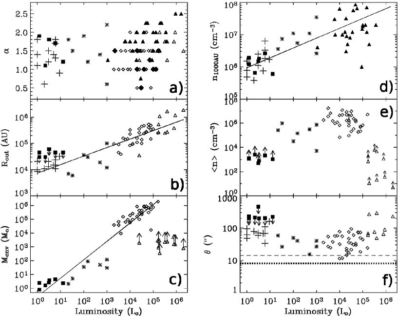
Figure 1: Plot of physical quantities within the envelopes surrounding low-, intermediate, and high-mass protostars as a function of their bolometric luminosity. Each symbol represents a different group of sources as follows: crosses: Jørgensen et al. (2002); filled squares: Shirley et al. (2002); stars: this study and Crimier et al. (2009a, b); diamonds: Williams et al. (2005); filled diamonds: Van der Tak et al. (2000) ; triangles: Hatchell & van der Tak (2003); filled triangles: Mueller et al. (2002). Symbols with arrows represent upper/lower limits. The solid line represents the linear fit of the points obtained when the correlation is significant (Table 6). The dashed line and the dotted line on panel f) represent the angular resolution of the SCUBA maps at 850 and 450 $\mu$m, respectively, which were used in all the in the studies reported in this panel.

Figure 2: Plot of the density at 10 K as function of the bolometric luminosity of a sample of low- and intermediate mass protostars. Data are from Jørgensen et al. (2002), (crosses), and the present study, (stars).

Physical parameter	Linear correlation	Number of	Probability for	Linear fit
vs. Log(L⊙)	coefficient	objects	a chance correlation	slope
Log($\alpha$)	0.12	107	1.	$--$
Log(Rout)	0.90	60	10-20	0.3
Log(Menv)	0.96	46	10-22	1.3
Log(n1000AU)	0.72	56	10-8	0.3
Log($<$n$>$)	0.25	39	0.4	$--$
Log(n10K)	-0.26	18	0.5	$--$
Log($\theta$)	0.88	60	10-19	-6$\times$10-3

Table 6: Linear correlation coefficients and probability for a chance correlation between the pair of parameters plotted on Fig. 1 and 2.

4.2 The problem of the underestimated 24 $\mu$m flux

As mentioned in the previous sections, our modelling fails to reproduce the observed flux at 24$\mu$m by several orders of magnitude. This is certainly not due to a numerical problem in the computation but is rather a real problem: our model misses some key element. A possibility evoked in the literature is the presence of a large spherical cavity within the envelope (Jørgensen et al. 2005) which could significantly reduce the optical thickness at 24$\mu$m.

To check this hypothesis, we carried out a few tests using Cep E-mm as a representative case. The results of the tests are shown in Fig. 3. First, we added a 1800 AU radius cavity to the best-fit model of Table 4. As expected, the emission at 24 $\mu$m is increased by several orders of magnitude. However, this model badly fails to reproduce the brightness profiles (as shown in the figure). When a correct procedure is carried out that takes into account the variation in the brightness profiles, namely a minimisation of the $\chi 2$ varying all the envelope parameters, the situation returns to the original (best-fit) underestimation of the 24 $\mu$m flux. In fact, the introduction of a cavity leads to an increase of the density power law index, $\alpha$, to compensate for the resulting flattening of the model brightness profiles. As a result, the mass found in the outer envelope is lower so that the the overall dust optical depth must be increased to reproduce the integrated sub-millimetre fluxes. The dust opacity at 24 $\mu$m again becomes large and very little emission is able to escape at these wavelengths. These tests suggest that to solve the 24 $\mu$m flux problem it is necessary to have a low-opacity escape route for the 24 $\mu$m photons and a thick enough envelope to fit the brightness profiles : a simple cavity does not suffice.

Larsson et al. (2000, 2002) similarly found that the 24 $\mu$m flux is underestimated toward Serpens-FIRS1, using different tools and observations. In their first study, Larsson et al. used a 1D radiative transfer code assuming a spherical envelope model with a single power law density to reproduce the SED (similar to our approach). Their model underestimates the observed flux near 24 $\mu$m by several orders of magnitude. In their second study, they modelled the envelope with a 2D radiative transfer code, including a biconical cavity. This model reproduces fairly well the SED from the mid-IR to millimetre wavelengths, but again underestimates the observed flux at 24 $\mu$m by about a factor 3-10. The biconical cavity treatment alleviates but does not resolve the missing flux problem. Systematic studies of high-mass protostars by Van der Tak et al. (2000) and Williams et al. (2005) have led to similar results. Williams et al. (2005) modelled 36 high-mass protostellar objects at 850 $\mu$m, using DUSTY, as in the present study. The majority of their best-fits fail to reproduce the flux around 24 $\mu$m. They discuss the possibility of the contribution of high accretion rates, which would significantly increase the near-IR flux density (Osorio et al. 1999). Another contribution could come from the presence of circumstellar disks or the stochastic heating of small grains, which would alter the emission of the envelope and produce more short wavelength photons (e.g. Sellgren et al. 1983; Draine & Li 2001). However, the envelope is optically thick at these wavelengths, making the emission very sensitive to deviations from the assumed spherical shape. These additional processes still require a low-opacity escape route to exists (also mentioned by Van der Tak et al. 2000) to explain the missing 24 $\mu$m flux, for example a biconical cavity excavated by the outflow. Note that all the intermediate mass protostars studied here are associated with outflows, except OMC2-FIR4 for which the model indeed fits the observed flux at 24$\mu$m (see Crimier et al. 2009a). Finally, Van Der Tak et al. also suggest the possible evaporation of grain ice mantles close to the star, which would decrease the 20 $\mu$m optical depth by 30$\%$ (Ossenkopf & Henning 1994) in the T_dust $>$ 100 K region.

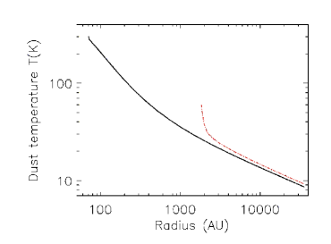
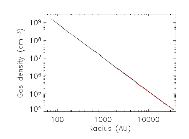
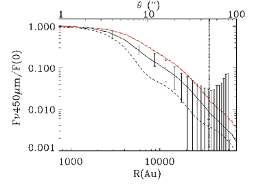
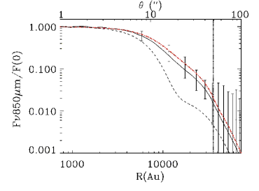
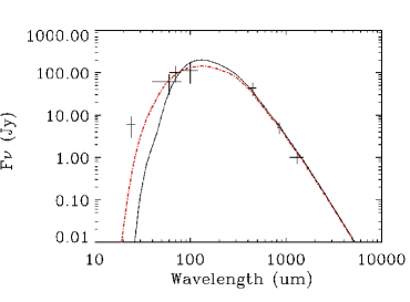
Figure 3: Cep E-mm physical structure, brightness profiles, and SED from the best-fit model (black solid lines) and after adding an 1800 AU radius cavity to the best-fit model (red dashed-dotted lines). The dust temperature and H₂ density profiles are reported in the upper left panel and upper right panel, respectively. The observed brightness profiles at 450 $\mu$m, 850 $\mu$m and the SED, observed and modelled, are shown in the middle left panel, the middle right panel, and the lower panel, respectively. The dashed lines represent the beam pattern of the telescope at 450 $\mu$m and 850 $\mu$m. The vertical black dotted lines show the outer radius of the best-fit model.

5 Conclusions

We have derived the physical structure of the envelopes of five IM protostars, with luminosities between 30 to 1000 L_⊙. The envelope dust density and temperature profiles were determined by means of the 1D radiative transfer code DUSTY, using all continuum observations from the literature. The analysis assumed that the density profiles follow a single index power law and obtained self-consistently the temperature profile. The best-fit envelope models well reproduce the observations, namely the sub-millimetre radial brightness profiles and the SED between $\sim$60 $\mu$m and 1.3 mm, for each source. However, the model underestimates the 24$\mu$m emission by several orders of magnitude. We ran test models to better understand what ingredient is missing and conclude that a “simple” cavity is not enough to reproduce the 24$\mu$m observations. Apparently, the missing ingredient is a low-opacity escape route plus a warm dust contribution inside the envelope (circumstellar disc, warm outflow-excavated cavity…).

The gas density and temperature profiles were derived by assuming a constant dust-to-gas ratio and by computing the gas thermal balance at each point within the envelope. Because the gas equilibrium temperature strongly depends on the water abundance in the interiors of the envelopes, we also computed the expected water emission for each source. We found that the gas and dust are thermally coupled across the envelope with differences less than 5 K in three out of five sources. In IC1396 N BIMA 2 and NGC7129 FIRS 2 the gas is colder than the dust by at most 40 K, in a small region just where the icy mantles are predicted to sublimate. The predicted water line fluxes are consistent with the upper limits derived by the ISO observations.

One of the major goals of the present study was to “use” the IM protostars as a bridge between the low- and high-mass protostars with the hope that this will aid our understanding of the star formation process at either end. When comparing the characteristics derived by the modelling of the envelopes of low-, intermediate, and high-mass protostars, it appears that there is a smooth transition between the various groups. This suggests that there are basically no different triggers or processes between these mass regimes. The power law index $\alpha$ is similar in all three groups of objects. The majority of the sources have $\alpha$ between 1.5 and 2. This is consistent with the theory of isothermal collapse from an initially singular isothermal sphere, the so-called inside-out expansion-wave collapse (Shu 1977). Regardless of the mass group, a few sources have $\alpha$ lower than 1.5, pointing perhaps to the collapse of an initially logotropic, virialised sphere (Lizano & Shu 1989, McLaughlin 96, and McLaughlin 97). Finally, the luminosity (mass) of the star depends on the size of the envelope, but does not depend on the density at a given temperature (for example at 10 K or 100 K).

Acknowledgements. We warmly thank Patrick Hennebelle for helpful discussions. One of us (N.Crimier) is supported by a fellowship of the Ministère de l’Enseignement Supérieur et de la Recherche. We acknowledge the financial support by PPF and the Agence Nationale pour la Recherche (ANR), France (contract ANR-08-BLAN-0225). The James Clerk Maxwell Telescope is operated by the Joint Astronomy Centre on behalf of the Science and Technology Facilities Council of the United Kingdom, the Netherlands Organisation for Scientific Research, and the National Research Council of Canada. This paper has been partially supported by MICINN, within the programme CONSOLIDER INGENIO 2010, under grant ”Molecular Astrophysics: The Herschel and Alma Era – ASTROMOL” ( ref.: CSD2009-00038) Doug Johnstone is supported by a Natural Sciences and Engineering Research Council of Canada (NSERC) Discovery Grant.

Appendix A Results for individual sources

A.1 CB3-mm

A.1.1 Source background

The CB3 Bok globule is located at $\sim$ 2.5 kpc (Launhardt & Henning 1997; Wang et al. 1995) on the near side of the Perseus arm of the Galaxy. Using ISO data, Launhardt et al. (1998) carried out a multi-wavelength study of the CB3 globule and derived a total mass and bolometric luminosity of the order of 400 M_☉ and $\sim$ 1000 L_☉, respectively, for the entire globule. The globule hosts $\sim$ 40 NIR sources, 22 of which are likely low- and intermediate mass protostars in different stages of evolution (Launhardt et al. 1998; Yun & Clemens 1995, 1994). CB3-mm, the brightest millimetre source in the globule, was first detected by Launhardt & Henning (1997) and subsequently observed in the sub-millimetre by Huard et al. (2000). The high luminosity of the source evaluated by Launhardt & Henning (1997), L $\sim$ 900 L_☉, suggests that CB3-mm is an intermediate mass object. A recent interferometric study by Fuente et al. (2007) showed that CB3-mm contains two compact cores at 3 mm separated by 0.3 pc ($\sim$ 0.43″). Yun & Clemens (1994) also detected a molecular bipolar outflow in CO, elongated in the northeast-southwest direction, associated with H₂O masers (de Gregorio-Monsalvo et al. 2006). This outflow has been mapped in various molecular lines by Codella & Bachiller (1999), who concluded that it originates from CB3-mm. The same authors concluded that CB3-mm is probably a Class 0 source. In the present study we re-evaluated the luminosity of this object, L $\sim$ 1000 L_☉, making CB3-mm an intermediate mass protostar.

A.1.2 Analysis

The continuum maps used for the CB3-mm analysis are presented in Fig. 4. The maps at 450 $\mu$m and 850 $\mu$m were obtained on 1997 December 18 as a part of project m96bi28 and on 1998 August 10 as a part of project m98bc21, respectively. The flux profiles obtained at each wavelength are shown in Fig. 5. The Spitzer observations were obtained on the 20th September 2004 as part of the programme “Comparative Study of Galactic and Extragalactic HII Regions” (AOR: 63, PI: James R. Houck). The integrated fluxes used for the analysis are reported in Table 2 and in Fig. 5. The fluxes at 70 $\mu$m, 450 $\mu$m and 850 $\mu$m were obtained by integration over a $\sim$ 50″radius. The uncertainty ellipse position of the IRAS observations are reported on the 450 $\mu$m maps in Fig. 4. Note that the map at 24 $\mu$m presents two sources separated by $\sim$12″, centred on the sub-millimetre source emission (see Fig. 4). Therefore, the flux $1.4\pm 0.8$ Jy at 24 $\mu$m was obtained by adding the integrated flux over the two sources separately. We also report on the SED the lower limits from Plateau de Bure (PdB) interferometric fluxes at 1.3 mm and 3 mm (Fuente et al. 2007).

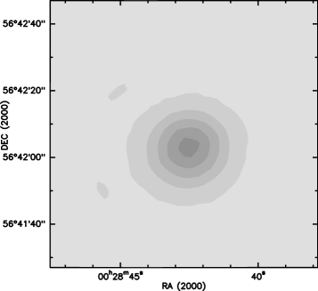
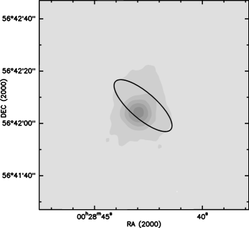
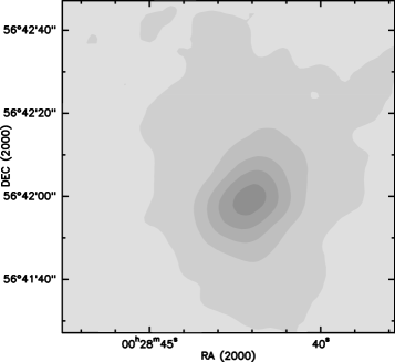
Figure 4: Continuum emission maps around CB3-mm at 24 $\mu$m (upper left panel), 70 $\mu$m (upper right panel), 450 $\mu$m (lower left panel), and 850 $\mu$m (lower right panel). The grey scale contours mark the continuum flux from 10 % to 90 % of the peak emission by steps of 20 %. The uncertainty ellipse position of the IRAS observations toward CB3-mm are represented by the ellipse in the 450 $\mu$m map.

A.1.3 Best-fit

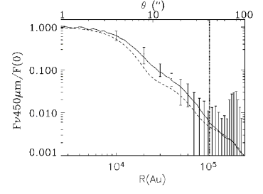
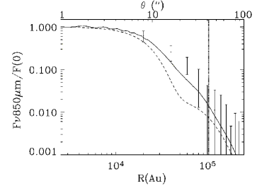
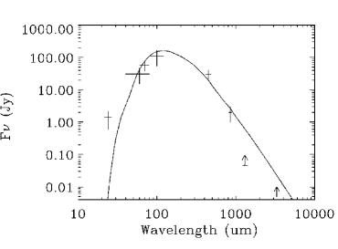
Figure 5: Observed brightness profiles at 450 $\mu$m (upper left panel), 850 $\mu$m (upper right panel) and SED (lower centred panel) toward CB3-mm. The solid lines report the best-fit model. The dashed lines represent the beam pattern of the telescope at 450 $\mu$m and 850 $\mu$m. The vertical dotted lines show the outer radius of the best-fit model (Table 4). The lower limits from Plateau de Bure (PdB) interferometric fluxes at 1.3 mm and 3 mm (Fuente et al. 2007) are also reported on the SED.

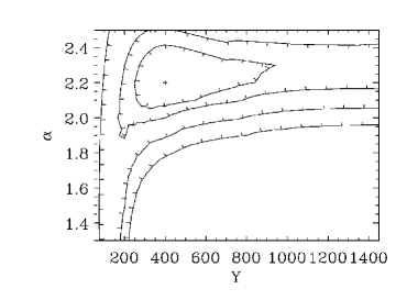
Figure 6: $\chi^{2}_{red}$ contour plots (Y,$\alpha$) for the CB3-mm model. In these computations, $\tau_{100}$ is equal to 5.8. The contours show the loci of the $\chi^{2}_{red}$ values equal to 1.1, 1.2, 1.5 and 2 times the minimum $\chi^{2}_{red}$ (10, 20, 50 and 100%). The cross shows the position of the best-fit.

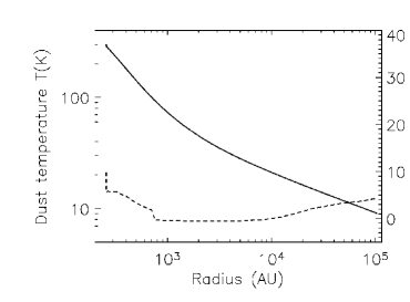
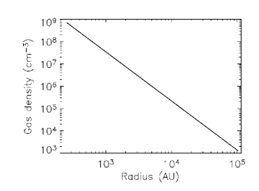
Figure 7: CB3-mm dust temperature (left panel) and H₂ density (right panel) profiles from the best-fit model. The dashed line represents the difference between the dust and gas temperature derived using X(H₂O)${}_{in}=$ 1$\times$10^-5 and X(H₂O)${}_{out}=$ 1$\times$10^-7 (scale on right axis).

Table 4 presents the set of parameters $\alpha$, Y, and $\tau_{100}$, which best reproduce the observations, and summarises some relevant physical quantities of the model. Figure 5 shows the best derived brightness profiles and SED against the observed ones, while Fig. 6 shows the $\chi^{2}$ contour plots. The dust density and temperature profiles of the best-fit model are reported in Fig. 7. Although the observed flux profiles and SED fluxes from 60 $\mu$m to 850 $\mu$m are well reproduced by the model, the observed flux at 24 $\mu$m is underestimated by about two orders of magnitude. The model agrees well with the lower limits from Plateau de Bure interferometric fluxes at 1.3 mm and 3 mm (Fuente et al. 2007), however.

The best-fit model, obtained with an $\alpha$ of 2.2, is the steepest among the five sources modelled in the paper and leads to a strong gradient in the density profile, from $\sim$ 10⁹ to $\sim$ 10³ cm^-3 with a density and radius at 100 K of 7.5$\times$10⁷ cm^-3 and 700 AU, respectively.

Although CB3-mm is the largest and brightest of the five sources investigated in this paper, its distance of 2500 pc makes it the least resolved source. Indeed, the brightness profiles at each wavelength presented in Fig. 5 are close to the beam patterns of the telescope, showing that the source is barely resolved. Consequently, the value of the envelope radius $r_{out}$ suffers a relatively large uncertainty. Considering the $\chi^{2}_{red}$ contour at 10% of the minimum $\chi^{2}_{red}$ (see Fig. 6) in order to estimate the uncertainty, we obtain $r_{out}$ = (1.0 $\pm^{1.3}_{3.9}$)$\times 10^{5}$ AU. On the contrary, the envelope column density is quite insensitive to $r_{out}$, due to the high power law index of the density profile. Finally, in minimising the $\chi_{SED}^{2}$, we also varied the source luminosity from 800 L_⊙ to 1200 L_⊙ and found that the best-fit is obtained with source luminosity equal to 1000 L_⊙.

A.2 Cep E-mm

A.2.1 Source background

Located in the Cepheus OB3 association at a distance of 730 pc (Sargent 1977; Crawford $\&$ Barnes 1970), Cepheus E is the second most massive and dense clump of this region (Few $\&$ Cohen 1983). Cepheus E hosts the source IRAS 23011+6126, which is associated with Cep E-mm, catalogued as a Class 0 protostar by Lefloch et al. (1996). Targeted by several continuum and lines studies, Cep E-mm has been observed with IRAS (Palla et al. 1993), IRAM 30m (Lefloch et al. 1996; Chini et al. 2001), SCUBA (Chini et al. 2001), ISO (Froebrich et al. 2003), and Spitzer (Noriega-Crespo et al. 2005). All these studies confirm the Class 0 status of Cep E-mm and constrain the total mass and bolometric luminosity of the source to 7–25 M_☉ and $\sim$ 80–120 L_☉, respectively. Finally, a bipolar molecular outflow, first reported by Fukui et al. (1989), is associated with Cep E-mm. The properties of the outflow have been thoroughly analysed by Eislöffel et al. (1996), Ayala et al. (2000), Moro-Martín et al. (2001), and Smith et al. (2003). The H₂ and [FeII] study by Eislöffel et al. (1996) shows a quadrapolar outflow morphology, suggesting that the driving source is a binary. This outflow morphology has been confirmed by sub-mm and near-IR observations (Ladd & Hodapp 1997), and by Spitzer observations (Noriega-Crespo et al. 2005).

A.2.2 Analysis

The continuum maps used for the Cep E-mm analysis are presented in Fig. 8. The maps at 450 $\mu$m and 850 $\mu$m were obtained in August 1997 as a part of the project m97bu87 and the observations are described in detail by Chini et al. (2001). The flux profiles obtained at each wavelength are shown in Fig. 9. The Spitzer observations were obtained on the 2003 September 29 as part of the programme “MIPS/IRAC imaging of protostellar jet HH 212” (AOR: 1063, PI: Alberto Noriega-Crespo) and are described in detail by Noriega-Crespo & Garnavich (2001). The integrated fluxes at 450 $\mu$m, 850 $\mu$m, and 1300 $\mu$m were retrieved from the literature (Chini et al. 2001). The uncertainty ellipse position of the IRAS observation is reported on the 450 $\mu$m map in Fig. 8. The fluxes at 24 $\mu$m and 70 $\mu$m were obtained by integration over a $\sim$ 30″and $\sim$ 60″radius, respectively. Note that to compute the flux uncertainties, we varied the integration radius of about 50% and found variations of $\mathrel{\hbox{\hbox to0.0pt{\hbox{\lower 4.0pt\hbox{$\sim$}}\hss}\hbox{$<$}}}$ 30%. The integrated fluxes used for the analysis are reported in Table 2 and in Fig. 9.

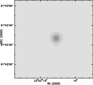
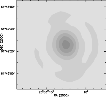
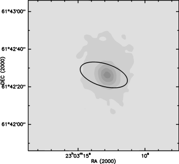
Figure 8: Continuum emission maps around Cep E-mm at 24 $\mu$m (upper left panel), 70 $\mu$m (upper right panel), 450 $\mu$m (lower left panel), and 850 $\mu$m (lower right panel). The grey scale contours mark the continuum flux from 10 % to 90 % of the peak emission in steps of 20 %. The uncertainty ellipse position of the IRAS observation toward Cep E-mm is reported on the 450 $\mu$m map.

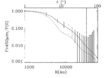
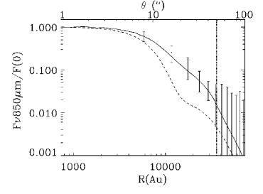
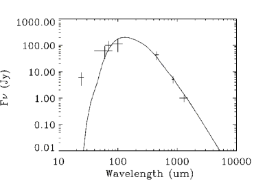
Figure 9: Observed brightness profiles at 450$\mu$m (upper left panel), 850 $\mu$m (upper right panel), and the SED (lower centred panel) toward Cep E-mm. The solid lines report the best-fit model (Table 4). The dashed lines represent the beam pattern of the telescope at 450 $\mu$m and 850 $\mu$m. The vertical dotted lines show the outer radius of the best-fit model.

A.2.3 Best-fit

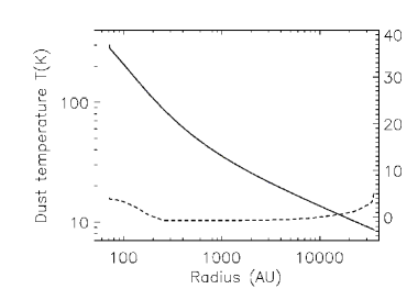
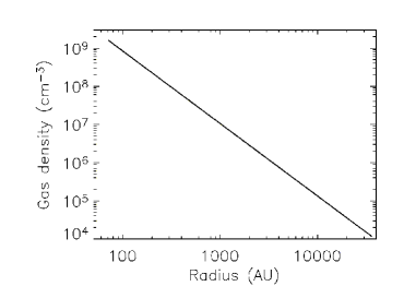
Figure 10: Cep E-mm dust temperature (left panel) and H₂ density (right panel) profiles from the best-fit model. The dashed line represents the difference between the dust and gas temperature derived using X(H₂O)${}_{in}=$ 1$\times$10^-5 and X(H₂O)${}_{out}=$ 1$\times$10^-7 (scale on right axis).

Table 4 presents the set of parameters $\alpha$, Y, and $\tau_{100}$, which best reproduce the observations, and summarises some relevant physical quantities of the model. Figure 9 shows the derived brightness profiles and SED against the observations. The dust density and temperature profiles of the best-fit model are reported in Fig. 10. Although the observed flux profiles and SED fluxes from 60 $\mu$m to 1300 $\mu$m are well reproduced by the model, the observed flux at 24 $\mu$m is underestimated by about $\sim$3 orders of magnitude. Similarly to CB3-mm, the envelope model derived for Cep E-mm with an $\alpha$ of 1.9 is very peaked, leading to a strong gradient in the density profile, from $\sim$ 10⁹ to $\sim$ 10⁴ cm^-3 with a density and radius at 100 K of 2.0$\times$10⁸ cm^-3 and 223 AU, respectively. Considering the $\chi^{2}_{red}$ contour at 10% of the minimum $\chi^{2}_{red}$ in order to estimate the uncertainty, we obtained $r_{out}$ = (3.6$\pm$0.7) $\times 10^{4}$ AU. Finally, in minimising the $\chi_{SED}^{2}$, we also varied the source luminosity from 70 L_⊙ to 130 L_⊙ and found the best-fit for a source luminosity equal to 100 L_⊙.

A.3 IC1396 N BIMA 2

A.3.1 Source background

IC1396 N is a bright globule located 750 pc (Matthews 1979) from the Sun, near the border of the IC1396 extended HII region (Osterbrock 1957; Weikard et al. 1996) and at a projected distance of 11 pc north of the O6.5 star HD 206267 which ionises the region. IC1396 N is associated with the source IRAS21391+5802. Its strong submillimetre and millimetre continuum emission (Wilking et al. 1993; Sugitani et al. 2000; Codella et al. 2001), high-density gas (Serabyn et al. 1993; Cesaroni et al. 1999; Codella et al. 2001; Beltrán et al. 2004), and water maser emission (Felli et al. 1992; Tofani et al. 1995; Patel et al. 2000) reveal that IC1396 N is an active site of star formation. The bolometric luminosity is estimated to range from 235 L_☉ (Saraceno et al. 1996) to 440 L_☉ (Sugitani et al. 2000).

Using BIMA interferometric millimetre observations, Beltrán et al. (2002) detected three sources (BIMA 1, BIMA 2 and BIMA 3) deeply embedded in the globule. BIMA 2 has the strongest millimetre emission and is also the most massive object. The authors concluded that BIMA 2 is most likely an IM protostar, while BIMA 1, and BIMA 3, located at $\sim$15″west and south-east respectively, are less massive and/or more evolved. The recent studies by Neri et al. (2007) and Fuente et al. (2007), using Plateau de Bure interferometric observations, provide a detailed study of BIMA 2 and showed that BIMA 2 contains at least three dense cores separated by $\sim$1″.

Finally, the region presents an extended ($\sim$3 arcmin) CO bipolar outflow (Sugitani et al. 1989) which has been mapped by Codella et al. (2001). The study by Nisini et al. (2001), revealed several H₂ jets inside the region. A more recent analysis (Beltrán et al. 2002, 2004) shows that BIMA 1 and BIMA 2 are associated with north-south and east-west bipolar molecular outflows, respectively.

A.3.2 Analysis

The continuum maps used for the IC1396 N BIMA 2 analysis are presented in Fig. 11. The SCUBA maps were obtained in March 2002 as a part of the project m02au07. The brightness profiles (see Fig. 12) are derived excluding the regions contaminated by the presence of BIMA 1 and BIMA 3 (dashed regions in Fig. 11). The Spitzer observations were obtained in October 2004 as part of the programme “Star Formation in Bright Rimmed Clouds” (AOR: 202, PI: Giovanni Fazio). The integrated fluxes used for the analysis are reported in Table 2 and in Fig. 12. The integrated fluxes at 450 $\mu$m and 850 $\mu$m were obtained by integration over a $\sim$ 35″. We varied the integration radius from 20″to 90″, and found variations on the fluxes $\mathrel{\hbox{\hbox to0.0pt{\hbox{\lower 4.0pt\hbox{$\sim$}}\hss}\hbox{$<$}}}$ 30%. The large uncertainty in the integrated flux at 24 $\mu$m is due to the proximity of BIMA 3 (see 24 $\mu$m map in Fig. 11). Note that due to the large IRAS beams at 60 $\mu$m and 100 $\mu$m, BIMA 3 introduces significant spurious signal. We thus used the IRAS and 70 $\mu$m Spitzer fluxes as upper limits on the SED (Fig 12).

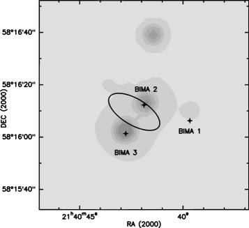
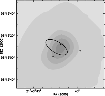
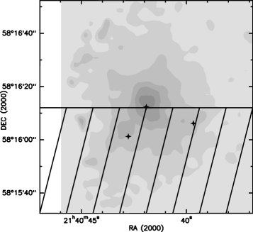
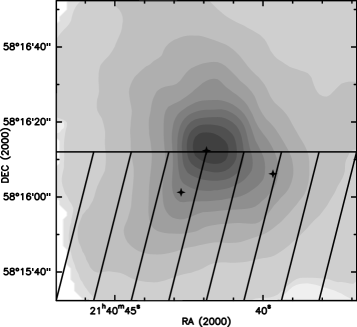
Figure 11: Continuum emission maps around IC1396 N BIMA 2 at 24 $\mu$m (upper left panel), 70 $\mu$m (upper right panel), 450 $\mu$m (lower left panel), and 850 $\mu$m (lower right panel). The grey scale contours mark the continuum flux from 10 % to 90 % of the peak emission by steps of 20 %. The positions of BIMA 1, BIMA 2 and BIMA 3, as well as the uncertainty ellipse position of the IRAS observations are reported on the 24 $\mu$m map. The dashed regions on the 450 $\mu$m and 850 $\mu$m maps mark the regions excluded to derive the flux profiles.

A.3.3 Best-fit

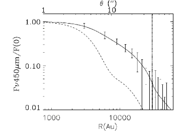
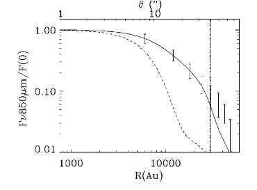
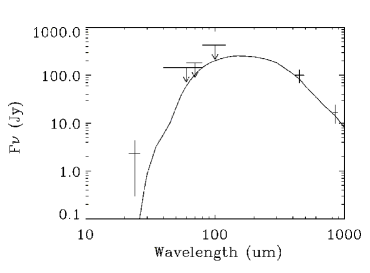
Figure 12: Observed brightness profiles at 450 $\mu$m (upper left panel), 850 $\mu$m (upper right panel) and the SED (lower centred panel) toward IC1396 N BIMA 2. The solid lines report the best-fit model (Table 4). The dashed lines represent the beam pattern of the telescope at 450 $\mu$m and 850 $\mu$m. The vertical dotted lines show the outer radius of the best-fit model. The IRAS and 70 $\mu$m Spitzer fluxes are used as upper limits on the SED.

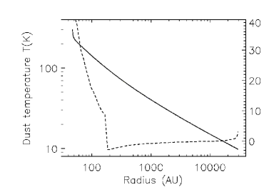
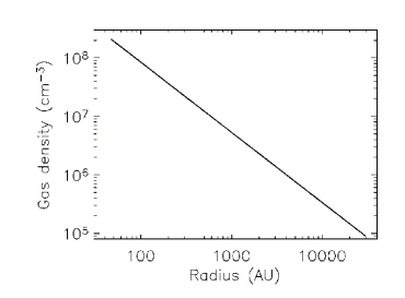
Figure 13: IC1396 N BIMA 2 dust temperature (left panel) and H₂ density (right panel) profiles from the best-fit model. The dashed line represents the difference between the dust temperature and the gas temperature derived using X(H₂O)${}_{in}=$ 1$\times$10^-5 and X(H₂O)${}_{out}=$ 1$\times$10^-7 (scale on right axis).

Table 4 presents the set of parameters $\alpha$, Y, and $\tau_{100}$, which best reproduce the observations, and summarises some relevant physical quantities of the model. Figure 12 shows the relevant derived brightness profiles and SED against the observations. The dust density and temperature profiles of the best-fit model are reported in Fig. 13. The observed flux profiles and SED fluxes at 450 $\mu$m and 850 $\mu$m are well reproduced by the model. Considering the IRAS and 70 $\mu$m Spitzer fluxes as upper limits (see Sect. A.3.2), the minimum $\chi_{SED}^{2}$ is obtained for a source luminosity equal to 150 L_⊙, similar to the value suggested by Beltrán et al. (2002). The observed flux at 24 $\mu$m is underestimated by about one order of magnitude. Considering the $\chi^{2}_{red}$ contour at 10% of the minimum $\chi^{2}_{red}$ to estimate the uncertainty, we obtained $r_{out}$ = (3.0$\pm$0.6) $\times 10^{4}$ AU. Note that we obtain similar results without subtracting the dashed region of Fig. 11, confirming the weak contribution of BIMA 1 and 3 to the submillimetre emission.

Finally, contrary to the previous sources, the gas temperature profile obtained for IC1396 N BIMA 2 is slightly decoupled from the dust temperature in the inner region (see Fig. 13). The origin of this thermal decoupling is discussed in detail in Crimier et al. (2009a). Briefly, the decoupling is due to a competition between the water abundance (the main coolant of the gas in the inner region) and the dust density, which mainly regulates the balance energy in the inner part of the envelope. This thermal decoupling is stronger in IC1396 N BIMA 2 (and NGC7129 FIRS 2) than in the other sources because of the lower density in the inner region. The thermal decoupling reaches a maximum value of about 40 K ($\sim$15% of T_dust) for an abundance of X(H₂O)${}_{in}=$ 1$\times$10^-5 and about 10 K for an abundance of X(H₂O)${}_{in}=$ 1$\times$10^-6.

A.4 NGC7129 FIRS 2

A.4.1 Source background

NGC7129 is a reflection nebula located in a complex and active molecular cloud (Hartigan & Lada 1985; Miranda et al. 1993) and estimated to be at a distance of 1250$\pm$50 pc (Shevchenko & Yakubov 1989) from the Sun. The region contains several Herbig AeBe stars, which illuminate the nebula. NGC7129 FIRS 2 has been detected in the far-infrared by Bechis et al. (1978) and Harvey et al. (1984). FIRS 2 is not detected at optical or near-infrared wavelengths. Its position coincides with a ¹³CO column density peak (Bechis et al. 1978) and a high-density NH₃ cloudlet (Guesten & Marcaide 1986). It is also close to an H₂O maser (Rodriguez et al. 1980). NGC7129 FIRS 2 has been classified as an IM Class 0 source by Eiroa et al. (1998), who carried out a multi-wavelength study of the continuum emission from 25 $\mu$m to 2000 $\mu$m. These authors estimate a total mass and bolometric luminosity of $\sim$ 6 M_☉ and $\sim$ 430 L_☉, respectively. In addition, Edwards $\&$ Snell (1983) detected a bipolar CO outflow associated with FIRS 2. The interferometric study of Fuente et al. (2001) has confirmed this bipolar outflow and pointed out a quadrapolar morphology to the flow. This quadrapolar morphology seems to be due to the superposition of two flows, FIRS 2-out 1 and FIRS 2-out 2, likely associated with FIRS 2 and a more evolved star (FIRS 2-IR), respectively. Finally, Fuente et al. (2005a, b) carried out an extensive chemical study of FIRS 2 providing the first detection of a hot core in an IM Class 0. Based on all these studies, FIRS 2 is considered the youngest IM object known at present.

A.4.2 Analysis

All the data and continuum maps used for the NGC7129 FIRS 2 analysis are reported in Table 2 and Fig. 14. T he maps at 450 $\mu$m and 850 $\mu$m were obtained on the 1998 August 26 as a part of the project M98BU24. We also used the flux profile and the integrated flux at 1300 $\mu$m extracted from the single dish map at 1300 $\mu$m, presented in Fuente et al. (2001). Following Greve et al. (1998), the beam at 1300 $\mu$m is assumed to be a combination of three Gaussian curves, with HPBWs of 11″, 125″, and 180″, with amplitude ratios of 0.975, 0.005, and 0.001, respectively. The Spitzer observations were obtained on the 2003 September 19 as part of the programme “Protostars and Proto-Brown Dwarfs in a Nearby Dark Cloud” (AOR: 34, PI: Tom Megeath). The integrated fluxes reported in Table 2 and in Fig. 15 were obtained by integration over a $\sim$ 40″radius. The IRAS integrated fluxes at 60 $\mu$m and 100 $\mu$m were taken from Eiroa et al. (1998).

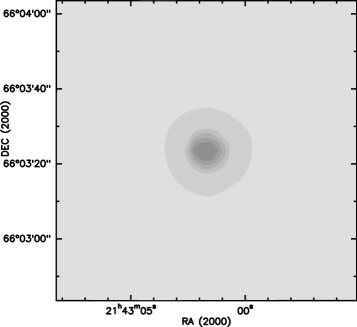
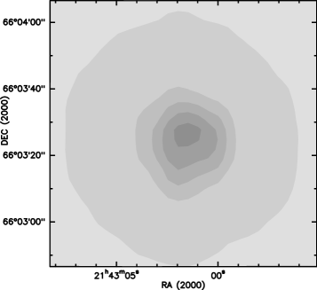
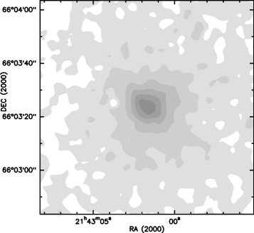
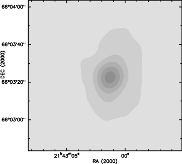
Figure 14: Continuum emission maps around NGC7129 FIRS 2 at 24 $\mu$m (upper left panel), 70 $\mu$m (upper right panel), 450 $\mu$m (middle left panel), 850 $\mu$m (middle right panel), and 1300 $\mu$m (lower centred panel). The grey scale contours mark the continuum flux from 10 % to 90 % of the peak emission by steps of 20 %.

A.4.3 Best-fit

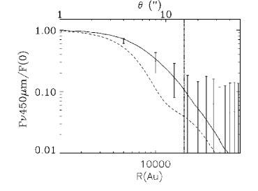
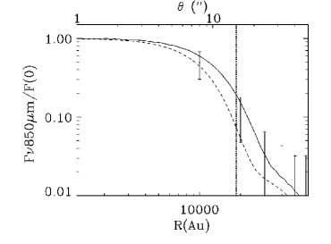
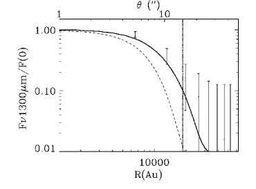
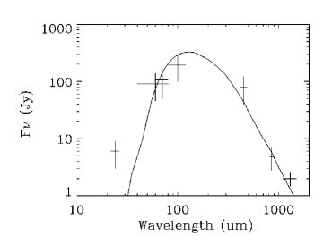
Figure 15: Observed brightness profiles at 450 $\mu$m (upper left panel), 850 $\mu$m (upper right panel), 1300 $\mu$m (lower left panel), and the SED (lower right panel) toward NGC7129 FIRS 2. The solid lines report the best-fit model (Table 4). The dashed lines represent the beam pattern of the telescope at 450 $\mu$m, 850 $\mu$m, 1300 $\mu$m. The vertical dotted lines show the outer radius of the best-fit model.

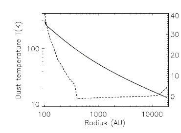
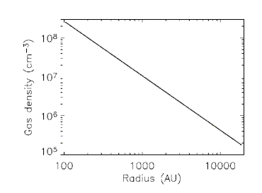
Figure 16: NGC7129 FIRS 2 dust temperature (left panel) and H₂ density (right panel) profiles from the best-fit model. The dashed line represents the difference between the dust and gas temperature derived using X(H₂O)${}_{in}=$ 1$\times$10^-5 and X(H₂O)${}_{out}=$ 1$\times$10^-7 (scale on right axis).

Table 4 presents the set of parameters $\alpha$, Y, and $\tau_{100}$, which best reproduce the observations, and summarises some relevant physical quantities of the model. Figure 15 shows the relevant derived brightness profiles and SED against the observations. The dust density and temperature profiles of the best-fit model are reported in Fig. 16. The observed flux profiles and SED fluxes from 60 $\mu$m to 850 $\mu$m are well reproduced by the model. In minimising the $\chi_{SED}^{2}$, we also varied the source luminosity from 400 L_⊙ to 600 L_⊙ and found the best-fit for a source luminosity equal to 500 L_⊙. The observed flux at 24 $\mu$m is underestimated by about two orders of magnitude. Considering the $\chi^{2}_{red}$ contour at 10% of the minimum $\chi^{2}_{red}$ to estimate the uncertainty, we obtained $r_{out}$ = (1.9$\pm$0.2) $\times 10^{4}$ AU.

Finally, similarly to IC1396 N BIMA 2, the gas temperature profile obtained in NGC7129 FIRS 2 is slightly decoupled from the dust temperature in the inner part (see Fig. 16).

A.5 Serpens FIRS 1

A.5.1 Source background

Since its recognition as a very active star forming region (Strom et al. 1974), the Serpens molecular cloud has been the target of many observational studies. Several studies have been dedicated to evaluate the distance of this cloud from the Sun, yielding a range of distances from $\sim$ 210 to 440 pc. Following the review by Eiroa et al. (2008), which reports and compares the distance results from all the different studies, we adopt a distance of $\sim$ 230$\pm$20 pc. Serpens is a young protocluster whose members are in many different evolutionary stages. About 100 embedded YSO, protostars, and prestellar clumps (Strom et al. 1976; Eiroa & Casali 1992; Casali et al. 1993; Hurt & Barsony 1996; Giovannetti et al. 1998; Testi & Sargent 1998; Kaas 1999), as well as molecular outflows (White et al. 1995; Wolf-Chase et al. 1998; Williams & Myers 2000) and H₂ emission (e.g. Eiroa et al. 1997; Herbst et al. 1997; Hodapp 1999) have been detected in this region.

Serpens FIRS 1 is located near the centre of the Serpens main core and is the most luminous object embedded in the cloud. Several continuum studies classify it as Class 0 source with a bolometric luminosity estimated to range from 46 L_☉ to 84 L_☉ (Harvey et al. 1984; Casali et al. 1993; Hurt & Barsony 1996; Larsson et al. 2000). The latest estimation of its luminosity suggests that Serpens FIRS 1 is on the low/intermediate mass protostar border. The envelope physical structure of Serpens FIRS 1 has been modelled by Hogerheijde et al. (1999) using millimetre interferometric observations of the continuum and molecular line observations. The Serpens FIRS 1 SED was first modelled by means of a spherical envelope 1D radiative transfer code by Larsson et al. (2000). Subsequently, Larsson et al. (2002) used a 2D radiative transfer code and a torus model to reproduce the SED and line observations from ISO. FIRS1 drives a molecular outflow, which is orientated at a position angle of 50 degrees, coincident with a triple radio source with symmetric lobes (Rodriguez et al. 1989).

A.5.2 Analysis

The continuum maps used for the Serpens FIRS 1 analysis are presented in Fig. 17. The SCUBA maps were obtained in January 1998 as a part of the project m97bc30. The flux profiles (see Fig. 18) are derived excluding the dashed regions in Fig. 17 to avoid the non-spherical extended emission. The Spitzer observations were obtained in October 2004 as part of the programme “From Molecular Cores to Planets, continued” (AOR: 174, PI: Neal Evans). The integrated fluxes used for the analysis are reported in Table 2 and in Fig. 18. The integrated fluxes from 70 $\mu$m to 850 $\mu$m were obtained by integration over a $\sim$ 40″. We also report on the SED the lower limits from Plateau de Bure (PdB) interferometric fluxes at 1.3 mm and 3 mm (Fuente et al. 2007).

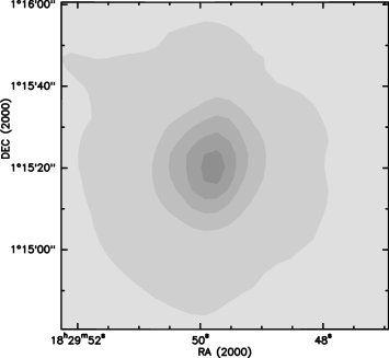
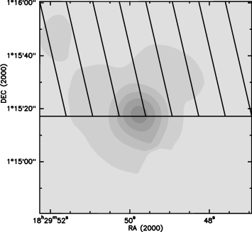
Figure 17: Continuum emission maps around Serpens FIRS 1 at 24 $\mu$m (upper left panel), 70 $\mu$m (upper right panel), 450 $\mu$m (lower left panel), and 850 $\mu$m (lower right panel). The grey scale contours mark the continuum flux from 10 % to 90 % of the peak emission by steps of 20 %. The dashed regions on the 450 $\mu$m and 850 $\mu$m show the regions excluded to derive the brightness profiles.

A.5.3 Best-fit

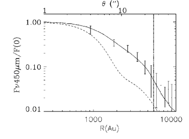
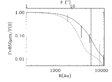
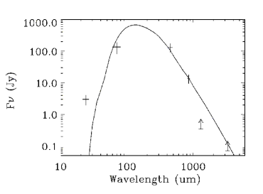
Figure 18: Observed brightness profiles at 450 $\mu$m (upper left panel), 850 $\mu$m (upper right panel) and the SED (lower centred panel) toward Serpens FIRS 1. The solid lines report the best-fit model (Table 4). The dashed lines represent the beam pattern of the telescope at 450 $\mu$m and 850 $\mu$m. The vertical dotted lines show the outer radius of the best-fit model. The lower limits from Plateau de Bure interferometric fluxes at 1.3 mm and 3 mm (Fuente et al. 2007) are also reported on the SED as lower limit.

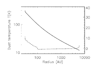
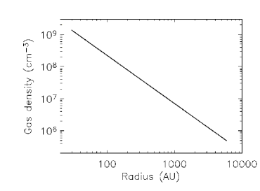
Figure 19: Serpens FIRS 1 dust temperature (left panel) and H₂ density (right panel) profiles from the best-fit model. The dashed line represents the difference between the dust temperature and the gas temperature derived using X(H₂O)${}_{in}=$ 1$\times$10^-5 and X(H₂O)${}_{out}=$ 1$\times$10^-7 (scale on right axis).

Table 4 presents the set of parameters $\alpha$, Y, and $\tau_{100}$, which best reproduce the observations, and summarises some relevant physical quantities of the model. Figure 18 shows the relevant derived brightness profiles and SED against the observations. The dust density and temperature profiles of the best-fit model are reported in Fig. 19. The model well reproduces the observed flux profiles and SED fluxes from 70 $\mu$m to 850 $\mu$m and agrees well with the lower limits from Plateau de Bure interferometric fluxes at 1.3 mm and 3 mm (Fuente et al. 2007). In minimising the $\chi_{SED}^{2}$, we also varied the source luminosity from 20 L_⊙ to 60 L_⊙ and found the best-fit for a source luminosity equal to 33 L_⊙. Note that the estimated value of the bolometric luminosity is much lower than the values derived in previous studies toward this source (Harvey et al. 1984; Casali et al. 1993; Hurt & Barsony 1996; Larsson et al. 2000). This is due to the adopted smaller distance to the source. Considering the $\chi^{2}_{red}$ contour at 10% of the minimum $\chi^{2}_{red}$ to estimate the uncertainty, we obtained $r_{out}$ = (5.9$\pm$0.3) $\times 10^{3}$ AU.

Hogerheijde et al. (1999) studied the envelope physical structure of Serpens FIRS 1 using interferometric continuum observations at OVRO at $\lambda=$ 3.4-1.4 mm and single-dish line observations from JCMT and CSO. They adopted a bolometric luminosity of 77 L_⊙ and fixed the outer radius of the envelope R${}_{out}=$ 8000 AU for a distance of 400 pc. Hogerheijde et al. (1999) derived an envelope with density profile index $\alpha=$ 2$\pm$0.5 in good agreement with our results. By scaling their results to the same distance adopted here (230 pc) their adopted luminosity, $\sim$ 25 L_⊙, and the envelope radius R${}_{out},\sim$ 4600 AU, are relatively consistant with our results (Table 4) : L $\sim$ 33 L_⊙, R${}_{out}\sim$ 5900 AU. Also their derived gas temperature profile slightly differs from ours: for example they obtained T${}_{gas}\sim$ 40 K at 200 AU while we obtained T${}_{gas}\sim$ 65 K. Larsson et al. (2000) studied the SED of Serpens FIRS 1, derived from the ISO LWS maps and photometric data between $\sim$ 1 and 10⁵ $\mu$m retrieved from the literature. These authors used i) a single temperature/optically thin approximation and ii) a radiative transfer model to analyse the SED. In their models they adopted a distance of 310 pc, a source diameter of 7″and a power law density profile index, $\alpha=$2. They succeeded in reproducing the SED between 40 $\mu$m and 3 mm. By scaling their results to the same distance adopted here (230 pc), they obtain a luminosity of $\sim$ 40 L_⊙, against our estimate of 33 L_⊙, and an envelope mass of 1.1-3.3 M_⊙, against our estimate of 5 M_⊙. However, as noticed by the authors themselves, their mass estimate is rather a lower limit, given the optically thin approximation they used.

Finally, the observed flux at 24 $\mu$m is underestimated by about two orders of magnitude. This phenomenon is also observed in the Larsson et al. (2002, 2000) studies. We discuss the situation at 24 $\mu$m in more detail in the the following section, Sect. 4.

References

- Alonso-Albi et al. (2009) Alonso-Albi et al. 2009, in prep
- Andre et al. (1993) Andre, P., Ward-Thompson, D., & Barsony, M. 1993, ApJ, 406, 122
- Andre et al. (2000) Andre, P., Ward-Thompson, D., & Barsony, M. 2000, Protostars and Planets IV, 59
- Ayala et al. (2000) Ayala, S., Noriega-Crespo, A., Garnavich, P. M., et al. 2000, AJ, 120, 909
- Bechis et al. (1978) Bechis, K. P., Harvey, P. M., Campbell, M. F., & Hoffmann, W. F. 1978, ApJ, 226, 439
- Beltrán et al. (2004) Beltrán, M. T., Girart, J. M., Estalella, R., & Ho, P. T. P. 2004, A&A, 426, 941
- Beltrán et al. (2002) Beltrán, M. T., Girart, J. M., Estalella, R., Ho, P. T. P., & Palau, A. 2002, ApJ, 573, 246
- Beuther et al. (2007) Beuther, H., Churchwell, E. B., McKee, C. F., & Tan, J. C. 2007, in Protostars and Planets V, ed. B. Reipurth, D. Jewitt, & K. Keil, 165–180
- Boogert et al. (2004) Boogert, A. C. A., Pontoppidan, K. M., Lahuis, F., et al. 2004, ApJS, 154, 359
- Bottinelli (2006) Bottinelli, S. 2006, PhD thesis, University of Hawai’i at Manoa
- Casali et al. (1993) Casali, M. M., Eiroa, C., & Duncan, W. D. 1993, A&A, 275, 195
- Caux et al. (1999) Caux, E., Ceccarelli, C., Castets, A., et al. 1999, A&A, 347, L1
- Ceccarelli et al. (2007) Ceccarelli, C., Caselli, P., Herbst, E., Tielens, A. G. G. M., & Caux, E. 2007, in Protostars and Planets V, ed. B. Reipurth, D. Jewitt, & K. Keil, 47–62
- Ceccarelli et al. (1996) Ceccarelli, C., Hollenbach, D. J., & Tielens, A. G. G. M. 1996, ApJ, 471, 400
- Ceccarelli et al. (2003) Ceccarelli, C., Maret, S., Tielens, A. G. G. M., Castets, A., & Caux, E. 2003, A&A, 410, 587
- Cesaroni et al. (1999) Cesaroni, R., Felli, M., & Walmsley, C. M. 1999, A&AS, 136, 333
- Chandler et al. (1998) Chandler, C. J., Barsony, M., & Moore, T. J. T. 1998, MNRAS, 299, 789
- Chini et al. (2001) Chini, R., Ward-Thompson, D., Kirk, J. M., et al. 2001, A&A, 369, 155
- Codella & Bachiller (1999) Codella, C. & Bachiller, R. 1999, A&A, 350, 659
- Codella et al. (2001) Codella, C., Bachiller, R., Nisini, B., Saraceno, P., & Testi, L. 2001, A&A, 376, 271
- Crimier et al. (2009a) Crimier, N., Ceccarelli, C., Lefloch, B., & Faure, A. 2009a, A&A, 506, 1229
- Crimier et al. (2009b) Crimier, N., Ceccarelli, C., Maret, S., et al. 2009b, A&A, submitted
- de Gregorio-Monsalvo et al. (2006) de Gregorio-Monsalvo, I., Gómez, J. F., Suárez, O., et al. 2006, AJ, 132, 2584
- Di Francesco et al. (1997) Di Francesco, J., Evans, II, N. J., Harvey, P. M., et al. 1997, ApJ, 482, 433
- Doty & Neufeld (1997) Doty, S. D. & Neufeld, D. A. 1997, ApJ, 489, 122
- Draine & Li (2001) Draine, B. T. & Li, A. 2001, ApJ, 551, 807
- Eiroa & Casali (1992) Eiroa, C. & Casali, M. M. 1992, A&A, 262, 468
- Eiroa et al. (2008) Eiroa, C., Djupvik, A. A., & Casali, M. M. 2008, The Serpens Molecular Cloud, ed. B. Reipurth, 693–+
- Eiroa et al. (1998) Eiroa, C., Palacios, J., & Casali, M. M. 1998, A&A, 335, 243
- Eiroa et al. (1997) Eiroa, C., Palacios, J., Eisloffel, J., Casali, M. M., & Curiel, S. 1997, in IAU Symposium, Vol. 182, Herbig-Haro Flows and the Birth of Stars, ed. B. Reipurth & C. Bertout, 103P–+
- Eislöffel et al. (1996) Eislöffel, J., Smith, M. D., Davis, C. J., & Ray, T. P. 1996, AJ, 112, 2086
- Evans et al. (2001) Evans, II, N. J., Rawlings, J. M. C., Shirley, Y. L., & Mundy, L. G. 2001, ApJ, 557, 193
- Faure et al. (2007) Faure, A., Crimier, N., Ceccarelli, C., et al. 2007, A&A, 472, 1029
- Faure & Josselin (2008) Faure, A. & Josselin, E. 2008, A&A, 492, 257
- Felli et al. (1992) Felli, M., Palagi, F., & Tofani, G. 1992, A&A, 255, 293
- Flower et al. (2006) Flower, D. R., Pineau Des Forêts, G., & Walmsley, C. M. 2006, A&A, 449, 621
- Frerking et al. (1982) Frerking, M. A., Langer, W. D., & Wilson, R. W. 1982, ApJ, 262, 590
- Froebrich et al. (2003) Froebrich, D., Smith, M. D., Hodapp, K.-W., & Eislöffel, J. 2003, MNRAS, 346, 163
- Fuente et al. (2007) Fuente, A., Ceccarelli, C., Neri, R., et al. 2007, A&A, 468, L37
- Fuente et al. (2005a) Fuente, A., Neri, R., & Caselli, P. 2005a, A&A, 444, 481
- Fuente et al. (2001) Fuente, A., Neri, R., Martín-Pintado, J., et al. 2001, A&A, 366, 873
- Fuente et al. (2005b) Fuente, A., Rizzo, J. R., Caselli, P., Bachiller, R., & Henkel, C. 2005b, A&A, 433, 535
- Fukui et al. (1989) Fukui, Y., Iwata, T., Mizuno, A., Ogawa, H., & Takaba, H. 1989, Nature, 342, 161
- Giovannetti et al. (1998) Giovannetti, P., Caux, E., Nadeau, D., & Monin, J.-L. 1998, A&A, 330, 990
- Gomez et al. (1993) Gomez, M., Hartmann, L., Kenyon, S. J., & Hewett, R. 1993, AJ, 105, 1927
- Gondhalekar & Wilson (1975) Gondhalekar, P. M. & Wilson, R. 1975, A&A, 38, 329
- Greve et al. (1998) Greve, A., Kramer, C., & Wild, W. 1998, A&AS, 133, 271
- Guesten & Marcaide (1986) Guesten, R. & Marcaide, J. M. 1986, A&A, 164, 342
- Habing (1968) Habing, H. J. 1968, BAIN, 19, 421
- Hartigan & Lada (1985) Hartigan, P. & Lada, C. J. 1985, ApJS, 59, 383
- Harvey et al. (1984) Harvey, P. M., Wilking, B. A., & Joy, M. 1984, ApJ, 278, 156
- Hatchell & van der Tak (2003) Hatchell, J. & van der Tak, F. F. S. 2003, A&A, 409, 589
- Hennebelle & Fromang (2008) Hennebelle, P. & Fromang, S. 2008, A&A, 477, 9
- Herbst et al. (1997) Herbst, T. M., Beckwith, S. V. W., & Robberto, M. 1997, ApJ, 486, L59+
- Hillenbrand & Hartmann (1998) Hillenbrand, L. A. & Hartmann, L. W. 1998, ApJ, 492, 540
- Hodapp (1999) Hodapp, K. W. 1999, AJ, 118, 1338
- Hogerheijde et al. (1999) Hogerheijde, M. R., van Dishoeck, E. F., Salverda, J. M., & Blake, G. A. 1999, ApJ, 513, 350
- Huard et al. (2000) Huard, T. L., Weintraub, D. A., & Sandell, G. 2000, A&A, 362, 635
- Hurt & Barsony (1996) Hurt, R. L. & Barsony, M. 1996, ApJ, 460, L45+
- Ivezic & Elitzur (1997) Ivezic, Z. & Elitzur, M. 1997, MNRAS, 287, 799
- Jørgensen et al. (2007) Jørgensen, J. K., Bourke, T. L., Myers, P. C., et al. 2007, ApJ, 659, 479
- Jørgensen et al. (2005) Jørgensen, J. K., Lahuis, F., Schöier, F. L., et al. 2005, ApJ, 631, L77
- Jørgensen et al. (2002) Jørgensen, J. K., Schöier, F. L., & van Dishoeck, E. F. 2002, A&A, 389, 908
- Kaas (1999) Kaas, A. A. 1999, AJ, 118, 558
- Krumholz et al. (2005) Krumholz, M. R., McKee, C. F., & Klein, R. I. 2005, ApJ, 618, L33
- Ladd & Hodapp (1997) Ladd, E. F. & Hodapp, K.-W. 1997, ApJ, 474, 749
- Larsson et al. (2002) Larsson, B., Liseau, R., & Men’shchikov, A. B. 2002, A&A, 386, 1055
- Larsson et al. (2000) Larsson, B., Liseau, R., Men’shchikov, A. B., et al. 2000, A&A, 363, 253
- Launhardt et al. (1998) Launhardt, R., Evans, II, N. J., Wang, Y., et al. 1998, ApJS, 119, 59
- Launhardt & Henning (1997) Launhardt, R. & Henning, T. 1997, A&A, 326, 329
- Lefloch et al. (1996) Lefloch, B., Eisloeffel, J., & Lazareff, B. 1996, A&A, 313, L17
- Li & Shu (1996) Li, Z. & Shu, F. H. 1996, ApJ, 472, 211
- Lizano & Shu (1989) Lizano, S. & Shu, F. H. 1989, ApJ, 342, 834
- Mannings & Sargent (1997) Mannings, V. & Sargent, A. I. 1997, ApJ, 490, 792
- Mannings & Sargent (2000) Mannings, V. & Sargent, A. I. 2000, ApJ, 529, 391
- Matthews (1979) Matthews, H. I. 1979, A&A, 75, 345
- McKee & Tan (2003) McKee, C. F. & Tan, J. C. 2003, ApJ, 585, 850
- McLaughlin & Pudritz (1996) McLaughlin, D. E. & Pudritz, R. E. 1996, ApJ, 469, 194
- McLaughlin & Pudritz (1997) McLaughlin, D. E. & Pudritz, R. E. 1997, ApJ, 476, 750
- Miranda et al. (1993) Miranda, L. F., Eiroa, C., & Gomez de Castro, A. I. 1993, A&A, 271, 564
- Moro-Martín et al. (2001) Moro-Martín, A., Noriega-Crespo, A., Molinari, S., et al. 2001, ApJ, 555, 146
- Motte & André (2001) Motte, F. & André, P. 2001, A&A, 365, 440
- Mueller et al. (2002) Mueller, K. E., Shirley, Y. L., Evans, II, N. J., & Jacobson, H. R. 2002, ApJS, 143, 469
- Neri et al. (2007) Neri, R., Fuente, A., Ceccarelli, C., et al. 2007, A&A, 468, L33
- Nisini et al. (2001) Nisini, B., Massi, F., Vitali, F., et al. 2001, A&A, 376, 553
- Noriega-Crespo & Garnavich (2001) Noriega-Crespo, A. & Garnavich, P. M. 2001, AJ, 122, 3317
- Noriega-Crespo et al. (2005) Noriega-Crespo, A., Moro-Martin, A., Carey, S., et al. 2005, in ESA Special Publication, Vol. 577, ESA Special Publication, ed. A. Wilson, 453–454
- Osorio et al. (1999) Osorio, M., Lizano, S., & D’Alessio, P. 1999, ApJ, 525, 808
- Ossenkopf & Henning (1994) Ossenkopf, V. & Henning, T. 1994, A&A, 291, 943
- Osterbrock (1957) Osterbrock, D. E. 1957, ApJ, 125, 622
- Palla et al. (1993) Palla, F., Cesaroni, R., Brand, J., et al. 1993, A&A, 280, 599
- Parise et al. (2005) Parise, B., Ceccarelli, C., & Maret, S. 2005, A&A, 441, 171
- Patel et al. (2000) Patel, N. A., Greenhill, L. J., Herrnstein, J., et al. 2000, ApJ, 538, 268
- Rodriguez et al. (1989) Rodriguez, L. F., Curiel, S., Moran, J. M., et al. 1989, ApJ, 346, L85
- Rodriguez et al. (1980) Rodriguez, L. F., Moran, J. M., Ho, P. T. P., & Gottlieb, E. W. 1980, ApJ, 235, 845
- Sandell & Weintraub (2001) Sandell, G. & Weintraub, D. A. 2001, ApJS, 134, 115
- Saraceno et al. (1996) Saraceno, P., Ceccarelli, C., Clegg, P., et al. 1996, A&A, 315, L293
- Schöier et al. (2002) Schöier, F. L., Jørgensen, J. K., van Dishoeck, E. F., & Blake, G. A. 2002, A&A, 390, 1001
- Schreyer et al. (2002) Schreyer, K., Henning, T., van der Tak, F. F. S., Boonman, A. M. S., & van Dishoeck, E. F. 2002, A&A, 394, 561
- Sellgren et al. (1983) Sellgren, K., Werner, M. W., & Dinerstein, H. L. 1983, ApJ, 271, L13
- Serabyn et al. (1993) Serabyn, E., Guesten, R., & Mundy, L. 1993, ApJ, 404, 247
- Shevchenko & Yakubov (1989) Shevchenko, V. S. & Yakubov, S. D. 1989, Soviet Astronomy, 33, 370
- Shirley et al. (2002) Shirley, Y. L., Evans, II, N. J., & Rawlings, J. M. C. 2002, ApJ, 575, 337
- Shu (1977) Shu, F. H. 1977, ApJ, 214, 488
- Shu & Adams (1987) Shu, F. H. & Adams, F. C. 1987, in IAU Symposium, Vol. 122, Circumstellar Matter, ed. I. Appenzeller & C. Jordan, 7–22
- Smith et al. (2003) Smith, M. D., Froebrich, D., & Eislöffel, J. 2003, ApJ, 592, 245
- Stahler et al. (1986) Stahler, S. W., Palla, F., & Salpeter, E. E. 1986, ApJ, 302, 590
- Strom et al. (1974) Strom, S. E., Grasdalen, G. L., & Strom, K. M. 1974, ApJ, 191, 111
- Strom et al. (1976) Strom, S. E., Vrba, F. J., & Strom, K. M. 1976, AJ, 81, 638
- Sugitani et al. (1989) Sugitani, K., Fukui, Y., Mizuni, A., & Ohashi, N. 1989, ApJ, 342, L87
- Sugitani et al. (2000) Sugitani, K., Matsuo, H., Nakano, M., Tamura, M., & Ogura, K. 2000, AJ, 119, 323
- Testi et al. (1999) Testi, L., Palla, F., & Natta, A. 1999, A&A, 342, 515
- Testi & Sargent (1998) Testi, L. & Sargent, A. I. 1998, ApJ, 508, L91
- Tofani et al. (1995) Tofani, G., Felli, M., Taylor, G. B., & Hunter, T. R. 1995, A&AS, 112, 299
- Troscompt et al. (2009) Troscompt, N., Faure, A., Wiesenfeld, L., Ceccarelli, C., & Valiron, P. 2009, A&A, 493, 687
- van der Tak et al. (1999) van der Tak, F. F. S., van Dishoeck, E. F., Evans, II, N. J., Bakker, E. J., & Blake, G. A. 1999, ApJ, 522, 991
- Van der Tak et al. (2000) Van der Tak, F. F. S., van Dishoeck, E. F., Evans, II, N. J., & Blake, G. A. 2000, ApJ, 537, 283
- Vastel et al. (2000) Vastel, C., Caux, E., Ceccarelli, C., et al. 2000, A&A, 357, 994
- Visser et al. (2002) Visser, A. E., Richer, J. S., & Chandler, C. J. 2002, AJ, 124, 2756
- Wang et al. (1995) Wang, Y., Evans, II, N. J., Zhou, S., & Clemens, D. P. 1995, ApJ, 454, 217
- Weikard et al. (1996) Weikard, H., Wouterloot, J. G. A., Castets, A., Winnewisser, G., & Sugitani, K. 1996, A&A, 309, 581
- White et al. (1995) White, G. J., Casali, M. M., & Eiroa, C. 1995, A&A, 298, 594
- Wilking et al. (1993) Wilking, B., Mundy, L., McMullin, J., Hezel, T., & Keene, J. 1993, AJ, 106, 250
- Williams & Myers (2000) Williams, J. P. & Myers, P. C. 2000, ApJ, 537, 891
- Williams et al. (2005) Williams, S. J., Fuller, G. A., & Sridharan, T. K. 2005, A&A, 434, 257
- Wolf-Chase et al. (1998) Wolf-Chase, G. A., Barsony, M., Wootten, H. A., et al. 1998, ApJ, 501, L193+
- Young et al. (2003) Young, C. H., Shirley, Y. L., Evans, II, N. J., & Rawlings, J. M. C. 2003, ApJS, 145, 111
- Yun & Clemens (1994) Yun, J. L. & Clemens, D. P. 1994, AJ, 108, 612
- Yun & Clemens (1995) Yun, J. L. & Clemens, D. P. 1995, AJ, 109, 742