Reverse Line Graph Construction: The Matrix Relabeling Algorithm MARINLINGA Versus Roussopoulos’s Algorithm

Abstract

We propose a new algorithm MARINLINGA for reverse line graph computation, i.e., constructing the original graph from a given line graph. Based on the completely new and simpler principle of link relabeling and endnode recognition, MARINLINGA does not rely on Whitney’s theorem while all previous algorithms do. MARINLINGA has a worst case complexity of $O(N^{2})$, where $N$ denotes the number of nodes of the line graph. We demonstrate that MARINLINGA is more time-efficient compared to Roussopoulos’s algorithm, which is well-known for its efficiency.

1 Introduction

The line graph $l\left(G\right)$ of a graph $G$ is a graph in which every node corresponds to a link of $G$ and two nodes are adjacent if and only if their corresponding links are adjacent in $G$ (two links are adjacent if they are incident to the same node). The graph $G$ is called the original or root graph of $l\left(G\right)$. There exist examples of line graphs from social network. Given $M$ clubs and $N$ students at an university, every student joins two clubs. Each student has different choices (we assume that there are enough clubs). We define two networks $G_{1}$ and $G_{2}$. The $M$ clubs are the nodes of $G_{1}$ and two nodes are adjacent if two clubs have the same student as their member. The $N$ students are the nodes of $G_{2}$ and two nodes are adjacent if two students belong to the same club Clearly, $G_{2}$ is the line graph of $G_{1}$. Such pairs $\left(G_{1},G_{2}\right)$ are common in on-line social networks like Facebook, Twitter and etc., where users join the special groups where they share the same interest with others. Computing the line graph of a graph and constructing the original graph of a line graph also play an important role in link partitioning of communities [6][1][5][10], bond percolation threshold predictions [18], and it also enables us to compare the properties of a random line graph [9] and its original graph.

The following formula [14] can be used to compute the adjacency matrix of the line graph $l\left(G\right)$ of a graph $G$,

$$A_{l\left(G\right)}=\left(R^{T}R\right)_{L\times L}-2I$$ (1)

where $R$ is the incidence matrix of the undirected graph $G$. If link $j$ is incident to node $i$, the entry $r_{ij}$ of $R$ is $1$, otherwise $0$. In each column there are exactly two $1$-entries.

Constructing the original graph is far more complex than computing the line graph. Before constructing the original graph from a given graph, it is important to know whether the graph is a line graph. Up till now, the following criteria for a graph to be a line graph exist in the literature:

• A graph is a line graph if and only if it is possible to find a collection of cliques in the graph, partitioning all the links, such that each node belongs to at most two of the cliques (some of the cliques can be a single node) and two cliques share at most one node [7]. If the graph is not $K_{3}$, there can be only one partition of this type.

• A graph is a line graph if and only if it does not have the complete bipartite graph $K_{1,3}$ as an induced subgraph, and if two odd triangles have a common link, the subgraph induced by their nodes is the complete graph $K_{4}$ [15].

• A graph is a line graph if and only if none of the nine forbidden subgraphs (see Figure 1) is an induced subgraph of it [2].

• A graph is not a line graph [14] if the smallest eigenvalue of the adjacency matrix $\left(\ref{adjacency_matrix_line_graph}\right)$ is smaller than $-2$.

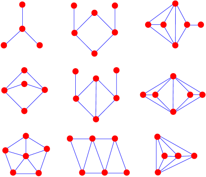
Figure 1: The nine forbidden subgraphs for line graphs [2].

The complete graph on three nodes $K_{3}$ is a line graph, which has two different original graphs, $K_{3}$ and $K_{1,3}$ (Figure 21 (b)). Except for $K_{3}$, Whitney’s theorem [17][7] states that, all line graphs have only one original graph (isomorphic graphs are considered as the same graph). Based on the above criteria and Whitney’s theorem, several algorithms for constructing the original graph have been proposed [8][12][11][3]. Among those algorithms, Roussopoulos’s [12] and Lehot’s [8] solutions are worth mentioning here.

Roussopoulos’s algorithm starts with choosing an arbitrary link in the input graph and calculating the number of triangles containing this link. Depending on this value the starting cell is determined. The starting cell is a complete graph $K_{m}$; if $m=2$ it is a link; if $m=3$ a triangle that contains the starting link. Having a starting cell of the input graph, the algorithm of Roussopoulos continues to find a clique, which is deleted. In addition, in each step the vertices of the clique are labeled by a group number. One node in a line graph cannot be assigned to more than two groups (otherwise it is not a line graph). The nodes of the original graph are those partitions and all nodes are assigned to exactly one partition. In the constructed graph there is a link between two nodes, if the nodes are assigned to partitions that have a non-empty intersection. The approach of Roussopoulos is based on finding the largest connected components and sequentially the number of triangles that contain this link. Theoretically finding the largest connected component is, however, an $NP$-complete problem [16]. Lehot’s solution is based on the characterization of line graphs by Van Rooij and Wilf [8][15].

In this paper, we propose a new algorithm, the MAtrix Relabeling INverse LINe Graph Algorithm, in short MARINLINGA, that constructs the original graph given the line graph. MARINLINGA does not explicitly rely on Whitney’s theorem, as all previous companion algorithms, but uses link relabeling and endnode recognition in a new way. Via extensive simulation analysis, we have compared MARINLINGA with Roussopoulos’s algorithm. We demonstrate that MARINLINGA consumes less CPU running time. The algorithms are tested on the same machine and we use the same input line graphs for both algorithms.

2 Link adjacency matrix (LAM) and line graph

Two nodes of a graph are said to be adjacent if there is a link directly connecting them. The adjacency matrix $A$ of a graph contains all information of node adjacency: if node $i$ and node $j$ are adjacent, the entry $a_{ij}=1$, otherwise $a_{ij}=0$. Similarly, two links are adjacent if they are incident to the same node.

Definition 1

The link adjacency matrix (LAM) $C$ of a graph $G$ with $N_{G}$ nodes and $L_{G}$ links is the $L_{G}\times L_{G}$ symmetric matrix with the entry $c_{ij}=1$ if link $i$ and link $j$ of $G$ are adjacent, else $c_{ij}=0$.

The line graph $l\left(G\right)$ of the graph $G$ has $N_{l\left(G\right)}$ nodes and $L_{l\left(G\right)}$ links, and consequently we have $L_{G}=N_{l\left(G\right)}$. According to the definitions of the line graph and the LAM, evidently, the LAM $C$ of $G$ is equal to the adjacency matrix $A_{l\left(G\right)}$ of $l\left(G\right)$,

$$C=A_{l\left(G\right)}$$ (2)

Due to Whitney’s theorem and ignoring isomorphisms, for any graph except $K_{3}$ and $K_{1,3}$, one can construct the graph exclusively from its LAM. Usually, the (node) adjacency matrix is used to represent a graph. Here we use the LAM to specify any graph, except for $K_{3}$ and $K_{1,3}$. Constructing the original graph of a line graph is equivalent to converting a graph representation from the LAM to the adjacency matrix. By constructing the original graph directly from the line graph, confusion will arise concerning the links in the original graph and the nodes in the line graph. By introducing the concept of LAM, we can avoid confusion and facilitate the description of our algorithm MARINLINGA.

3 Properties of the LAM

For a simple (undirected, unweighted and without self-loops) graph $G\left(N_{G},L_{G}\right)$ with $N_{G}$ nodes and $L_{G}$ links, the LAM $C$ has more constraints than the corresponding adjacency matrix $A$, besides being symmetric and containing only $0$ and $1$ entries.

A link $i$ has two endnodes, the left endnode $i^{+}$ and the right endnode $i^{-}$. Link $j$ also has endnodes $j^{+}$ and $j^{-}$. There are four configurations where link $i$ is adjacent to link $j$, as shown in Figure 2. For each single pair of links, the LAM only indicates whether they are adjacent. If they are adjacent, we still do not know in which of the four possible configurations this pair of links is adjacent. Fortunately, by combining the adjacency relation of $3$ or more links, we can determine the configuration of those links.

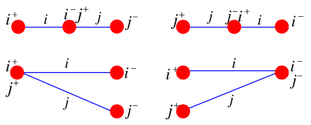
Figure 2: The four possible configurations in which link $i$ is adjacent to link $j$.

Definition 2

If $m$ links ($m\geq 2$) are adjacent to link $i$ and incident to the same endnode of link $i$, these $m$ links are pairwise adjacent.

Definition 3

The links, which are adjacent to link $i$, are defined as the neighboring links of link $i$.

Definition 4

The links incident to the left endnode $i^{+}$ of a link $i$ are defined as the left-neighboring links of $i$, and the links incident to the right endnode $i^{-}$ are defined as the right-neighboring links of $i$.

If we can recognize the link adjacency pattern of a link and its neighboring links, we can specify LAM entirely.

Figure 3 (a) depicts an example of a link and its neighboring links. The link $i$ has $5$ left neighboring links at its left endnode $i^{+}$, denoted as $i_{+1},\cdots,i_{+5}$, and $4$ right neighboring links at its right endnode $i^{-}$, denoted as $i_{-1},\cdots,i_{-4}$. The link adjacency pattern of these $10$ links is shown in Figure 3 (b). In the link adjacency pattern, the labels of the left-neighboring links $i_{+1},\cdots,i_{+5}$ are larger than link $i$, and smaller than the right-neighboring links $i_{-1},\cdots,i_{-4}$.

Given the configuration of link $i$ and its neighboring links, the corresponding link adjacency pattern conforms to the following rules:

1. the left-neighboring links (such as $i_{+1},\cdots,i_{+5}$ in the example of Figure 3 (a)) are incident to the same endnode $i^{+}$, and are said (Definition 2) to be pairwise adjacent. Similarly, the right-neighboring links (such as $i_{-1},\cdots,i_{-4}$ in the example of Figure 3 (a)) are also pairwise adjacent. This explains the two all-$1$-triangles (surrounded by the dashed lines) in Figure 3 (b), the upper one corresponding to $i^{+}$ and the second triangle corresponding to pairwise adjacent links $i_{-1},\cdots,i_{-4}$.

2. Since there is at most one link between two nodes (multi-links are forbidden), each of the left-neighboring links can be adjacent to at most one right neighboring link and vice versa. Hence in Figure 3 (b), there exists at most one $1$-entry in each row/column of the submatrix in yellow.

We summarize this observation:

Criterion 5

If the given link adjacency pattern has the following features, it is the link adjacency pattern of a link $i$ and its neighboring links (the labels of the left-neighboring links are larger than link $i$, and smaller than the right-neighboring links),

• All entries of the first row are $1$-entries;

• The triangle bounded by the $\left(n_{i^{+}}+1\right)$th column (including the $\left(n_{i^{+}}+1\right)$th column) is an all-$1$-triangle, where $n_{i^{+}}$ denotes the number of the left-neighboring links of link $i$ and $n_{i^{+}}\geq 3$;

• There is at most one $1$-entry in each row/column of the submatrix, which is from the $2$nd to the $\left(n_{i^{+}}+1\right)$th row and from the $\left(n_{i^{+}}+2\right)$th to the $\left(n_{i^{+}}+n_{i^{-}}+2\right)$th column, where $n_{i^{-}}$ denotes the number of the right-neighboring links;

• The triangle bounded by the $\left(n_{i^{+}}+2\right)$th row (including the $\left(n_{i^{+}}+2\right)$th row) is an all-$1$-triangle.

Figure 3: (a) The configuration of a link $i$ and its neighboring links. (b) The corresponding link adjacency pattern. there is at most one $1$-entry in each row/column of the submatrix in yellow. If all the entries in green and magenta are $1$-entries, the entries of the triangle in white must be also $1$-entries.

Theorem 6

Consider three links $i$, $j$ and $k$ are pairwise adjacent. If each of the other $m$ links is adjacent to all the three links $i$, $j$ and $k$, then all the $m+3$ links are pairwise adjacent.

Proof. The three links $i$, $j$ and $k$ are pairwise adjacent and the configuration of $i$, $j$ and $k$ can be $K_{3}$ or $K_{1,3}$, as shown in Figure 21 (b). If the configuration is $K_{3}$, other links can be adjacent to at most two of $i$, $j$ and $k$. However, if the other $m$ links are adjacent to $i$, $j$ and $k$, the configuration of $i$, $j$ and $k$ must be $K_{1,3}$, and $i$, $j$ and $k$ have a common endnode. Since each of the $m$ links is adjacent to $i$, $j$ and $k$, the common endnode of $i$, $j$ and $k$ must be also an endnode of each of the $m$ links. According to Definition 2, all these $m+3$ links are pairwise adjacent.   

In Figure 3 (b), links $i$, $i_{+1}$ and $i_{+2}$ are pairwise adjacent, as shown by entries in green. Links $i_{+3}$, $i_{+4}$ and $i_{+5}$ are adjacent to $i$, $i_{+1}$ and $i_{+2}$, as shown by entries in magenta. By Theorem 6, links $i$, $i_{+1}$, $i_{+2}$, $i_{+3}$, $i_{+4}$ and $i_{+5}$ are pairwise adjacent.

3.1 The basic forbidden link adjacency patterns in a LAM

Figure 4 (a) depicts the smallest forbidden link adjacency pattern in a LAM. The configuration of links $i$, $j$ and $k$ is a path on four nodes. Since link $i$ has neighboring links at both of its two endnodes, and if link $r$ is adjacent with link $i$, then link $r$ must be also adjacent with link $j$ or $k$. Hence, the pattern in Figure 4 (a) will not appear in a LAM.

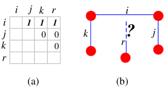
Figure 4: The smallest forbidden link adjacency pattern.

There are $6$ forbidden link adjacency patterns of links $i$, $j$, $k$, $r$ and $t$, as shown in Figure 6. Since the number of the left-neighboring links of link $i$ is smaller than $3$, we cannot use Criterion 5 to prove that the $6$ link adjacency patterns are forbidden. However, Figure 5, which exhibits the possible configurations of the link adjacency patterns of links $i$, $j$, $k$ and $r$, will facilitate the proof that the $6$ link adjacency patterns in Figure 6 are forbidden.

The link adjacency pattern of links $i$, $j$, $k$ and $r$ in Figure 6 (a), (b) and (c) are the same as the link adjacency pattern of links $i$, $j$, $k$ and $r$ in Figure 5 (a). There are only two possible configurations of this link adjacency pattern. As we can observe in Figure 5 (a), it is impossible to have a new link $t$ which is only adjacent with link $i$, or only adjacent with links $i$ and $j$, or adjacent with all of $i$, $j$, $k$ and $r$. Hence, the patterns in Figure 6 (a), (b) and (c) are forbidden. In the same way, we observe that the patterns in Figure 6 (d), (e) and (f) are also forbidden.

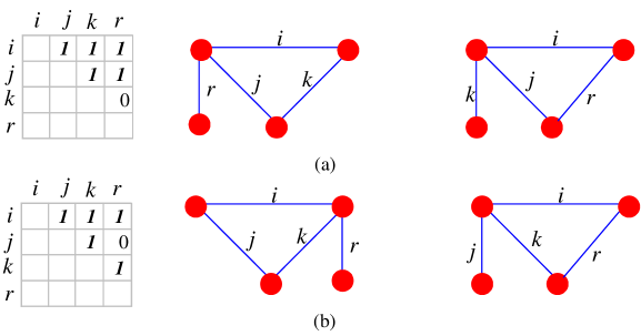
Figure 5: The possible configurations for two link adjacency patterns of $4$ links. This figure helps to prove that the patterns of $5$ links in Figure 6 are forbidden.

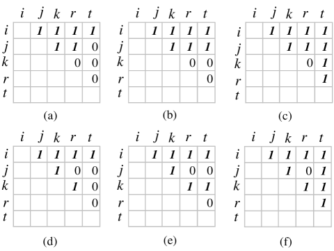
Figure 6: The forbidden link adjacency patterns of $5$ links.

When the number of the left-neighboring links of link $i$ is not smaller than $3$ (which implies that the number of $1$-entries in the first all-$1$-triangle is not smaller than $6$), we can use Criterion 5 to determine whether a link adjacency pattern is forbidden.

4 The matrix relabeling inverse line graph algorithm (MARINLINGA)

MARINLINGA is the algorithm that we designed to compute the original graph of a line graph, given the adjacency matrix of that line graph.

As explained in Section 2, the adjacency matrix $A_{l\left(G\right)}$ of $l\left(G\right)$ is equal to the LAM $C_{G}$ of $G$. Constructing the original graph of a line graph, is equivalent to constructing a graph given the LAM of that graph. MARINLINGA only deals with the upper triangle of the given LAM $C$.

4.1 Matrix relabeling

The matrix relabeling algorithm rearranges the LAM $C$ in such a way that the left and right neighboring links of the first link can be recognized via Theorem 6 and the construction algorithm can work efficiently. In each column there are some $1$-entries (red dots). If after relabeling the top $1$-entries of all the columns are connected by a curve, the curve should be nonincreasing. For example, by the LAM $C$ of a graph with $50$ links in Figure 7 (a), we can only determine which links are adjacent to the first link, without any information about which endnode of the first link that the neighboring links are incident to. Fortunately, according to Theorem 6, the relabeled LAM $C$ in Figure 7 (b) tells that links $2$-$5$ are the left-neighboring links of the first link and links $6$-$10$ are the right-neighboring links.

Figure 7: Matrix relabelling on the LAM $C$ of a graph with $50$ links. The red dots represent $1$-entries. (a) Before relabelling; (b) After relabelling.

Let us first introduce the meaning of swapping the labels of two links in a LAM $C_{L_{G}\times L_{G}}$. The entry $c_{ij}$ indicates whether links $i$ and $j$ are adjacent. Swapping the labels of links $j$ and $k$ ($j<k$) implies that links which are previously adjacent to link $j$ are now adjacent to link $k$, and links which are previously adjacent to link $k$, are now adjacent to link $j$, but the adjacency relation between links $j$ and $k$ is the same as before, namely the entry $c_{jk}$ of $C_{L_{G}\times L_{G}}$ is unchanged. Hence, swapping the labels of links $j$ and $k$ ($j<k)$ means to swap the entries $c_{ij}$ and $c_{ik}$ for $i=1,2,\cdots,j-1$ (shown in the example of Figure 8 in green), the entries $c_{ji}$ and $c_{ik}$ for $i=j+1,\cdots,k-1$ (in magenta), the entries $c_{ji}$ and $c_{ki}$, $i=k+1,\cdots,L_{G}-1,L_{G}$ (in yellow).

Algorithm 1 $C\Leftarrow SwapLabel(C,j,k)$

1:  for $i=1$ to $j-1$ do

2:     $swap(c_{ij},c_{ik})$

3:  end for

4:  for $i=j+1$ to $k-1$ do

5:     $swap(c_{ji},c_{ik})$

6:  end for

7:  for $i=k+1$ to $L_{G}$ do

8:     $swap(c_{ji},c_{ki})$

9:  end for

Lines 1-3 of the metacode of Algorithm 1 swap the entries $c_{ji}$ and $c_{ik}$, $i=j+1,\cdots,k-1$, and lines 4-6 swap the entries $c_{ji}$ and $c_{ik}$, $i=j+1,\cdots,k-1$, and lines 7-9 swap the entries $c_{ji}$ and $c_{ki}$, $i=k+1,\cdots,L_{G}-1,L_{G}$. The code $swap\left(c_{ij},c_{ik}\right)$ of line 2 is equivalent to the codes: $t=c_{ij}$; $c_{ij}=c_{ik}$; $c_{ik}=t$.

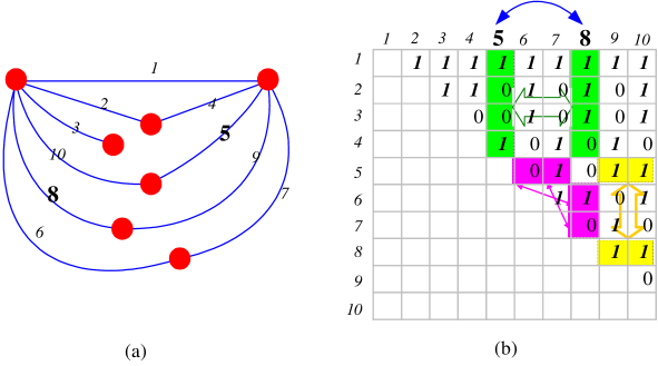
Figure 8: The illustration of swapping the labels of link $5$ and $8$. The entries in green, magenta and yellow ought to be swapped respectively.

Next, we will explain the matrix relabeling algorithm. We will first give an example showing how the matrix relabeling algorithm relabels the LAM $C$ in Figure 7 (a) into the matrix in Figure 7 (b). In the first row of the matrix in Figure 7 (a) there are $9$ 1-entries in total. There are $6$ 0-entries from $c_{1,2}$ to $c_{1,10}$ and $6$ 1-entries from $c_{1,11}$ to $c_{1,50}$: $c_{1,3}=c_{1,5}=c_{1,6}=c_{1,8}=c_{1,9}=c_{1,10}=0$ and $c_{1,13}=c_{1,15}=c_{1,18}=c_{1,19}=c_{1,24}=c_{1,40}=1$. We swap the labels of links $3$ and $13$, links $5$ and $15$, links $6$ and $18$, links $8$ and $19$, links $9$ and $24$, links $10$ and $40$ by Algorithm 2 and the LAM $C$ is shown in Figure 9. In the second row, there are $3$ 1-entries from $c_{2,3}$ to $c_{2,10}$. There are $2$ 0-entries from $c_{2,3}$ to $c_{2,5}$ and $2$ 1-entries from $c_{2,6}$ to $c_{2,10}$: $c_{2,4}=c_{2,5}=0$ and $c_{2,6}=c_{2,9}=1$. We swap the labels of links $4$ and $6$, links $5$ and $9$. By similar operations, we relabel the LAM $C$ into the order shown in Figure 7 (b).

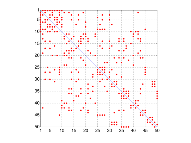
Figure 9: The LAM $C$ after the relabeling of the first row.

Algorithm 2 $C\Leftarrow GroupLabelSwapping(C,u,k,a,b)$

1:  $m\Leftarrow 0$

2:  for $i=u+1$ to $a+u$ do

3:     if $c_{ki}=0$ then

4:        $m\Leftarrow m+1$

5:        $X_{m}\Leftarrow i$

6:     end if

7:  end for

8:  $m\Leftarrow$ $0$

9:  for $i=a+u+1$ to $b$ do

10:     if $c_{ki}=1$ then

11:        $m\Leftarrow m+1$

12:        $Y_{m}\Leftarrow i$

13:     end if

14:  end for

15:  for $i=1$ to $m$ do

16:     $C\Leftarrow SwapLabel(C,X_{i},Y_{i})$

17:  end for

Now we give the general description of the matrix relabeling algorithm. In the $k$th row of $C$, Lines 1-7 of Algorithm 2 store the value of $i$ in $X$ when the entry $c_{ki}$ is $0$, $i=u+1,\cdots,a+u$. Lines 8-14 store the value of $i$ in $Y$ when the entry $c_{ki}$ is $1$, $i=a+u+1,\cdots,b$. If $a={\textstyle\sum\limits_{i=u+1}^{b}}c_{ki}$, $X$ and $Y$ have the same number of elements. Lines 15-17 swap the labels of $X_{i}$ and $Y_{i}$, where $X_{i}$ and $Y_{i}$ are the $i$th element of $X$ and $Y$ respectively. For instance in Figure 8 (b), if we take $u=2$, $k=2$, $b=10$ and $a={\textstyle\sum\limits_{i=3}^{10}}c_{2i}$ $=5$, by Algorithm 2, $X=\left[\begin{array}[c]{cc}5&7\end{array}\right]^{T},Y=\left[\begin{array}[c]{cc}8&10\end{array}\right]^{T}$, the labels of links $5$ and $8$, $7$ and $10$ are swapped respectively.

Algorithm 3 $(C,s_{1},s_{2},s_{3})\Leftarrow MatrixRelabeling(C)$

1:  $s_{1}\Leftarrow$ the sum of $c_{1i}$, where $i=2$ to $L_{G}$

2:  $C\Leftarrow GroupLabelSwapping(C,1,1,s_{1},L_{G})$

3:  $s_{2}\Leftarrow$ the sum of $c_{2i}$, where $i=3$ to $s_{1}+1$

4:  $C\Leftarrow GroupLabelSwapping(C,2,2,s_{2},s_{1}+1)$

5:  $s_{3}\Leftarrow$ the sum of $c_{3i}$, where $i=4$ to $s_{2}+2$

6:  $C\Leftarrow GroupLabelSwapping(C,3,3,s_{3},s_{2}+2)$

7:  $\bar{s}\Leftarrow s_{1}+1$

8:  $k\Leftarrow 2$

9:  while $\bar{s}<L_{G}$ and $k\leq L_{G}$ do

10:     $s\Leftarrow$ the sum of $c_{ki}$, where $i=\bar{s}+1$ to $L_{G}$

11:     $C\Leftarrow GroupLabelSwapping(C,\bar{s},k,s,L_{G})$

12:     $k\Leftarrow k+1$

13:     $\bar{s}\Leftarrow\bar{s}+s$

14:  end while

Lines 1-2 of Algorithm 3 make the neighboring links of link $1$ have the smaller labels than the other links. By lines 3-4, the labels of the links which are adjacent to both link $1$ and $2$ are smaller than those of the remaining links. Further, lines 5-6 let the labels of the links which are adjacent to all of links $1$, $2$ and $3$ are smaller than those of the remaining links. Lines 7-14 make that the labels of the links which are adjacent to link $i$ but not adjacent to links $1,\cdots,i-1$, are smaller than the labels of the links which are not adjacent to link $1,\cdots,i$, for $i=2,\cdots,L_{G}$. Figure 7 and 10 show examples of $C$ before and after matrix relabeling.

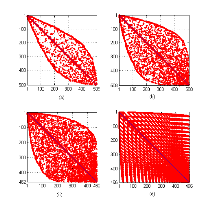
Figure 10: The relabeled $C$ of four ER random graphs $G\left(N,p\right)$: (a) $N=350$, $p=\frac{\log\left(N\right)}{2N}$; (b) $N=200$, $p=\frac{\log\left(N\right)}{N}$; (c) $N=100$, $p=\frac{2\log\left(N\right)}{N}$; (d) $N=32$, $p=1$, where $p=\frac{\log\left(N\right)}{N}$ is the threshold probability for the connectivity of the graph.

Let $s_{1}={\textstyle\sum\limits_{i=2}^{L_{G}}}c_{1i}$, $s_{2}={\textstyle\sum\limits_{i=3}^{s_{1}+1}}c_{2i}$ and $s_{3}={\textstyle\sum\limits_{i=4}^{s_{2}+2}}c_{3i}$. After relabeling by Algorithm 3, the given LAM $C$ satisfies:

• For $i=2,\cdots,s_{1}+1$, $c_{1i}=1$; and for $i=s_{1}+2,\cdots,L_{G}$, $c_{1i}=0$.

• For $i=3,\cdots,s_{2}+2$, $c_{2i}=1$ if $s_{2}\geq 1$; and for $i=s_{2}+3,\cdots,s_{1}+1$, $c_{2i}=0$ if $s_{1}\geq s_{2}+2$.

• For $i=4,\cdots,s_{3}+3$, $c_{3i}=1$ if $s_{3}\geq 1$; and for $i=s_{3}+4,\cdots,s_{2}+2$, $c_{3i}=0$ if $s_{2}\geq s_{3}+2$.

• If link $j$ ($j\geq s_{1+1}$) is adjacent to link $i$ but not adjacent to links $1,2,\cdots,i-1$ ($i\geq 2$), and link $k$ ($k\geq s_{1+1}$) is not adjacent to all of links $1,2,\cdots,i$ ($i\geq 2$), then $j<k$.

If $s_{3}\geq 1$ (which implies that $s_{2}\geq 2$ and $s_{1}\geq 3$), according to Theorem 6, links $2,3,\cdots,s_{3}+3$ are the left-neighboring links of links $1$ and the links $s_{3}+4,\cdots,s_{1}+1$ are the right-neighboring links of link $1$, as illustrated in the example of Figure 11 where $s_{1}=9$ and $s_{3}=3$.

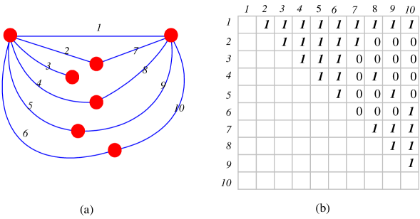
Figure 11: The LAM (a) relabeled by Algorithm 3 and its corresponding graph (b).

4.2 Construction algorithm

The construction algorithm converts the relabeled $C$ into the matrix $E_{2\times L_{G}}$, where the entries $e_{1i}$ and $e_{2i}$ denotes the two endnodes of link $i$. During the process of the construction, the zero entries of $E_{2\times L_{G}}$ mean that the endnodes have not been determined yet.

Section 4.2.1 will first show an example of graph construction, and section 4.2.2 and 4.2.3 will describe the general construction algorithm.

4.2.1 An example of graph construction from $C$

From the given LAM $C$ in Figure 7 (b), we deduce that the graph has $50$ links. Based on the LAM $C$, we will determine the endnodes of the $50$ links. The construction consists of the following steps:

1. Let nodes $1$ and $2$ be the endnodes of link $1$. According to Theorem 6, node $1$ is also the endnode of links $2$-$5$ and node $2$ is also the endnode of links $6$-$10$, as shown in Figure 12 (a) and equation $\left(\ref{Eq_construction_example_init}\right)$ below, where the numbers above the matrix are the link numbers.

   11111222220⋯020000000000⋯0​]\begin{array}[c]{c}\\ E=\end{array}\begin{array}[c]{c}\\ \left[\begin{array}[c]{c}\\ \\ \end{array}\right.\end{array}\begin{tabular}[c]{ccccccccccccc}${\footnotesize 1}$&${\footnotesize 2}$&${\footnotesize 3}$&${\footnotesize 4}$&${\footnotesize 5}$&${\footnotesize 6}$&${\footnotesize 7}$&${\footnotesize 8}$&${\footnotesize 9}$&${\footnotesize 10}$&${\footnotesize 11}$&${\footnotesize\cdots}$&${\footnotesize 50}$\\ \hline\cr\vrule\lx@intercol\hfil$1$\hfil\lx@intercol &\vrule\lx@intercol\hfil$1$\hfil\lx@intercol &\vrule\lx@intercol\hfil$1$\hfil\lx@intercol &\vrule\lx@intercol\hfil$1$\hfil\lx@intercol &\vrule\lx@intercol\hfil$1$\hfil\lx@intercol &\vrule\lx@intercol\hfil$2$\hfil\lx@intercol &\vrule\lx@intercol\hfil$2$\hfil\lx@intercol &\vrule\lx@intercol\hfil$2$\hfil\lx@intercol &\vrule\lx@intercol\hfil$2$\hfil\lx@intercol &\vrule\lx@intercol\hfil$2$\hfil\lx@intercol &\vrule\lx@intercol\hfil$0$\hfil\lx@intercol &\vrule\lx@intercol\hfil$\cdots$\hfil\lx@intercol &\vrule\lx@intercol\hfil$0$\hfil\lx@intercol\vrule\lx@intercol\\ \hline\cr\vrule\lx@intercol\hfil$2$\hfil\lx@intercol &\vrule\lx@intercol\hfil$0$\hfil\lx@intercol &\vrule\lx@intercol\hfil$0$\hfil\lx@intercol &\vrule\lx@intercol\hfil$0$\hfil\lx@intercol &\vrule\lx@intercol\hfil$0$\hfil\lx@intercol &\vrule\lx@intercol\hfil$0$\hfil\lx@intercol &\vrule\lx@intercol\hfil$0$\hfil\lx@intercol &\vrule\lx@intercol\hfil$0$\hfil\lx@intercol &\vrule\lx@intercol\hfil$0$\hfil\lx@intercol &$0$&\vrule\lx@intercol\hfil$0$\hfil\lx@intercol &\vrule\lx@intercol\hfil$\cdots$\hfil\lx@intercol &\vrule\lx@intercol\hfil$0$\hfil\lx@intercol\vrule\lx@intercol\\ \hline\cr\end{tabular}\begin{array}[c]{c}\\ \left.\begin{array}[c]{c}\\ \\ \end{array}\right]\end{array}

   1234567891011⋯50 (3)

   Let node $3$ be the other endnode of link $2$. The $2$nd row of the LAM $C$ shows that links $11$-$14$ are adjacent to link $2$. Hence, node $3$ is also the endnode of links $11$-$14$, as shown in Figure 12 (b) and equation $\left(\ref{Eq_construction_example_1_1}\right)$.

   111112222233330⋯0230000000000000⋯0​]\begin{array}[c]{c}\\ E=\end{array}\begin{array}[c]{c}\\ \left[\begin{array}[c]{c}\\ \\ \end{array}\right.\end{array}\begin{tabular}[c]{ccccccccccccccccc}${\footnotesize 1}$&${\footnotesize 2}$&${\footnotesize 3}$&${\footnotesize 4}$&${\footnotesize 5}$&${\footnotesize 6}$&${\footnotesize 7}$&${\footnotesize 8}$&${\footnotesize 9}$&${\footnotesize 10}$&${\footnotesize 11}$&${\footnotesize 12}$&${\footnotesize 13}$&${\footnotesize 14}$&${\footnotesize 15}$&${\footnotesize\cdots}$&${\footnotesize 50}$\\ \hline\cr\vrule\lx@intercol\hfil$1$\hfil\lx@intercol &\vrule\lx@intercol\hfil$1$\hfil\lx@intercol &\vrule\lx@intercol\hfil$1$\hfil\lx@intercol &\vrule\lx@intercol\hfil$1$\hfil\lx@intercol &\vrule\lx@intercol\hfil$1$\hfil\lx@intercol &\vrule\lx@intercol\hfil$2$\hfil\lx@intercol &\vrule\lx@intercol\hfil$2$\hfil\lx@intercol &\vrule\lx@intercol\hfil$2$\hfil\lx@intercol &\vrule\lx@intercol\hfil$2$\hfil\lx@intercol &\vrule\lx@intercol\hfil$2$\hfil\lx@intercol &\vrule\lx@intercol\hfil$3$\hfil\lx@intercol &\vrule\lx@intercol\hfil$3$\hfil\lx@intercol &\vrule\lx@intercol\hfil$3$\hfil\lx@intercol &\vrule\lx@intercol\hfil$3$\hfil\lx@intercol &\vrule\lx@intercol\hfil$0$\hfil\lx@intercol &\vrule\lx@intercol\hfil$\cdots$\hfil\lx@intercol &\vrule\lx@intercol\hfil$0$\hfil\lx@intercol\vrule\lx@intercol\\ \hline\cr\vrule\lx@intercol\hfil$2$\hfil\lx@intercol &\vrule\lx@intercol\hfil$3$\hfil\lx@intercol &\vrule\lx@intercol\hfil$0$\hfil\lx@intercol &\vrule\lx@intercol\hfil$0$\hfil\lx@intercol &\vrule\lx@intercol\hfil$0$\hfil\lx@intercol &\vrule\lx@intercol\hfil$0$\hfil\lx@intercol &\vrule\lx@intercol\hfil$0$\hfil\lx@intercol &\vrule\lx@intercol\hfil$0$\hfil\lx@intercol &\vrule\lx@intercol\hfil$0$\hfil\lx@intercol &\vrule\lx@intercol\hfil$0$\hfil\lx@intercol &\vrule\lx@intercol\hfil$0$\hfil\lx@intercol &\vrule\lx@intercol\hfil$0$\hfil\lx@intercol &\vrule\lx@intercol\hfil$0$\hfil\lx@intercol &\vrule\lx@intercol\hfil$0$\hfil\lx@intercol &\vrule\lx@intercol\hfil$0$\hfil\lx@intercol &\vrule\lx@intercol\hfil$\cdots$\hfil\lx@intercol &\vrule\lx@intercol\hfil$0$\hfil\lx@intercol\vrule\lx@intercol\\ \hline\cr\end{tabular}\begin{array}[c]{c}\\ \left.\begin{array}[c]{c}\\ \\ \end{array}\right]\end{array}

   123456789101112131415⋯50 (4)

   Similarly, let node $4$ be the endnode of link $3$, $6$ and $15$-$18$ as shown in Figure 12 (c) and equation $\left(\ref{Eq_construction_example_1_2}\right)$,

   $$\begin{array}[c]{c}\\ E=\end{array}\begin{array}[c]{c}\\ \left[\begin{array}[c]{c}\\ \\ \end{array}\right.\\ \\ \\ \\ \end{array}\begin{tabular}[c]{cccccccccccccc}${\footnotesize 1}$&${\footnotesize 2}$&${\footnotesize 3}$&${\footnotesize 4}$&${\footnotesize 5}$&${\footnotesize 6}$&${\footnotesize 7}$&${\footnotesize 8}$&${\footnotesize 9}$&${\footnotesize 10}$&${\footnotesize 11}$&${\footnotesize 12}$&${\footnotesize 13}$&${\footnotesize 14}$\\ \hline\cr\vrule\lx@intercol\hfil$1$\hfil\lx@intercol &\vrule\lx@intercol\hfil$1$\hfil\lx@intercol &\vrule\lx@intercol\hfil$1$\hfil\lx@intercol &\vrule\lx@intercol\hfil$1$\hfil\lx@intercol &\vrule\lx@intercol\hfil$1$\hfil\lx@intercol &\vrule\lx@intercol\hfil$2$\hfil\lx@intercol &\vrule\lx@intercol\hfil$2$\hfil\lx@intercol &\vrule\lx@intercol\hfil$2$\hfil\lx@intercol &\vrule\lx@intercol\hfil$2$\hfil\lx@intercol &\vrule\lx@intercol\hfil$2$\hfil\lx@intercol &\vrule\lx@intercol\hfil$3$\hfil\lx@intercol &\vrule\lx@intercol\hfil$3$\hfil\lx@intercol &\vrule\lx@intercol\hfil$3$\hfil\lx@intercol &\vrule\lx@intercol\hfil$3$\hfil\lx@intercol\vrule\lx@intercol\\ \hline\cr\vrule\lx@intercol\hfil$2$\hfil\lx@intercol &\vrule\lx@intercol\hfil$3$\hfil\lx@intercol &\vrule\lx@intercol\hfil$4$\hfil\lx@intercol &\vrule\lx@intercol\hfil$0$\hfil\lx@intercol &\vrule\lx@intercol\hfil$0$\hfil\lx@intercol &\vrule\lx@intercol\hfil$4$\hfil\lx@intercol &\vrule\lx@intercol\hfil$0$\hfil\lx@intercol &\vrule\lx@intercol\hfil$0$\hfil\lx@intercol &\vrule\lx@intercol\hfil$0$\hfil\lx@intercol &\vrule\lx@intercol\hfil$0$\hfil\lx@intercol &\vrule\lx@intercol\hfil$0$\hfil\lx@intercol &\vrule\lx@intercol\hfil$0$\hfil\lx@intercol &\vrule\lx@intercol\hfil$0$\hfil\lx@intercol &\vrule\lx@intercol\hfil$0$\hfil\lx@intercol\vrule\lx@intercol\\ \hline\cr${\footnotesize 15}$&${\footnotesize 16}$&${\footnotesize 17}$&${\footnotesize 18}$&${\footnotesize 19}$&${\footnotesize\cdots}$&${\footnotesize 50}$&&&&&&&\\ \cline{1-7}\cr\vrule\lx@intercol\hfil$4$\hfil\lx@intercol &\vrule\lx@intercol\hfil$4$\hfil\lx@intercol &\vrule\lx@intercol\hfil$4$\hfil\lx@intercol &\vrule\lx@intercol\hfil$4$\hfil\lx@intercol &\vrule\lx@intercol\hfil$0$\hfil\lx@intercol &\vrule\lx@intercol\hfil$\cdots$\hfil\lx@intercol &\vrule\lx@intercol\hfil$0$\hfil\lx@intercol &\vrule\lx@intercol\hfil\hfil\lx@intercol &&&&&&\\ \cline{1-7}\cr\vrule\lx@intercol\hfil$0$\hfil\lx@intercol &\vrule\lx@intercol\hfil$0$\hfil\lx@intercol &\vrule\lx@intercol\hfil$0$\hfil\lx@intercol &\vrule\lx@intercol\hfil$0$\hfil\lx@intercol &\vrule\lx@intercol\hfil$0$\hfil\lx@intercol &\vrule\lx@intercol\hfil$\cdots$\hfil\lx@intercol &\vrule\lx@intercol\hfil$0$\hfil\lx@intercol &\vrule\lx@intercol\hfil\hfil\lx@intercol &&&&&&\\ \cline{1-7}\cr\end{tabular}\begin{array}[c]{c}\\ \\ \\ \\ \left.\begin{array}[c]{c}\\ \\ \end{array}\right]\\ \end{array}$$ (5)

   and let node $5$ be the endnode of link $4$, $8$ and $19$ as shown in Figure 12 (d) and equation $\left(\ref{Eq_construction_example_1_3}\right)$,

   $$\begin{array}[c]{c}\\ E=\end{array}\begin{array}[c]{c}\\ \left[\begin{array}[c]{c}\\ \\ \end{array}\right.\\ \\ \\ \\ \end{array}\begin{tabular}[c]{cccccccccccccc}${\footnotesize 1}$&${\footnotesize 2}$&${\footnotesize 3}$&${\footnotesize 4}$&${\footnotesize 5}$&${\footnotesize 6}$&${\footnotesize 7}$&${\footnotesize 8}$&${\footnotesize 9}$&${\footnotesize 10}$&${\footnotesize 11}$&${\footnotesize 12}$&${\footnotesize 13}$&${\footnotesize 14}$\\ \hline\cr\vrule\lx@intercol\hfil$1$\hfil\lx@intercol &\vrule\lx@intercol\hfil$1$\hfil\lx@intercol &\vrule\lx@intercol\hfil$1$\hfil\lx@intercol &\vrule\lx@intercol\hfil$1$\hfil\lx@intercol &\vrule\lx@intercol\hfil$1$\hfil\lx@intercol &\vrule\lx@intercol\hfil$2$\hfil\lx@intercol &\vrule\lx@intercol\hfil$2$\hfil\lx@intercol &\vrule\lx@intercol\hfil$2$\hfil\lx@intercol &\vrule\lx@intercol\hfil$2$\hfil\lx@intercol &\vrule\lx@intercol\hfil$2$\hfil\lx@intercol &\vrule\lx@intercol\hfil$3$\hfil\lx@intercol &\vrule\lx@intercol\hfil$3$\hfil\lx@intercol &\vrule\lx@intercol\hfil$3$\hfil\lx@intercol &\vrule\lx@intercol\hfil$3$\hfil\lx@intercol\vrule\lx@intercol\\ \hline\cr\vrule\lx@intercol\hfil$2$\hfil\lx@intercol &\vrule\lx@intercol\hfil$3$\hfil\lx@intercol &\vrule\lx@intercol\hfil$4$\hfil\lx@intercol &\vrule\lx@intercol\hfil$5$\hfil\lx@intercol &\vrule\lx@intercol\hfil$0$\hfil\lx@intercol &\vrule\lx@intercol\hfil$4$\hfil\lx@intercol &\vrule\lx@intercol\hfil$0$\hfil\lx@intercol &\vrule\lx@intercol\hfil$5$\hfil\lx@intercol &\vrule\lx@intercol\hfil$0$\hfil\lx@intercol &\vrule\lx@intercol\hfil$0$\hfil\lx@intercol &\vrule\lx@intercol\hfil$0$\hfil\lx@intercol &\vrule\lx@intercol\hfil$0$\hfil\lx@intercol &\vrule\lx@intercol\hfil$0$\hfil\lx@intercol &\vrule\lx@intercol\hfil$0$\hfil\lx@intercol\vrule\lx@intercol\\ \hline\cr${\footnotesize 15}$&${\footnotesize 16}$&${\footnotesize 17}$&${\footnotesize 18}$&${\footnotesize 19}$&${\footnotesize 20}$&${\footnotesize\cdots}$&${\footnotesize 50}$&&&&&&\\ \cline{1-8}\cr\vrule\lx@intercol\hfil$4$\hfil\lx@intercol &\vrule\lx@intercol\hfil$4$\hfil\lx@intercol &\vrule\lx@intercol\hfil$4$\hfil\lx@intercol &\vrule\lx@intercol\hfil$4$\hfil\lx@intercol &\vrule\lx@intercol\hfil$5$\hfil\lx@intercol &\vrule\lx@intercol\hfil$0$\hfil\lx@intercol &\vrule\lx@intercol\hfil$\cdots$\hfil\lx@intercol &\vrule\lx@intercol\hfil$0$\hfil\lx@intercol &\vrule\lx@intercol\hfil\hfil\lx@intercol &&&&&\\ \cline{1-8}\cr\vrule\lx@intercol\hfil$0$\hfil\lx@intercol &\vrule\lx@intercol\hfil$0$\hfil\lx@intercol &\vrule\lx@intercol\hfil$0$\hfil\lx@intercol &\vrule\lx@intercol\hfil$0$\hfil\lx@intercol &\vrule\lx@intercol\hfil$0$\hfil\lx@intercol &\vrule\lx@intercol\hfil$0$\hfil\lx@intercol &\vrule\lx@intercol\hfil$\cdots$\hfil\lx@intercol &\vrule\lx@intercol\hfil$0$\hfil\lx@intercol &\vrule\lx@intercol\hfil\hfil\lx@intercol &&&&&\\ \cline{1-8}\cr\end{tabular}\begin{array}[c]{c}\\ \\ \\ \\ \left.\begin{array}[c]{c}\\ \\ \end{array}\right]\\ \end{array}$$ (6)

   and let node $6$ be the endnode of link $5$, $16$ and $20$-$23$ as shown in Figure 12 (e) and equation $\left(\ref{Eq_construction_example_1_4}\right)$.

   $$\begin{array}[c]{c}\\ E=\end{array}\begin{array}[c]{c}\\ \left[\begin{array}[c]{c}\\ \\ \end{array}\right.\\ \\ \\ \\ \end{array}\begin{tabular}[c]{cccccccccccccc}${\footnotesize 1}$&${\footnotesize 2}$&${\footnotesize 3}$&${\footnotesize 4}$&${\footnotesize 5}$&${\footnotesize 6}$&${\footnotesize 7}$&${\footnotesize 8}$&${\footnotesize 9}$&${\footnotesize 10}$&${\footnotesize 11}$&${\footnotesize 12}$&${\footnotesize 13}$&${\footnotesize 14}$\\ \hline\cr\vrule\lx@intercol\hfil$1$\hfil\lx@intercol &\vrule\lx@intercol\hfil$1$\hfil\lx@intercol &\vrule\lx@intercol\hfil$1$\hfil\lx@intercol &\vrule\lx@intercol\hfil$1$\hfil\lx@intercol &\vrule\lx@intercol\hfil$1$\hfil\lx@intercol &\vrule\lx@intercol\hfil$2$\hfil\lx@intercol &\vrule\lx@intercol\hfil$2$\hfil\lx@intercol &\vrule\lx@intercol\hfil$2$\hfil\lx@intercol &\vrule\lx@intercol\hfil$2$\hfil\lx@intercol &\vrule\lx@intercol\hfil$2$\hfil\lx@intercol &\vrule\lx@intercol\hfil$3$\hfil\lx@intercol &\vrule\lx@intercol\hfil$3$\hfil\lx@intercol &\vrule\lx@intercol\hfil$3$\hfil\lx@intercol &\vrule\lx@intercol\hfil$3$\hfil\lx@intercol\vrule\lx@intercol\\ \hline\cr\vrule\lx@intercol\hfil$2$\hfil\lx@intercol &\vrule\lx@intercol\hfil$3$\hfil\lx@intercol &\vrule\lx@intercol\hfil$4$\hfil\lx@intercol &\vrule\lx@intercol\hfil$5$\hfil\lx@intercol &\vrule\lx@intercol\hfil$6$\hfil\lx@intercol &\vrule\lx@intercol\hfil$4$\hfil\lx@intercol &\vrule\lx@intercol\hfil$0$\hfil\lx@intercol &\vrule\lx@intercol\hfil$5$\hfil\lx@intercol &\vrule\lx@intercol\hfil$0$\hfil\lx@intercol &\vrule\lx@intercol\hfil$0$\hfil\lx@intercol &\vrule\lx@intercol\hfil$0$\hfil\lx@intercol &\vrule\lx@intercol\hfil$0$\hfil\lx@intercol &\vrule\lx@intercol\hfil$0$\hfil\lx@intercol &\vrule\lx@intercol\hfil$0$\hfil\lx@intercol\vrule\lx@intercol\\ \hline\cr${\footnotesize 15}$&${\footnotesize 16}$&${\footnotesize 17}$&${\footnotesize 18}$&${\footnotesize 19}$&${\footnotesize 20}$&${\footnotesize 21}$&${\footnotesize 22}$&${\footnotesize 23}$&${\footnotesize 24}$&${\footnotesize\cdots}$&${\footnotesize 50}$&&\\ \cline{1-12}\cr\cline{7-12}\cr\vrule\lx@intercol\hfil$4$\hfil\lx@intercol &\vrule\lx@intercol\hfil$4$\hfil\lx@intercol &\vrule\lx@intercol\hfil$4$\hfil\lx@intercol &\vrule\lx@intercol\hfil$4$\hfil\lx@intercol &\vrule\lx@intercol\hfil$5$\hfil\lx@intercol &\vrule\lx@intercol\hfil$6$\hfil\lx@intercol &\vrule\lx@intercol\hfil$6$\hfil\lx@intercol &\vrule\lx@intercol\hfil$6$\hfil\lx@intercol &\vrule\lx@intercol\hfil$6$\hfil\lx@intercol &\vrule\lx@intercol\hfil$0$\hfil\lx@intercol &\vrule\lx@intercol\hfil$\cdots$\hfil\lx@intercol &\vrule\lx@intercol\hfil$0$\hfil\lx@intercol &\vrule\lx@intercol\hfil\hfil\lx@intercol &\\ \cline{1-12}\cr\cline{7-12}\cr\vrule\lx@intercol\hfil$0$\hfil\lx@intercol &\vrule\lx@intercol\hfil$6$\hfil\lx@intercol &\vrule\lx@intercol\hfil$0$\hfil\lx@intercol &\vrule\lx@intercol\hfil$0$\hfil\lx@intercol &\vrule\lx@intercol\hfil$0$\hfil\lx@intercol &\vrule\lx@intercol\hfil$0$\hfil\lx@intercol &\vrule\lx@intercol\hfil$0$\hfil\lx@intercol &\vrule\lx@intercol\hfil$0$\hfil\lx@intercol &\vrule\lx@intercol\hfil$0$\hfil\lx@intercol &\vrule\lx@intercol\hfil$0$\hfil\lx@intercol &\vrule\lx@intercol\hfil$\cdots$\hfil\lx@intercol &\vrule\lx@intercol\hfil$0$\hfil\lx@intercol &\vrule\lx@intercol\hfil\hfil\lx@intercol &\\ \cline{1-12}\cr\cline{7-12}\cr\end{tabular}\begin{array}[c]{c}\\ \\ \\ \\ \left.\begin{array}[c]{c}\\ \\ \end{array}\right]\\ \end{array}$$ (7)

   Then compute the LAM of the constructed part of the graph as shown in Figure 13. The red dots are $1$-entries which are from the given LAM in Figure 7 (b). The green dots are $1$-entries which are determined by the red $1$-entries. If the corresponding entries in the given matrix are not $1$, then the matrix is not a LAM.

   

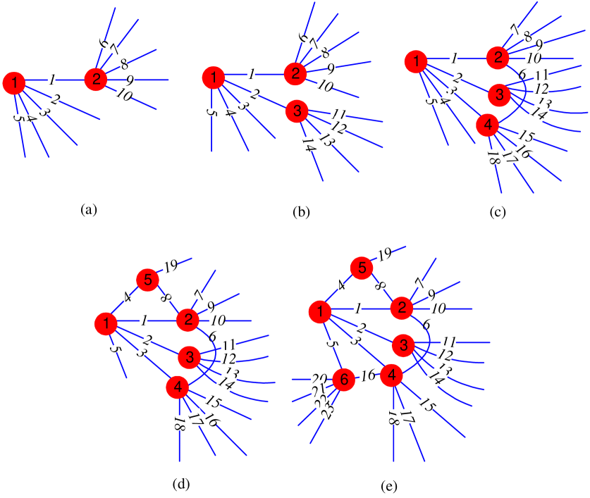
   Figure 12: The example of construction. The initialization is done in (a). Both or one of the two endnodes of links $1$-$23$ are determined.

   

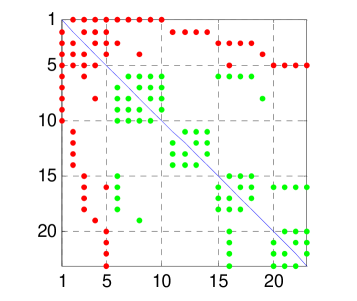
   Figure 13: The LAM of the constructed part (links $1$-$23$) of graph are computed. The green $1$-entries are determined by the red $1$-entries.

2. In the second step, we scan rows $6$ to $10$ of the LAM, since links $6$ to $10$ are incident to the same endnode. Let node $7$ be the endnode of link $7$, $21$ and $24$-$25$, and let node $8$ be the endnode of link $9$ and $20$, and let node $9$ be the endnode of link $10$, $14$ and $26$-$27$, as shown in Equation $\left(\ref{Eq_construction_example_2}\right)$ and Figure 14.

   $$\begin{array}[c]{c}\\ E=\end{array}\begin{array}[c]{c}\\ \left[\begin{array}[c]{c}\\ \\ \end{array}\right.\\ \\ \\ \\ \\ \\ \\ \end{array}\begin{tabular}[c]{cccccccccccccc}${\footnotesize 1}$&${\footnotesize 2}$&${\footnotesize 3}$&${\footnotesize 4}$&${\footnotesize 5}$&${\footnotesize 6}$&${\footnotesize 7}$&${\footnotesize 8}$&${\footnotesize 9}$&${\footnotesize 10}$&${\footnotesize 11}$&${\footnotesize 12}$&${\footnotesize 13}$&${\footnotesize 14}$\\ \hline\cr\vrule\lx@intercol\hfil$1$\hfil\lx@intercol &\vrule\lx@intercol\hfil$1$\hfil\lx@intercol &\vrule\lx@intercol\hfil$1$\hfil\lx@intercol &\vrule\lx@intercol\hfil$1$\hfil\lx@intercol &\vrule\lx@intercol\hfil$1$\hfil\lx@intercol &\vrule\lx@intercol\hfil$2$\hfil\lx@intercol &\vrule\lx@intercol\hfil$2$\hfil\lx@intercol &\vrule\lx@intercol\hfil$2$\hfil\lx@intercol &\vrule\lx@intercol\hfil$2$\hfil\lx@intercol &\vrule\lx@intercol\hfil$2$\hfil\lx@intercol &\vrule\lx@intercol\hfil$3$\hfil\lx@intercol &\vrule\lx@intercol\hfil$3$\hfil\lx@intercol &\vrule\lx@intercol\hfil$3$\hfil\lx@intercol &\vrule\lx@intercol\hfil$3$\hfil\lx@intercol\vrule\lx@intercol\\ \hline\cr\vrule\lx@intercol\hfil$2$\hfil\lx@intercol &\vrule\lx@intercol\hfil$3$\hfil\lx@intercol &\vrule\lx@intercol\hfil$4$\hfil\lx@intercol &\vrule\lx@intercol\hfil$5$\hfil\lx@intercol &\vrule\lx@intercol\hfil$6$\hfil\lx@intercol &\vrule\lx@intercol\hfil$4$\hfil\lx@intercol &\vrule\lx@intercol\hfil$7$\hfil\lx@intercol &\vrule\lx@intercol\hfil$5$\hfil\lx@intercol &\vrule\lx@intercol\hfil$8$\hfil\lx@intercol &\vrule\lx@intercol\hfil$9$\hfil\lx@intercol &\vrule\lx@intercol\hfil$0$\hfil\lx@intercol &\vrule\lx@intercol\hfil$0$\hfil\lx@intercol &\vrule\lx@intercol\hfil$0$\hfil\lx@intercol &\vrule\lx@intercol\hfil$9$\hfil\lx@intercol\vrule\lx@intercol\\ \hline\cr${\footnotesize 15}$&${\footnotesize 16}$&${\footnotesize 17}$&${\footnotesize 18}$&${\footnotesize 19}$&${\footnotesize 20}$&${\footnotesize 21}$&${\footnotesize 22}$&${\footnotesize 23}$&${\footnotesize 24}$&${\footnotesize 25}$&${\footnotesize 26}$&${\footnotesize 27}$&${\footnotesize 28}$\\ \hline\cr\vrule\lx@intercol\hfil$4$\hfil\lx@intercol &\vrule\lx@intercol\hfil$4$\hfil\lx@intercol &\vrule\lx@intercol\hfil$4$\hfil\lx@intercol &\vrule\lx@intercol\hfil$4$\hfil\lx@intercol &\vrule\lx@intercol\hfil$5$\hfil\lx@intercol &\vrule\lx@intercol\hfil$6$\hfil\lx@intercol &\vrule\lx@intercol\hfil$6$\hfil\lx@intercol &\vrule\lx@intercol\hfil$6$\hfil\lx@intercol &\vrule\lx@intercol\hfil$6$\hfil\lx@intercol &\vrule\lx@intercol\hfil$7$\hfil\lx@intercol &\vrule\lx@intercol\hfil$7$\hfil\lx@intercol &\vrule\lx@intercol\hfil$9$\hfil\lx@intercol &\vrule\lx@intercol\hfil$9$\hfil\lx@intercol &\vrule\lx@intercol\hfil$0$\hfil\lx@intercol\vrule\lx@intercol\\ \hline\cr\vrule\lx@intercol\hfil$0$\hfil\lx@intercol &\vrule\lx@intercol\hfil$6$\hfil\lx@intercol &\vrule\lx@intercol\hfil$0$\hfil\lx@intercol &\vrule\lx@intercol\hfil$0$\hfil\lx@intercol &\vrule\lx@intercol\hfil$0$\hfil\lx@intercol &\vrule\lx@intercol\hfil$8$\hfil\lx@intercol &\vrule\lx@intercol\hfil$7$\hfil\lx@intercol &\vrule\lx@intercol\hfil$0$\hfil\lx@intercol &\vrule\lx@intercol\hfil$0$\hfil\lx@intercol &\vrule\lx@intercol\hfil$0$\hfil\lx@intercol &\vrule\lx@intercol\hfil$0$\hfil\lx@intercol &\vrule\lx@intercol\hfil$0$\hfil\lx@intercol &\vrule\lx@intercol\hfil$0$\hfil\lx@intercol &\vrule\lx@intercol\hfil$0$\hfil\lx@intercol\vrule\lx@intercol\\ \hline\cr${\footnotesize 29}$&${\footnotesize\cdots}$&${\footnotesize 50}$&&&&&&&&&&&\\ \cline{1-3}\cr\vrule\lx@intercol\hfil$0$\hfil\lx@intercol &\vrule\lx@intercol\hfil$\cdots$\hfil\lx@intercol &\vrule\lx@intercol\hfil$0$\hfil\lx@intercol &\vrule\lx@intercol\hfil\hfil\lx@intercol &&&&&&&&&&\\ \cline{1-3}\cr\vrule\lx@intercol\hfil$0$\hfil\lx@intercol &\vrule\lx@intercol\hfil$\cdots$\hfil\lx@intercol &\vrule\lx@intercol\hfil$0$\hfil\lx@intercol &\vrule\lx@intercol\hfil\hfil\lx@intercol &&&&&&&&&&\\ \cline{1-3}\cr\end{tabular}\begin{array}[c]{c}\\ \\ \\ \\ \\ \\ \\ \left.\begin{array}[c]{c}\\ \\ \end{array}\right]\\ \end{array}$$ (8)

   

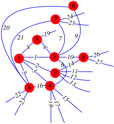
   Figure 14: The example of construction. Both or one of the two endnodes of links $1$-$27$ are determined.

   

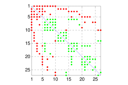
   Figure 15: The LAM of the constructed part (links $1$-$27)$ of graph are computed. The green $1$-entries are determined by the red $1$-entries.

3. Similarly, let node $10$ be the endnode of link $11$, $19$ and $28$-$30$, and let node $11$ be the endnode of link $12$, $18$ and $31$-$35$, and let node $12$ be the endnode of link $13$ and $36$, as shown in Equation $\left(\ref{Eq_construction_example_3}\right)$ and Figure 16 (a).

   $$\begin{array}[c]{c}\\ E=\end{array}\begin{array}[c]{c}\\ \left[\begin{array}[c]{c}\\ \\ \end{array}\right.\\ \\ \\ \\ \\ \\ \\ \end{array}\begin{tabular}[c]{cccccccccccccc}${\footnotesize 1}$&${\footnotesize 2}$&${\footnotesize 3}$&${\footnotesize 4}$&${\footnotesize 5}$&${\footnotesize 6}$&${\footnotesize 7}$&${\footnotesize 8}$&${\footnotesize 9}$&${\footnotesize 10}$&${\footnotesize 11}$&${\footnotesize 12}$&${\footnotesize 13}$&${\footnotesize 14}$\\ \hline\cr\vrule\lx@intercol\hfil$1$\hfil\lx@intercol &\vrule\lx@intercol\hfil$1$\hfil\lx@intercol &\vrule\lx@intercol\hfil$1$\hfil\lx@intercol &\vrule\lx@intercol\hfil$1$\hfil\lx@intercol &\vrule\lx@intercol\hfil$1$\hfil\lx@intercol &\vrule\lx@intercol\hfil$2$\hfil\lx@intercol &\vrule\lx@intercol\hfil$2$\hfil\lx@intercol &\vrule\lx@intercol\hfil$2$\hfil\lx@intercol &\vrule\lx@intercol\hfil$2$\hfil\lx@intercol &\vrule\lx@intercol\hfil$2$\hfil\lx@intercol &\vrule\lx@intercol\hfil$3$\hfil\lx@intercol &\vrule\lx@intercol\hfil$3$\hfil\lx@intercol &\vrule\lx@intercol\hfil$3$\hfil\lx@intercol &\vrule\lx@intercol\hfil$3$\hfil\lx@intercol\vrule\lx@intercol\\ \hline\cr\vrule\lx@intercol\hfil$2$\hfil\lx@intercol &\vrule\lx@intercol\hfil$3$\hfil\lx@intercol &\vrule\lx@intercol\hfil$4$\hfil\lx@intercol &\vrule\lx@intercol\hfil$5$\hfil\lx@intercol &\vrule\lx@intercol\hfil$6$\hfil\lx@intercol &\vrule\lx@intercol\hfil$4$\hfil\lx@intercol &\vrule\lx@intercol\hfil$7$\hfil\lx@intercol &\vrule\lx@intercol\hfil$5$\hfil\lx@intercol &\vrule\lx@intercol\hfil$8$\hfil\lx@intercol &\vrule\lx@intercol\hfil$9$\hfil\lx@intercol &\vrule\lx@intercol\hfil$10$\hfil\lx@intercol &\vrule\lx@intercol\hfil$11$\hfil\lx@intercol &\vrule\lx@intercol\hfil$12$\hfil\lx@intercol &\vrule\lx@intercol\hfil$9$\hfil\lx@intercol\vrule\lx@intercol\\ \hline\cr${\footnotesize 15}$&${\footnotesize 16}$&${\footnotesize 17}$&${\footnotesize 18}$&${\footnotesize 19}$&${\footnotesize 20}$&${\footnotesize 21}$&${\footnotesize 22}$&${\footnotesize 23}$&${\footnotesize 24}$&${\footnotesize 25}$&${\footnotesize 26}$&${\footnotesize 27}$&${\footnotesize 28}$\\ \hline\cr\vrule\lx@intercol\hfil$4$\hfil\lx@intercol &\vrule\lx@intercol\hfil$4$\hfil\lx@intercol &\vrule\lx@intercol\hfil$4$\hfil\lx@intercol &\vrule\lx@intercol\hfil$4$\hfil\lx@intercol &\vrule\lx@intercol\hfil$5$\hfil\lx@intercol &\vrule\lx@intercol\hfil$6$\hfil\lx@intercol &\vrule\lx@intercol\hfil$6$\hfil\lx@intercol &\vrule\lx@intercol\hfil$6$\hfil\lx@intercol &\vrule\lx@intercol\hfil$6$\hfil\lx@intercol &\vrule\lx@intercol\hfil$7$\hfil\lx@intercol &\vrule\lx@intercol\hfil$7$\hfil\lx@intercol &\vrule\lx@intercol\hfil$9$\hfil\lx@intercol &\vrule\lx@intercol\hfil$9$\hfil\lx@intercol &\vrule\lx@intercol\hfil$10$\hfil\lx@intercol\vrule\lx@intercol\\ \hline\cr\vrule\lx@intercol\hfil$0$\hfil\lx@intercol &\vrule\lx@intercol\hfil$6$\hfil\lx@intercol &\vrule\lx@intercol\hfil$0$\hfil\lx@intercol &\vrule\lx@intercol\hfil$11$\hfil\lx@intercol &\vrule\lx@intercol\hfil$10$\hfil\lx@intercol &\vrule\lx@intercol\hfil$8$\hfil\lx@intercol &\vrule\lx@intercol\hfil$7$\hfil\lx@intercol &\vrule\lx@intercol\hfil$0$\hfil\lx@intercol &\vrule\lx@intercol\hfil$0$\hfil\lx@intercol &\vrule\lx@intercol\hfil$0$\hfil\lx@intercol &\vrule\lx@intercol\hfil$0$\hfil\lx@intercol &\vrule\lx@intercol\hfil$0$\hfil\lx@intercol &\vrule\lx@intercol\hfil$0$\hfil\lx@intercol &\vrule\lx@intercol\hfil$0$\hfil\lx@intercol\vrule\lx@intercol\\ \hline\cr${\footnotesize 29}$&${\footnotesize 30}$&${\footnotesize 31}$&${\footnotesize 32}$&${\footnotesize 33}$&${\footnotesize 34}$&${\footnotesize 35}$&${\footnotesize 36}$&${\footnotesize 37}$&${\footnotesize\cdots}$&${\footnotesize 50}$&&&\\ \cline{1-11}\cr\vrule\lx@intercol\hfil$10$\hfil\lx@intercol &\vrule\lx@intercol\hfil$10$\hfil\lx@intercol &\vrule\lx@intercol\hfil$11$\hfil\lx@intercol &\vrule\lx@intercol\hfil$11$\hfil\lx@intercol &\vrule\lx@intercol\hfil$11$\hfil\lx@intercol &\vrule\lx@intercol\hfil$11$\hfil\lx@intercol &\vrule\lx@intercol\hfil$11$\hfil\lx@intercol &\vrule\lx@intercol\hfil$12$\hfil\lx@intercol &\vrule\lx@intercol\hfil$0$\hfil\lx@intercol &\vrule\lx@intercol\hfil$\cdots$\hfil\lx@intercol &\vrule\lx@intercol\hfil$0$\hfil\lx@intercol &\vrule\lx@intercol\hfil\hfil\lx@intercol &&\\ \cline{1-11}\cr\vrule\lx@intercol\hfil$0$\hfil\lx@intercol &\vrule\lx@intercol\hfil$0$\hfil\lx@intercol &\vrule\lx@intercol\hfil$0$\hfil\lx@intercol &\vrule\lx@intercol\hfil$0$\hfil\lx@intercol &\vrule\lx@intercol\hfil$0$\hfil\lx@intercol &\vrule\lx@intercol\hfil$0$\hfil\lx@intercol &\vrule\lx@intercol\hfil$0$\hfil\lx@intercol &\vrule\lx@intercol\hfil$0$\hfil\lx@intercol &\vrule\lx@intercol\hfil$0$\hfil\lx@intercol &\vrule\lx@intercol\hfil$\cdots$\hfil\lx@intercol &\vrule\lx@intercol\hfil$0$\hfil\lx@intercol &\vrule\lx@intercol\hfil\hfil\lx@intercol &&\\ \cline{1-11}\cr\end{tabular}\begin{array}[c]{c}\\ \\ \\ \\ \\ \\ \\ \left.\begin{array}[c]{c}\\ \\ \end{array}\right]\\ \end{array}$$ (9)

   

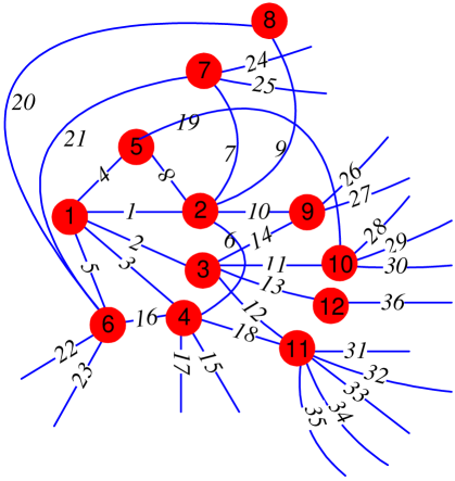
   Figure 16: The example of construction. Both or one of the two endnodes of links $1$-$36$ are determined.

   

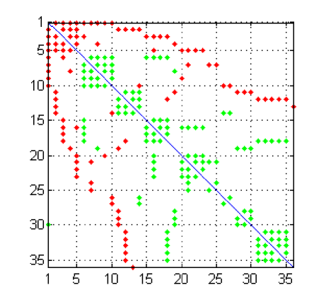
   Figure 17: The LAM of the constructed part (links $1$-$36)$ of graph are computed. The green $1$-entries are determined by the red $1$-entries.

4. Constructing in this way, the two endnodes of all the links are eventually determined, as shown in Equation $\left(\ref{Eq_construction_example_done}\right)$ and Figure 18 (a). The final structure of the matrix $E$ exhibits the link list of the original graph $G$ which consists of $30$ nodes and $50$ links. For example, link $36$ connects node $12$ and node $15$ in $G$. The matrix $E$ is readily transformed into the adjacency matrix of $G$.

   $$\begin{array}[c]{c}\\ E=\end{array}\begin{array}[c]{c}\\ \left[\begin{array}[c]{c}\\ \\ \end{array}\right.\\ \\ \\ \\ \\ \\ \\ \\ \\ \\ \end{array}\begin{tabular}[c]{cccccccccccccc}${\footnotesize 1}$&${\footnotesize 2}$&${\footnotesize 3}$&${\footnotesize 4}$&${\footnotesize 5}$&${\footnotesize 6}$&${\footnotesize 7}$&${\footnotesize 8}$&${\footnotesize 9}$&${\footnotesize 10}$&${\footnotesize 11}$&${\footnotesize 12}$&${\footnotesize 13}$&${\footnotesize 14}$\\ \hline\cr\vrule\lx@intercol\hfil$1$\hfil\lx@intercol &\vrule\lx@intercol\hfil$1$\hfil\lx@intercol &\vrule\lx@intercol\hfil$1$\hfil\lx@intercol &\vrule\lx@intercol\hfil$1$\hfil\lx@intercol &\vrule\lx@intercol\hfil$1$\hfil\lx@intercol &\vrule\lx@intercol\hfil$2$\hfil\lx@intercol &\vrule\lx@intercol\hfil$2$\hfil\lx@intercol &\vrule\lx@intercol\hfil$2$\hfil\lx@intercol &\vrule\lx@intercol\hfil$2$\hfil\lx@intercol &\vrule\lx@intercol\hfil$2$\hfil\lx@intercol &\vrule\lx@intercol\hfil$3$\hfil\lx@intercol &\vrule\lx@intercol\hfil$3$\hfil\lx@intercol &\vrule\lx@intercol\hfil$3$\hfil\lx@intercol &\vrule\lx@intercol\hfil$3$\hfil\lx@intercol\vrule\lx@intercol\\ \hline\cr\vrule\lx@intercol\hfil$2$\hfil\lx@intercol &\vrule\lx@intercol\hfil$3$\hfil\lx@intercol &\vrule\lx@intercol\hfil$4$\hfil\lx@intercol &\vrule\lx@intercol\hfil$5$\hfil\lx@intercol &\vrule\lx@intercol\hfil$6$\hfil\lx@intercol &\vrule\lx@intercol\hfil$4$\hfil\lx@intercol &\vrule\lx@intercol\hfil$7$\hfil\lx@intercol &\vrule\lx@intercol\hfil$5$\hfil\lx@intercol &\vrule\lx@intercol\hfil$8$\hfil\lx@intercol &\vrule\lx@intercol\hfil$9$\hfil\lx@intercol &\vrule\lx@intercol\hfil$10$\hfil\lx@intercol &\vrule\lx@intercol\hfil$11$\hfil\lx@intercol &\vrule\lx@intercol\hfil$12$\hfil\lx@intercol &\vrule\lx@intercol\hfil$9$\hfil\lx@intercol\vrule\lx@intercol\\ \hline\cr${\footnotesize 15}$&${\footnotesize 16}$&${\footnotesize 17}$&${\footnotesize 18}$&${\footnotesize 19}$&${\footnotesize 20}$&${\footnotesize 21}$&${\footnotesize 22}$&${\footnotesize 23}$&${\footnotesize 24}$&${\footnotesize 25}$&${\footnotesize 26}$&${\footnotesize 27}$&${\footnotesize 28}$\\ \hline\cr\vrule\lx@intercol\hfil$4$\hfil\lx@intercol &\vrule\lx@intercol\hfil$4$\hfil\lx@intercol &\vrule\lx@intercol\hfil$4$\hfil\lx@intercol &\vrule\lx@intercol\hfil$4$\hfil\lx@intercol &\vrule\lx@intercol\hfil$5$\hfil\lx@intercol &\vrule\lx@intercol\hfil$6$\hfil\lx@intercol &\vrule\lx@intercol\hfil$6$\hfil\lx@intercol &\vrule\lx@intercol\hfil$6$\hfil\lx@intercol &\vrule\lx@intercol\hfil$6$\hfil\lx@intercol &\vrule\lx@intercol\hfil$7$\hfil\lx@intercol &\vrule\lx@intercol\hfil$7$\hfil\lx@intercol &\vrule\lx@intercol\hfil$9$\hfil\lx@intercol &\vrule\lx@intercol\hfil$9$\hfil\lx@intercol &\vrule\lx@intercol\hfil$10$\hfil\lx@intercol\vrule\lx@intercol\\ \hline\cr\vrule\lx@intercol\hfil$13$\hfil\lx@intercol &\vrule\lx@intercol\hfil$6$\hfil\lx@intercol &\vrule\lx@intercol\hfil$14$\hfil\lx@intercol &\vrule\lx@intercol\hfil$11$\hfil\lx@intercol &\vrule\lx@intercol\hfil$10$\hfil\lx@intercol &\vrule\lx@intercol\hfil$8$\hfil\lx@intercol &\vrule\lx@intercol\hfil$7$\hfil\lx@intercol &\vrule\lx@intercol\hfil$15$\hfil\lx@intercol &\vrule\lx@intercol\hfil$16$\hfil\lx@intercol &\vrule\lx@intercol\hfil$13$\hfil\lx@intercol &\vrule\lx@intercol\hfil$17$\hfil\lx@intercol &\vrule\lx@intercol\hfil$18$\hfil\lx@intercol &\vrule\lx@intercol\hfil$19$\hfil\lx@intercol &\vrule\lx@intercol\hfil$19$\hfil\lx@intercol\vrule\lx@intercol\\ \hline\cr${\footnotesize 29}$&${\footnotesize 30}$&${\footnotesize 31}$&${\footnotesize 32}$&${\footnotesize 33}$&${\footnotesize 34}$&${\footnotesize 35}$&${\footnotesize 36}$&${\footnotesize 37}$&${\footnotesize 38}$&${\footnotesize 39}$&${\footnotesize 40}$&${\footnotesize 41}$&${\footnotesize 42}$\\ \hline\cr\vrule\lx@intercol\hfil$10$\hfil\lx@intercol &\vrule\lx@intercol\hfil$10$\hfil\lx@intercol &\vrule\lx@intercol\hfil$11$\hfil\lx@intercol &\vrule\lx@intercol\hfil$11$\hfil\lx@intercol &\vrule\lx@intercol\hfil$11$\hfil\lx@intercol &\vrule\lx@intercol\hfil$11$\hfil\lx@intercol &\vrule\lx@intercol\hfil$11$\hfil\lx@intercol &\vrule\lx@intercol\hfil$12$\hfil\lx@intercol &\vrule\lx@intercol\hfil$13$\hfil\lx@intercol &\vrule\lx@intercol\hfil$14$\hfil\lx@intercol &\vrule\lx@intercol\hfil$15$\hfil\lx@intercol &\vrule\lx@intercol\hfil$15$\hfil\lx@intercol &\vrule\lx@intercol\hfil$16$\hfil\lx@intercol &\vrule\lx@intercol\hfil$17$\hfil\lx@intercol\vrule\lx@intercol\\ \hline\cr\vrule\lx@intercol\hfil$20$\hfil\lx@intercol &\vrule\lx@intercol\hfil$21$\hfil\lx@intercol &\vrule\lx@intercol\hfil$22$\hfil\lx@intercol &\vrule\lx@intercol\hfil$23$\hfil\lx@intercol &\vrule\lx@intercol\hfil$24$\hfil\lx@intercol &\vrule\lx@intercol\hfil$21$\hfil\lx@intercol &\vrule\lx@intercol\hfil$16$\hfil\lx@intercol &\vrule\lx@intercol\hfil$25$\hfil\lx@intercol &\vrule\lx@intercol\hfil$23$\hfil\lx@intercol &\vrule\lx@intercol\hfil$26$\hfil\lx@intercol &\vrule\lx@intercol\hfil$17$\hfil\lx@intercol &\vrule\lx@intercol\hfil$26$\hfil\lx@intercol &\vrule\lx@intercol\hfil$24$\hfil\lx@intercol &\vrule\lx@intercol\hfil$24$\hfil\lx@intercol\vrule\lx@intercol\\ \hline\cr${\footnotesize 43}$&${\footnotesize 44}$&${\footnotesize 45}$&${\footnotesize 46}$&${\footnotesize 47}$&${\footnotesize 48}$&${\footnotesize 49}$&${\footnotesize 50}$&&&&&&\\ \cline{1-8}\cr\vrule\lx@intercol\hfil$17$\hfil\lx@intercol &\vrule\lx@intercol\hfil$17$\hfil\lx@intercol &\vrule\lx@intercol\hfil$18$\hfil\lx@intercol &\vrule\lx@intercol\hfil$23$\hfil\lx@intercol &\vrule\lx@intercol\hfil$23$\hfil\lx@intercol &\vrule\lx@intercol\hfil$23$\hfil\lx@intercol &\vrule\lx@intercol\hfil$27$\hfil\lx@intercol &\vrule\lx@intercol\hfil$27$\hfil\lx@intercol &\vrule\lx@intercol\hfil\hfil\lx@intercol &&&&&\\ \cline{1-8}\cr\vrule\lx@intercol\hfil$27$\hfil\lx@intercol &\vrule\lx@intercol\hfil$28$\hfil\lx@intercol &\vrule\lx@intercol\hfil$21$\hfil\lx@intercol &\vrule\lx@intercol\hfil$26$\hfil\lx@intercol &\vrule\lx@intercol\hfil$25$\hfil\lx@intercol &\vrule\lx@intercol\hfil$28$\hfil\lx@intercol &\vrule\lx@intercol\hfil$29$\hfil\lx@intercol &\vrule\lx@intercol\hfil$30$\hfil\lx@intercol &\vrule\lx@intercol\hfil\hfil\lx@intercol &&&&&\\ \cline{1-8}\cr\end{tabular}\begin{array}[c]{c}\\ \\ \\ \\ \\ \\ \\ \\ \\ \\ \left.\begin{array}[c]{c}\\ \\ \end{array}\right]\\ \end{array}$$ (10)

   

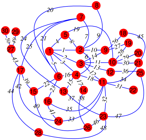
   Figure 18: The example of construction. The two endnodes of all links are determined.

   

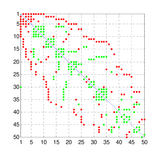
   Figure 19: The LAM of the constructed graph is computed. The green $1$-entries are determined by the red $1$-entries.

4.2.2 Initialization (The recognition of the endnodes of the first link and its neighboring links)

Algorithm 4 $E_{2\times L_{G}}\Leftarrow Initialization(C,s_{1},s_{2},s_{3})$

1:  if $s_{3}\geq 1$ then

2:     $E\Leftarrow\mathcal{E}$

3:  else if $s_{1}=1$ then

4:     $E\Leftarrow\mathcal{E}_{1}$

5:  else if $s_{1}=2$ then

6:     $E_{2\times L_{G}}\Leftarrow Initialization2(C,s_{2},s_{3})$

7:  else if $s_{1}=3$ then

8:     $E_{2\times L_{G}}\Leftarrow Initialization3(C,s_{2},s_{3})$

9:  else if $s_{1}\geq 4$ then

10:     $E_{2\times L_{G}}\Leftarrow Initialization4(C,s_{1},s_{2},s_{3})$

11:  end if

When $s_{3}\geq 1$, Theorem 6 implies that $s_{2}\geq 2$, $s_{1}\geq 3$ and links $2,3,\cdots,s_{3}+3$ are incident to the left endnode of link $1$ and links $s_{3}+4,\cdots,s_{1}+1$ are incident to the right endnode of link $1$. Therefore, line 1-2 of Algorithm 4 initialize $E$ by $\mathcal{E}$. The numbers above the matrix $\mathcal{E}$ in $\left(\ref{Eq_E5}\right)$ are the column numbers, which indicate the link numbers, and $\mathcal{E}$ has the following structure,

11⋯12⋯20⋯020⋯00⋯00⋯0​]\begin{array}[c]{c}\\ \mathcal{E}=\end{array}\begin{array}[c]{c}\\ \left[\begin{array}[c]{c}\\ \\ \end{array}\right.\end{array}\begin{tabular}[c]{cccccccccc}${\footnotesize 1}$&${\footnotesize 2}$&${\footnotesize\cdots}$&${\footnotesize s}_{3}{\footnotesize+3}$&${\footnotesize s}_{3}{\footnotesize+4}$&${\footnotesize\cdots}$&${\footnotesize s}_{1}{\footnotesize+1}$&${\footnotesize s}_{1}{\footnotesize+2}$&${\footnotesize\cdots}$&{\footnotesize$L_{G}$}\\ \hline\cr\vrule\lx@intercol\hfil$1$\hfil\lx@intercol &\vrule\lx@intercol\hfil$1$\hfil\lx@intercol &\vrule\lx@intercol\hfil$\cdots$\hfil\lx@intercol &\vrule\lx@intercol\hfil$1$\hfil\lx@intercol &\vrule\lx@intercol\hfil$2$\hfil\lx@intercol &\vrule\lx@intercol\hfil$\cdots$\hfil\lx@intercol &\vrule\lx@intercol\hfil$2$\hfil\lx@intercol &\vrule\lx@intercol\hfil$0$\hfil\lx@intercol &\vrule\lx@intercol\hfil$\cdots$\hfil\lx@intercol &\vrule\lx@intercol\hfil$0$\hfil\lx@intercol\vrule\lx@intercol\\ \hline\cr\vrule\lx@intercol\hfil$2$\hfil\lx@intercol &\vrule\lx@intercol\hfil$0$\hfil\lx@intercol &\vrule\lx@intercol\hfil$\cdots$\hfil\lx@intercol &\vrule\lx@intercol\hfil$0$\hfil\lx@intercol &\vrule\lx@intercol\hfil$0$\hfil\lx@intercol &\vrule\lx@intercol\hfil$\cdots$\hfil\lx@intercol &\vrule\lx@intercol\hfil$0$\hfil\lx@intercol &\vrule\lx@intercol\hfil$0$\hfil\lx@intercol &\vrule\lx@intercol\hfil$\cdots$\hfil\lx@intercol &\vrule\lx@intercol\hfil$0$\hfil\lx@intercol\vrule\lx@intercol\\ \hline\cr\end{tabular}\begin{array}[c]{c}\\ \left.\begin{array}[c]{c}\\ \\ \end{array}\right]\end{array}

12⋯+s33+s34⋯+s11+s12⋯LG (11)

When $s_{3}=0$, Theorem 6 cannot be used. However, the limited number of cases of $s_{3}=0$ enables us to accomplish the initialization with the detailed analysis in the Appendix A.

4.2.3 The recognition of the endnodes of the whole graph

Lines 1-2 of Algorithm 5 relabel the given LAM $C$ and determine the initial state. In the initial state, link $1$ is always incident to node $1$ and $2$. Some of the neighboring links of link $1$ are incident to node $1$, and the other neighboring links are incident to node $2$. The second endnodes of the neighboring links of link $1$ have not decided yet in the initial state.

Line 3 initiates the number of nodes $N_{G}$ to $2$. The two endnodes of link $1$ are already determined. Starting with link $2$ until link $L_{G}$ (line 4), the number of nodes $N_{G}$ increases by $1$ (line 6) if the second endnode of link $i$ is not determined (line 5). Let the second endnode of link $i$ be $N_{G}$ (line 7). When link $i$ is adjacent to link $j$, $j=i+1,\cdots,L_{G}$ (lines 8-9), let the first endnode of link $j$ be $N_{G}$ (line 11) if the first endnode of link $j$ is not determined (line 10). If the first endnode of link $j$ is determined but the second endnode is not determined and links $i$ and $j$ do not share the first endnode (line 12), let the second endnode of link $j$ be $N_{G}$ (line 13).

Algorithm 5 $E_{2\times L_{G}}\Leftarrow MARINLINGA(C)$

1:  $(C,s_{1},s_{2},s_{3})\Leftarrow MatrixRelabeling(C)$

2:  $E_{2\times L_{G}}\Leftarrow Initialization(C,s_{1},s_{2},s_{3})$

3:  $N\Leftarrow 2$

4:  for $i=2$ to $L_{G}$ do

5:     if $e_{2i}=0$ then

6:        $N\Leftarrow N+1$

7:        $e_{2i}\Leftarrow N$

8:        for $j=i+1$ to $L_{G}$ do

9:           if $c_{ij}=1$ then

10:              if $e_{1j}=0$ then

11:                 $e_{1j}\Leftarrow N$

12:              else if $e_{2j}=0$ and $e_{1i}\neq e_{1j}$ then

13:                 $e_{2j}\Leftarrow N$

14:              end if

15:           end if

16:        end for

17:     end if

18:  end for

4.3 Worst case complexity of MARINLINGA

Algorithm 1 has a complexity of $O\left(L_{G}\right)$. The complexity of Algorithm 3 can be computed as follows. Line 1 has a complexity of $O\left(L_{G}\right)$. In the worst case, the function of line 2, Algorithm 2 has a complexity of $O\left(L_{G}^{2}\right)$, if $m$ in line 15 of Algorithm 2 is proportional to $L_{G}$. The worst case complexity of lines 3-6 is also $O\left(L_{G}^{2}\right)$. Hence, lines 1-6 have a complexity of $O\left(L_{G}^{2}\right)$. Neglect $O\left(1\right)$ operations of lines 7-8. The times that lines 9-14 are executed is stored in $k$. If $k$ is proportional to $L_{G}$, $m$ in line 15 of Algorithm 2 must be bounded by a constant, then the complexity of line 11 is $O\left(L_{G}\right)$. If $k$ is bounded, the complexity of line 11 will be $O\left(L_{G}^{2}\right)$. Therefore, lines 9-14 have a worst case complexity of $O\left(L_{G}^{2}\right)$. Hence, the complexity of Algorithm 3 is $O\left(L_{G}^{2}\right)$.

Algorithm 6, 7 and 8 have a worst case complexity of $O\left(1\right)$, hence the complexity of Algorithm 4 is also $O\left(1\right)$. Lines 4-18 of the main Algorithm 5 have a worst case complexity of $O\left(L_{G}^{2}\right)$. In summary, the worst case complexity of the MARINLINGA is $O\left(L_{G}^{2}\right)$. Since the number of links of the original graph $G$ and the number of nodes of the line graph $l\left(G\right)$ are equal, $L_{G}=N_{l\left(G\right)}$, the worst case complexity of the MARINLINGA is written as $O\left(N_{l\left(G\right)}^{2}\right)$.

5 Comparison with Roussopoulos’s algorithm

We use the same input line graphs for both MARINLINGA and Roussopoulos’s algorithm. We start with line graphs constructed from Erdős-Rényi random graphs $G_{p}\left(N_{G}\right)$ [4]. We calculate the probability density function of the difference $\Delta T$ between the running time of Roussopoulos’s algorithm ($T_{\text{Roussopoulos}}$) and MARINLINGA ($T_{\text{MARINLINGA}}$)

$$\Delta T=T_{\text{Roussopoulos}}-T_{\text{MARINLINGA}}$$ (12)

We randomly create $1000$ different line graphs based on the class of Erdös-Rényi random graphs $G_{p}\left(N_{G}\right)$ for each number of nodes $N_{G}=\{10,20,30,50\}$ and link density $p=\{0.1,0.2,...,0.9\}$. The probability density functions of the time difference $f_{\Delta T}\left(x\right)$ for each class of line graphs of $G_{p}\left(N_{G}\right)$ are shown in Figure 20.

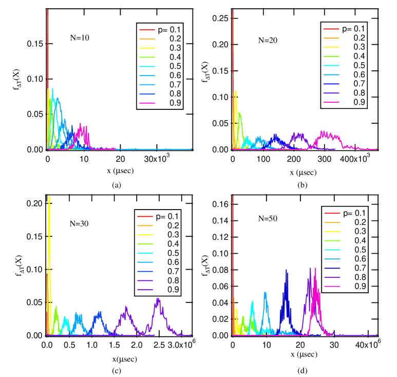
Figure 20: PDFs of the $\Delta T$ for $N=10,20,30$ and $50$ and $p=\{0.1,0.2,\ldots,0.9\}$

The values of the probability density function are nearly always positive which means in practice that MARINLINGA needs less time for the execution than Roussopoulos’s algorithm.

We calculate the expectation according to [13] and the experimental results for all of the mentioned cases $\Delta T_{i}$ for $i=1,2,\ldots,1000$.

$$E[\Delta T]=\sum k\text{ Pr}[\Delta T=k]=\frac{\sum_{i=1}^{1000}\Delta T_{i}}{1000}$$ (13)

The results in milliseconds are given in the Table 1.

	$N_{G}$	$10$	$20$	$30$	$50$
$\ \ p$
$.1$		$0.0462$	$0.7839$	$3.6660$	$42.8153$
$.2$		$0.1682$	$4.3012$	$26.1086$	$385.3208$
$.3$		$0.6281$	$11.9492$	$49.826$	$1582.5827$
$.4$		$1.3921$	$26.4580$	$209.3056$	$4802.8110$
$.5$		$2.4269$	$51.8393$	$422.8641$	$7060.6021$
$.6$		$3.5808$	$91.8258$	$719.6185$	$10978.1532$
$.7$		$4.9181$	$145.5864$	$1165.1978$	$15942.7395$
$.8$		$6.8952$	$217.2041$	$1768.9901$	$23393.5148$
$.9$		$9.2986$	$317.4966$	$2501.4799$	$24723.4739$

Table 1: Expectations of the time difference ($\mu$sec)

Additionally, we calculate the probability that MARINLINGA is slower than Roussopoulos’s algorithm: Pr$[\Delta T<0]$ for each $N_{G}$ and $p$. The simulation shows that Pr$[\Delta T<0]>0$ only for $N_{G}=10$ and $p\leq 0.2$, in which the graphs are mostly disconnected. When the graph is disconnected, MARINLINGA needs extra time to partition the graphs into connected components (see footnote 3). For $N_{G}=10$ and $p=0.1$, Pr$[\Delta T<0]=0.33$ and for $N_{G}=10$ and $p=0.2$, Pr$[\Delta T<0]=0.01$. For all the other cases

$$\text{Pr}[\Delta T<0]<0.001$$ (14)

which means that MARINLINGA is generally more efficient than Roussopoulos’s algorithm. The algorithm to find the maximal connected common subgraphs in graphs is frequently used in the Roussopoulos’s algorithm. This algorithm requires a high running time, because the problem of finding the maximal connected common subgraphs is $NP$-complete [16]. The dependence on this $NP$-complete algorithm is most significant weakness of Roussopoulos’s algorithm.

6 Conclusion

We have presented a new algorithm MARINLINGA for reverse line graph construction. By introducing the concept of LAM, we transformed the problem of reverse line graph construction into the problem of constructing a graph from the LAM. MARINLINGA consists of two sub-algorithms: the matrix relabeling algorithm and the construction algorithm. The matrix relabeling algorithm preprocesses the LAM into the special order by which we can determine the neighboring links of the first link and the endnodes of the first link incident to the neighboring links. The construction algorithm makes the first two nodes be the endnodes of the first link by default, and thereafter, determines the endnodes of the remaining links. MARINLINGA has a worst case complexity of $O(N_{l\left(G\right)}^{2})$, where $N_{l\left(G\right)}$ denotes the number of nodes of the line graph. We have demonstrated that MARINLINGA is more time-efficient compared to Roussopoulos’s algorithm for connected line graphs. The complexity of Roussopoulos’s algorithm mentioned in [12] is $O(N_{l\left(G\right)}+L_{l\left(G\right)})$, where $N_{l\left(G\right)}$ and $L_{l\left(G\right)}$ are number of nodes and links of the line graph. Since $L_{l\left(G\right)}=O\left(N_{l\left(G\right)}^{2}\right)$ in worst case, the complexity of Roussopoulos’s algorithm is also $O(N_{l\left(G\right)}^{2})$ in worst case. However, this analysis neglects the computational time of a sub-algorithm that determines the maximal connected common subgraph in each iteration. Finding a maximally connected common subgraph is an $NP$-complete problem [16], implying that Roussopoulos’s algorithm is, in fact, not polynomial in worst case.

Appendix A The initialization of the construction algorithm when $s_{3}=0$

Theorem 6 cannot be used when $s_{3}=0$. Since there exists limited number of cases of $s_{3}=0$, we can still accomplish the initialization.

A.1 When $s_{1}=1$

Link $1$ has only one right neighboring link: link $2$. Link $1$ does not have left neighboring links. The initial state of $E$ is $\mathcal{E}_{1}$. Lines 3-4 of Algorithm 4 initialize $E$ by $\mathcal{E}_{1}$.

$$\mathcal{E}_{1}=\left[\begin{tabular}[c]{ccccc}$1$&$2$&$0$&$\cdots$&$0$\\ $2$&$0$&$0$&$\cdots$&$0$\end{tabular}\ \ \ \ \ \right]$$ (15)

A.2 When $s_{1}=2$

There are different adjacency patterns. The submatrix of $C$ in Figure 21 (a) implies that, links $2$ and $3$ are adjacent to link $1$, and link $2$ is not not adjacent to link $3$. Links $2$ and $3$ must be incident to two different endnodes of link $1$. The pattern in Figure 21 (b) has two possible configurations $K_{3}$ and $K_{1,3}$. If $s_{1}=2$ and $s_{2}=0$, the initial state is $\mathcal{E}_{2,a}$, as shown in lines 1-2 of Algorithm 6. When $s_{1}=2$ and $s_{2}=1$, because the graph is connected, either $c_{2,4}=c_{3,4}=1$ or $c_{2,4}=0,c_{3,4}=1$ or $c_{2,4}=1,c_{3,4}=0$. If $c_{2,4}=c_{3,4}=1$, the initial state is $\mathcal{E}_{2,b.1}$, which is $K_{3}$, otherwise the initial state is $\mathcal{E}_{2,b.2}$, which is $K_{1,3}$, as shown in lines 8-12 of Algorithm 6.

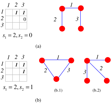
Figure 21: The adjacency patterns of link $1$ and its neighboring links when $s_{1}=2$. The graphs on the right are the possible configurations correspondingly.

$$\mathcal{E}_{2,a}=\left[\begin{tabular}[c]{cccccc}$1$&$1$&$2$&$0$&$\cdots$&$0$\\ $2$&$0$&$0$&$0$&$\cdots$&$0$\end{tabular}\ \ \ \ \ \right]$$ (16)

$$\mathcal{E}_{2,b.1}=\left[\begin{tabular}[c]{cccccc}$1$&$1$&$2$&$0$&$\cdots$&$0$\\ $2$&$0$&$0$&$0$&$\cdots$&$0$\end{tabular}\ \ \ \ \ \right],\mathcal{E}_{2,b.2}=\left[\begin{tabular}[c]{cccccc}$1$&$1$&$1$&$0$&$\cdots$&$0$\\ $2$&$0$&$0$&$0$&$\cdots$&$0$\end{tabular}\ \ \ \ \ \right]$$ (17)

Algorithm 6 $E_{2\times L_{G}}\Leftarrow Initialization2(C,s_{2})$

1:  if $s_{2}=0$ then

2:     $E\Leftarrow\mathcal{E}_{2,a}$

3:  else

4:     if $c_{2,4}=1$ and $c_{3,4}=1$ then

5:        $E\Leftarrow\mathcal{E}_{2,b.2}$

6:     else

7:        $E\Leftarrow\mathcal{E}_{2,b.1}$

8:     end if

9:  end if

A.3 When $s_{1}=3$

There are two recognizable adjacency patterns as described in Figure 22 (b), and (c). Taking pattern (c) as an example, links $1$, $2$ and $3$ are pairwise adjacent, then the configuration of them is $K_{3}$ or $K_{1,3}$, as shown in Figure 21 (b). Link $4$ is also adjacent to link $1$, but not adjacent to links $2$ and $3$, suggesting that the configuration of links $1$, $2$ and $3$ must be $K_{3}$, and link $4$ is incident to the other endnode of link $1$. Figure 22 (a) depicts the smallest forbidden link adjacency pattern in a LAM. The adjacency relation of links $1$, $2$ and $3$ is recognizable, and the configuration is a path on four nodes, as shown in Figure 21 (a). Link $4$ is adjacent to link $1$, then link $4$ must be also adjacent to links $2$ or $3$. Hence the pattern is forbidden. If $s_{1}=3$ and $s_{2}=0$, the initial state is $\mathcal{E}_{3,b}$ (lines 1-2 of Algorithm 7). If $s_{1}=3$, $s_{2}=1$ and $c_{3,4}=0$, the initial state is $\mathcal{E}_{3,c}$ (lines 3-5 of Algorithm 7). When $s_{1}=3$, $s_{2}=1$ and $c_{3,4}=1$, due to the connectivity of the concerned graph, either $c_{2,5}=c_{3,5}=c_{4,5}=1$ or $c_{2,5}=c_{3,5}=1,c_{4,5}=0$ or $c_{2,5}=c_{3,5}=0,c_{4,5}=1$ or $c_{2,5}=1,c_{3,5}=c_{4,5}=0$ or $c_{2,5}=0,c_{3,5}=c_{4,5}=1$. If $c_{2,5}\neq c_{3,5}$, the initial state is $\mathcal{E}_{3,d.2}$, else if $c_{2,5}=c_{3,5}\neq c_{4,5}$, the initial state is $\mathcal{E}_{3,d.1}$, else if $c_{2,5}=c_{3,5}=c_{4,5}=1$, we need to look further at the relation of $c_{2,6}$ and $c_{3,6}$: if $c_{2,6}\neq c_{3,6}$, the initial state is $\mathcal{E}_{3,d.2}$, else the initial state is $\mathcal{E}_{3,d.1}$ (lines 11-15 of Algorithm 7). If there are only 5 links in total and $c_{2,5}=c_{3,5}=c_{4,5}=1$, one can choose any of $\mathcal{E}_{3,d.1}$ and $\mathcal{E}_{3,d.2}$ as the initial state, and get isomorphic configurations. If $s_{1}=3$, $s_{2}=2$ and $s_{3}=0$, the same method is employed (lines 21-26 of Algorithm 7).

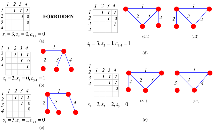
Figure 22: The adjacency patterns of link $1$ and its neighboring links when $s_{1}=3$. Pattern (a) is forbidden, and patterns (b), (c) and (f) correspond to only one configuration respectively. Patterns (d) and (e) both have two possible configurations.

$$\mathcal{E}_{3,b}=\left[\begin{array}[c]{ccccccc}1&1&2&2&0&\cdots&0\\ 2&0&0&0&0&\cdots&0\end{array}\right],\mathcal{E}_{3,c}=\left[\begin{array}[c]{ccccccc}1&1&1&2&0&\cdots&0\\ 2&0&0&0&0&\cdots&0\end{array}\right]$$ (18)

$$\mathcal{E}_{3,d.1}=\left[\begin{array}[c]{ccccccc}1&1&2&2&0&\cdots&0\\ 2&0&0&0&0&\cdots&0\end{array}\right],\mathcal{E}_{3,d.2}=\left[\begin{array}[c]{ccccccc}1&1&1&2&0&\cdots&0\\ 2&0&0&0&0&\cdots&0\end{array}\right]$$ (19)

$$\mathcal{E}_{3,e.1}=\left[\begin{array}[c]{ccccccc}1&1&2&1&0&\cdots&0\\ 2&0&0&0&0&\cdots&0\end{array}\right],\mathcal{E}_{3,e.2}=\left[\begin{array}[c]{ccccccc}1&1&1&2&0&\cdots&0\\ 2&0&0&0&0&\cdots&0\end{array}\right]$$ (20)

Algorithm 7 $E_{2\times L_{G}}\Leftarrow Initialization3(C,s_{2},s_{3})$

1:  if $s_{2}=0$ then

2:     $E\Leftarrow\mathcal{E}_{3,b}$

3:  else if $s_{2}=1$ and $c_{3,4}=0$ then

4:     $E\Leftarrow\mathcal{E}_{3,c}$

5:  else if $s_{2}=1$ and $c_{3,4}=1$ then

6:     if $c_{2,5}\neq c_{3,5}$ or ($c_{2,5}=c_{3,5}$ and $c_{2,5}=c_{4,5}$ and $L_{G}=5$) then

7:        $E\Leftarrow\mathcal{E}_{3,d.2}$

8:     else if $c_{2,5}=c_{3,5}$ and $c_{2,5}\neq c_{4,5}$ then

9:        $E\Leftarrow\mathcal{E}_{3,d.1}$

10:     else if $c_{2,5}=c_{3,5}$ and $c_{2,5}=c_{4,5}$ and $c_{2,6}=c_{3,6}$ then

11:        $E\Leftarrow\mathcal{E}_{3,d.1}$

12:     else if $c_{2,5}=c_{3,5}$ and $c_{2,5}=c_{4,5}$ and $c_{2,6}\neq c_{3,6}$ then

13:        $E\Leftarrow\mathcal{E}_{3,d.2}$

14:     end if

15:  else if $s_{2}=2$ and $s_{3}=0$ then

16:     if $c_{2,5}\neq c_{3,5}$ or ($c_{2,5}=c_{3,5}$ and $c_{2,5}=c_{4,5}$ and $L_{G}=5$) then

17:        $E\Leftarrow\mathcal{E}_{3,e.2}$

18:     else if $c_{2,5}=c_{3,5}$ and $c_{2,5}\neq c_{4,5}$ then

19:        $E\Leftarrow\mathcal{E}_{3,e.1}$

20:     else if $c_{2,5}=c_{3,5}$ and $c_{2,5}=c_{4,5}$ and $c_{2,6}=c_{3,6}$ then

21:        $E\Leftarrow\mathcal{E}_{3,e.1}$

22:     else if $c_{2,5}=c_{3,5}$ and $c_{2,5}=c_{4,5}$ and $c_{2,6}\neq c_{3,6}$ then

23:        $E\Leftarrow\mathcal{E}_{3,e.2}$

24:     end if

25:  end if

A.4 When $s_{1}\geq 4$

A.4.1 When $s_{2}\geq 3$

The configuration is unique. The initial state of $E$ is $\mathcal{E}_{4}$.

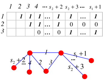
Figure 23: The adjacency pattern and the corresponding configuration when $s_{3}=0$, $s_{2}\geq 3$ and $s_{1}\geq 4$.

1121⋯12⋯20⋯02000⋯00⋯00⋯0​]\begin{array}[c]{c}\\ \mathcal{E}_{4}=\end{array}\begin{array}[c]{c}\\ \left[\begin{array}[c]{c}\\ \\ \end{array}\right.\end{array}\begin{tabular}[c]{cccccccccccc}${\footnotesize 1}$&${\footnotesize 2}$&${\footnotesize 3}$&${\footnotesize 4}$&${\footnotesize\cdots}$&${\footnotesize s}_{2}{\footnotesize+2}$&${\footnotesize s}_{2}{\footnotesize+3}$&${\footnotesize\cdots}$&${\footnotesize s}_{1}{\footnotesize+1}$&${\footnotesize s}_{1}{\footnotesize+2}$&${\footnotesize\cdots}$&{\footnotesize$L_{G}$}\\ \hline\cr\vrule\lx@intercol\hfil$1$\hfil\lx@intercol &\vrule\lx@intercol\hfil$1$\hfil\lx@intercol &\vrule\lx@intercol\hfil$2$\hfil\lx@intercol &\vrule\lx@intercol\hfil$1$\hfil\lx@intercol &\vrule\lx@intercol\hfil$\cdots$\hfil\lx@intercol &\vrule\lx@intercol\hfil$1$\hfil\lx@intercol &\vrule\lx@intercol\hfil$2$\hfil\lx@intercol &\vrule\lx@intercol\hfil$\cdots$\hfil\lx@intercol &\vrule\lx@intercol\hfil$2$\hfil\lx@intercol &\vrule\lx@intercol\hfil$0$\hfil\lx@intercol &\vrule\lx@intercol\hfil$\cdots$\hfil\lx@intercol &\vrule\lx@intercol\hfil$0$\hfil\lx@intercol\vrule\lx@intercol\\ \hline\cr\vrule\lx@intercol\hfil$2$\hfil\lx@intercol &\vrule\lx@intercol\hfil$0$\hfil\lx@intercol &\vrule\lx@intercol\hfil$0$\hfil\lx@intercol &\vrule\lx@intercol\hfil$0$\hfil\lx@intercol &\vrule\lx@intercol\hfil$\cdots$\hfil\lx@intercol &\vrule\lx@intercol\hfil$0$\hfil\lx@intercol &\vrule\lx@intercol\hfil$0$\hfil\lx@intercol &\vrule\lx@intercol\hfil$\cdots$\hfil\lx@intercol &\vrule\lx@intercol\hfil$0$\hfil\lx@intercol &\vrule\lx@intercol\hfil$0$\hfil\lx@intercol &\vrule\lx@intercol\hfil$\cdots$\hfil\lx@intercol &\vrule\lx@intercol\hfil$0$\hfil\lx@intercol\vrule\lx@intercol\\ \hline\cr\end{tabular}\begin{array}[c]{c}\\ \left.\begin{array}[c]{c}\\ \\ \end{array}\right]\end{array}

1234⋯+s22+s23⋯+s11+s12⋯LG (21)

A.4.2 When $s_{2}\leq 2$

There are $13$ forbidden patterns, as shown in Figure 24, where the links with labels larger than $5$ are not displayed. The pattern in Figure 22 (a) is forbidden, hence the $4$ patterns in Figure 24 (a.1) are also forbidden, where x can be $1$ or $0$. The pattern of links $1-4$ in Figure 24 (a.2-3) is the same as the pattern in Figure 22 (b), which has a specific configuration. In Figure 24 (a.2), link $5$ is adjacent to link $1$ but not $2$, then link $5$ must be adjacent to link $3$, which is not true, hence the $2$ patterns in Figure 24 (a.2) are forbidden. In Figure 24 (a.3), link $5$ is adjacent to link $1$ and $3$, then link $5$ must be adjacent to link $4$, which is not true, hence the pattern in Figure 24 (a.3) is also forbidden. Similarly, based on the patterns in Figure 22, we can conclude that patterns in Figure 24 (b.1), (b.3), (c.1), (c.3), (d.1) and (d.4) are also forbidden. Based on the values of entries $s_{2}$, $c_{3,4}$, $c_{3,5}$ and $c_{4,5}$, Algorithm 8 decides the initial state of $E$.

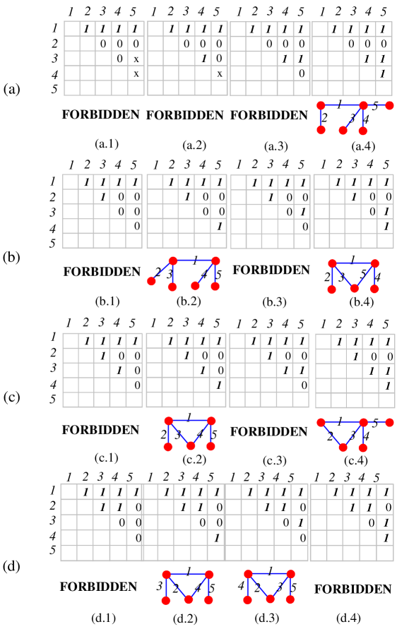
Figure 24: The adjacency patterns of link $1$ and its neighboring links when $s_{1}=4$. There are $16$ forbidden patterns. The other $12$ possible patterns correspond to only one configuration respectively. The entry x can be $1$ or $0$.

11222⋯20⋯020000⋯00⋯0​]\mathcal{E}_{4,a.4}=\mathcal{E}_{4,c.4}=\begin{array}[c]{c}\\ \left[\begin{array}[c]{c}\\ \\ \end{array}\right.\end{array}\begin{tabular}[c]{cccccccccc}${\footnotesize 1}$&${\footnotesize 2}$&${\footnotesize 3}$&${\footnotesize 4}$&${\footnotesize 5}$&${\footnotesize\cdots}$&${\footnotesize s}_{1}{\footnotesize+1}$&${\footnotesize s}_{1}{\footnotesize+2}$&${\footnotesize\cdots}$&{\footnotesize$L_{G}$}\\ \hline\cr\vrule\lx@intercol\hfil$1$\hfil\lx@intercol &\vrule\lx@intercol\hfil$1$\hfil\lx@intercol &\vrule\lx@intercol\hfil$2$\hfil\lx@intercol &\vrule\lx@intercol\hfil$2$\hfil\lx@intercol &\vrule\lx@intercol\hfil$2$\hfil\lx@intercol &\vrule\lx@intercol\hfil$\cdots$\hfil\lx@intercol &\vrule\lx@intercol\hfil$2$\hfil\lx@intercol &\vrule\lx@intercol\hfil$0$\hfil\lx@intercol &\vrule\lx@intercol\hfil$\cdots$\hfil\lx@intercol &\vrule\lx@intercol\hfil$0$\hfil\lx@intercol\vrule\lx@intercol\\ \hline\cr\vrule\lx@intercol\hfil$2$\hfil\lx@intercol &\vrule\lx@intercol\hfil$0$\hfil\lx@intercol &\vrule\lx@intercol\hfil$0$\hfil\lx@intercol &\vrule\lx@intercol\hfil$0$\hfil\lx@intercol &\vrule\lx@intercol\hfil$0$\hfil\lx@intercol &\vrule\lx@intercol\hfil$\cdots$\hfil\lx@intercol &\vrule\lx@intercol\hfil$0$\hfil\lx@intercol &\vrule\lx@intercol\hfil$0$\hfil\lx@intercol &\vrule\lx@intercol\hfil$\cdots$\hfil\lx@intercol &\vrule\lx@intercol\hfil$0$\hfil\lx@intercol\vrule\lx@intercol\\ \hline\cr\end{tabular}\begin{array}[c]{c}\\ \left.\begin{array}[c]{c}\\ \\ \end{array}\right]\end{array}

12345⋯+s11+s12⋯LG (22)

11122⋯20⋯020000⋯00⋯0​]\mathcal{E}_{4,b.2}=\mathcal{E}_{4,b.4}=\mathcal{E}_{4,c.2}=\mathcal{E}_{4,d.2}=\begin{array}[c]{c}\\ \left[\begin{array}[c]{c}\\ \\ \end{array}\right.\end{array}\begin{tabular}[c]{cccccccccc}${\footnotesize 1}$&${\footnotesize 2}$&${\footnotesize 3}$&${\footnotesize 4}$&${\footnotesize 5}$&${\footnotesize\cdots}$&${\footnotesize s}_{1}{\footnotesize+1}$&${\footnotesize s}_{1}{\footnotesize+2}$&${\footnotesize\cdots}$&{\footnotesize$L_{G}$}\\ \hline\cr\vrule\lx@intercol\hfil$1$\hfil\lx@intercol &\vrule\lx@intercol\hfil$1$\hfil\lx@intercol &\vrule\lx@intercol\hfil$1$\hfil\lx@intercol &\vrule\lx@intercol\hfil$2$\hfil\lx@intercol &\vrule\lx@intercol\hfil$2$\hfil\lx@intercol &\vrule\lx@intercol\hfil$\cdots$\hfil\lx@intercol &\vrule\lx@intercol\hfil$2$\hfil\lx@intercol &\vrule\lx@intercol\hfil$0$\hfil\lx@intercol &\vrule\lx@intercol\hfil$\cdots$\hfil\lx@intercol &\vrule\lx@intercol\hfil$0$\hfil\lx@intercol\vrule\lx@intercol\\ \hline\cr\vrule\lx@intercol\hfil$2$\hfil\lx@intercol &\vrule\lx@intercol\hfil$0$\hfil\lx@intercol &\vrule\lx@intercol\hfil$0$\hfil\lx@intercol &\vrule\lx@intercol\hfil$0$\hfil\lx@intercol &\vrule\lx@intercol\hfil$0$\hfil\lx@intercol &\vrule\lx@intercol\hfil$\cdots$\hfil\lx@intercol &\vrule\lx@intercol\hfil$0$\hfil\lx@intercol &\vrule\lx@intercol\hfil$0$\hfil\lx@intercol &\vrule\lx@intercol\hfil$\cdots$\hfil\lx@intercol &\vrule\lx@intercol\hfil$0$\hfil\lx@intercol\vrule\lx@intercol\\ \hline\cr\end{tabular}\begin{array}[c]{c}\\ \left.\begin{array}[c]{c}\\ \\ \end{array}\right]\end{array}

12345⋯+s11+s12⋯LG (23)

11212⋯20⋯020000⋯00⋯0​]\mathcal{E}_{4,d.3}=\begin{array}[c]{c}\\ \left[\begin{array}[c]{c}\\ \\ \end{array}\right.\end{array}\begin{tabular}[c]{cccccccccc}${\footnotesize 1}$&${\footnotesize 2}$&${\footnotesize 3}$&${\footnotesize 4}$&${\footnotesize 5}$&${\footnotesize\cdots}$&${\footnotesize s}_{1}{\footnotesize+1}$&${\footnotesize s}_{1}{\footnotesize+2}$&${\footnotesize\cdots}$&{\footnotesize$L_{G}$}\\ \hline\cr\vrule\lx@intercol\hfil$1$\hfil\lx@intercol &\vrule\lx@intercol\hfil$1$\hfil\lx@intercol &\vrule\lx@intercol\hfil$2$\hfil\lx@intercol &\vrule\lx@intercol\hfil$1$\hfil\lx@intercol &\vrule\lx@intercol\hfil$2$\hfil\lx@intercol &\vrule\lx@intercol\hfil$\cdots$\hfil\lx@intercol &\vrule\lx@intercol\hfil$2$\hfil\lx@intercol &\vrule\lx@intercol\hfil$0$\hfil\lx@intercol &\vrule\lx@intercol\hfil$\cdots$\hfil\lx@intercol &\vrule\lx@intercol\hfil$0$\hfil\lx@intercol\vrule\lx@intercol\\ \hline\cr\vrule\lx@intercol\hfil$2$\hfil\lx@intercol &\vrule\lx@intercol\hfil$0$\hfil\lx@intercol &\vrule\lx@intercol\hfil$0$\hfil\lx@intercol &\vrule\lx@intercol\hfil$0$\hfil\lx@intercol &\vrule\lx@intercol\hfil$0$\hfil\lx@intercol &\vrule\lx@intercol\hfil$\cdots$\hfil\lx@intercol &\vrule\lx@intercol\hfil$0$\hfil\lx@intercol &\vrule\lx@intercol\hfil$0$\hfil\lx@intercol &\vrule\lx@intercol\hfil$\cdots$\hfil\lx@intercol &\vrule\lx@intercol\hfil$0$\hfil\lx@intercol\vrule\lx@intercol\\ \hline\cr\end{tabular}\begin{array}[c]{c}\\ \left.\begin{array}[c]{c}\\ \\ \end{array}\right]\end{array}

12345⋯+s11+s12⋯LG (24)

Algorithm 8 $E_{2\times L_{G}}\Leftarrow Initialization4(C,s_{1},s_{2},s_{3})$

1:  if $s_{2}\geq 3$ then

2:     $E\Leftarrow\mathcal{E}_{4}$

3:  else if $s_{2}=0$ or ($s_{2}=1$ and $c_{3,4}=1$ and $c_{3,5}=1$ and $c_{4,5}=1$) then

4:     $E\Leftarrow\mathcal{E}_{4,a.4}$

5:  else if $s_{2}=1$ and $c_{3,4}=0$ and $c_{4,5}=1$ then

6:     $E\Leftarrow\mathcal{E}_{4,b.2}$

7:  else if $s_{2}=1$ and $c_{3,4}=1$ and $c_{3,5}=0$ and $c_{4,5}=1$ then

8:     $E\Leftarrow\mathcal{E}_{4,c.2}$

9:  else if $s_{2}=2$ and $c_{4,5}=1$ then

10:     $E\Leftarrow\mathcal{E}_{4,d.2}$

11:  else if $s_{2}=2$ and $c_{4,5}=0$ then

12:     $E\Leftarrow\mathcal{E}_{4,d.3}$

13:  end if

References

- [1] Yong-Yeol Ahn, James P. Bagrow, and Sune Lehmann. Link communities reveal multiscale complexity in networks. Nature, 466(7307):761–764, June 2010.
- [2] L. W. Beineke. Characterizations of derived graphs. Journal of Combinatorial Theory, 9:129–135, 1970.
- [3] D. G. Degiorgi and K. Simon. A dynamic algorithm for line graph recognition. In WG ’95: Proceedings of the 21st International Workshop on Graph-Theoretic Concepts in Computer Science, pages 37–48, London, UK, 1995. Springer-Verlag.
- [4] P. Erdős and A. Rényi. On random graphs. Publicationes Mathematicae Debrecen, 6:290–297, 1959.
- [5] T. Evans and R. Lambiotte. Overlapping communities, link partitions and line graphs. Proceedings of the European Conference on Complex Systems ’09, 2009.
- [6] T. S. Evans and R. Lambiotte. Line graphs, link partitions, and overlapping communities. Phys. Rev. E, 80(1):016105, Jul 2009.
- [7] F. Harary. Graph Theory. Addison-Wesley, Reading, 1969.
- [8] P. G. H. Lehot. An optimal algorithm to detect a line graph and output its root graph. J. ACM, 21(4):569–575, 1974.
- [9] D. Liu and P. Van Mieghem. On random line graphs. Working in process.
- [10] A. Manka-Krason, A. Mwijage, and K. Kulakowski. Clustering in random line graphs. Computer Physics Communications, 181(1):118–121, 2010.
- [11] J. Naor and M. B. Novick. An efficient reconstruction of a graph from its line graph in parallel. J. Algorithms, 11(1):132–143, 1990.
- [12] N. D. Roussopoulos. A max {m,n} algorithm for determining the graph h from its line graph g. Information Processing Letters, 2(4):108–112, 1973.
- [13] P. Van Mieghem. Performance Analysis of Communications Networks and Systems. Cambridge University Press, 2006.
- [14] P. Van Mieghem. Graph Spectra for Complex Networks. Cambridge University Press, 2010.
- [15] A. van Rooij and H. Wilf. The interchange graphs of a finite graph. Acta Math. Acad. Sci. Hungar., 16:263–269, 1965.
- [16] Vismara. Finding Maximum Common Connected Subgraphs Using Clique Detection or Constraint Satisfaction Algorithms. In MCO’08: Modelling, Computation and Optimization in Information Systems and Management Sciences, Communications in Computer and Information Science, pages 364–374. Springer Berlin Heidelberg, 09 2008.
- [17] H. Whitney. Congruent graphs and the connectivity of graphs. American Journal of Mathematics, 54:150–168, 1932.
- [18] J. C. Wierman, D. P. Naor, and J. Smalletz. Incorporating variability into an approximation formula for bond percolation thresholds of planar periodic lattices. Phys. Rev. E, 75(1):011114, Jan 2007.