Pulse propagation in decorated random chains

Abstract

We study pulse propagation in one-dimensional chains of spherical granules decorated with small randomly-sized granules placed between bigger monodisperse ones. Such “designer chains” are of interest in efforts to control the behavior of the pulse so as to optimize its propagation or attentuation, depending on the desired application. We show that a recently proposed effective description of simple decorated chains can be extended to predict pulse properties in chains decorated with small granules of randomly chosen radii. Furthermore, we also show that the binary collision approximation can again be used to provide analytic results for this system.

I Introduction

The study of pulse propagation in granular media has become a field of intense research interest. This is partly due to the fundamental importance of understanding the associated nonlinear dynamics and partly due to its direct application to our day-to-day lives. Any system in which interactions among its discrete constituents are solely described by their macroscopic geometrical shapes and elasticity properties rather than by their microscopic (atomic or molecular) nature can be classified as granular system. Among granular systems, a class that draws special attention is that of so-called dry granular systems. A defining property of these systems is that the intergranule interaction potentials are always positive i.e., they are purely mutually repulsive. Furthermore, they are only nonzero as long as the two bodies are in physical contact. This peculiarity, together with the spatially discrete nature of granular systems, gives rise to a host of interesting phenomena. Depending on parameter values, granular systems can express liquid-like, solid-like (glasses), or gas-like properties KadanoffRMP99 ; SilbertPRL05 .

It is well known that an initial kinetic energy impulse imparted to an edge granule of a chain in the absence of precompression can result in solitary waves propagating through the medium nesterenko ; nesterenko-1 . In the recent past, pulse propagation in one-dimensional (1D) chains of granules has been studied extensively both theoretically and experimentally nesterenko-book ; application ; alexandremono ; alexandre ; jean ; wangPRE07 ; rosasPRL07 ; rosasPRE08 ; sen-review ; costePRE97 ; nesterenkoJP94 ; sokolowEPL07 ; wu02 ; robertPRE05 ; sokolowAPL05 ; senPHYA01 ; meloPRE06 ; jobGM07 ; senJAP09 . These studies are in part inspired by a number of practical applications, e.g., in the design of shock absorbers DarioPRL06 ; HongPRL05 , sound scramblers VitaliPRL05 ; DaraioPRE05 and actuating devices KhatriSIMP08 .

Structural variations along a granular chain can significantly influence pulse propagation through the system. These structural variations (or polydispersity) are frequently introduced in a regular fashion such as in tapered chains, in which the size and/or mass of successive granules systematically decreases or increases. A detailed study of these effects has been carried out numerically senJAP09 ; wangPRE07 ; sen-review ; robertPRL06 ; wu02 ; robertPRE05 ; sokolowAPL05 ; senPHYA01 . In our own recent work PRE09 we introduced a binary collision model to derive fairly simple analytic results to describe pulse propagation in various 1D tapered chains. We showed that most of the essential properties that characterize pulse propagation in tapered chains can be extremely accurately described in these systems using the binary collision model.

Recently we turned our attention to more complex chain configurations, specifically, to decorated chains, that is, to chains in which large and small granules alternate in some regular fashion. These chains can not be studied directly using any binary collision model, and the reason is quite obvious: as a pulse propagates, the small granules rattle back and forth between their larger neighbors and thus at least three granules rather than two are involved in elementary collision events. However, we introduced an effective description PRE2 whereby we represented decorated chains by associated undecorated ones. We tested this methodology on a variety of simple and tapered decorated chains and showed that the effective undecorated chains reproduced the behavior of pulse propagation in the original decorated ones in all cases provided the small decorating granules were sufficiently small (see below). This effective representation can then be treated analytically using the binary collision approximation. The resulting analytic expressions allow us to explore regimes in which numerical algorithms may be unstable, and even regimes where the pulse amplitude becomes so weak as to be close to the numerical noise.

All the studies described above have dealt with chains with regular configurations, be they monodisperse or tapered, simple or decorated. Here we introduce a new element, namely randomness. It is interesting to study the effects of randomness because (1) most granular systems in nature are not regular, and (2) randomness might be used as a control element in manipulating pulse propagation properties in designed systems. It therefore becomes important to understand effects of randomness on pulse propagation. Except for recent work by Fraternali et al. DaraioMAMS09 , we are not aware of any other work on pulse propagation in random granular chains. In this work we develop an understanding of some effects of randomness on pulse propagation. For this purpose, we extend our previous work on decorated chains PRE2 to incorporate effects of randomness.

Our randomly decorated chain is constructed from a monodisperse array of large granules separated pairwise by smaller granules whose size is randomly picked from a pre-assigned distribution. For our effective description PRE2 to be valid, the radius of the smaller granules must be no larger than $\sim 40\%$ of the larger granules. This places a restriction on the upper cutoff of the size distribution of smaller granules. We show that a randomly decorated chain can then be mapped onto an effective undecorated chain with random masses and random interactions. We find that for all properties studied herein, the behavior of our effective chain (obtained from the numerical solution of the equations of motion for this chain) is in remarkable agreement with the behavior of the original decorated chain (obtained from the numerical solution of its equations of motion). In particular, we focus on three properties of the pulse. First, we compute the pulse amplitude and its variation along the chain. Second, we determine the average speed of the pulse along the chain. Third, we calculate the distribution of the times that the pulse takes to reach the end of the chain.

We then go on to test our binary collision approximation applied to the effective chain. We find that whereas the approximation does not reproduce the pulse amplitude well (for reasons that we understand and for which we suggest a possible remedy), the other two properties are extremely well predicted analytically by the model. This provides a powerful tool to avoid costly numerical simulations.

In Sec. II we introduce the granular chain model in terms of rescaled (dimensionless) variables. In Sec. III we introduce decorated chains and present our effective description in terms of undecorated chains with renormalized interactions and masses. The analysis here is a generalization of the work of Ref. PRE2 to accommodate the random variation (within limits) of the radii of the smaller granules. In this section we also exhibit the analytic results obtained by applying the binary collision approximation to the effective chain. Comparisons with numerical results are presented in Sec. IV. In Sec. V we provide a summarizing closure.

II The model

We consider chains of granules all made of the same material of density $\rho$. When neighboring granules collide, they repel each other according to the power law potential

$$V=\frac{a}{n}r_{k}^{\prime}|y_{k}-y_{k+1}|^{n}.$$ (1)

Here $y_{k}$ is the displacement of granule $k$ from its position at the beginning of the collision, and $a$ is a constant determined by Young’s modulus and Poisson’s ratio landau ; hertz . The exponent $n$ is $5/2$ for spheres (Hertz potential), which we use throughout this paper in our explicit calculations hertz . We have defined

$$r_{k}^{\prime}=\left(\frac{2R_{k}^{\prime}R_{k+1}^{\prime}}{R_{k}^{\prime}+R_{k+1}^{\prime}}\right)^{1/2},$$ (2)

where $R_{k}^{\prime}$ is the principal radius of curvature of the surface of granule $k$ at the point of contact. When the granules do not overlap, the potential is zero. The equation of motion for the $k$th granule is

$$M_{k}\frac{d^{2}y_{k}}{d{\tau}^{2}} = {a}{r}_{k-1}^{\prime}(y_{k-1}-y_{k})^{n-1}\theta(y_{k-1}-y_{k})$$ (3)

$$- {a}{r}_{k}^{\prime}(y_{k}-y_{k+1})^{n-1}\theta(y_{k}-y_{k+1}),$$

where $M_{k}=(4/3)\pi\rho(R_{k}^{\prime})^{3}$. The Heaviside function $\theta(y)$ ensures that the elastic interaction between grains is only nonzero if they are in contact. Initially the granules are placed along a line so that they just touch their neighbors in their equilibrium positions (no precompression), and all but the leftmost particle are at rest. The initial velocity of the leftmost particle ($k=1$) is $V_{1}$ (the impulse). We define the dimensionless quantity

$$\alpha\equiv\left[\frac{M_{1}V_{1}^{2}}{a\left(R_{1}^{\prime}\right)^{n+1/2}}\right]$$ (4)

and the rescaled quantities $x_{k}$, $t$, $m_{k}$, and $R_{k}$ via the relations

$$y_{k}=R_{1}^{\prime}\alpha^{1/n}x_{k}, \tau=\frac{R_{1}^{\prime}}{V_{1}}\alpha^{1/n}t,$$

$$R_{k}^{\prime}=R_{1}^{\prime}R_{k}, M_{k}=M_{1}m_{k}.$$ (5)

Equation (3) can then be rewritten as

$$m_{k}\ddot{x}_{k} = r_{k-1}(x_{k-1}-x_{k})^{n-1}\theta(x_{k-1}-x_{k})$$ (6)

$$-r_{k}(x_{k}-x_{k+1})^{n-1}\theta(x_{k}-x_{k+1}),$$

where a dot denotes a derivative with respect to $t$, and

$$r_{k}=\left(\frac{2R_{k}R_{k+1}}{R_{k}+R_{k+1}}\right)^{1/2}.$$ (7)

The rescaled initial velocity is unity, i.e., $v_{1}(t=0)=1$. The velocity of the $k$-th granule in unscaled variables is simply $V_{1}$ times its velocity in the scaled variables.

III Theoretical results: effective chain and binary collision approximation

III.1 Effective chain

We consider a decorated chain with a small granule inserted between each pair of large granules. The end granules are large, and the large granules are monodisperse. The sizes of the small granules are random. In order to obtain an effective description for the pulse dynamics in the decorated chain, we follow the scheme presented in Ref. PRE2 . In that work we showed that the effective description could be constructed using the outcome of a detailed analysis of a chain of five granules. This five-granule chain provides the elements of all the granules in the actual long chain: large granules in the interior of the chain, small granules in the interior of the chain, and large granules at the ends of the chain.

Consider, then, a chain of five granules labeled from $k-2$ to $k+2$ in unit steps, granules $k-1$ and $k+1$ being the small granules. The radius of the large granules is $R_{1}\equiv R=1$ in rescaled variables, and those of the small granules is $R_{k}=R_{k}^{\prime}/R_{1}^{\prime}$. The dynamics of this chain of granules is governed by the set of equations,

$$m_{k-2}\ddot{x}_{k-2} = -r_{k-2}(x_{k-2}-x_{k-1})^{n-1}\theta(x_{k-2}-x_{k-1})$$

$$m_{i}\ddot{x}_{i} = r_{i-1}(x_{i-1}-x_{i})^{n-1}\theta(x_{i-1}-x_{i})$$

$$- r_{i}(x_{i}-x_{i+1})^{n-1}\theta(x_{i}-x_{i+1}),~{}~{}i=k,k\pm 1,$$

$$m_{k+2}\ddot{x}_{k+2} = r_{k+1}(x_{k+1}-x_{k+2})^{n-1}\theta(x_{k+1}-x_{k+2}).$$ (8)

Since all the large granules are of the same size, it follows that $m_{k-2}=m_{k+1}=m_{k+2}=m$ ($=1$ in the rescaled units), and we have $r_{k-1}=r_{k-2}$ and $r_{k}=r_{k+1}$, which just says that for a given small granule the left and right sides are geometrically identical. Following Ref. PRE2 , this chain can be mapped onto an effective chain of three large granules which we call “left” ($l$), “right” ($r$), and “between” ($b$), with renormalized masses $\mu_{l}$, $\mu_{r}$ and $\mu_{b}$ given by

$$\mu_{l} = m+\frac{1}{2}m_{k-1},~{}~{}~{}\mu_{r}=m+\frac{1}{2}m_{k+1}$$

$$\mu_{b} = m+\frac{1}{2}(m_{k-1}+m_{k+1}).$$ (9)

The effective interaction between two neighboring large granules in this three-grain configuration is

$$V_{eff}(k,k+1)=\frac{r_{k}}{n2^{n-1}}(x_{k}-x_{k+1})^{n},$$ (10)

where

$$r_{k}=\sqrt{\frac{2R_{k}}{1+R_{k}}}.$$ (11)

Now we return to the actual long chain, which is made of $N$ large granules and $N-1$ small ones. Our effective chain then has $N$ effective granules where each of the two edge granules corresponds to either the “left” or the “right” effective granule described above, and the rest of the granules in the chain are described according to the “between” granule prescription. We emphasize that since the size $R_{k}$ of the smaller granules is a random variable, the renormalized masses, Eq. (III.1), and the effective interactions, Eq. (10), in the effective chain are also random variables. This completes the mapping onto an effective chain. This mapping in turn allows us to implement the binary collision approximation, which we do next.

III.2 Binary collision approximation

Using the binary collision approximation, in our previous studies we successfully calculated the time that it takes the pulse to reach the end of the chain. For this purpose we first calculate the time spent by the pulse at each granule. If we assume that in the effective chain the pulse propagates through a series of successive binary collisions, the time taken by the pulse to go from the $k$th granule to the $(k+1)$st granule in the chain is given by

$$T_{k,k+1}=A(n)\left[\frac{{\cal M}_{k,k+1}}{r_{k}}\right]^{1/n}v_{k}^{\frac{2}{n}-1},$$ (12)

where

$$A(n)=\sqrt{\pi}\frac{\Gamma(1+1/n)}{\Gamma(1/2+1/n)}(2^{n-2}n)^{1/n},$$ (13)

and ${\cal M}_{k,k+1}=\mu_{k}\mu_{k+1}/(\mu_{k}+\mu_{k+1})$ is the reduced mass for the pair of granules $k$ and $(k+1)$ PRE2 . The velocity amplitude $v_{k}$ in Eq. (12) is

$$v_{k}=\prod_{n=1}^{k-1}\frac{2{\cal M}_{n,n+1}}{\mu_{n+1}}.$$ (14)

The time taken by the pulse to reach the end of the chain is therefore

$$t_{N} = \sum_{k=1}^{N-1}T_{k,k+1}$$ (15)

$$= A(n)\sum_{k=1}^{N-1}\left[\frac{{\cal M}_{k,k+1}}{r_{k}}\right]^{1/n}v_{k}^{\frac{2}{n}-1}.$$

Suppose now that the small granules are chosen randomly from a given distribution, i.e., their sizes and consequently their masses are random variables. This means that each $k$-dependent term on the right hand side of Eq. (12) is a random variable. To help us manage these contributions, we implement two further approximations for Eq. (15). First, since the radius of the small granules is restricted to be no larger than 40% of that of the large granules, $R_{k}\leq 0.4$, we neglect the correction of order $R_{k}^{3}$ to the masses of the (large) granules in the effective chain. All granules in the effective chain then have equal (fixed) masses equal to that of the large masses in the original chain [see Eq.(III.1)]. Thus $v_{k}=1$ and ${\cal M}_{k,k+1}=m/2$. Equation (15) then reduces to

$$t_{N}=A(n)\left(\frac{m}{2}\right)^{1/n}\sum_{k=1}^{N-1}\left(\frac{1+R_{k}}{2R_{k}}\right)^{\frac{1}{2n}}.$$ (16)

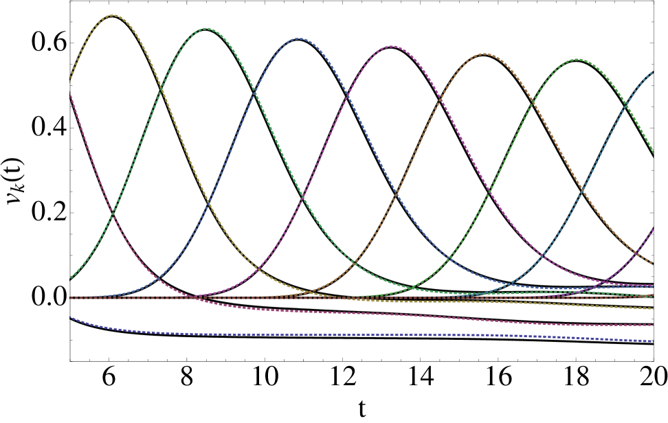
Figure 1: (Color online) Averaged velocity profile of the larger granules with $N=11$. Results from the effective scheme are shown as black continuous curves.

Secondly, we assume that $R_{k}$ is sufficiently small to neglect it in the numerator of the above expression, which is consistent with the requirement for the validity of the effective description in the first place. We thus approximate Eq. (16) as

$$t_{N}\approx A(n)\left(\frac{m}{2}\right)^{1/n}\sum_{k=1}^{N-1}\left(2R_{k}\right)^{-\frac{1}{2n}}$$ (17)

(this assumption might be questionable when $R_{k}$ is as large as $0.4$, but the results shown later support the applicability of this approximation).

Although all the formulas given above are valid for any distribution function subject to the stated restrictions, for concreteness we implement a uniform distribution of small radii over the interval $[\alpha,\beta]$. It can easily be shown that each term $X_{k}=(R_{k})^{-1/2n}$ on the right hand side of Eq. (17) is then distributed over the range $[\beta^{-\frac{1}{2n}},\alpha^{-\frac{1}{2n}}]$ according to

$$P(X_{k})=\frac{2n}{\beta-\alpha}X_{k}^{-(2n+1)}.$$ (18)

Since this distribution has finite first and second moments, as $N\to\infty$ it follows from the central limit theorem that the sum over the independent random variables $X_{k}$ tends to a Gaussian distribution. The mean and the variance of the Gaussian are obtained from the mean ($\kappa$) and the variance ($\sigma^{2}$) of the underlying distribution. Thus for large $N$, $t_{N}$ is distributed around the mean $N\kappa$ with a variance given by $N\sigma^{2}$. It is straightforward to see that the average time $\langle t_{N}\rangle$ then varies linearly with $N$, $\langle t_{N}\rangle\approx S(N-1)$, and the slope of the line is given by

$$S=\frac{2nA(n)}{2n-1}\left(\frac{m}{2^{3/2}}\right)^{1/n}\left(\frac{\beta^{1-1/(2n)}-\alpha^{1-1/(2n)}}{\beta-\alpha}\right).$$ (19)

We stress that Eq. (17) and consequently (19) are valid when the effect of randomness is negligible on the masses of the large granules and is only important in modifying the effective interactions between them. Note that within the binary collision approximation these expressions can be used not only to calculate the time that the pulse takes to arrive at the end of the chain but to arrive at any specified granule of the chain.

In the next section we shall compare these results with the numerical solution of the exact equations and also with the numerical solution of the equations for the effective chain.

IV Comparison with numerical results

To restate our scenario, we consider a chain of $N$ identical large granules, each pair of which is separated by a small granule. In all our chains the first and the last granules are of the large variety. The radii of the $(N-1)$ small granules (or masses) are randomly selected from a uniform distribution in the range $[\alpha,\beta]$. For all of our numerical results we choose $\alpha=0.01$ and $\beta=0.4$. The value of $\beta=0.4$ (and no larger) is dictated by the validity of the effective description. Note that for $\beta=0.4$, the mass of granules in the effective chain (Eq. III.1) can randomly increase by up to $\sim 6\%$ of the mass of the large granules in the original chain. The density of all granules is the same. The equation of motion for each granule is given by Eq. (6). We solve the set of $2N-1$ coupled equations numerically for a large number of realizations ($\sim 30000$) of the radii of the small granules. In this section we compare these solutions with the corresponding results for the effective chain, and also with those obtained from the binary collision approximation to the effective chain.

In Fig. 1 we show the velocity amplitude profile of the bigger granules averaged over all realizations. We observe that a well-behaved (average) pulse of time-varying amplitude and width propagates through the random chain. In the same figure we show the results obtained from the effective description, where the granular masses and their interactions are given by Eqs. (III.1) and (10), respectively. The two results are almost identical, thus showing that a description in terms of the effective chain is valid even in the presence of randomness.

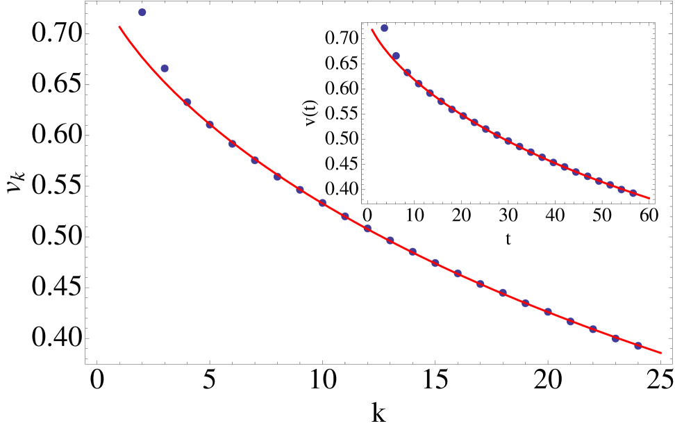
Figure 2: (Color online) Decay in the average pulse velocity amplitude as a function of the (larger) granular number $k$ in the effective chain with $N=26$. The continuous curve represents the stretched exponential decay $v_{k}=a\exp(-bk^{c})$ with $a=0.756,b=0.067$ and $c=0.714$. Inset: stretched exponential decay in the pulse velocity amplitude as a function of time $t$.

In Fig. 2 we show the change in the pulse amplitude as it passes from one large granule to the next along the chain. The results are indistinguishable between the original decorated chain and the effective chain. The amplitude follows a stretched exponential decay $v_{k}=a\exp(-bk^{c})$ with fitted parameter values $a=0.756$, $b=0.067$, and $c=0.714$. The inset in the figure shows the stretched exponential decay in the pulse amplitude as a function of time, $v(t)=a^{\prime}\exp(-b^{\prime}t^{c^{\prime}})$ with $a^{\prime}=0.744$, $b^{\prime}=0.035$, and $c^{\prime}=0.714$. Note that $c=c^{\prime}$, indicating that time $t$ and granule number $k$ are linearly related, i.e., $t\propto k$.

The variation of $t$ with $k$ in the original chain or in the effective chain (they are again indistinguishable) is shown in Fig. 3 for $N=26$. The linear relation between $k$ and $t$ was obtained in our earlier work on pulse propagation in monodisperse granular chains alexandremono ; alexandre . The slope of this linear variation in time as obtained from the fit to the numerical data is $\approx 2.402$. This is within $2\%$ of the value $S=2.348$ obtained from the binary colision approximation, Eq. (19). Thus the effective chain as well as the binary collision approximation to it yield excellent results in agreement with those of the original chain for the variation of the pulse propagation time as a function of granule number.

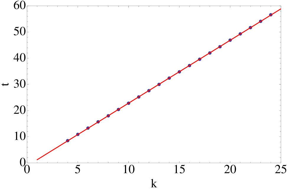
Figure 3: (Color online) Average pulse propagation time as a function of $k$ for $N=26$ for the effective chain. The straight line is the fit $t=2.402k-1.181$.

The effective chain captures the behavior of the original chain extremely well for all the properties considered above. Indeed, the behavior of the two is essentially indistinguishable. We now go on to assess the validity of the binary collision approximation for the effective chain. Above we showed that the average pulse propagation time as a function of granule number is captured very accurately by the approximation. Next we focus on the distribution of times that the pulse takes to reach the end of the chain. Because of the randomness in the chain, this time is distributed around a mean. We compute the distribution of this time by solving the exact dynamical equations of motion for the decorated chain over a large number of realizations ($\sim$ 30000) of the distribution of smaller granules. The theoretical prediction for this time obtained from the binary collision model is given by Eq. (15). In Fig. 4 we show comparisons between the theory (filled circles) and the numerical results (empty circles) for various lengths of the chain. In showing the comparison in Fig. 4, we have adjusted the peak position of the distribution obtained from the theory, which gives slightly higher values of the peak position. This shift arises from the small error in the prediction of the pulse velocity when using the binary collision approximation. In calculating the distribution of arrival times, this small error is accumulated over all the terms in the sum, that is, it is in effect multiplied by $N$, the length of the chain. However, we note that the amplitude and the shape of the distribution are very well reproduced by the theory.

For a short chain ($N=6,11$) the distribution of arrival times of the pulse at the edge of the chain is quite asymmetric. This asymmetry decreases as the length of the chain is increased, and for $N=26$ the distribution is approaching a Gaussian. This is the result of the central limit theorem. Remember that in Eq. (15) we are adding random terms. However these terms are not independent (each term contains information about the random size/mass of all the previous granules through $v_{k}$), and therefore the sum is more complicated than one involving independent random variables. In any case, since for large $N$ the sum assumes a Gaussian-like form, the correlation between different terms in Eq. (15) is presumably small or highly localized (falling off quickly with increasing $k$).

$\begin{array}[]{cc}\rotatebox{0.0}{\scalebox{0.2}{\includegraphics{Figure4ul.eps}}}&\rotatebox{0.0}{\scalebox{0.2}{\includegraphics{Figure4ur.eps}}}\\ \rotatebox{0.0}{\scalebox{0.2}{\includegraphics{Figure4lr.eps}}}&\rotatebox{0.0}{\scalebox{0.2}{\includegraphics{Figure4ll.eps}}}\end{array}$

Figure 4: The distribution of arrival times of the pulse to granule $k=2N-3$. This is the large granule before the last large granule at the end of a chain of $2N-1$ granules. Here $N=6,11,16,26$ starting from the left upper panel and changing in the clockwise direction. Filled circles: theory; empty circles: numerics.

In order to quantify the difference between the computed distribution functions in Fig. 4 and the standard normal distribution, we have performed the Kolomogorov-Smirnov KS statistical test on the data obtained numerically and used to generate the distribution shown in the figure. For this purpose, we first collect the data $\{X_{n}=x_{1},x_{2},\cdots x_{n}\}$ computed from the numerical solution in increasing order $x_{1}<x_{2}<\cdots x_{n}$. Then the mean $\mu_{n}$ and the standard deviation $\sigma_{n}$ are computed as

$$\mu(n) = \frac{1}{n}\sum_{i=1}^{n}x_{i}$$

$$\sigma(n) = \sqrt{\frac{1}{n-1}\sum_{i=1}^{n}(x_{i}-\mu)^{2}}.$$ (20)

A new data set $z_{n}=(X_{n}-\mu(n))/\sigma(n)$ is then generated. The Kolmogorov-Smirnov test involves computing the statistics of the absolute difference (non-directional hypothesis) between the cumulative frequency distribution $F_{z}(n)$ of $z_{n}$ and that of the standard normal distribution $F_{0}$, i.e., $d=|F_{z}(n)-F_{0}|$ KS . Acceptance of the null hypothesis that the distribution is Gaussian within a given level of confidence requires that $d$ be appropriately small. Consistent with the progression seen in Fig. 4, we find a steady decrease in the value of $d$ as $N$ increases, that is, our distribution approaches a Gaussian.

Finally, we turn to the velocity amplitude, which while extremely well reproduced in the effective undecorated chain is not captured well by the binary collision approximation. It is easy to see the source of the problem. Recall that Eq. (19) is valid only when the masses of the granules in the effective chain are assumed to all be equal and only the interactions between them are affected by the randomness of the sizes of the smaller granules. The agreement between the theory, Eq. (19), and the numerics indicates that these assumptions are valid when calculating pulse travel times. However, the velocity obtained from the model as posed in Eq. (14) is independent of $k$ (and only very weakly dependent on $k$ if the direct $\lesssim 6\%$ effect of the randomness of the masses is not neglected) and does not follow the behavior observed in the numerical solution of the exact equations, Fig. 2. The problem lies in the fact that the velocity $v_{k}$ obtained from the binary model depends only on the mass ratio of two colliding granules. However, the random interactions can introduce unavoidable three (or more) granule scenarios. For example, if the interaction between a granule $1$ and a granule $2$ is weak but that between $2$ and $3$ is strong, then a collision between $1$ and $2$ will inevitably involve granule $3$. A remedy might be to include this effect through a further renormalization of the masses resulting from the random interactions. This will be explored in future work.

V conclusions

We have studied pulse propagation in 1D granular chains decorated with small granules of random radii inserted between each pair of large granules all of the same size. This study has proceded in two steps.

Firstly, we used the effective scheme introduced in Ref. PRE2 to obtain an equivalent undecorated random chain, and showed that this effective description works remarkably well for all properties tested, so well that the numerical results obtained from the original chain and from the effective chain are essentially indistinguishable. Since the effective chain is only half as long as the original chain, this represents a considerable savings in computational effort.

Secondly, using the binary collision approximation on the effective chain, we have obtained analytic expressions for the velocity amplitude of the pulse and the time that the pulse takes to reach the $k$th granule (pulse speed $dk/dt$) along the chain. By construction, the analytic results obtained using the binary collision approximation neglect the effects of the randomness of the small granules on the masses of the large granules in the effective chain. The randomness appears only in the interactions between granules. It is thus not surprising that the velocity amplitude of the pulse obtained from the binary model does not predict the correct behavior as seen in numerical results, since this amplitude is determined by the masses of colliding granules and is therefore affected by the randomness of these masses. In the previous section we have suggested a possible remedy to this issue. On the other hand, the pulse speed and the distribution of the times taken by the pulse to reach the $k$th granule are very well reproduced by the theory. This is because the time of pulse propagation depends on the interactions, being shorter (longer) for stronger (weaker) interactions. Our theory incorporates this dependence very accurately, cf. Eq. (15).

As was noted in Ref. PRE2 , the effective description works well as long as the size of the small granule remains less than $\sim 40\%$ of the bigger granule. This places a restriction on the size/mass distribution of the smaller granules. Here, for simplicity, we have considered a uniform distribution of the smaller granules. However, the validity of the effective description and of the binary-collision approximation will remain valid for arbitrary distributions as long as the size restriction on the small granules is satisfied. In future work we plan to generalize our effective chain description (and the associated binary collision approximation) to other chain configurations, with the eventual goal of understanding pulse propagation in chains of arbitrary granular configurations.

References

- (1) L. P. Kadanoff, Rev. Mod. Phys. 71, 435 (1999).
- (2) L. E. Silbert, Phys. Rev. Lett. 94, 098002 (2005).
- (3) V. F. Nesterenko, J. Appl. Mech. tech. Phys. 24, 733 (1983).
- (4) A. N. Lazaridi and V. F. Nesterenko, J. Appl. Mech. Technol. Phys. 26, 405 (1985).
- (5) V. F. Nesterenko, Dynamics of Heterogeneous Materials, Springer, New York (2001)
- (6) S. Job, F. Melo, A. Sokolow, and S.Sen, Phys. Rev. Lett. 94, 178002 (2005).
- (7) A. Rosas and K. Lindenberg, Phys. Rev. E 68 041304 (2003).
- (8) A. Rosas and K. Lindenberg, Phys. Rev. E 69 037601 (2004).
- (9) E. J. Hinch and S. Saint-Jean, Proc. R. Soc. London, Ser. A 455, 3201 (1999).
- (10) P. J. Wang, J. H. Xia, Y. D. Li, and C. S. Liu, Phys. Rev. E 76, 041305 (2007).
- (11) S. Sen, Phys. Rep. 462, 21 (2008).
- (12) D. T. Wu, Physica A, 315, 194 (2002).
- (13) R. Doney and S. Sen, Phys. Rev. E, 72, 041304 (2005).
- (14) A. Sokolow, J. M. M. Pfannes, R. L. Doney, M. Nakagawa, J. H. Agui and S. Sen, Appl. Phys. Lett. 87, 154104 (2005).
- (15) S. Sen, F.S. Manciu and M. Manciu, Physica A 299, 551 (2001).
- (16) R. L. Doney, J. H. Agui and S. Sen, J. Appl. Phys. 106 064905 (2009).
- (17) A. Rosas, A. H. Romero, V. F. Nesterenko and K. Lindenberg, Phys. Rev. Lett. 98, 164301 (2007).
- (18) A. Rosas, A. H. Romero, V. F. Nesterenko and K. Lindenberg, Phys. Rev. E 78, 051303 (2008).
- (19) C. Coste, E. Falcon and S. Fauve, Phys. Rev. E 56, 6104 (1994).
- (20) V. F. Nesterenko, J. Phys. IV 4(C8), 729 (1994).
- (21) A. Sokolow, E. G. Bittle and S. Sen, Europhys. Lett. 77, 24002 (2007).
- (22) F. Melo, S. Job, F. Santibanez and F. Tapia, Phys. Rev. E 73 041305 (2006).
- (23) S. Job, F. Melo, A. Sokolow and S. Sen, Granular Matter 10, 13 (2007).
- (24) C. Daraio, V. F. Nesterenko, E. B. Herbold and S. Jin, Phys. Rev. Lett. 96, 058002 (2006).
- (25) J. Hong, Phys. Rev. Lett. 94, 108001 (2005).
- (26) V. F. Nesterenko, C. Daraio, E. B. Herbold and S. Jin, Phys. Rev. Lett. 95, 158702 (2005).
- (27) C. Daraio, V. F. Nesterenko, E. B. Herbold and S. Jin, Phys. Rev. E 72, 016603 (2005).
- (28) D. Khatri, C. Daraio and P. Rizzo, SPIE 6934, 69340U (2008).
- (29) R. Doney and S. Sen, Phys. Rev. Lett. 97, 155502 (2006).
- (30) U. Harbola, A. Rosas, M. Esposito and K. Lindenberg, Phys. Rev. E 80, 031303 (2009).
- (31) U. Harbola, A. Rosas, A. Romero, M. Esposito and K. Lindenberg, Phys. Rev. E, 80 051302 (2009).
- (32) F. Fraternali, M. A. Porter and C. Daraio, Mech. Adv. Mat. Structure 16, 8 (2009).
- (33) L. D. Landau and E. M. Lifshitz, Theory of Elasticity (Addison-Wesley, Massachusetts, 1959).
- (34) H. Hertz, . Reine Angew. Math. 92, 156 (1881).
- (35) D. J. Sheskin, Handbook of Parametric and Nonparametric Statistical Procedures, 2nd Edition, Chapman Hall/CRC, Florida (2000).