Anisotropies in the Diffuse Gamma-Ray Background from Dark Matter with Fermi LAT: a closer look
Abstract
We perform a detailed study of the sensitivity to the anisotropies related to Dark Matter (DM) annihilation in the Isotropic Gamma-Ray Background (IGRB) as measured by the Fermi Large Area Telescope (Fermi-LAT). For the first time, we take into account the effects of the Galactic foregrounds and use a realistic representation of the Fermi-LAT. We implement an analysis pipeline which simulates Fermi-LAT data sets starting from model maps of the Galactic foregrounds, the Fermi resolved point sources, the extra-galactic diffuse emission and the signal from DM annihilation. The effects of the detector are taken into account by convolving the model maps with the Fermi-LAT instrumental response. We then use the angular power spectrum to characterize the anisotropy properties of the simulated data and to study the sensitivity to DM. We consider DM anisotropies of extra-galactic origin and of Galactic origin (which can be generated through annihilation in the Milky Way sub-structures) as opposed to a background of anisotropies generated by sources of astrophysical origin, blazars for example. We find that with statistics from 5 years of observation Fermi is sensitive to a DM contribution at the level of 1%-10% of the measured IGRB depending on the DM mass and annihilation mode. In terms of the thermally averaged cross section , this corresponds to cm3s-1, i.e. slightly above the typical expectations for a thermal relic, for low values of the DM mass GeV. The anisotropy method for DM searches has a sensitivity comparable to the usual methods based only on the energy spectrum and thus constitutes an independent and complementary piece of information in the DM puzzle.
1 Introduction
Combined studies of the cosmic microwave background radiation, supernova cosmology and large Galaxy redshift surveys provide nowadays compelling evidence of the existence of non-baryonic Dark Matter (DM) [Komatsu at al. 2008, Tegmark et al. 2006]. Consistency with the observed structure of the Universe, especially at large (above galactic) scales favors Cold Dark Matter (CDM), i.e. the particles constituting the cosmologically required dark matter have to be moving non-relativistically. This property is always fulfilled by particles of mass in the GeV to TeV region that interact with the weak interaction strength, i.e. weakly interacting massive particles (WIMPs). WIMPs can annihilate or decay to detectable standard model particles, in particular gamma-rays, giving rise to the possibility of “indirect detection” [Bertone et al. 2004, Jungman et al. 1995, Bergstrom 2000, Baltz et al. 2008]. A standard approach is to look for spectral signatures in the energy spectrum of gamma-rays from celestial objects, either targeting the continuum spectrum produced by decay of secondary pions or the more feeble signature of a line due to DM annihilating directly into photons.
Another possible experimental signature is given by differences in the spatial distribution of gamma-ray signals induced by DM as compared to conventional astrophysical sources. In particular, the small scale fluctuations in an otherwise isotropic gamma-ray background (IGRB) might be different in the case of annihilating DM, since its flux scales as the squared density. After the pioneering study of Ando and Komatsu [Ando & Komatsu 2006] , followed by two other more detailed works [Ando et al. 2006, Ando et al. 2007], the issue of DM annihilation and anisotropies in the isotropic gamma background has raised increasing interest. In connection to the extra-galactic gamma-ray background, anisotropy has been further studied in [Cuoco et al. 2006, Cuoco et al. 2007, Cuoco 2008] while predictions from the Millenium II simulation have recently been described in Zavala et al. (2009). It has also been realized that Galactic substructures can produce an almost isotropic gamma background with similar fluctuation properties as the extragalactic background and with promising chances of detection [Siegal-Gaskins 2008, Ando 2009, Siegal-Gaskins and Pavlidou 2009, Hensley et al. 2009]; see also [Pieri et al. 2007, Pieri et al. 2009]). Other works have investigated the anisotropy pattern resulting from both the Galactic and extragalactic contribution [Fornasa et al. 2009, Hooper & Serpico 2007, Ibarra et al. 2010] or from the the DM annihilation around intermediate mass black holes [Taoso et al. 2009]. Anisotropies from DM annihilation appearing in the radio sky have been investigated in [Zhang and Sigl 2008]. Finally,– apart from the power spectrum – an interesting approach is to investigate the probability distribution of the fluctuations in order to detect possible departures from Gaussianity (or, rather, from Poisson statistics, in the common situation of low number of counts), thereby providing another handle on the separation of conventional astrophysical and DM contribution [Lee et al. 2008, Dodelson et al. 2009]. Anisotropy properties of astrophysical processes other than DM contributing to the isotropic gamma background include resolved point sources [Ando et al. 2006], galaxy clusters and shocks [Miniati et al. 2007, Keshet et al. 2003] and emission from normal galaxies [Ando & Pavlidou 2009].
The Fermi Large Area Telescope (Fermi-LAT), which was launched June 11, 2008, is the most suitable tool for these kind of studies due to its large field of view ( 2.4 sr), energy coverage from 100 MeV to 300 GeV [Atwood et al. 2009] and very good angular resolution. We will thus focus in the following on the prospect to detect DM anisotropies with Fermi-LAT.
All of the above studies assume either that the impact of Galactic foregrounds on the DM induced anisotropies is negligible or that the Galactic foregrounds can be cleaned at a suitable level to allow DM anisotropies studies. Further, the effects of the Fermi-LAT detector are generally taken into account only in an approximate way, though a detailed representation of the Fermi instrument is publicly available.
The aim of this work is to address the above issues in detail. In particular our approach will be the following: we include the Galactic foregrounds explicitly using a model based on the GALPROP code [Strong and Moskalenko 1998, Moskalenko and Strong 1997, Strong et al. 2004b] and we then use this model to build masks to select the most promising regions in the sky suitable for the analysis of the anisotropies. In these regions we study the anisotropies in the scenario in which a DM contribution is present over the Galactic foregrounds and the extra-galactic emission from blazars compared to the case without DM and we derive the sensitivity to the DM signal employing anisotropy studies with Fermi-LAT data. Both the cases of Galactic DM in substructures and extra-galactic DM are considered separately. The effect of the Fermi-LAT response, including the effects of the point spread function, the effective area, as well as non-uniformities in exposure, are included in all calculations at a realistic level by using the instrument response functions provided by the Fermi Science Tools.
This approach is suitable for a sensitivity study like the one presented here, and does not aim to fully reproduce a real data analysis for which foreground cleaning (not performed in this study) most likely will be required. One of the findings of our analysis is indeed that even with a very generous masking, foregrounds still have a sizeable contribution to the overall anisotropies and represent an important limitation to DM sensitivity. This implies that foreground cleaning will be a crucial step in the data analysis pipeline. On the other hand, if cleaning can be achieved in an effective way, this also means that the sensitivity to DM can be further improved with respect to the results derived in this paper. Our results can thus be regarded as conservative from this point of view. Foreground cleaning will be the subject of forthcoming investigations.
The paper is structured as follows. In section II we introduce and discuss the various components contributing to the Galactic and extragalactic gamma-ray emission. In sections III and IV we review their anisotropy properties and we describe the tools and methods for their analysis. In section V we briefly describe the Fermi-LAT instrument and the characteristics relevant for our analysis. In section VI we discuss the results of our data simulation pipeline. Finally, in section VII we evaluate Fermi’s sensitivity to distinguish a scenario in which the diffuse gamma-ray emission has a DM contribution (either extragalactic or galactic in origin) with respect to the case in which DM is absent. Conclusions are presented in section VIII.
2 Gamma-ray sky Components
2.1 Isotropic Gamma-Ray Background
In the following, for clarity, we will refer to the isotropic experimentally detected emission as the Isotropic Gamma-Ray Background (IGRB) given that in principle its origin may be not fully extra-galactic. Indeed, we will also consider the possibility of a nearly isotropic emission from DM annihilation in the Milky Way substructures. We will use the term Extra-Galactic Gamma Background (EGB) when referring to predictions from models of extra-galactic emission either from DM annihilation or from astrophysical processes.
A first detection of the IGRB in the GeV range was reported by the EGRET experiment [Sreekumar et al. 1998] (see also the analysis by Strong, Moskalenko and Reimer [Strong et al. 2004a] ). The recent measurement from The Fermi collaboration [Abdo et al. 2009b] finds that the IGRB energy spectrum has an almost perfect power law with slope which is approximately what is expected from the contribution of unresolved blazars thus suggesting an extragalactic origin of the IGRB.
A (possibly incomplete) list of contributions to the IGRB is given by the emission in astrophysical processes from Blazars, AGNs, Starburst Galaxies, Star Forming Galaxies, Galaxy clusters, Clusters Shocks, Gamma-Ray Bursts [Stecker and Salamon 1996, Pavlidou and Fields 2002, Gabici and Blasi 2002, Totani 1998]. A contribution is also expected from ultra high energy photons and electrons cascading to GeV-TeV energies through interactions with the CMB or the Infrared-Optical Background [Kalashev et al. 2007]. Each of these source classes is expected to produce anisotropies although all them should more or less trace the filamentary pattern of the cosmological Large Scale Structures. Anisotropies will be discussed in more detail in the next two sections.
2.2 DM Annihilation
Apart from the astrophysical contributions, an exotic component arising from WIMP annihilation could also be expected. In the case of uniformly distributed DM, the annihilation flux for a thermal relic cross section ( cm3s-1 ) is many orders magnitude below the IGRB. However, given that the DM distribution on cosmological scales could be very clumpy, the enhancement factor (denoted as ) due to the quadratic dependence of the annihilation signal on the DM density has to be taken into account. This enhancement is typically several orders of magnitude, thus boosting the DM signal to a level comparable to the IGRB [Bergstrom et al. 2001, Ullio et al. 2002, Taylor and Silk 2002]. The exact boost depends on the details of the modeling of the DM clustering, the DM halo profile and the structure formation history. We fix the absolute normalization of the DM spectra following the DM haloes clustering model described in Ullio et al.(2002). Two versions of the model are employed: a conservative version assuming a Navarro-Frenk-White (NFW) profile [Navarro et al. 1995] for the haloes and no substructures, which gives a low DM normalization, and a more optimistic version where the haloes still follow a NFW profile but the DM signal is enhanced by the presence of substructures in the DM haloes. It should be noted that the clustering properties of the DM haloes are still very uncertain, especially at small scales (approximately below the typical galactic halo scale), and even larger normalizations are possible. For example recent results from the Millenium-II simulation [Zavala et al. 2009] indicate that, depending on the extrapolation employed for the low mass haloes (non resolved in the simulation), an order of magnitude enhancement with respect to the above “optimistic” case can be achieved. Overall, Zavala et al. (2009) place the possible values of the boost in the range to (see also [Abdo et al. 2010a], in particular Fig.1).
2.3 Galactic Foregrounds
The main contribution to the Galactic foregrounds is given by the decay of pions produced in the interaction of Cosmic Ray (CR) nucleons, by the inverse Compton (IC) scattering of CR electrons on the interstellar radiation field (ISRF) and by bremsstrahlung of CR electrons on the interstellar gas. A further contribution from pulsars has also been considered recently [Faucher-Giguere & Loeb 2009]. According to this analysis, the contribution from Galactic millisecond pulsars can be quite isotropic (i.e. can contribute to high Galactic latitudes) and constitute a large fraction of the IGRB. However, lacking more precise studies of the subject, we will neglect this contribution for the present analysis.
The normalization of the Galactic foregrounds is clearly important to identify the regions where the IGRB is dominant, i.e. the regions most promising for the anisotropy analysis. We employ the so called “conventional model” [Strong and Moskalenko 1998, Moskalenko and Strong 1997, Strong et al. 2004b] which is derived under the assumption that the CR electron and nucleon spectra in the galaxy can be normalized by the local (solar system) measurements. This model represents a nice fit of the Fermi data, at least at Galactic latitudes , where the emission is mostly local in origin (coming within a few kpc’s of the solar position) [Porter 2009a, Abdo et al. 2009c, Porter 2009b]. We will, indeed, focus on this region of the sky in the following. The Galactic center region and the Galactic plane are anyway strongly dominated by the Galactic emission and they are thus not suitable for the anisotropy analysis. A description of the diffuse emission in terms of the conventional model is thus accurate enough for the present analysis.
2.4 Resolved Point Sources
The number of resolved point sources has grown considerably in the Fermi era relative to the roughly 270 in the 3rd EGRET catalogue [Hartman et al.(1999)]. The first year Fermi catalogue includes 1451 sources with a significance larger than about 4 sigma [Abdo et al. 2009d]. We include explicitly these sources in our analysis. As will be clear in the following, it is important to include and, in addition, to model this component correctly since it is a considerable source of anisotropy which needs to be reduced to gain sensitivity to the anisotropies of the diffuse component.
While we use the first year catalogue, in the following we produce a forecast over 5 years of data taking, thus should in principle be using an associated 5 years catalogue. The effect of using a five year catalogue, however, is expected to be small: the masked area will increase, but on the other hand the Poisson noise will be reduced. Both effects are small since increasing the data taking time for the catalogue will add sources on the faint end, requiring small masking area and producing a small decrease in Poisson noise (since the brightest sources are already removed). On the other hand, modeling the 5 year catalogue requires an assumption on the nature of the unresolved sources, introducing a model uncertainty. We therefore decided to use the 1 year catalogue only.
2.5 Unresolved Point Sources
Part of the IGRB is made of unresolved point sources. It is still a matter of debate if unresolved point sources can make up all the IGRB or only part of it. This issue is likely to become clearer when population studies of the Fermi resolved point sources become available. Present studies indicate that unresolved blazars can only account for at most 30 % of the IGRB measured by the Fermi-LAT [Abdo et al. 2010b].
Unresolved point sources can also be a further source of anisotropy in the IGRB itself, producing a Poisson noise–like contribution to the anisotropy spectrum. It is worthwhile to point out that this Poisson noise is different from the Poisson shot noise in the angular power spectrum (see below and appendix A), which is related to the finite number of counts. The contribution of unresolved point sources depends both on the ability of the Fermi-LAT to detect point sources and remove them from the diffuse emission and on the intrinsic number density of the sources themselves. Both these terms, in turn, are quite model dependent but they are expected to be reasonably constrained from population studies of source classes with resolved members.
For the moment, for the sake of studying the importance of the effect, we consider, beside the model described in the next section, a model fully made of unresolved point sources. For the Poisson noise we assume a value of which is in the middle between the estimate of [Ando et al. 2007] (see their Fig.4) and the preliminary measurement of from the Fermi collaboration [Siegal-Gaskins 2010].
It is also worth noting that the Poisson noise of unresolved sources is a time varying term slowly decreasing in time. The brighter unresolved sources, in fact, get finally resolved, as Fermi continues to collect more statistics, and once they are removed, and/or masked, the “new” remaining unresolved signal has a slightly lower level of Poisson noise. A detailed study of this effect requires extrapolation from population studies which we leave for future work.
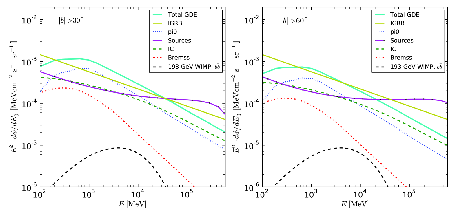
In Figure 1 we show the energy spectrum of the various Galactic and extra-galactic components for the model we employ. In particular, we show the average spectrum in the regions and , where the IGRB has the highest relative contribution. We show the power law fit to of the IGRB from [Abdo et al. 2009b]. Also shown is an example of extragalactic WIMP emission normalized to the model of Ullio et al. (2002) (with NFW halo profile and no halo substructures). The contribution from resolved point sources detected by Fermi [Abdo et al. 2009a],[Ballet 2009] is also present. It can be seen that, combined, these sources constitute a significant fraction of the diffuse background. For simplicity, the spectrum of each single source is modeled as a simple power law and thus the behavior at high energies ( GeV) may have some biases with respect to the real spectrum.
 |
 |
 |
3 Anisotropies: General Considerations
We will follow two approaches to quantify the anisotropies of all the gamma-ray sky components. For the components for which maps as a function of energy are available (i.e. for the Galactic foregrounds and for the resolved point sources) we calculate the angular power spectra directly from the maps using HEALpix [Gorski et al. 2005](see appendix A for more details on HEALpix and the definition of power spectra). For the remaining components (DM and astrophysical EGB) we model the power spectra from theory. From the theoretical power spectra we then also produce simulated sky-maps (under the assumption that the fluctuations are gaussian). In this way we have effective sky maps for all the components and we can combine them, convolve them with the Fermi IRFs, simulate finite statistics of events, apply masks, etc. The final maps will thus represent a simulated gamma-ray sky as seen through the Fermi detector and where all the components are entangled. Power spectra are then recovered at the end from the final maps using HEALpix. In this way the sensitivity to DM can be studied as described in section 7 by comparing the power spectra of the maps with and without the DM component.
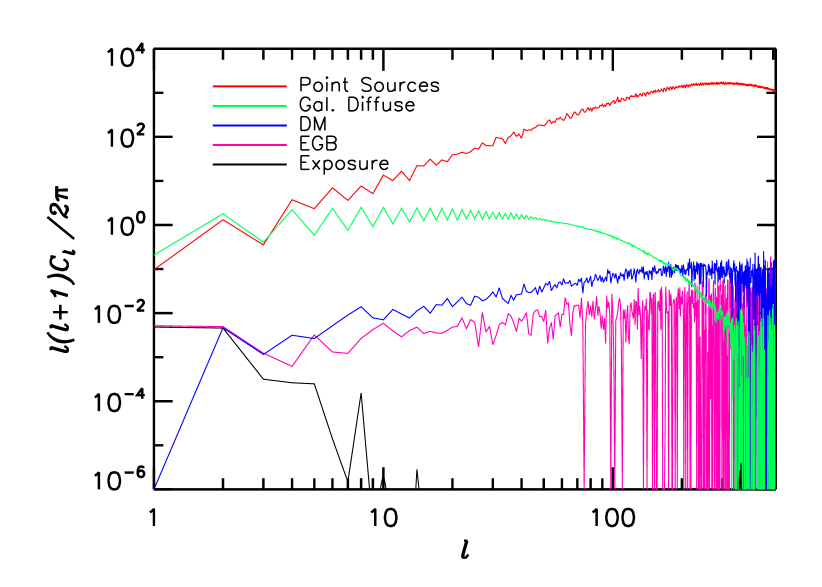
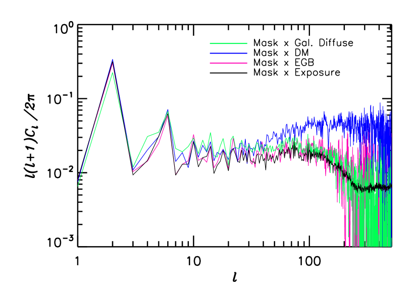
Fig.2 shows separately the all-sky angular spectra of the various components: Galactic foregrounds, astrophysical EGB, WIMPs EGB and point sources. The spectra are calculated from simulated maps at GeV after convolving with the Fermi IRFs (see the next sections). For illustrative purposes, the flux of the DM component is arbitrarily normalized to the level of the IGRB detected by Fermi and an observation time of 5 years is assumed. It can be seen that the Galactic foreground anisotropies have a decreasing spectrum in and dominate over the extragalactic anisotropies (either astrophysical or WIMP) up to . Luckily, however, this can be remedied using an appropriate mask excluding the Galactic plane region where most of the foregrounds are concentrated. In this way the foregrounds can be reduced such as to become subdominant at a multipole of as shown in the lowest panel of fig.2. The spectrum of point sources highly dominates both the foregrounds and the extragalactic signals. This indicates that an efficient point source masking is crucial to extract the interesting extragalactic signal. These steps will be explored in the next sections. The figure also illustrates the effect of the Poisson noise (first panel) coming from finite statistics present in the calculated raw power spectra. Customary power spectra are plotted with the noise removed (second panel).
The following section describes in detail how the power spectra of DM and astrophysical EGB are modeled and how the related maps are simulated. The section can be skipped by the reader not interested in these details.
4 Dark Matter and Astrophysical Anisotropies
4.1 Modeling the EGB
Apart the Poisson term coming from the unresolved point sources, the remaining source of anisotropies of the IGRB is given by the anisotropic spatial distribution of the sources themselves. To derive the anisotropy we will assume, as a reasonable first approximation, that the gamma ray sources are distributed as the matter density of the universe , i.e. following the cosmological Large Scale Structures (LSS). In principle , the density distribution of astrophysical sources, should be used instead of : in general exhibits a scale and time dependent bias with respect to the matter density. However, specific classes of astrophysical gamma-ray sources have different biases. For example, blazars are well known to concentrate at the center of clusters of galaxies, thus presenting an over-bias with respect to galaxies at high densities. On the other hand, galaxies and clusters of galaxies reasonably trace the matter density, at least in the recent cosmic epoch. The assumption is thus general enough to approximately describe emission from astrophysical sources.
Given these assumptions the extragalactic cosmic gamma-ray signal can be written as [Ullio et al. 2002, Bergstrom et al. 2001, Cuoco et al. 2006]
| (1) |
where is the photon spectrum of the sources, is the energy we observe today, is the matter density in the direction at a comoving distance , and the redshift is used as time variable. The Hubble expansion rate is related to its present value through the matter and cosmological constant energy densities as , and the reduced Hubble expansion rate is given by km/s/Mpc. We will in the following use , and km/s/Mpc. The quantity is the optical depth of photons to absorptions via pair production (PP) on the Extra-galactic Background Light (EBL). We use the parametrization of from [Stecker et al. 2006] for , where the evolution of the EBL is included in the calculation. The EBL is expected to be negligible at redshifts larger than corresponding to the peak of star formation. Thus, gamma photons produced at earlier times experience an undisturbed propagation until , while only in the recent epoch they start to lose energy due to scattering on the EBL. Correspondingly, we assume for (see also formula (A.6) in [Cuoco et al. 2006]).
In the case of cosmological DM annihilation, the resulting spatial distribution of the gamma signal follows the square of the matter distribution through
| (2) |
which, taking the spatial average, reduces to the expression
| (3) |
where is the clumpiness enhancement factor and is the average DM density at .
We can write the astrophysical EGB and DM in a compact form:
| (4) | |||||
| (5) |
where and are the astrophysical and DM window functions, which contain the information about gamma-ray propagation, injection spectra and cosmological effects
| (6) |
where applies in the astrophysical and DM cases, respectively and and are the boundaries of the energy bands considered. We are using the notation to underline that the window function is only dependent on the two variables, direction and redshift, and to make the behavior of the matter density explicit. In particular, choosing and , when properly normalized represents the probability of receiving a photon of emitted at a redshift . This can be used to define an effective horizon, , beyond which the probability of receiving a photon is negligible. In practice, above about 10 GeV, pair production attenuation sets the scale of the horizon which is about and for the cases respectively. In this case, DM annihilation produces a much larger anisotropy than the astrophysical sources. In contrast, below 10 GeV the horizon is set by cosmological effects and and for the two cases. In the low energy regime we thus see that the DM anisotropies are averaged over a much larger horizon and the final signal can be smoother than the astrophysical case. Further details are discussed in [Cuoco et al. 2007].
The injection energy spectrum for DM annihilation , given the annihilation channel and the WIMP mass , is calculated with DarkSUSY [Gondolo et al. 2004], which, in turn, uses a tabulation derived from simulation of the particle processes performed with Pythia [Sjostrand et al. 2007]. We will consider in the following the , and annihilation channels.
4.2 Angular Power Spectra
Given the above expressions we can write the angular power spectra of the various dimensionless fluctuation fields
| (7) | |||||
| (8) |
where we have used the Limber approximation [Limber 1953], which is accurate for all but the very lowest multipoles, while and are 3D power spectra of the matter field and of its square. We are also interested in the spectra of cross correlation among two different energy bands, which can be written as
| (9) |
where for the astrophysical and DM case.
We take the 3D power spectra and from an N-body simulation of Large Scale Structures formation [Cuoco et al. 2007]. We note that has a dependence on the clustering properties of DM below galactic scales (see [Ando & Komatsu 2006] for an analytical derivation of ) which are not resolved in the N-body simulation. The anisotropy properties in the case of cosmological DM annihilation with substructures are therefore not fully consistent with its energy spectrum normalization, which does take into account the effects of substructures. This has to be taken into account when interpreting the sensitivities in the cosmological substructures model shown in the following.
As described in the previous section we will consider in the following two different anisotropy models for the astrophysical EGB in order to bracket our uncertainties and estimate the effect on the DM sensitivity. The first one is a model dominated by the correlation term of the power spectrum (Eq.7), while the second one is a model dominated by the Poisson term from unresolved point sources. In this case the angular power spectrum is simply:
| (10) |
with .
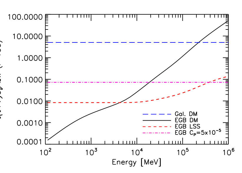
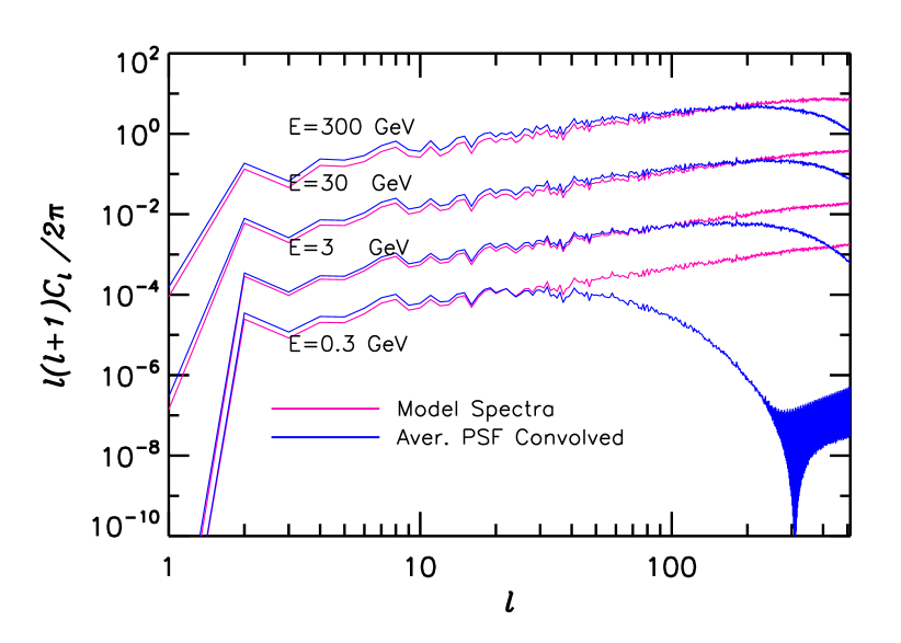
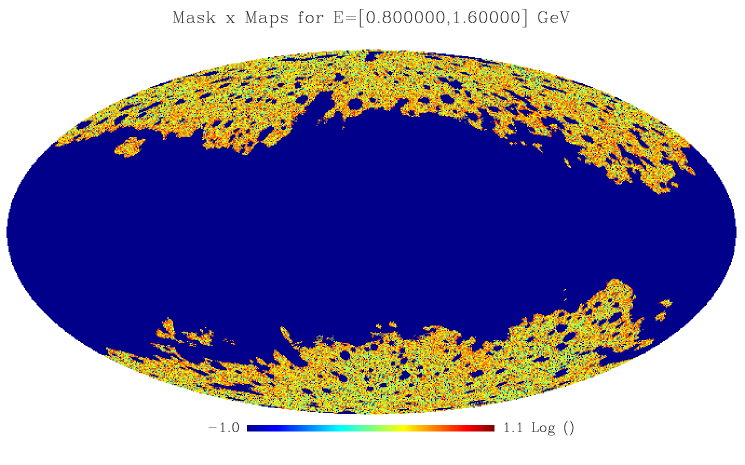
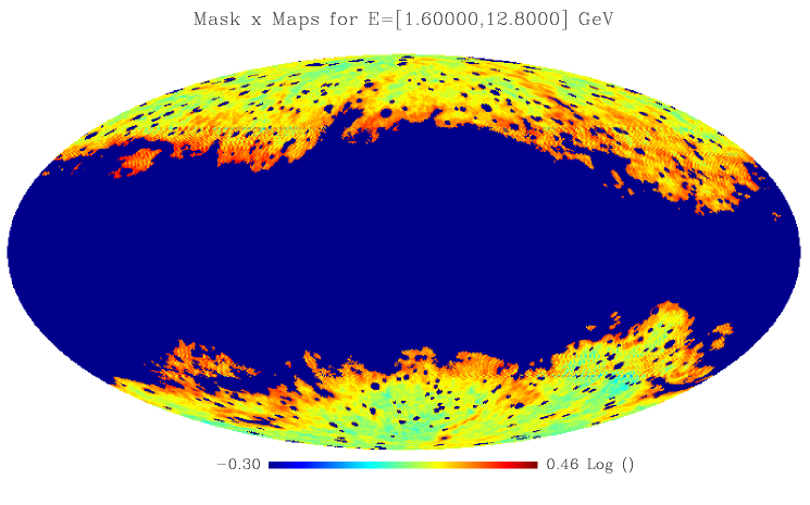
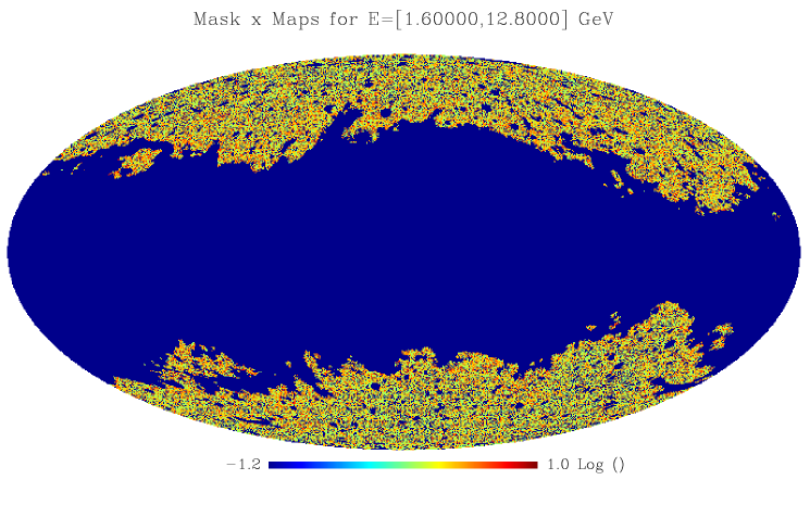
Finally we will also consider the possibility that part of the IGRB is produced by DM annihilation in the sub-structures of our galaxy as found by recent N-body simulations [Diemand et al. 2007, Springel et al. 2008a, Springel et al. 2008b]. In this case, compared to the cosmological annihilation scenario, the situation is simpler since, in the absence of redshift effects, the pattern of anisotropies is independent of energy (and thus of the particle physics model). This can be seen more clearly in Eq.6 where becomes a constant independent of energy and redshift. The anisotropies thus only depend on the clustering properties of DM in the Milky Way (MW). We will take as a reference model the from [Siegal-Gaskins 2008] where the anisotropies have been calculated from a simulated MW substructure map. In particular, we will use the spectrum shown in their Fig.5 for a minimum clump mass of . Compared with the cosmological DM anisotropies this model gives a normalization of the angular power spectrum a factor larger (or more) depending on the energy. More precisely, the shapes of the power spectra are similar for the two cases, while the absolute normalization for the Galactic case is at independent of energy, whereas for the extragalactic case at 10 GeV. Fig.3 shows the energy dependence of at for the various cases while Fig.4 shows for the DM EGB case for 4 different energies.
4.3 Model Sky Maps
To produce a realistic simulation of data from Fermi we have to simulate the expected sky pattern of every component. In the case of Galactic foregrounds we employ the GALPROP package [Strong and Moskalenko 1998, Moskalenko and Strong 1997] which produces as output the sky maps of the foregrounds as a function of energy. As already described above the conventional diffuse model is used. It is worth noticing that energy dependent CR diffusion effects imply an energy dependent sky pattern as well. In general, at low energies the diffusion length of CRs is large and the resulting maps are thus smoother than the higher energy counterparts where the diffusion length decreases. Thus the relative importance of the Galactic foregrounds anisotropies at small scales () increases with energy. Of course, projection effects along the line of sight can sometimes complicate the picture and give small scale anisotropies also at low energies although this in practice happens only along the Galactic plane where there is a contribution from structures many kpc away from the solar position.
For the remaining components, i.e. the astrophysical EGB and the DM
EGB, we create template maps as gaussian realizations of the
theoretical angular power spectra derived above. The situation
is however complicated by the fact that the angular spectra are
energy dependent and, further, that there are non-zero
cross-correlation power spectra between different energy bands.
Energy dependent maps with the correct cross-correlation properties
among different energies need thus to be realized. In practice, we
choose logarithmically spaced
energy bands between 10 MeV and 10 TeV (i.e 10 bands per energy
decade). We then calculate the angular auto-correlation power
spectra for each band and the cross-correlation power spectra
among all the possible pairs of energy bands according to equations
7-10. The result is the model
power spectrum matrix for the DM or
astrophysical EGB. We then generate the maps in harmonic space
(, (see definitions in the appendix)) up to
sampling from the 60x60 matrix of the multi-gaussian distribution given
by the for each . In practice the energy behavior is
generally highly correlated so that only the first 4-5
principal components are required for the simulation of the 60 maps.
The synfast tool from HEALpix is then employed to combine the harmonic components
into the real space maps . These energy
dependent anisotropy maps are then weighted and normalized at each
energy according to the energy spectrum of the component itself
(astrophysical or DM EGB), giving the final template maps. These can
now be added to the model of Galactic foregrounds and to the model of
point sources to give a simulation of the gamma-ray sky where all
the components are entangled.
For the case of Galactic DM the procedure is simpler given that the anisotropy pattern is independent of the energy and only one map needs to be simulated. The same holds for the astrophysical EGB model with pure Poisson noise.
Convolution with the instrumental effects is described in the next section.
5 The Fermi-LAT and simulated datasets
In the following we describe the various instrumental effects introduced in the Gamma-ray sky when observed through the eyes of the Fermi-LAT telescope.
5.1 Charged particles contamination
Charged particles, mainly protons, electrons and positrons, as well as a smaller number of neutrons and Earth albedo photons, present a major instrumental background to potential DM signals, in particular when considering the isotropic gamma-ray signal. These background particles greatly dominate the flux of cosmic photons incident on the LAT, and a multivariate technique, employing information from all LAT detector systems, is used to reduce the remaining charged particle background to only a fraction of the expected flux of extragalactic diffuse emission [Atwood et al. 2009]. The analysis of the extragalactic background from Fermi [Abdo et al. 2009b] however indicates that, with the standard data selection cuts, the residual contamination is comparable to the photon background itself above a few GeV and dominates at higher energies. Generally, this background is expected to be basically isotropic so it can be easily taken into account in the anisotropy analysis. Alternatively, stringent cuts can be applied on the photon events decreasing the contamination but also somewhat the exposure and thus the signal [Abdo et al. 2009b]. For our simulation we will use the effective area for the “diffuse” event class as defined in [Atwood et al. 2009]. Using more stringent selection cuts to reduce the effects of CR contamination reduces the effective area by a factor of 25% [Abdo et al. 2009b]. The sensitivity curves should change accordingly, approximately by the small factor . This estimate is reasonably accurate for a sensitivity study as the present one. We do not attempt a detailed simulation of the CR background itself, postponing a more careful investigation of the issue to the data analysis work.
5.2 Point Spread Function and Exposure
The effects of the Fermi-LAT detector can be summarized in terms of
the IRFs which include the point
spread function (PSF) and the energy dependent exposure maps. For
this analysis we use the PSF and exposure as available from the
Fermi Science tools p6v3 111See
http://fermi.gsfc.nasa.gov/ssc/ . We neglect the effect of energy
dispersion (which is about 10 %) and assume that the photon energy
is perfectly reconstructed. In this respect, for this analysis we
will divide the simulated datasets in wide energy bands so that this
instrumental effect is negligible for our purposes. To obtain
simulated maps we use the energy dependent model input maps and then
convolve them with the Fermi PSF and simulated exposure of 5 years.
More specifically, the exposure was generated from 1 yr of pointing history
simulated with gtobssim and then rescaled to 5 yrs. The convolution with the PSF and the exposure
was then performed using the GaDGET [Ackermann et al. 2009] tool (see also Abdo et al. (2009b)).
The resulting maps have a normalization in units of counts per
steradian which is further re-normalized to counts per pixel (sr for a Nside=256 HEALpix pixelization). Finally Poisson
random noise is added to simulate the effect of finite statistics.
The Fermi PSF is energy dependent and improves at high energies. It corresponds to an angular resolution of about at 100 MeV, at 1 GeV and above 10 GeV (see [Atwood et al. 2009] for more details). The PSF thus heavily affects the anisotropies especially below 1 GeV, suppressing the medium-high multipoles in the angular power spectrum. The sensitivity to these multipoles is not completely lost however. In principle, from the knowledge of the PSF it is possible to recover the true power spectrum even at higher multipoles although the error grows with larger attenuation (it grows exponentially with multipole : the suppression factor is given by , for a gaussian PSF with variance ).
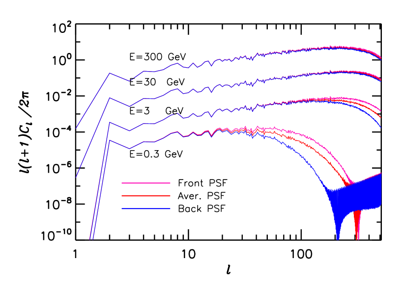
The effect of the PSF can be seen in Fig.4 where our model power spectra for the DM EGB component at various energies are compared with the corresponding PSF convolved spectra. The latter are obtained by convolving the model DM EGB sky maps (simulated from the angular spectra with the procedure described in the previous section) with the PSF and extracting the power spectra from the resulting maps. As expected, the PSF heavily suppresses anisotropies at for E1GeV. Notice also that there is a certain suppression at even for GeV, which is slightly more than the factor expected at this energy for a gaussian PSF with width . This extra effect is likely related to the non-gaussian form of the PSF which even at very high energies ( GeV) exhibits a tail towards large angular spreads. The figure also shows the difference in PSF for events converting in the front or the back of the detector where the reconstruction performances are different. It can be seen that the PSF is better for events converting in the front, giving a sensitivity to slightly higher multipoles especially at low energies. Above a few GeV, instead, the difference is less important. We will use the average PSF for our analysis.
The exposure maps are very uniform over an averaging period of 1 year (see again [Atwood et al. 2009]) so that the convolution with the exposure only adds power to the very lowest multipoles . This can seen in fig.2 where we plot the angular power spectrum of the exposure which, indeed, falls rapidly at . The exposure pattern is also energy dependent, although only weakly. The integrated exposure, however, rises steeply starting from about 100 MeV and then flattens above about 1 GeV.
 |
 |
 |
 |
 |
 |
 |
 |
 |
 |
 |
 |
6 Results of the Simulation
6.1 Simulated Sky-Maps
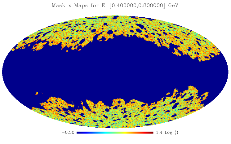
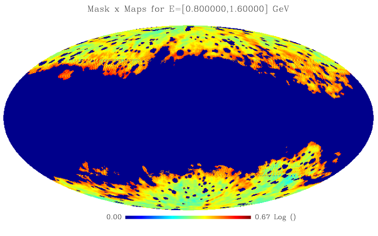
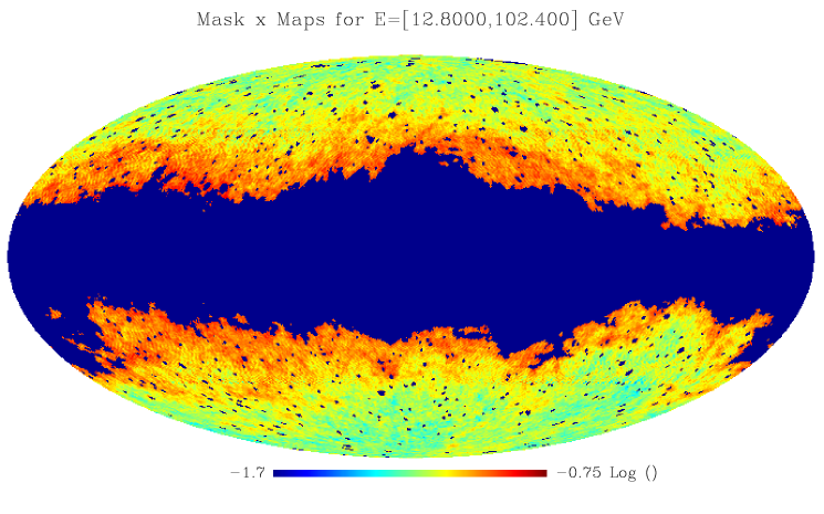
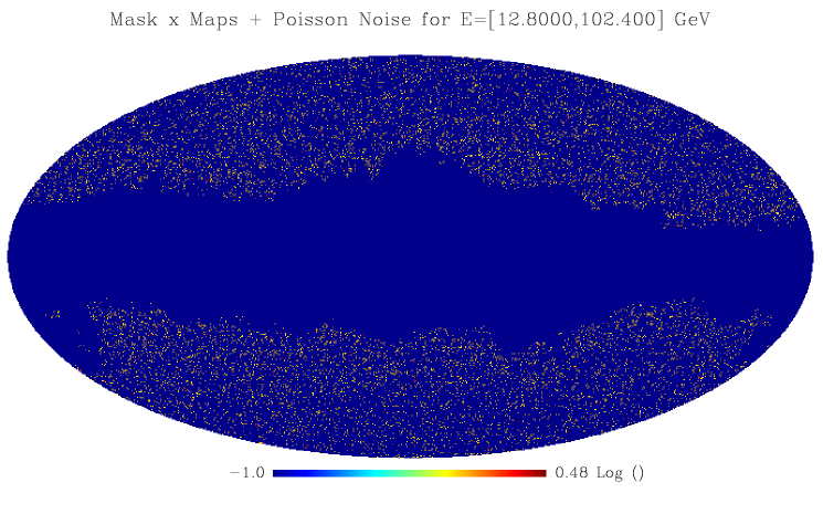
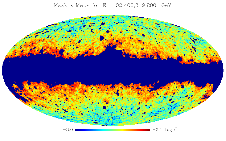
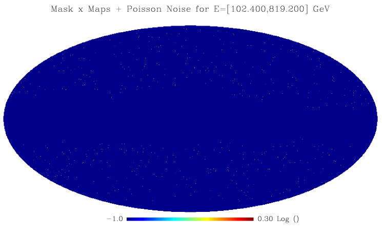
The maps produced as described in the previous sections are summed up to build a simulation of the observed gamma-ray sky. A reference no-DM model is derived adding Galactic foregrounds, astrophysical EGB and point sources. The astrophysical EGB is normalized to the level of the observed IGRB. The normalization of the Galactic foregrounds is the one given as output by GALPROP. Point sources are normalized to their observed flux. The overall statistics is normalized to 5 years of data taking by Fermi. The maps we obtain are average counts maps, but a realization of effective counts maps can be easily obtained drawing poisson counts in each pixel from the average counts maps. Although we use 60 energy bands to produce the simulated maps, it is convenient to rebin them into fewer maps, in order to have a reasonable amount of statistics in each band. We thus divide the dataset in 5 energy bands from 400 MeV to 800 GeV. Finally, a crucial step is the construction of the masks which will suppress the Galactic foregrounds and the resolved point sources. For each energy band the mask are defined as the region where the foregrounds do not exceed twice the EGB (200%), and the point sources emission does not exceed more than 20% of the EGB itself. Simulated sky maps (outside the masked regions) for both the average counts and one particular realization of the counts are shown in Fig.5. Indeed, outside the masks the remaining signal is quite isotropic, indicating that the IGRB makes most of the signal, but still a certain residual foreground contamination is apparent, especially near the edges of the mask. Clearly this is expected given the loose cut employed to build the masks (only 200% of the EGB). A tighter cut on the foregrounds can be applied but then the available area for the analysis would shrink to close to zero since the Galactic foregrounds never go below 20-30% of the EGB even at the Galactic poles. For the present forecast analysis a substantial foreground contamination is still acceptable since the foreground model is known in advance and what is required for a significant detection is that the EGB anisotropy exceeds the anisotropy of the residual Galactic foregrounds. In general, for a real data analysis some kind of foreground cleaning must be performed to obtain useful results. We postpone a detailed treatment of this issue to the analysis of the real data.
On the other hand, the cut of 20% of the EGB for point sources is rather effective and removes most of the gamma-ray events from resolved point sources, except perhaps few events around the most powerful sources where, statistically, some events very far from the source position are expected due to the tails of the PSF. From Fig.5 it can also be seen that the fraction of sky where the isotropic component dominates increases with energy. This is expected considering the fact that the IGRB has a spectrum harder than the Galactic emission (see also Fig.1). Also it is clear that the area masked for the point sources substantially decreases at high energy due to the improvement of the PSF. This is true for all but the highest energy band, where the fraction of sky covered by the point sources increases again. This can be understood looking at the energy spectrum of the resolved sources in Fig.1. This becomes very hard for GeV so that, even if the PSF at this energies is very narrow, its tail still contains a flux which is a significant fraction of the IGRB.
6.2 Angular Power Spectra
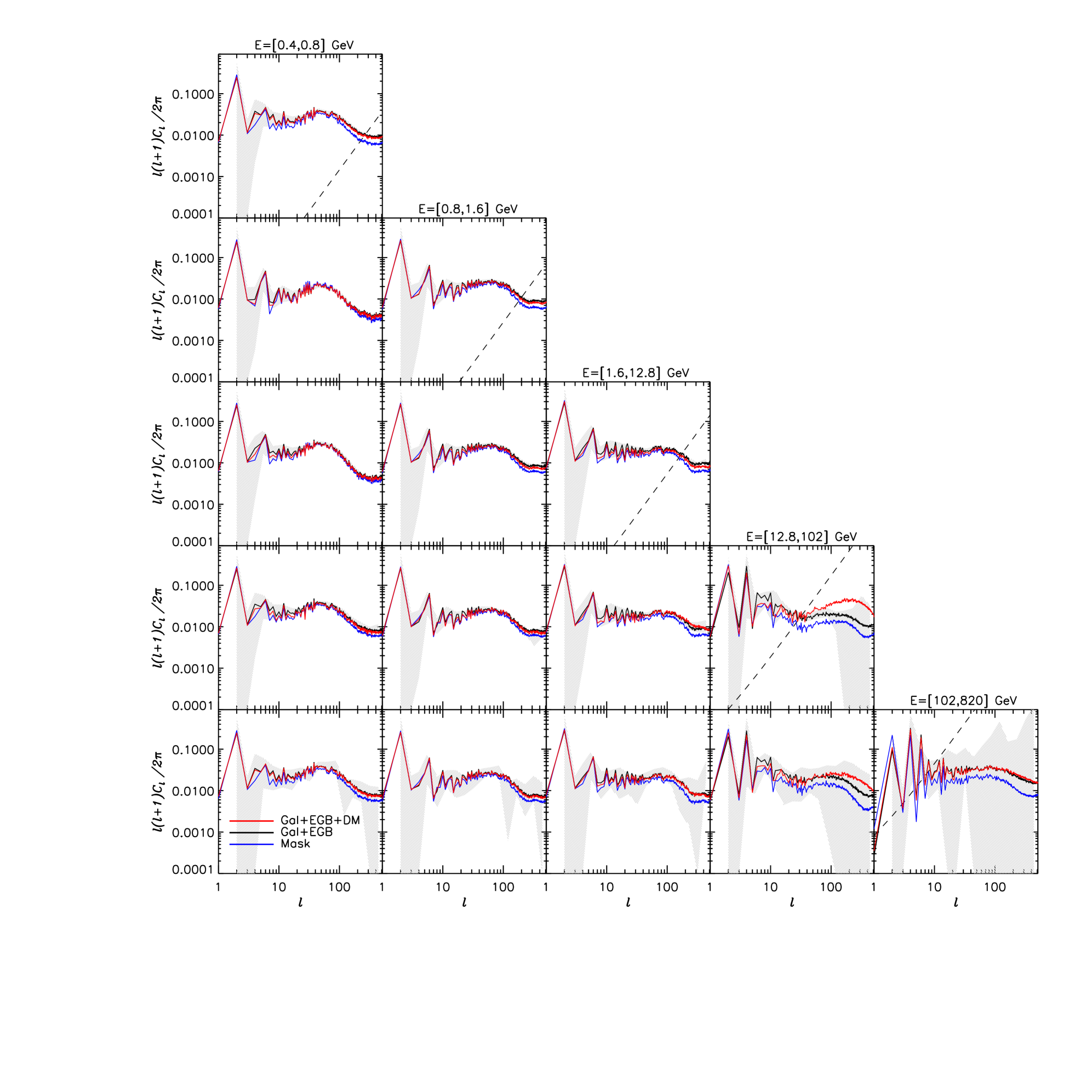
In Fig.6 we plot the various auto-correlation and cross-correlation spectra in a “triangle plot”, where the diagonal represents the auto-correlations and the the off-diagonals the cross-correlations. The blue lines represent the spectra of the masks only, which thus provide the zero-level anisotropy. The black line represents the average spectrum of the reference no-DM model convolved with masks, i.e. the maps in the left column in Fig.5. As explained above, outside the mask the reference model is to a large extent given by the astrophysical EGB, although a substantial residual contamination from the Galactic foregrounds is still present. The residual point source contamination, on the other hand, is negligible. The grey shaded area is the two sigma error region in the power spectrum accounting for the effect of the finite number of events. A logarithmic binning of the multipoles in 18 bands is used. The level of shot noise is shown with a dashed line. It can be seen that the shot noise increases in the high energy bands where the statistics decrease, as expected. Finally, the red curves represent the angular power spectra if a EGB DM component is added on top of the previous contributions. For illustration a WIMP with GeV is chosen and the DM flux is normalized to the same level of the EGB at 10 GeV. It can be seen, indeed, that in the 4th energy band (approximately 10-100 GeV), where the DM emission peaks, the anisotropy has a noticeable bump compared to the EGB anisotropy and provides a clear signature for this model. The DM anisotropy signal disappears in the 5th band (100-800 GeV) where the DM contribution drops. This “energy modulation in the anisotropy spectrum” is also discussed in [Hensley et al. 2009]).
It has to be noted that the spectra look quite different from the all-sky spectra of the astrophysical and DM EGB shown in Fig.2, both in the shape and normalization. This is of course due to the effects of the residual foregrounds and especially of the mask which distorts the original spectrum. The mask effects can in principle be removed with specifically designed algorithms like the MASTER algorithm [Hivon et al. 2002]. This comes, however, at the price of further errors in the final spectrum which need to be addressed with Montecarlo simulations (a package implementing the full procedure is described for example in [Lewis 2008] ). For the present purpose, it suffices to use the masked sky power spectrum without attempting to deconvolve it from the mask itself. This is fine as long as all the power spectra are calculated on the same sky region in order to allow a consistent treatment.
 |
 |
 |
7 DM sensitivity
It is in principle straightforward to calculate the sensitivity to DM requiring that the DM anisotropy does not exceed the anisotropies of the reference no-DM model. Let us define as the binned multipoles power auto- and cross-correlation spectra of the reference model 222We label it for simplicity EGB although, besides the true astrophysical EGB, there are some residual contaminations from Galactic foregrounds and point sources (see previous section).. The indices run from 1 to 5 and indicate the energy bands and the index indicates the multipoles bins. Let us also define as the covariance matrix of the , i.e. is the covariance between and . We divide the multipole range into 18 logarithmically spaced multipole bands. Adding to the previous signal, the contribution for a given DM model, specified through the annihilation channel, the velocity averaged annihilation cross section and the DM mass, we further obtain which can be compared with the no-DM hypothesis as:
| (11) |
where is the inverse of the covariance matrix. As a first step, however, we might want to consider a simple expression, for example considering as observables only the auto-correlation spectra . Unfortunately, the naive expression
| (12) |
turns out to be incorrect because the two spectra and are correlated, i.e. . The correlation, indeed, is given by , i.e. by the cross correlation between the bands and , as intuitively expected. The variance of can be also easily calculated and gives , where is the poisson shot noise. The correct expression is then
| (13) |
where is the inverse of and
| (14) | |||||
| (15) |
To take into account multipole binning and partial sky coverage, in the above expressions we have to substitute
| (16) |
where is the number of binned multipole in the band l’, and is the density of the counts per steradian. Notice that in the above formulae no corrections for the angular resolution (the term) are required since we are referring to raw, PSF uncorrected spectra. Finally, we disregard the information at to minimize the effects of the exposure. Let us also notice that, after all, the value of calculated with Eq.12 turns out to be generally similar to the one of Eq.13. This behavior may be due to the different levels of noise in the various energy bands and in the autocorrelation spectra which makes the off-diagonal components in the covariance matrix (which do not have shot noise) generally subdominant.
In case we want to exploit all the available information, i.e. including both the auto-correlations and the cross-correlations as observables, the full expression Eq.11 for the has to be employed. In this case the full covariance matrix becomes more complicated and we give the corresponding expressions in appendix B.
Some further comments are in order regarding the calculation of . We use always the same set of DM anisotropy maps to calculate the s for the cosmological DM case, despite the fact that they in principle depend on (and the annihilation mode) through Eqs.6 and 7. Consequently, a different set of maps should be generated for each value of and for each channel. Fortunately, this dependence is weak above about 10 GeV where the DM horizon does not depend much on the DM annihilation energy spectrum so the effects on the sensitivity plots above 10 GeV are small, accordingly. To better justify this approximation we can also make a comparison with the case of DM annihilation from substructures in the Galactic halo where we use a very different set of maps. The sensitivities generally change by a factor of a few in this case (see below). The slight dependence of the maps on DM model for the cosmological case is thus likely to be smaller than that.
 |
 |
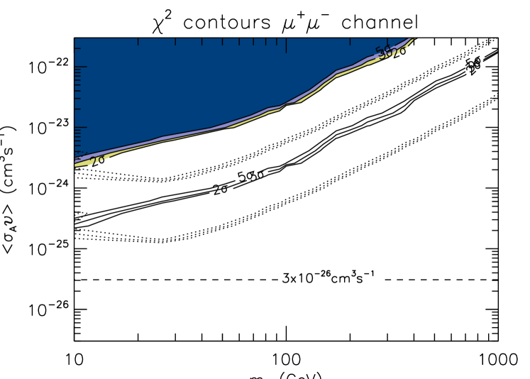 |
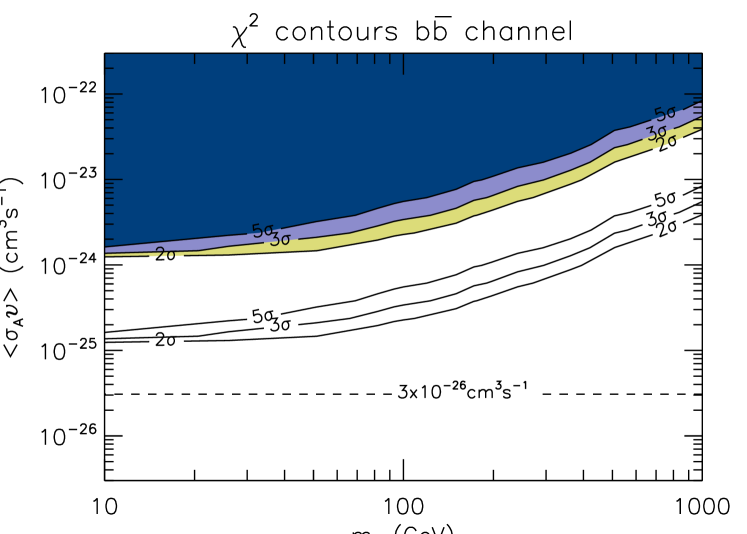
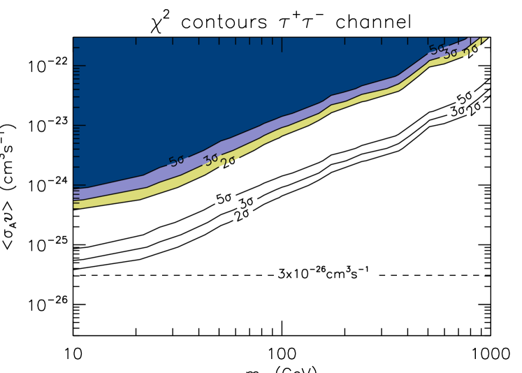
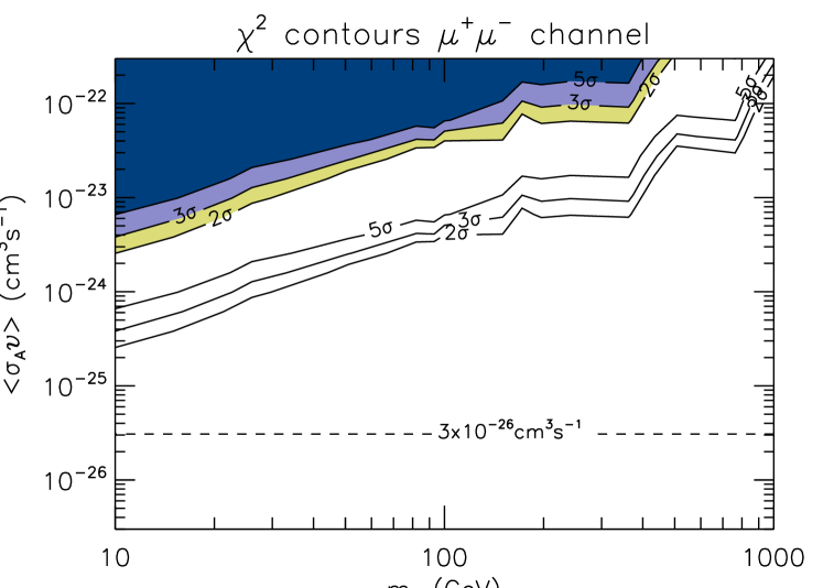
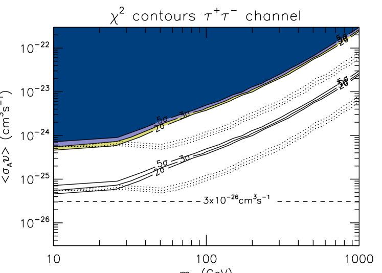
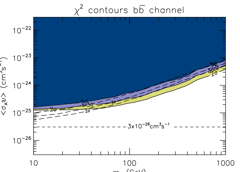
We can see the results in Fig. 7, where the sensitivities are reported for various annihilation channels. The absolute normalization of the DM spectra are obtained following the DM haloes clustering model of [Ullio et al. 2002] as described in the introduction. Two versions of the model are shown: a conservative version with a NFW profile for the haloes and no substructures which gives a low DM normalization, and thus weaker constraints, and a more optimistic version where the DM signal is enhanced by the presence of substructures in the DM haloes. In principle, using the recent results of[Zavala et al. 2009] from the Millenium-II simulation, an order of magnitude enhancement with respect to the above “optimistic” case can be achieved with a correspondingly better sensitivity (see also [Abdo et al. 2010a], in particular Fig.1).
The various channels have generally similar behavior. The channel produces quite smooth limits. The and sensitivity curves in contrast have a steeper slope and exhibit more structure. This is due to the fact that for these channels the gamma emission is concentrated at higher energies in a narrow peak near the energy corresponding to the DM mass. The sensitivity is thus more sensitive to the coarse binning in energy chosen for this analysis. The sensitivity in the channel and especially the channel at higher DM masses somewhat decreases due to the lower number of photons per annihilation (and thus lower statistics) available.
Including the cross-correlation spectra information does not seem to improve the sensitivity. This probably has to be ascribed to the fact that the for the auto-correlation case already includes some cross-correlation information in the off-diagonal terms of the covariance matrix. The level of anisotropies is also very low at low energy for this case (see Fig.3) and this somewhat reduces the importance of the information contained in the cross-correlation. The situation is different for the Galactic DM scenario as discussed below.
We also checked the case in which only the highest energy bands are employed for the analysis. We would expect an improvement in sensitivity given that very little DM signal is expected in the 0.4-0.8 GeV band and thus scanning in this energy range introduces a statistical penalty factor. We find that the sensitivity indeed improves, but only marginally. On the other hand, the lowest energy band is useful because being mostly clean of DM it represents a good calibration for the background anisotropies.
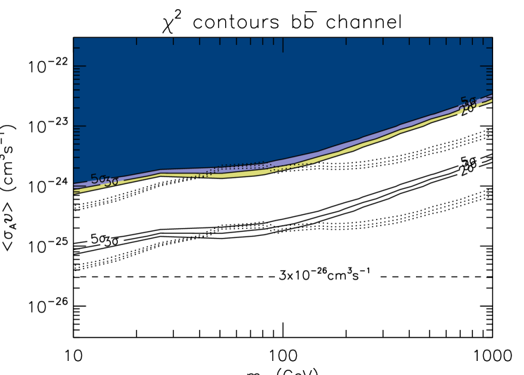
In Fig. 8 we show the case in which the DM anisotropy pattern does not vary with energy. This case is supposed to mimic the DM emission from unresolved substructures in the Milky Way. We thus simulate a single anisotropic map which we use for all energies. The angular spectrum for DM employed to simulate the map is normalized as in the case of substructures with a minimum mass of 10 as derived in [Siegal-Gaskins 2008] and it roughly corresponds to the extragalactic anisotropies for an energy of about 300 GeV (see section 2). For a direct comparison with the cosmological case we use for the Galactic signal the same normalization employed for the extragalactic case, which is justified by the fact that more physically motivated models for the DM emission in the MW have a large degree of freedom [Ando 2009] and can easily be tuned to match the extragalactic case.
The inclusion of the information from the cross-correlation spectra in this case, contrary to the cosmological one, gives a significant improvement, especially for higher DM masses. The reason for this difference is likely to be found in the very different set of anisotropy maps employed for the Galactic substructures case. In particular, the very high degree of anisotropy present also at low energy for this case enhances the importance of a direct measurement of the cross-correlation between low and high energy bands. In contrast, the very low DM anisotropy at low energy for the cosmological case (lower than the astrophysical EGB anisotropy) makes this information almost irrelevant. We also find in this case that excluding the lowest energy band does not improve the sensitivity significantly.
The sensitivity increases substantially with respect to the cosmological case, especially for high DM masses. The slope of the sensitivity curves is indeed slightly less steep. Assuming higher levels of anisotropy for the Galactic case, which are possible, [Ando 2009, Siegal-Gaskins 2008, Siegal-Gaskins and Pavlidou 2009] a correspondingly higher sensitivity could be achieved. However, the scaling is not linear. It is worth noting for example that although at about 10 GeV the Galactic anisotropies are about 2 orders of magnitudes larger than the extragalactic ones, the sensitivity is only a factor 2-3 better. The scaling however is better for GeV where the difference in sensitivity is roughly a factor of 10. This non linear scaling is due to the limited limited amount of detected photons (as it is the case at the edges of the sensitivity curve). Here, it is very difficult to distinguish between the two (galactic and extra-galactic) levels of anisotropies even if the latter is a factor 100 larger, since the statistical error bars are also very large. The much larger galactic anisotropy thus only modestly decrease the minimum amount of events required to detect the signal.
Finally in Fig. 9 we show the impact on the DM sensitivity of changing the underlying astrophysical EGB model to the Poisson dominated one. For illustration, only the extragalactic case with NFW profile and substructures is shown. The interesting results (perhaps somewhat counter intuitive) is that even with this increased level of background in the anisotropy spectrum, still the sensitivity to the DM component remains roughly unchanged. The reason is that a Poisson noise at the level of 5.0e-5 is anyway clearly detected with a statistics of 5 years, so the DM component can still be easily detected as a modulation (as usual, in multipole and in energy) of this dominant Poisson noise anisotropy spectrum. The underlying assumption here, however, is that this new background is fully under control and well characterized. The extent to which this will be true is however not clear and a better understanding may require dedicated simulations and analyses which are beyond the scope of this paper.
8 Summary and Conclusions
In the present analysis we have calculated the sensitivity to Dark Matter annihilation exploiting the characteristic anisotropy properties that DM would imprint in the Extra-Galactic Gamma Background. We performed a realistic simulation of the Fermi-LAT including the effect of the Point Spread Function, effective area and of the anisotropic sky exposure.
More importantly, we investigated the impact of Galactic foregrounds on the DM anisotropy sensitivity using a GALPROP model to produce the sky maps of the Galactic gamma emission. The contribution of Galactic foregrounds is generally non negligible even above Galactic latitudes of about . Foreground cleaning will thus be an important (and likely challenging) issue in the analysis of the real data. For the present work we do not attempt foreground cleaning (except for masking the Galactic plane and point sources) and we only require that the anisotropy from DM has to exceed the level of foregrounds anisotropy to be detectable. Further, we only analyze a high Galactic latitude region where the model dependence of the foreground is expected to be moderate. In this respect our analysis can be regarded as a conservative one: In reality, if foreground cleaning can be effectively implemented, a sensitivity to a lower level of anisotropy can be achievable. Also, a larger fraction of the sky can be employed than the small conservative one used in the present analysis. We leave a more careful investigation of the issue for future work.
Despite the difficulties involved in the foreground analysis, we find that the prospects for detecting DM anisotropy signatures are promising. For some WIMP masses, sensitivity to cm3s-1(i.e. the thermal relic value) can be achieved using the anisotropy information alone. Interestingly, these constraints are comparable to what is achievable using the energy spectrum alone [Abdo et al. 2010a] . The anisotropy information is thus complementary to the energy spectrum and provides a cross-check and an increase in the overall sensitivity to the DM signal.
We also investigated the recently proposed scenario of a population of DM substructures in the Milky Way halo as predicted by N-body simulations. These subhaloes give rise to an annihilation signal which is almost uniform in the sky and which can be comparable in intensity to the observed isotropic gamma background. For this case, the anisotropy signal is predicted to be even higher than for the extragalactic case due to the huge clumpiness of the DM distribution that correspondingly gives an enhanced sensitivity. We find, indeed, that when increasing the anisotropy the sensitivity to the DM signal increases as well with an improvement of a factor of 10 for GeV.
In summary, simulations indicate that ,with the sensitivity of the Fermi-LAT, detailed anisotropies studies of the gamma-ray sky can be performed. The next obvious step will be the analysis of the actual data. Anisotropy analyses will soon provide a complementary source of information which will give further insights into the DM problem and the properties of high-energy astrophysical sources.
Acknowledgments
The authors would like to thank Toby Burnett, Jennifer Siegal-Gaskins and Eiichiro Komatsu for their numerous comments and suggestions for improvement, and Chris Savage for a carefully reading of the manuscript. We also wish to thank Gianfranco Bertone for organizing the workshop “Gamma in Zurich” which stimulated many interesting discussions on gamma-ray anisotropies.
The Fermi LAT Collaboration acknowledges generous ongoing support from a number of agencies and institutes that have supported both the development and the operation of the LAT as well as scientific data analysis. These include the National Aeronautics and Space Administration and the Department of Energy in the United States, the Commissariat à l’Energie Atomique and the Centre National de la Recherche Scientifique / Institut National de Physique Nucléaire et de Physique des Particules in France, the Agenzia Spaziale Italiana and the Istituto Nazionale di Fisica Nucleare in Italy, the Ministry of Education, Culture, Sports, Science and Technology (MEXT), High Energy Accelerator Research Organization (KEK) and Japan Aerospace Exploration Agency (JAXA) in Japan, and the K. A. Wallenberg Foundation, the Swedish Research Council and the Swedish National Space Board in Sweden.
Additional support for science analysis during the operations phase is gratefully acknowledged from the Istituto Nazionale di Astrofisica in Italy and the Centre National d’Études Spatiales in France.
References
- [Abdo et al. 2009a] A. A. Abdo et al. [Fermi LAT Collaboration], Astrophys. J. Suppl. 183 (2009a) 46 [arXiv:0902.1340 [astro-ph.HE]].
- [Abdo et al. 2009b] A. A. Abdo et al. [Fermi LAT Collaboration], arXiv:1002.3603 (2009b).
- [Abdo et al. 2009c] A. A. Abdo et al. [Fermi LAT Collaboration], Phys. Rev. Lett. 103 (2009c) 251101 [arXiv:0912.0973 [astro-ph.HE]].
- [Abdo et al. 2009d] A. A. Abdo et al. [Fermi LAT Collaboration], arXiv:1002.2280 (2009d).
- [Abdo et al. 2010a] A. A. Abdo et al. [Fermi-LAT Collaboration], arXiv:1002.4415 (2010a).
- [Abdo et al. 2010b] A. A. Abdo et al. [Fermi-LAT Collaboration], arXiv:1003.0895 (2010b).
- [Ackermann et al. 2009] M. Ackermann, G. Johannesson, S. Digel, I. V. Moskalenko, T. Porter, O. Reimer and A. Strong [Fermi LAT Collaboration], AIP Conf. Proc. 1085 (2009) 763.
- [Ando 2009] S. Ando, arXiv:0903.4685 [astro-ph.CO].
- [Ando & Komatsu 2006] S. Ando and E. Komatsu, Phys. Rev. D 73 (2006) 023521 [arXiv:astro-ph/0512217].
- [Ando & Pavlidou 2009] S. Ando and V. Pavlidou, Mon. Not. Roy. Astron. Soc. 400 (2009) 2122 [arXiv:0908.3890 [astro-ph.HE]].
- [Ando et al. 2006] S. Ando, E. Komatsu, T. Narumoto and T. Totani, Mon. Not. Roy. Astron. Soc. 376 (2007) 1635 [arXiv:astro-ph/0610155].
- [Ando et al. 2007] S. Ando, E. Komatsu, T. Narumoto and T. Totani, Phys. Rev. D 75 (2007) 063519 [arXiv:astro-ph/0612467].
- [Atwood et al. 2009] W. B. Atwood et al. [LAT Collaboration], Astrophys. J. 697 (2009) 1071 [arXiv:0902.1089 [astro-ph.IM]].
- [Ballet 2009] J. Ballet [Fermi Collaboration], Talk Given at the Washington Fermi Symposium 2009
- [Baltz et al. 2008] E. A. Baltz et al., JCAP 0807 (2008) 013 [arXiv:0806.2911 [astro-ph]].
- [Bergstrom 2000] L. Bergstrom, Rept. Prog. Phys. 63 (2000) 793 [arXiv:hep-ph/0002126].
- [Bergstrom et al. 2001] L. Bergstrom, J. Edsjo and P. Ullio, Phys. Rev. Lett. 87, 251301 (2001) [astro-ph/0105048].
- [Bertone et al. 2004] G. Bertone, D. Hooper and J. Silk, Phys. Rept. 405 (2005) 279 [arXiv:hep-ph/0404175].
- [Cuoco 2008] A. Cuoco, PoS IDM2008 (2008) 114.
- [Cuoco et al. 2006] A. Cuoco, S. Hannestad, T. Haugbolle, G. Miele, P. D. Serpico and H. Tu, JCAP 0704 (2007) 013 [arXiv:astro-ph/0612559].
- [Cuoco et al. 2007] A. Cuoco, J. Brandbyge, S. Hannestad, T. Haugboelle and G. Miele, Phys. Rev. D 77 (2008) 123518 [arXiv:0710.4136 [astro-ph]].
- [Diemand et al. 2007] J. Diemand, M. Kuhlen and P. Madau, halo,” Astrophys. J. 657 (2007) 262 [arXiv:astro-ph/0611370].
- [Dodelson et al. 2009] S. Dodelson, A. V. Belikov, D. Hooper and P. Serpico, arXiv:0903.2829 [astro-ph.CO].
- [Faucher-Giguere & Loeb 2009] C. A. Faucher-Giguere and A. Loeb, arXiv:0904.3102 [astro-ph.HE].
- [Fornasa et al. 2009] M. Fornasa, L. Pieri, G. Bertone and E. Branchini, arXiv:0901.2921 [astro-ph].
- [Gabici and Blasi 2002] S. Gabici and P. Blasi, Astropart. Phys. 19, 679 (2003) [astro-ph/0211573].
- [Gondolo et al. 2004] Gondolo P., Edsjo J., Ullio P., Bergstrom L., Schelke M. and Baltz E.A., JCAP 0407 (2004) 008 [astro-ph/0406204].
- [Gorski et al. 2005] K. M. Gorski, E. Hivon, A. J. Banday, B. D. Wandelt, F. K. Hansen, M. Reinecke and M. Bartelman, Astrophys. J. 622 (2005) 759 [arXiv:astro-ph/0409513].
- [Hartman et al.(1999)] Hartman, R. C., et al. 1999, VizieR Online Data Catalog, 212, 30079
- [Hensley et al. 2009] B. S. Hensley, J. M. Siegal-Gaskins and V. Pavlidou, arXiv:0912.1854 [astro-ph.CO].
- [Hivon et al. 2002] E. Hivon, K. M. Gorski, C. B. Netterfield, B. P. Crill, S. Prunet and F. Hansen, Astrophys. J. 567 (2002) 2, arXiv:astro-ph/0105302.
- [Hooper & Serpico 2007] D. Hooper and P. D. Serpico, JCAP 0706 (2007) 013 [arXiv:astro-ph/0702328].
- [Hunter et al. 1997] Hunter S.D. et al., Astrophys. J. 481 (1997) 205.
- [Ibarra et al. 2010] A. Ibarra, D. Tran and C. Weniger, Phys. Rev. D 81 (2010) 023529 [arXiv:0909.3514 [hep-ph]].
- [Jungman et al. 1995] G. Jungman, M. Kamionkowski and K. Griest, Phys. Rept. 267 (1996) 195 [arXiv:hep-ph/9506380].
- [Kalashev et al. 2007] O. E. Kalashev, D. V. Semikoz and G. Sigl, Phys. Rev. D 79 (2009) 063005 [arXiv:0704.2463 [astro-ph]].
- [Keshet et al. 2003] U. Keshet, E. Waxman, A. Loeb, V. Springel and L. Hernquist, Astrophys. J. 585 (2003) 128 [arXiv:astro-ph/0202318].
- [Komatsu at al. 2008] E. Komatsu et al. [WMAP Collaboration], arXiv:0803.0547 [astro-ph].
- [Lee et al. 2008] S. K. Lee, S. Ando and M. Kamionkowski, arXiv:0810.1284 [astro-ph].
- [Lewis 2008] A. Lewis, Phys. Rev. D 78 (2008) 023002 [arXiv:0804.3865 [astro-ph]].
- [Limber 1953] D. N. Limber, Astrophys. J. 117 (1953)
- [Navarro et al. 1995] J. F. Navarro, C. S. Frenk and S. D. White, Astrophys. J. 462 (1996) 563
- [Miniati et al. 2007] F. Miniati, S. M. Koushiappas and T. Di Matteo, Astrophys. J. 667 (2007) L1 [arXiv:astro-ph/0702083].
- [Moskalenko and Strong 1997] Moskalenko I.W. and Strong A.W., Astrophys. J. 493 (1998) 694
- [Pavlidou and Fields 2002] V. Pavlidou and B. D. Fields, Astrophys. J. 575, L5 (2002) [astro-ph/0207253].
- [Pieri et al. 2007] L. Pieri, G. Bertone and E. Branchini, Mon. Not. Roy. Astron. Soc. 384 (2008) 1627 [arXiv:0706.2101 [astro-ph]].
- [Pieri et al. 2009] L. Pieri, J. Lavalle, G. Bertone and E. Branchini, arXiv:0908.0195 [astro-ph.HE].
- [Porter 2009a] T. A. Porter [Fermi Collaboration], arXiv:0907.0294 [astro-ph.HE].
- [Porter 2009b] T. A. Porter [Fermi Collaboration], Talk Given at TeV Particle Astrophysics 2009
- [Siegal-Gaskins 2008] J. M. Siegal-Gaskins, JCAP 0810 (2008) 040 [arXiv:0807.1328 [astro-ph]].
- [Siegal-Gaskins and Pavlidou 2009] J. M. Siegal-Gaskins and V. Pavlidou, arXiv:0901.3776 [astro-ph.HE].
- [Siegal-Gaskins 2010] J. M. Siegal-Gaskins, for the Fermi-LAT Collaboration and E. Komatsu, [arXiv:1012.1206 [astro-ph.HE]].
- [Sjostrand et al. 2007] Sjostrand T., Mrenna S. and Skands P., Comput. Phys. Commun. 178 (2008) 852 [arXiv:0710.3820].
- [Springel et al. 2008a] V. Springel et al., arXiv:0809.0894 [astro-ph].
- [Springel et al. 2008b] V. Springel et al., arXiv:0809.0898 [astro-ph].
- [Sreekumar et al. 1998] Sreekumar P. et al. [EGRET Collaboration], Astrophys. J. 494 (1998) 523 [astro-ph/9709257].
- [Stecker and Salamon 1996] F. W. Stecker and M. H. Salamon, Astrophys. J. 464, 600 (1996) [astro-ph/9601120].
- [Stecker et al. 2006] F. W. Stecker, M. A. Malkan and S. T. Scully, Astrophys. J. 648, 774 (2006) [astro-ph/0510449]. See also F. W. Stecker, M. A. Malkan and S. T. Scully, Astrophys. J. 658 (2007) 1392 [arXiv:astro-ph/0612048].
- [Stecker et al. 2008] F. W. Stecker, S. D. Hunter and D. A. Kniffen, Astropart. Phys. 29 (2008) 25 [arXiv:0705.4311 [astro-ph]].
- [Strong and Moskalenko 1998] Strong A.W. and Moskalenko I.W., Astrophys. J. 509 (1998) 212
- [Strong et al. 2004a] Strong A.W., Moskalenko I.W. and Reimer O., Astrophys. J. 613 (2004a) 956 [astro-ph/0405441].
- [Strong et al. 2004b] Strong A.W., Moskalenko I.W. and Reimer O., Astrophys. J. 613 (2004b) 962 [astro-ph/0406254].
- [Taoso et al. 2009] M. Taoso, S. Ando, G. Bertone and S. Profumo, Phys. Rev. D 79 (2009) 043521 [arXiv:0811.4493 [astro-ph]].
- [Taylor and Silk 2002] J. E. Taylor and J. Silk, “The clumpiness of cold dark matter: Implications for the annihilation signal,” Mon. Not. Roy. Astron. Soc. 339 (2003) 505 [arXiv:astro-ph/0207299].
- [Tegmark et al. 2006] M. Tegmark et al., Phys. Rev. D 74, 123507 (2006) [arXiv:astro-ph/0608632].
- [Totani 1998] T. Totani, Astropart. Phys. 11, 451 (1999) [astro-ph/9810207].
- [Abdo et al 2010b] A. A. Abdo et al. [Fermi LAT Collaboration], arXiv:1003.0895v1 [astro-ph.CO]
- [Ullio et al. 2002] P. Ullio, L. Bergstrom, J. Edsjo and C. G. Lacey, Phys. Rev. D 66, 123502 (2002) [arXiv:astro-ph/0207125].
- [Zavala et al. 2009] J. Zavala, V. Springel and M. Boylan-Kolchin, arXiv:0908.2428 [astro-ph.CO].
- [Zhang and Sigl 2008] L. Zhang and G. Sigl, JCAP 0809 (2008) 027 [arXiv:0807.3429 [astro-ph]].
Appendix A Angular power spectrum
We summarize in this appendix the conventions and notation used for the anisotropy analysis. The anisotropy of a signal on the sky can be quantified in terms of the power spectrum i.e. the spherical harmonic transform on the sphere. More specifically, a map on the sphere can be decomposed in spherical harmonics as and the angular power spectrum can then be defined as
| (17) |
where indicates the statistical ensemble average. The quantity
| (18) |
is an unbiased estimator of the true power spectrum , i.e. .
In the case of two maps, besides the two autocorrelation power spectra and , further information is contained in the cross-correlation power spectrum which can be estimated as
| (19) |
where the equivalence of the two expressions comes from the equality: , . The three spectra are of course not independent but are part of a covariance matrix:
| (20) |
which has to be taken into account when evaluating the errors for the forecast. This is described in more details in the next section.
In practice, to calculate the power spectra, the harmonic transform is performed with HEALpix [Gorski et al. 2005] after binning the events into maps of the HEALpix format itself. Due to the finite number of collected events beside the intrinsic anisotropies the data also contain noise (shot noise or white noise) which appears in the power spectrum as a constant whose value is . The noise sets the limit above which the intrinsic anisotropies can be detected. It is standard to remove the shot noise from the spectrum showing only the intrinsic power spectrum. It is also customary to show not the power spectrum but the quantity .
Appendix B covariance matrix
In the general case in which we include as observables the cross-correlation power spectra the covariance matrix can be calculated by propagation of the errors from the expressions 18 and 19 and then taking the ensemble average. The variance of the cross-correlation spectrum () can be written as
| (21) |
We then have the case of covariance between an auto-correlation spectrum and cross-correlation spectrum . For this case we have
| (22) |
For the case of covariance between two cross-correlation spectra we have to distinguish two cases. In the case of covariance between and where there is an energy band (an index) in common we have:
| (23) |
If instead there is no energy band (no index) in common finally we have
| (24) |