Extreme flux states of NGC 4151 observed with INTEGRAL

Abstract

We present a comprehensive spectral analysis of all INTEGRAL data obtained so far for the X-ray–bright Seyfert galaxy NGC 4151. We also use all contemporaneous data from RXTE, XMM-Newton, Swift and Suzaku. We find a linear correlation between the medium and hard-energy X-ray fluxes measured by INTEGRAL, which indicates an almost constant spectral index over six years. The majority of INTEGRAL observations were made when the source was either at a very bright or very dim hard–X-ray state. We find that thermal Comptonization models applied to the bright state yields the plasma temperature of $\simeq 50$–70 keV and its optical depth of $\simeq 1.3$–2.6, depending on the assumed source geometry. For the dim state, these parameters are in the ranges of $\simeq 180$–230 keV and $\simeq 0.3$–0.7, respectively. The Compton parameter is $y\simeq 1$ for all the spectra, indicating a stable geometry. Using this result, we can determine the reflection effective solid angles associated with the close and distant reprocessing media as $\simeq 0.3\times 2\pi$ and $0.2\times 2\pi$, respectively. The plasma energy balance, the weak disc reflection and a comparison of the UV fluxes illuminating the plasma to the observed ones are all consistent with an inner hot accretion surrounded by an outer cold disc. The disc truncation radius can be determined from an approximate equipartition between the observed UV and X-ray emission, and from the fitted disc blackbody model, as $\sim 15$ gravitational radii. Alternatively, our results can be explained by a mildly relativistic coronal outflow.

1 Introduction

Continuum properties of the hard X-ray and soft $\gamma$-ray emission from radio-quiet Seyfert galaxies nuclei are relatively well known thanks to the many satellites operating during the last decades. The spectra are commonly approximated by a phenomenological e-folded power-law model, $F(E)\propto E^{1-\Gamma}\exp(-E/E_{\rm c})$ (where $\Gamma$ is the photon index and $E_{\rm c}$ is the e-folding, or cut-off, energy), accompanied by a Compton reflection component. A recent study based on a local ($z<0.1$) sample of 105 Seyfert galaxies observed with BeppoSAX presents the average parameters of this model for Seyfert 1s and 2s (Dadina, 2008). The mean $\Gamma$ is $\approx 1.9$ (1.8) for Seyfert 1 (2) nuclei, $E_{\rm c}$ is $\simeq 230$ (380) keV, and the average relative strength of reflection, $R\equiv\Omega/2\pi$ (where $\Omega$ is the effective solid angle subtended by the reflector), is $\simeq 1.2$ (0.9). See Beckmann et al. (2009) for the similar INTEGRAL results.

This phenomenological model is too crude for studying of the physics of the central engine of Seyferts. There is a general consensus that their X$\gamma$ photons are from (predominantly thermal) Comptonization by hot electrons of some seed soft photons. The seed photons may come from an optically-thick accretion disc or clouds in the vicinity of the hot plasma, or may be internally produced by the synchrotron process, e.g., Xie et al. (2010). For example, non-simultaneous data for the Seyfert NGC 5548 from ROSAT, Ginga and CGRO/OSSE have yielded the plasma temperature, $kT_{\rm e}\simeq 55$ keV, and the Thomson optical depth, $\tau\simeq 2$ (Magdziarz et al., 1998). The average OSSE spectra of 11 Sy 1s and 8 Sy 2s have yielded similar parameters, $kT_{\rm e}\simeq 70$–80 keV, $\tau\simeq 1.7$ (Zdziarski, Poutanen, & Johnson, 2000). On the other hand, Petrucci et al. (2000) obtained a much higher $kT_{\rm e}\simeq 250$ keV (and $\tau\simeq 0.2$–0.4) for NGC 5548 using BeppoSAX data and a different anisotropic Comptonization model in the slab geometry. Then, Petrucci et al. (2001a), hereafter P01, found, with the same model, a similarly high values of $kT_{\rm e}\simeq 170$–320 keV (and $\tau\simeq 0.05$–0.20) for 6 Sy 1s observed by BeppoSAX. We note, however, that such high $kT_{\rm e}$ yield spectra being well above the OSSE fluxes at $\ga 100$ keV for either NGC 5548, NGC 4151 or the average Seyferts.

The nearby, $z=0.0033$, Seyfert 1.5 galaxy NGC 4151 is the second (after Cen A) brightest persistent AGN in the 20–100 keV band. Its electromagnetic spectrum has been extensively studied, with its properties in the radio, infrared, optical, ultraviolet and X$\gamma$ bands well established. Its black-hole mass has been estimated based on reverberation as $(4.6^{+0.6}_{-0.5})\times 10^{7}{\rm M}_{\sun}$ (Bentz et al., 2006). Although this estimate is subject to a systematic uncertainty by a factor of $\sim$3–4, it is consistent with the estimate based on scaling of the power spectrum to Cyg X-1 of Czerny et al. (2001). The overall picture of the region surrounding the nucleus, based on HST/STIS, Chandra and XMM-Newton data, is that the complex absorption observed for NGC 4151 is due to massive outflows, presumably disc winds, forming several regions characterized by a range of column densities, $N_{\rm H}$, and ionization levels (Schurch et al., 2004; Kraemer et al., 2006). This explains earlier results from ROSAT, ASCA, Ginga and RXTE satellites, with the medium-energy X-ray spectra fitted only after applying a complex absorber model, consisting of several components fully and partially covering the central source (e.g., Zdziarski, Johnson, & Magdziarz 1996a; Zdziarski et al. 2002, hereafter Z02). The absorber undergoes rapid daily changes of $N_{\rm H}$ (Puccetti et al., 2007). Also, a narrow Fe $K_{\alpha}$ line with the equivalent width of 50–200 eV is observed (Z02; Schurch et al. 2003; De Rosa et al. 2007).

NGC 4151 has frequently been observed by CGRO and BeppoSAX. The e-folded power law model yields $E_{\rm c}\simeq 50$–200 keV (Johnson et al., 1997; De Rosa et al., 2007). Thermal Compton models yield $kT_{\rm e}\simeq 50$–80 keV, $\tau\simeq 1$–2 (Johnson et al. 1997; Z02). The strength of Compton reflection is moderate, $R\approx 0.4$ (e.g., De Rosa et al. 2007).

NGC 4151 was observed by INTEGRAL 8 times as a primary or secondary target. The results of the first dedicated observation of 2003 May are given in Beckmann et al. (2005). The object was found in a spectral state similar to those observed with OSSE, but at the highest flux level ever noticed. There was no significant spectral variability despite $\sim 50$ per cent variations of the flux. A thermal Compton model fitted to the summed spectrum yielded $kT_{\rm e}\simeq 90$ keV, $\tau\simeq 1.3$, $R\simeq 0.7$, $N_{\rm H}\simeq 7\times 10^{22}$ cm^-2. During almost all later INTEGRAL observations the source was found at moderate to very low flux levels. This has allowed us to study the spectral properties of the dim state of this AGN with unprecedented precision and compare them with the bright state of 2003 May.

2 Observations and Data Reduction

We use all NGC 4151 data collected by INTEGRAL as of 2010 January, see Table 1. Good quality data come from the dedicated NGC 4151 observations made in 2003 May, 2007 January, May and December, and 2008 May. The remaining data are taken from observations of the Coma cluster, Mrk 273, NGC 4736, M51 and Mrk 421, when NGC 4151 was almost always seen at an off-axis angle of 9°–15°. We select the data with the off-axis angle $<15\degr$ for ISGRI and SPI, and $<3\degr$ for the JEM-X and OMC. The data have been reduced using the Offline Scientific Analysis (osa) 7.0 provided by the INTEGRAL Science Data Centre (Courvoisier et al., 2003), with the pipeline parameters set to the default values. Since the osa v. 8.0 of 2009 August brought a major improvement for the JEM-X data analysis, we have used it for these data. The ISGRI and SPI spectra and light curves have been extracted with the standard spectral extraction software, including the catalogue sources NGC 4151, NGC 4051, NGC 4138, Mrk 766, NGC 4258, NGC 4395, Coma Cluster, NGC 5033, Mrk 421 and Mrk 268. The JEM-X spectra have been obtained from mosaic images stacked for a given observation. We use the standard response files for all instruments. The OMC magnitude was converted into flux using the calibration of Johnson (1966), $F({\rm V}\!=\!0)=3.92\times 10^{-9}$ erg cm^-2 s^-1 Å^-1.

Table 1: The observation log of INTEGRAL. The ISGRI exposure is effective, corresponding to fully coded observations, and the JEM-X one is summed over all pointings with the off-axis angle $<3\degr$. The last column gives the spectral set as defined in Section 4.1; B = bright, D = dim, M = medium.

Revolution	Start time, UTC (MJD)	End time, UTC (MJD)	Eff. exposure [s]	JEM-X exposure [s]	Spectral set
0036	2003-01-29 16:43 (52668.697)	2003-01-31 08:18 (52670.346)	11296	–	–
0071	2003-05-14 12:42 (52773.529)	2003-05-16 11:39 (52775.485)	9908	–	–
0072	2003-05-17 13:22 (52776.557)	2003-05-18 19:56 (52777.831)	5376	–	–
0073	2003-05-20 18:44 (52779.781)	2003-05-22 10:23 (52781.433)	20441	–	–
0074	2003-05-23 08:35 (52782.358)	2003-05-25 11:42 (52784.488)	117528	91633	B
0075	2003-05-25 21:03 (52784.877)	2003-05-28 05:33 (52787.231)	153481	153481	B
0076	2003-05-28 20:51 (52787.869)	2003-05-29 12:13 (52788.509)	39533	39533	–
0274	2005-01-10 16:05 (53380.670)	2005-01-12 17:36 (53382.733)	9146	–	–
0275	2005-01-13 19:36 (53383.817)	2005-01-15 04:20 (53385.181)	11745	–	–
0310	2005-04-29 16:32 (53489.689)	2005-04-30 03:46 (53490.157)	1734	–	D
0311	2005-05-01 08:54 (53491.371)	2005-05-02 20:28 (53492.853)	3290	–	D
0312	2005-05-03 22:44 (53493.947)	2005-05-04 09:57 (53494.416)	1062	–	D
0317	2005-05-19 18:04 (53509.753)	2005-05-21 01:09 (53511.048)	10144	–	D
0318	2005-05-22 01:03 (53512.044)	2005-05-24 06:37 (53514.276)	7894	–	D
0324	2005-06-09 17:55 (53530.747)	2005-06-10 23:12 (53531.967)	9748	–	D
0448	2006-06-14 09:54 (53900.413)	2006-06-17 00:03 (53903.002)	29525	–	D
0449	2006-06-17 10:19 (53903.430)	2006-06-19 23:47 (53905.991)	28497	–	D
0450	2006-06-20 09:23 (53906.391)	2006-06-22 23:29 (53908.978)	26974	–	D
0451	2006-06-23 09:06 (53909.379)	2006-06-25 23:10 (53911.965)	26844	–	D
0521	2007-01-18 16:45 (54118.698)	2007-01-20 23:28 (54120.978)	122878	122878	D
0522	2007-01-21 16:35 (54121.691)	2007-01-24 06:07 (54124.255)	123751	105848	D
0561	2007-05-18 09:31 (54238.397)	2007-05-20 16:11 (54240.674)	110696	110696	D
0562	2007-05-22 00:44 (54242.031)	2007-05-23 21:34 (54243.899)	100729	78177	D
0563	2007-05-24 09:06 (54244.379)	2007-05-25 06:31 (54245.272)	46903	46903	D
0634	2007-12-22 17:53 (54456.745)	2007-12-25 07:19 (54459.305)	131811	131811	M
0636	2007-12-28 17:26 (54462.726)	2007-12-31 01:53 (54465.078)	119738	100028	M
0678	2008-05-02 21:17 (54588.887)	2008-05-04 22:36 (54590.942)	24805	–	M
0679	2008-05-05 20:47 (54591.866)	2008-05-07 07:09 (54593.298)	17266	–	M
0809	2009-05-31 11:31 (54982.480)	2009-05-31 20:58 (54982.874)	20019	2891	–
0810	2009-06-01 05:49 (54983.242)	2009-06-03 16:10 (54985.674)	112086	46546	–
0811	2009-06-04 05:37 (54986.234)	2009-06-06 10:24 (54988.433)	108501	40239	–

To better constrain the spectra at low energies, we supplemented the INTEGRAL data by all available X-ray observations of NGC 4151 taken since 2003 by RXTE, XMM-Newton and Suzaku, see Table 2. The RXTE PCU2 light curves and spectra and HEXTE spectra were extracted with the heasoft 6.5.1, using standard selection criteria. The 5 XMM-Newton observations (denoted here X1–X5) were analyzed with sas 8.0.1. We used only the EPIC pn data, and excluded periods of high or unstable background. The spectra X1 and X2 have been found to be compatible with each other; we have therefore added them together. For the single Suzaku observation, the data in the $3\times 3$ mode were reduced with heasoft 6.6. The spectra of the front-illuminated CCD, XIS0 and XIS3, were added together, whereas the spectrum of the back-illuminated detector XIS1 was used separately. We also extracted the HXD/PIN spectrum using the standard procedure. Although there have been a number of Chandra NGC 4151 observations, all those without gratings that were public at the time we started the analysis were from before 2000 March.

Tables 1–2 identify the data used for our three main spectral sets, bright (B), medium (M), and dim (D), whose selection is based on ISGRI flux. The remaining INTEGRAL data, not marked with a letter in Table 1, were not used for spectral analysis. We have excluded them because either there were no corresponding high-quality spectra from X-ray satellites (e.g., Revs. 0809–0811) and/or their flux level was outside the range assumed by us (e.g., beginning of Rev. 0074 and Rev. 0076 in the case of the B state). The data sets from the other satellites were not always simultaneous with the INTEGRAL data. Thus, we assign them to one of the three sets based again on the flux, using the monitoring data from Swift/BAT (see Sections 3, 4.1 for details of the selection).

Table 2: The observation log for the other X-ray satellites. The exposure times are given for the RXTE PCU2 (where the number of pointings added together is shown in parentheses), EPIC pn (XMM-Newton) and XIS (Suzaku) detectors. The last column shows the data set as defined in Table 1, and, in the case of XMM-Newton, its consecutive observation number.

Obs. ID	Start time, UTC (MJD)	End time, UTC (MJD)	Exposure	Spectral set
RXTE
80416-01-01-(00–09)	2003-05-24 05:49 (52783.242)	2003-05-29 04:18 (52788.179)	15760 (11)	B
92113-08-(06–09)	2006-05-13 02:28 (53868.103)	2006-06-23 15:42 (53909.654)	4240 (4)	D
92113-08-(22–35)	2006-12-23 12:51 (54092.535)	2007-06-22 08:57 (54273.373)	14272 (14)	D
XMM-Newton
0143500101	2003-05-25 01:38 (52784.068)	2003-05-25 06:54 (52784.288)	5821	X1, B
0143500201	2003-05-26 20:35 (52785.858)	2003-05-27 01:51 (52786.077)	11389	X2, B
0143500301	2003-05-27 15:17 (52786.637)	2003-05-27 20:33 (52786.856)	12291	X3, B
0402660101	2006-05-16 06:22 (53871.265)	2006-05-16 17:35 (53871.733)	27980	X4, D
0402660201	2006-11-29 17:20 (54068.722)	2006-11-30 08:00 (54069.333)	21468	X5, M
Suzaku
701034010	2006-12-18 20:05 (54087.837)	2006-12-21 09:14 (54090.385)	124980	D

3 Variability

NGC 4151 has been observed with X$\gamma$ detectors for almost 40 years. The satellite and balloon results up to 1988 were compiled by Perotti et al. (1991). Then, it has been observed above 20 keV by Ginga, GRANAT, CGRO, BeppoSAX, INTEGRAL, Swift and Suzaku. Fig. 1(a) shows the 20–100 keV flux observed since 1972 October compared to the optical flux and the RXTE/ASM count rate. Because the spectra from earlier observations are not publicly available, the 20–100 keV fluxes were determined using the values of the flux at 35 keV and of the photon index presented in table 2 of Perotti et al. (1991). For this reason, we do not show their uncertainties. Similarly, the GRANAT fluxes were determined using table 3a of Finoguenov et al. (1995), where the ART-P and SIGMA spectra are fitted by a power-law model. For all other observations, we use the spectra from heasarc (CGRO/OSSE, BeppoSAX/PDS) or spectra extracted by us (INTEGRAL/ISGRI, Suzaku/PIN), where the 20–100 keV flux was computed from a power-law model fit (which was done in the 50–150 keV range for the OSSE data) and the uncertainty was determined from the relative error of the summed count rate in the fitted band. Fig. 1(b) shows the 20–100 keV fluxes from the CGRO/BATSE in 7-d bins (together with those from OSSE). They have been obtained from the 20–70 keV fluxes given by Parsons et al. (1998) by multiplying by 1.1 (assuming $\Gamma=1.8$) and then dividing by the normalization factor with respect to OSSE of 1.42 (Parsons et al., 1998).

Fig. 1(b) gives the 1.5–12 keV count rate of RXTE/ASM in 30-d bins. The blue curve in Fig. 1(c) shows the optical data from the Crimean observatory in the V band (5500 Å, Czerny et al. 2003), which, after MJD 52000, are supplemented by the INTEGRAL/OMC data. Since the V band data do not overlap much in time with the ASM data, we also show the 5117 Å fluxes from various observatories given by Shapovalova et al. (2008).

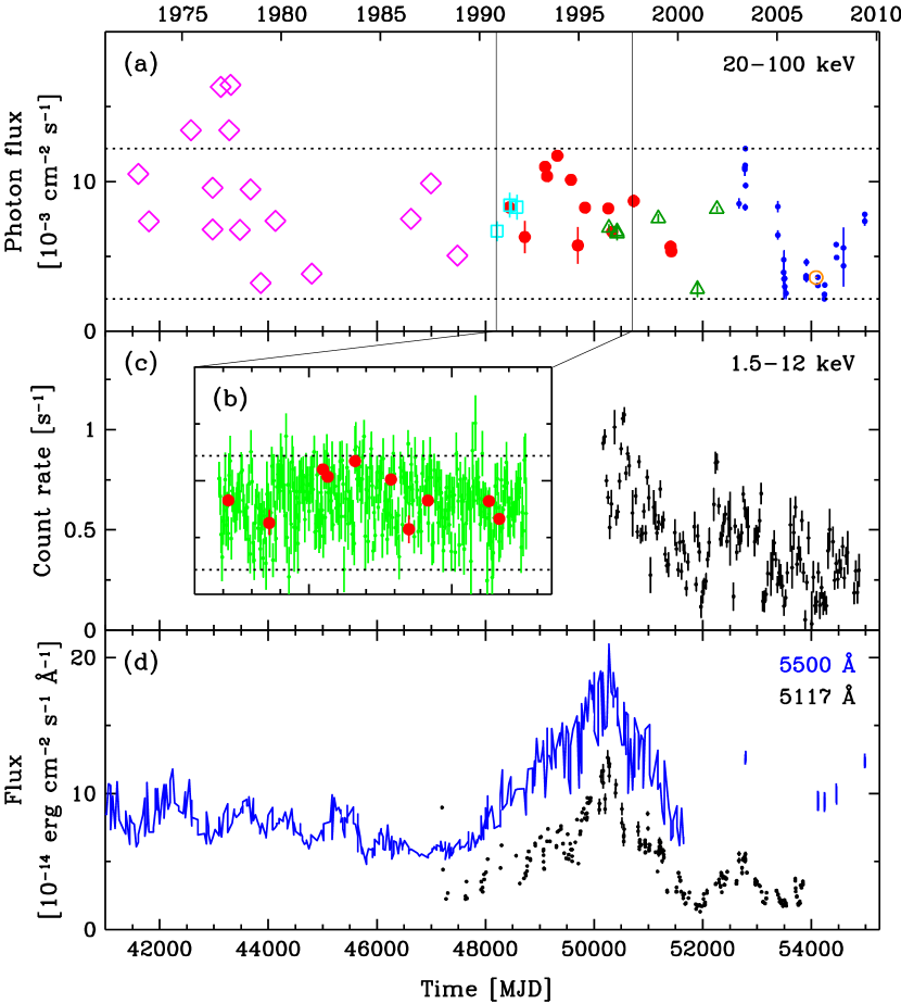
Figure 1: Light curves of NGC 4151 since 1972. (a) The 20–100 keV flux from the compilation by Perotti et al. (1991), magenta diamonds, and from GRANAT/SIGMA (cyan squares), CGRO/OSSE (red filled circles), BeppoSAX/PDS (green triangles), INTEGRAL/ISGRI (blue dots), and Suzaku/PIN (the orange open circle). The dotted lines show the extrema of the 20–100 keV flux from ISGRI. (b) The 20–100 keV flux from CGRO/BATSE (green error bars) together with that from OSSE (red filled circles; same as in a). (c) The RXTE/ASM count rate in 30-d bins. (d) The 5500 Å flux (Czerny et al. 2003, blue lines), and from INTEGRAL/OMC (vertical blue bars at MJD $>52000$), and the 5117 Å flux (Shapovalova et al. 2008, black dots).

The 1.5–12 keV count rate appears well correlated with the optical fluxes, see Fig. 1. As found by Czerny et al. (2003), the medium-energy X-ray flux of NGC 4151 varies on time scales $\sim 5$–$10^{3}$ d, whereas the optical variability is also present on longer time scales. For hard X-rays, a correlation with the optical and the 1.5–12 keV fluxes is less clear. The main peak of the optical emission at MJD $\simeq 49000$–51000 (1993–1998) is reflected in the 1.5–12 keV flux but not in the 20–100 keV one (including the BATSE data). The later data from BeppoSAX, INTEGRAL and Suzaku show an overall agreement with the optical and softer X-ray fluxes in a sense that the minima at MJD $\sim$52000 and MJD $\sim$54000 and the maximum at MJD $\sim$52800 appear for all these bands. However, the scarce hard X-ray coverage prevents unambiguous conclusions.

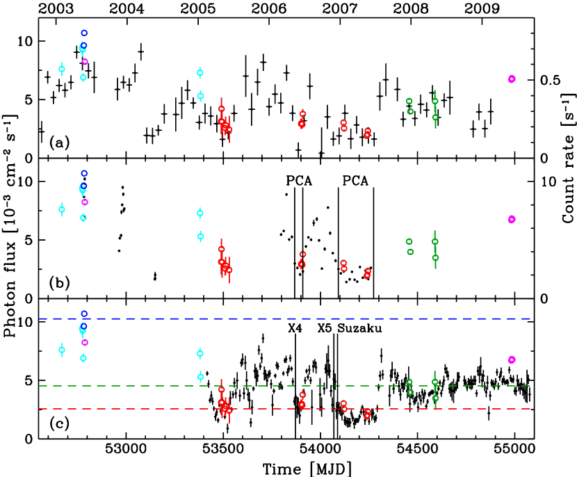
Figure 2: Medium and hard X-ray light curves from INTEGRAL/ISGRI compared to those from RXTE and Swift (shown with black circles and error bars). The 18–50 keV ISGRI flux is shown by open circles on all panels. The colours identify the three main states, bright (blue), medium (green), dim (red) and, additionally, data excluded from the spectral analysis, Revs. 0076 and 0809–0811 (magenta), and the rest (cyan). (a) The RXTE/ASM count rate in 30-d bins (right axis). (b) The RXTE/PCU2 count rate (right axis). The vertical lines delineate the two periods for which the dim state PCA spectrum was obtained. (c) Comparison with the Swift/BAT 15–50 keV flux in 7-d bins. The vertical lines show the times of the X4 (dim), X5 (medium) XMM-Newton observations and that of Suzaku (dim). The horizontal dashed lines show the average flux levels of ISGRI bright, medium and dim states.

The results shown in Fig. 1(a–b) show that the hard X-ray emission of NGC 4151 has varied in well defined limits over the last 39 years. Almost all fluxes are within the extreme 20–100 keV fluxes from ISGRI (with the maximum in 2003 May and the minimum in 2007 May). There are four flux measurements from older (1975–77) observations above this maximum. However, they are relatively doubtful, corresponding to marginal ($\approx 2$–$3\sigma$) detections at $\ga$ 40 keV. Thus, ISGRI 20–100 keV flux range appears very close to the corresponding overall actual range. This is also supported by the BATSE data, Fig. 1(b), varying within this range. We also notice that NGC 4151 was rarely seen at low hard X-ray fluxes before the INTEGRAL launch.

Fig. 2 compares ISGRI 18–50 keV fluxes with the contemporaneous data in the medium and hard X-ray bands from RXTE and Swift. The ISGRI fluxes are well correlated with those from both RXTE and the Swift/BAT. In particular, we see a good correlation with the 1.5–12 keV rate in spite of the variable absorption affecting a lower part of this band. Fig. 2 also shows that a large fraction of the INTEGRAL observations happened during periods with very low hard X-ray flux. Fig. 2 also identifies the INTEGRAL observations used for the spectral sets (Table 1).

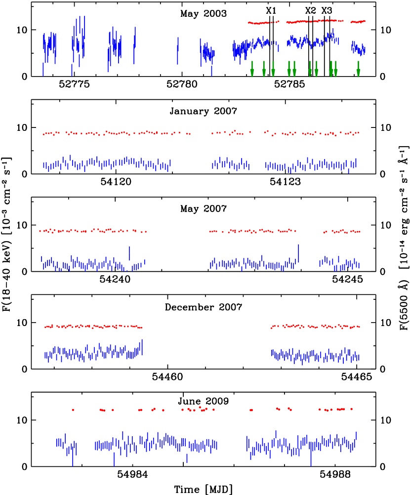
Figure 3: Illustration of short time-scale variability. The blue bars (left axis) and the red dots show the 18–40 keV ISGRI flux and the optical OMC flux, respectively, during the dedicated INTEGRAL observations. The vertical lines and the green arrows in the top panel show the times of the bright-state X1–X3 XMM-Newton and 11 RXTE/PCA observations, respectively. The data used for the bright INTEGRAL spectrum are those in the top panel simultaneous with the OMC observations except those around MJD 52788 (Rev. 0076), which have markedly lower fluxes.

The BAT light curve, Fig. 2(c), shows that the hard X-ray flux varies by a factor of a few on a week-time scale. When the source is sufficiently bright, it is possible for ISGRI to monitor hour time-scale variability. This was the case for the bright state of 2003 May, and the source showed such variability, see Fig. 3. The shown ISGRI and OMC light curves were extracted with a time bin equal to a single pointing duration (10 m–2.5 h, typically $\sim 1$ h). When observed in dimmer states, ISGRI flux remains constant within the measurement errors during a given continuous observation. The optical flux appears constant on hour–day time scales. Still, it varies on longer time scales, and it increases by $\sim$30 per cent when the source is bright in X-rays (2003 May, 2009 June).

We have extracted the bright (X1–X3) XMM-Newton/EPIC pn light curves in several energy bands in 100-s time bins, and compared with the OMC 100-s light curves. No variability is seen in either light curves on time scales $\la 1$ h. The XMM-Newton light curves vary slowly in good agreement with the trends observed for ISGRI (and also JEM-X) fluxes.

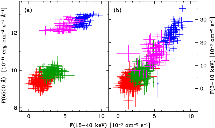
Figure 4: (a) The OMC 5500 Å flux vs. the ISGRI 18–40 keV flux. (b) The JEM-X 3–10 keV flux vs. the ISGRI flux. Each cross corresponds to a single INTEGRAL pointing. The colours identify the three main states, bright (blue), medium (green), dim (red), and, additionally, Revs. 0076, 0809–0811 (magenta).

The INTEGRAL data are suitable for correlation studies because they provide simultaneous data in the optical, medium and hard X-ray bands. Here, we use all the observations with the off-axis angle $<3\degr$ for which OMC and JEM-X data are available. They include also part of the observations not used in our spectral analysis, namely those identified with magenta circles in Fig. 2. Fig. 4 shows the correlations between the 18–40 keV flux and those fluxes in the 3–10 keV and V bands. Both show strong correlations, but the correlation patterns are different. The optical fluxes fall into two separate regions, within each they are correlated with the hard X-rays. Significant rank-order probabilities ($>\!0.999$) of the ISGRI/OMC correlation are found separately for each of the regions, but also and for the entire data set. The observed bimodality may result from strong optical long-term variability between the X-ray observations. On the other hand, the 3–10 keV and 18–40 keV fluxes exhibit a single, extremely strong, linear correlation. Statistical uncertainty blurs somewhat the correlation for low fluxes. This result indicates that during all INTEGRAL observations the slope of the X-ray spectrum of NGC 4151 below 40 keV remains approximately constant.

4 Spectral analysis

4.1 Assumptions and selection of spectral sets

Spectral fitting is performed with xspec 11.3 (Arnaud, 1996). Errors are given for 90 per cent confidence level for a single parameter, $\Delta\chi^{2}=2.7$. The luminosity and distance, $D=13.2$ Mpc, are for $H_{0}=75$ km s^-1 Mpc^-1. We use the elemental abundances of Anders & Ebihara (1982) and the photoelectric absorption cross-sections from Bałucińska-Church & McCammon (1992). The Galactic column density is set to $N_{\rm H}^{\rm G}=2.1\times 10^{20}$ cm^-2. The assumed inclination angle of the reflector and the hot plasma (for anisotropic geometries) is $i=45\degr$ (Das et al., 2005). The reflector is assumed to be neutral, and relativistic broadening of reflected spectra is neglected. Still, in some cases we test for the effects of either a variable Fe abundance of the intrinsic absorber and the reflector, a variable $i$, or an ionization of the reflector.

The main assumption used in our selection of spectral sets is that the state of the emitting hot plasma is determined by the hard X-ray flux. This is justified by our finding that the shape of ISGRI spectra for a given revolution is almost constant at a given hard X-ray flux. As an additional constraint, we do not split INTEGRAL data from a single revolution into different spectral sets. Based on this criterion, we select three average ISGRI spectra, as specified in Table 1 and Fig. 2. These spectra are accompanied by spectra taken with the other instruments. The state is assigned to each of them on the basis of the light curves presented in Figs. 2–3. In particular, the high quality of the Swift/BAT data allows us to determine the hard X-ray flux for periods with no INTEGRAL observations, and thus to assign the correct state to the existing lower-energy data sets (Table 2). On the other hand, the data from RXTE determine by themselves the hard X-ray state.

The ISGRI bright (B) and dim (D) spectra are of relatively good quality, and correspond to the extrema of the measured hard X-ray flux. For the flux range in-between, we identify two flux ranges. However, we had no corresponding low-energy data sets for the upper of them. Thus, we use the lower of them, denoted as medium (M). The fitted data sets are as follows.

The bright state, B. We use the data from 2003 May made at low off-axis angles, as shown in the top panel of Fig. 3. The spectrum includes a part of Rev. 0074 (without its beginning) and Rev. 0075. For these data, we have simultaneous RXTE and XMM-Newton observations, see Table 2. The fitted spectral set consists of ISGRI spectrum, the X1+X2 and X3 XMM-Newton spectra, and the RXTE PCU2 spectrum summed over 11 observations.

The medium state, M. We sum ISGRI data from Revs. 0634, 0636, 0678–0679, and use the summed JEM-X 1 spectrum from Revs. 0634 and 0636, and the X5 XMM-Newton spectrum.

The dim state, D. The summed ISGRI spectrum is from Revs. 0310–0563. We use the RXTE PCU2, the X4 XMM-Newton EPIC pn, and the Suzaku XIS0,3 and XIS1 spectra.

We have also investigated the effect of including other available spectra for each of the data set, whose resulting sets we denote ’extended’. The extended set B also includes the spectra from the INTEGRAL/JEM-X 2 and SPI, and the RXTE/HEXTE clusters 0, 1. The extended set M also includes the SPI spectrum. The extended data set D also includes two INTEGRAL JEM-X 1 summed spectra, from Revs. 0521–0522 and 0561–0563, the Suzaku PIN spectrum, the RXTE HEXTE cluster 1 spectrum, and the corresponding SPI spectrum. We discuss the effect of using the extended data sets in Section 4.3 below.

In order to limit the complexity of the fitted models, we have decided not to use the X-ray spectra at $E<2.5$ keV. A two-component partial absorption was then sufficient to model absorption of the continuum. Using the X-ray spectra in the 0.1–2.5 keV band would have required to add a number of spectral lines as well as a soft excess component. As we have tested, including that low-energy band would not affect our determination of the parameters of the hot plasma and of Compton reflection.

Thus, the EPIC pn, XIS0+XIS3, and XIS1 spectra were used in the 2.5–11.3 keV, 2.5–9.5 keV and 2.5–9.0 keV bands, respectively. The PCA/PCU2 and JEM-X spectra were fitted in the 3–16 keV and 4–19 keV bands, respectively. The HXD/PIN spectrum was used in the 19–60 keV band because the $<$19-keV data were showing a strong excess. For ISGRI, data below 20 keV were always excluded, whereas the high-energy limit was in the 180–200 keV range, depending on our $3\sigma$ detection threshold used to select good spectral channels. The ISGRI spectra in the staring mode from Revs. 0074–75 show an excess of $\sim$10 per cent below 23 keV, whose origin remains unknown. It could be related to a specific setting of the low-energy threshold in the early period of the mission. Thus, we used only the data at $>23$ keV in this case. The HEXTE spectra were used in the 13–160 keV band for the bright state and in 23–110 keV for the dim state. The SPI spectra were fitted in the 23–200 keV band.

While fitting a given spectral set, the parameters of intrinsic continua are the same for all included spectral data, allowing only the normalization of the model to vary between them. This reflects our assumption that the hard X-ray flux determines the intrinsic state of the source, even for non-simultaneous data. On the other hand, absorption and the Fe K emission may vary quickly (Puccetti et al., 2007), and we cannot expect their parameters to be the same for different low-energy spectra associated with the same spectral set. Thus, we have allowed them to vary between different spectra. Our assumed absorber consists of one fully covering the source with the column density of $N_{\rm H}^{\rm i}$, and the ionization parameter, $\xi\equiv 4\pi F_{\rm i}/n$, where $F_{\rm i}$ is the 5 eV–20 keV irradiating flux and $n$ is the density of the reflector. For the low-resolution detectors, PCA and JEM-X, we assumed $\xi=0$. For the high-resolution detectors, EPIC pn and XIS, we allowed $\xi>0$, and, in addition, we included partial-covering neutral absorption, with the column density of $N_{\rm H}^{p}$ covering a fraction of $f^{\rm p}$ of the flux. For the ionized absorption, we use the model by Done et al. (1992). Although it is not applicable to highly ionized plasma, it is sufficiently accurate at low/moderate ionization, such as that found in our data. Absorption for ISGRI, HEXTE, SPI and PIN spectra is only marginally important, and we thus used only the neutral fully-covering $N_{\rm H}^{\rm i}$ at the values fitted to the corresponding PCA or JEM-X spectra. The Fe K$\alpha$ emission is modelled by a Gaussian line, with the centre energy, width, photon flux and equivalent width of $E_{\rm Fe}$, $\sigma_{\rm Fe}$, $I_{\rm Fe}$ and $w_{\rm Fe}$, respectively. Fitting the dim state spectra, we have found that adding an Fe K$\beta$ line (at $\approx$7.1 keV) was significantly improving the fit for the EPIC pn and XIS spectra.

4.2 The cut-off power-law model

We first fit an e-folded power-law model including a Compton reflection component. This allows us to compare our results to other published ones. We use the pexrav model (Magdziarz & Zdziarski, 1995), and our other assumptions are specified above. The results are shown in Table 3, where we do not show the fitted absorber and line parameters since they are similar to those for our main model of thermal Comptonization, see Section 4.3 below.

Our results regarding $\Gamma$ and $R$ are similar to those of earlier works. However, a significant difference is found for the e-folding energy, $E_{\rm c}$, which we find to be high, and compatible with no cut-off for two of our states, see Table 3. A finite $E_{\rm c}$ is found only for the bright state. Even then, we obtain values well above those reported before, which are 30–45 keV (P01), 80–180 keV (De Rosa et al., 2007) and $\sim$210 keV (Z02). As discussed in Zdziarski et al. (2003), an exponential cut-off is much shallower than that characteristic of thermal Comptonization, and not sharp enough to model the spectral high-energy cut-offs observed in Seyferts, in particular in NGC 4151. Thus, our high values of $E_{\rm c}$ result from the good quality of the data below the cut-off, which dominate the statistics and force an approximately straight power law to continue to just below the beginning of the cut-off.

Table 3: Spectral fitting results for the e-folded power-law model including reflection. The xspec model is constant*wabs*absori*zpcfabs(pexrav +zgauss), and the normalization, $K$, is given by the photon flux at 1 keV in units of $10^{-2}$ keV^-1 cm^-2 s^-1.

State	$E_{\rm c}$ [keV]	$\Gamma$	$R$	$K$	$\chi^{2}$/d.o.f.
Bright	264${}_{-26}^{+48}$	1.71${}_{-0.01}^{+0.06}$	0.45${}_{-0.05}^{+0.12}$	8.7${}_{-0.3}^{+1.1}$	3179/3414
Medium	$>$ 1025	1.81${}_{-0.03}^{+0.05}$	0.6${}_{-0.3}^{+0.3}$	4.6${}_{-0.7}^{+1.4}$	1554/1599
Dim	$>$ 1325	1.81${}_{-0.01}^{+0.01}$	0.92${}_{-0.05}^{+0.05}$	2.24${}_{-0.02}^{+0.01}$	3338/3384

4.3 Comptonization model

Table 4: (a) Spectral fitting results with thermal Comptonization as the main continuum. The xspec model is constant*wabs*absori*zpcfabs*(compps +zgauss). See Section 4.3 for the definitions of the parameters. $L_{\rm X\gamma}$ and $L_{\rm X\gamma}^{\prime}$ are the bolometric model luminosity (in units of $10^{43}$ erg s^-1) with and without the reflection component, respectively, and only the values for the geometry 0 are given as the values for other geometries are similar.

State	$kT_{\rm e}$ [keV]	$y$	$\tau$	$R$	$K\,[10^{8}]$	$L_{\rm X\gamma}$	$L_{\rm X\gamma}^{\prime}$	Geometry	$\chi^{2}$/d.o.f.
Bright	54${}_{-5}^{+7}$	1.10${}_{-0.02}^{+0.02}$	2.6${}_{-0.3}^{+0.3}$	0.40${}_{-0.06}^{+0.07}$	5.2${}_{-0.6}^{+1.4}$	5.18	4.61	sphere (0)	3165/3414
	62${}_{-7}^{+7}$	0.60${}_{-0.01}^{+0.01}$	1.3${}_{-0.1}^{+0.1}$	0.55${}_{-0.07}^{+0.08}$	7.3${}_{-0.9}^{+1.9}$			slab (1)	3166/3414
	62${}_{-7}^{+9}$	0.61${}_{-0.01}^{+0.01}$	1.3${}_{-0.2}^{+0.1}$	0.55${}_{-0.06}^{+0.09}$	3.9${}_{-0.7}^{+0.4}$			slab ($-1$)	3166/3414
	73${}_{-9}^{+14}$	1.06${}_{-0.02}^{+0.02}$	1.9${}_{-0.2}^{+0.4}$	0.47${}_{-0.07}^{+0.05}$	12.0${}_{-1.6}^{+2.9}$			cylinder (2)	3168/3414
	73${}_{-13}^{+13}$	1.06${}_{-0.01}^{+0.03}$	1.9${}_{-0.3}^{+0.3}$	0.51${}_{-0.9}^{+0.5}$	5.4${}_{-1.1}^{+1.4}$			cylinder ($-2$)	3168/3414
	73${}_{-7}^{+16}$	1.21${}_{-0.02}^{+0.02}$	2.1${}_{-0.6}^{+0.4}$	0.48${}_{-0.06}^{+0.06}$	11.9${}_{-1.4}^{+3.2}$			hemisphere (3)	3168/3414
	73${}_{-9}^{+15}$	1.21${}_{-0.02}^{+0.03}$	2.1${}_{-0.4}^{+0.3}$	0.50${}_{-0.06}^{+0.08}$	4.7${}_{-1.0}^{+1.5}$			hemisphere ($-3$)	3168/3414
	61${}_{-5}^{+7}$	0.80${}_{-0.02}^{+0.01}$	1.7${}_{-0.2}^{+0.1}$	0.38${}_{-0.05}^{+0.04}$	1.2${}_{-0.1}^{+0.1}$			sphere (4)	3172/3414
	57${}_{-7}^{+13}$	0.86${}_{-0.01}^{+0.01}$	1.9${}_{-0.4}^{+0.2}$	0.39${}_{-0.05}^{+0.06}$	6.4${}_{-0.6}^{+0.6}$			sphere ($-4$)	3169/3414
	57${}_{-5}^{+10}$	0.86${}_{-0.01}^{+0.01}$	1.9${}_{-0.3}^{+0.2}$	0.38${}_{-0.05}^{+0.06}$	4.9${}_{-0.4}^{+1.5}$			sphere ($-5$)	3166/3414
Medium	128${}_{-24}^{+74}$	1.02${}_{-0.13}^{+0.08}$	$1.0_{-0.3}^{+0.5}$	$<0.41$	3.9${}_{-1.0}^{+0.4}$	2.26	2.16	sphere (0)	1554/1597
Dim	190${}_{-12}^{+13}$	0.98${}_{-0.01}^{+0.01}$	0.66${}_{-0.05}^{+0.04}$	0.75${}_{-0.04}^{+0.04}$	1.54${}_{-0.01}^{+0.01}$	1.47	1.19	sphere (0)	3337/3384
	200${}_{-8}^{+7}$	0.49${}_{-0.01}^{+0.01}$	0.31${}_{-0.01}^{+0.01}$	1.01${}_{-0.05}^{+0.05}$	2.04${}_{-0.02}^{+0.01}$			slab (1)	3335/3384
	188${}_{-7}^{+6}$	0.48${}_{-0.01}^{+0.01}$	0.33${}_{-0.01}^{+0.01}$	1.04${}_{-0.05}^{+0.05}$	1.20${}_{-0.01}^{+0.01}$			slab ($-1$)	3350/3384
	210${}_{-14}^{+12}$	1.05${}_{-0.01}^{+0.01}$	0.64${}_{-0.04}^{+0.04}$	0.79${}_{-0.04}^{+0.04}$	2.85${}_{-0.01}^{+0.02}$			cylinder (2)	3334/3384
	215${}_{-13}^{+12}$	1.01${}_{-0.01}^{+0.01}$	0.60${}_{-0.03}^{+0.04}$	0.86${}_{-0.05}^{+0.05}$	1.73${}_{-0.01}^{+0.01}$			cylinder ($-2$)	3336/3384
	227${}_{-14}^{+10}$	1.21${}_{-0.02}^{+0.01}$	0.68${}_{-0.03}^{+0.04}$	0.84${}_{-0.04}^{+0.04}$	2.89${}_{-0.02}^{+0.01}$			hemisphere (3)	3334/3384
	220${}_{-11}^{+13}$	1.14${}_{-0.01}^{+0.01}$	0.66${}_{-0.04}^{+0.03}$	0.90${}_{-0.05}^{+0.05}$	1.71${}_{-0.01}^{+0.02}$			hemisphere ($-3$)	3336/3384
	186${}_{-9}^{+11}$	0.66${}_{-0.01}^{+0.01}$	0.45${}_{-0.03}^{+0.02}$	0.77${}_{-0.04}^{+0.04}$	0.866${}_{-0.004}^{+0.004}$			sphere (4)	3341/3384
	191${}_{-17}^{+13}$	0.86${}_{-0.01}^{+0.01}$	0.58${}_{-0.04}^{+0.05}$	0.77${}_{-0.04}^{+0.04}$	1.56${}_{-0.01}^{+0.01}$			sphere ($-4$)	3337/3384
	196${}_{-13}^{+13}$	0.81${}_{-0.01}^{+0.01}$	0.53${}_{-0.04}^{+0.04}$	0.77${}_{-0.04}^{+0.04}$	1.49${}_{-0.01}^{+0.01}$			sphere ($-5$)	3337/3384

Table 4: (b) Continuation of Table 4(a). Fit results with the thermal Comptonization model (for a sphere, the geometry parameter $=0$) regarding the absorber, line component, and the relative normalization, $C_{\rm ISGRI}$, of a given X-ray spectrum with respect to ISGRI. See Section 4.1 for the definitions of the other parameters. The units of $N_{\rm H}$, $\xi$, and $I_{\rm Fe}$ are $10^{22}$ cm^-2, $10^{-2}$ erg cm s^-1, $10^{-4}$ cm^-2 s^-1, respectively, and ‘f’ denotes a fixed parameter.

State	X-ray spectrum	$C_{\rm ISGRI}$	$N_{\rm H}^{\rm i}$	$\xi$	$N_{\rm H}^{\rm p}$	$f^{\rm p}$	$E_{\rm Fe}$ [keV]	$\sigma_{\rm Fe}$ [keV]	$I_{\rm Fe}$	$w_{\rm Fe}$ [eV]
Bright	EPIC pn (X1+X2)	0.92${}_{-0.03}^{+0.03}$	4.9${}_{-0.7}^{+0.9}$	10${}_{-6}^{+79}$	15.8${}_{-3.3}^{+3.9}$	0.39${}_{-0.07}^{+0.09}$	6.400${}_{-0.011}^{+0.011}$	0.07${}_{-0.01}^{+0.02}$	3.0${}_{-0.3}^{+0.3}$	83${}_{{{-9}}}^{{{+7}}}$
	EPIC pn (X3)	1.08${}_{-0.03}^{+0.03}$	3.0${}_{-1.8}^{+1.5}$	64${}_{-61}^{+47}$	9.5${}_{-1.1}^{+4.0}$	0.55${}_{-0.22}^{+0.18}$	6.393${}_{-0.012}^{+0.013}$	0.07${}_{-0.01}^{+0.01}$	2.8${}_{-0.3}^{+0.3}$	76${}_{{{-9}}}^{{{+9}}}$
	PCA PCU2 (B)	1.17${}_{-0.03}^{+0.03}$	7.4${}_{-0.4}^{+0.4}$	0f	0f	–	6.06${}_{-0.09}^{+0.08}$	0.36${}_{-0.13}^{+0.15}$	6.8${}_{-0.8}^{+1.3}$	169${}_{{{-20}}}^{{{+32}}}$
Medium	EPIC pn (X5)	0.83${}_{-0.06}^{+0.08}$	7.6${}_{-0.4}^{+0.5}$	4${}_{-3}^{+11}$	22.6${}_{-1.5}^{+4.4}$	0.50${}_{-0.04}^{+0.05}$	6.388${}_{-0.007}^{+0.007}$	0.06${}_{-0.01}^{+0.01}$	2.7${}_{-0.3}^{+0.5}$	149${}_{{{-12}}}^{{{+27}}}$
	JEM-X (M)	0.74${}_{-0.06}^{+0.06}$	13.0${}_{-3.3}^{+3.7}$	0f	0f	–	–	–	–	–
Dim	EPIC pn (X4)	1.17${}_{-0.01}^{+0.01}$	6.36${}_{-0.15}^{+0.14}$	4${}_{-3}^{+30}$	23.5${}_{-0.7}^{+0.6}$	0.69${}_{-0.01}^{+0.01}$	6.398${}_{-0.005}^{+0.004}$	0.06${}_{-0.01}^{+0.01}$	2.3${}_{-0.1}^{+0.1}$	271${}_{{{-13}}}^{{{+13}}}$
	XIS0,3 (D)	1.11${}_{-0.01}^{+0.01}$	8.03${}_{-0.16}^{+0.12}$	0.7${}_{-0.4}^{+0.9}$	28.8${}_{-1.0}^{+0.9}$	0.50${}_{-0.01}^{+0.01}$	6.384${}_{-0.003}^{+0.003}$	0.03${}_{-0.01}^{+0.01}$	2.2${}_{-0.1}^{+0.1}$	291${}_{{{-13}}}^{{{+13}}}$
	XIS1 (D)	1.13${}_{-0.01}^{+0.01}$	fitted together with XIS0,3				6.412${}_{-0.004}^{+0.005}$	0.04${}_{-0.01}^{+0.01}$	2.3${}_{-0.1}^{+0.1}$	280${}_{{{-13}}}^{{{+13}}}$
	PCA PCU2 (D)	1.16${}_{-0.01}^{+0.01}$	13.6${}_{-0.5}^{+0.5}$	0f	0f	–	6.4f	0f	2.1${}_{-0.3}^{+0.3}$	303${}_{{{-39}}}^{{{+39}}}$

To model thermal Comptonization, we use the compps model (Poutanen & Svensson, 1996) in xspec. It models Compton scattering in a plasma cloud of given temperature, $T_{\rm e}$, and Thomson optical depth, $\tau$, for a number of geometries and locations of the seed photon sources. Since $T_{\rm e}$ and $\tau$ are strongly intrinsically anticorrelated, we also use the Compton parameter (e.g., Rybicki & Lightman 1979), $y\equiv 4(kT_{\rm e}/m_{\rm e}c^{2})\tau$ (where $m_{\rm e}$ is the electron mass) as the second fitting parameter instead of $\tau$. The advantage of this choice is that $T_{\rm e}$ and $y$ are almost orthogonal; $y$ determines closely the power-law slope at low energies whereas $kT_{\rm e}$ determines the position of the high-energy cut-off. The seed photons are assumed to have a disc blackbody distribution (diskbb in xspec, Mitsuda et al. 2004) with the maximum temperature of $kT_{\rm bb}=10$ eV. The model normalization, $K$, is that of the seed disc blackbody model as defined in xspec, see Section 5.3.

Among the geometries included in compps, we consider here four spherical cases; an approximate treatment of radiative transfer using escape probability (which is denoted in compps by the geometry parameter $=0$), a sphere with central soft photons (geometry 4), homogeneously distributed seed photons (geometry $-4$) and seed photons distributed according to the diffusion-equation eigen-function, $\propto\sin(\pi\tau^{\prime}/\tau)/(\pi\tau^{\prime}/\tau)$, where $0\leq\tau^{\prime}\leq\tau$ ($-5$). Then, we consider a slab with the seed photons either at its bottom (geometry 1) or distributed homogeneously (geometry $-1$). Also, we consider the hot plasma in the shape of either a cylinder with the height equal to its radius, or a hemisphere, with the seed photons being either at its bottom (2, 3, respectively) or homogeneously distributed ($-2$, $-3$, respectively).

The spectral data of NGC 4151 studied in this paper are of high quality and represent the largest set ever collected for this source. This gives us a possibility to test how precise information about X$\gamma$ emission from brightest Seyferts can be achieved with the current satellites. Therefore, we extensively test various variants of the Comptonization model for our two best-quality states, bright and dim. This could, in principle, give us some indications regarding the actual geometry of the source. Our results are presented in Tables 4(a) and (b), regarding the parameters of the Comptonizing plasma and the strength of reflection (which are the same for all used detectors within a given state), and of the absorber and the Fe line (which are specific to a given X-ray detector within each of the states), respectively. The results in Table 4(b) and the entries for the bolometric model luminosity, $L_{\rm X\gamma}$, in Table 4(a) are given only for the case of spherical geometry calculated using escape probability formalism (geometry 0).

We find the thermal Comptonization model to provide very good fits to the data. The values of the reduced $\chi^{2}$ are $\la 1$, which, however, appears not to be due to an overly complex model. In particular, the high-energy continua are determined only by three parameters, $y$, $R$, $kT_{\rm e}$. For the bright state, Comptonization provides a much better fit than the e-folded power law, with $\Delta\chi^{2}$ of up to $-14$. However, any trends seen for the geometry of the Comptonizing plasma are rather weak. In the case of the bright state, equally good models can be obtained with either a slab or a sphere. Also, models with seed photons being distributed within the source are of similar quality as those with localized seed photons. On the other hand, the differences between the models are slightly stronger in the case of the dim state. In particular, the slab model with seed photons at its bottom is somewhat better than that with the seed photons distributed throughout it. This can be a hint that the actual source has the seed photons external to the source rather than internal (which would be the case for the dominant synchrotron seed photons). We also note that the fitted values of $kT_{\rm e}$ are rather insensitive to the assumed geometry in both the bright and dim states. Our results for the bright state are similar to those of previous Comptonization fits, in particular to those of Z02, who obtained $kT_{\rm e}=73^{+34}_{-29}$ keV, $y=0.88^{+0.12}_{-0.11}$, and $R=0.60^{+0.24}_{-0.21}$ at $L_{\rm X\gamma}\simeq 3.9\times 10^{43}$ erg s^-1 using a broad-band X-ray spectrum from ASCA and OSSE.

In all geometries, we see in Table 4(a) that the Compton $y$ parameter remains approximately constant between the bright and dim states, with only a slight decrease in the dim state. For the medium state, Table 4(a) gives the results only for the model with escape probabilities, for which the best fit $y$ is almost the same as that in the dim state. These results are illustrated by the confidence contours shown in Fig. 5.

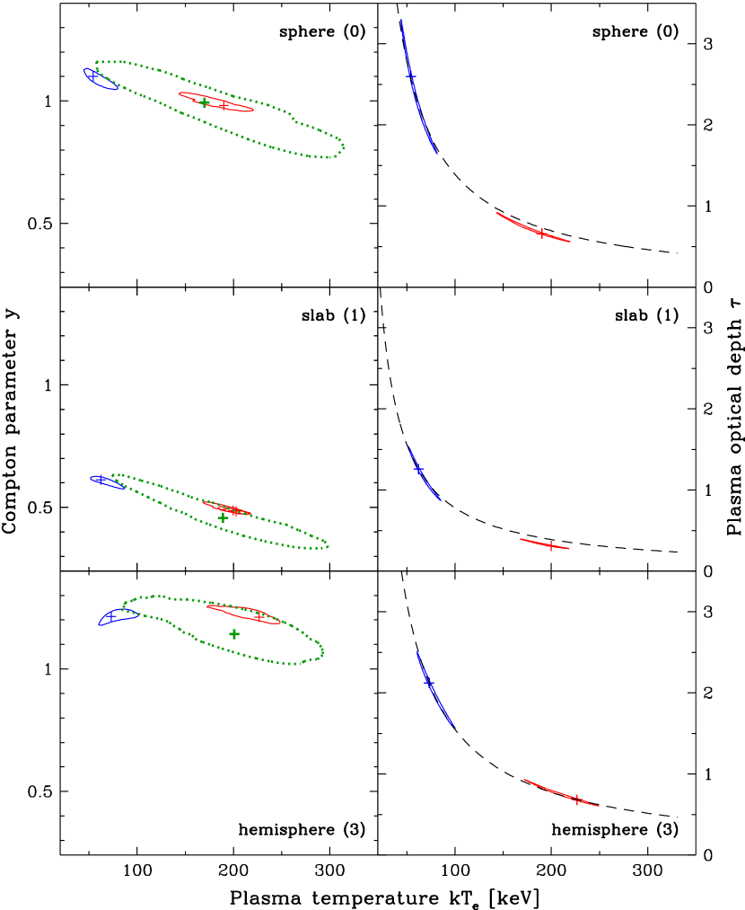
Figure 5: The 90 per cent confidence regions for the Compton $y$ parameter (left) and the optical depth, $\tau$ (right), vs. the temperature, $kT_{\rm e}$ for three geometries of the Comptonizing plasma. The solid blue, solid red and green dashed (only for $y$) contours correspond to the bright, dim and medium state, respectively. The dashed curves for $\tau$ vs. $kT_{\rm e}$ correspond to $\tau\propto kT_{\rm e}^{-1}$, normalized to the bright-state results.

Apart from the results given in Table 4, a reduction of $\chi^{2}$ appears when the Fe abundance (assumed equal for the absorber and the reflector) is a free parameter. We found a moderate overabundance, ${1.5\pm 0.2}$ times that of Anders & Ebihara (1982) for the bright state, with $\Delta\chi^{2}=-6$, and ${1.3\pm 0.1}$ for the dim state, $\Delta\chi^{2}=-2$. For the XMM-Newton observation in 2000 December, an Fe overabundance by 2–3 was claimed by Schurch et al. (2003) but that fit was done with the XMM-Newton spectrum only and the reflection strength (affecting that determination) was not well constrained.

We also find that both the bright and dim state spectra prefer an inclination angle $>45\degr$, with $\Delta\chi^{2}=-3$ and $-6$, respectively, at $75\degr$. Since this effect is observed for symmetric (sphere) and asymmetric (hemisphere) geometries, we conclude that its main cause is the changing shape of the reflection component. On the other hand, allowing the reflector to be ionized does not improve the fit, and $\xi<0.2$ erg cm s^-1 (at an assumed reflector temperature of $10^{5}$ K).

The lack of the far-UV and very soft X-ray spectra does not allow us to fit the maximum temperature of the seed disc blackbody photons, $kT_{\rm bb}$. We have found that changing it to either 5 or 20 eV yields no improvement of the fit. This is indeed expected given that the photon energies emitted by the disc are much below the fitted energy range, at which the shape of the Comptonization spectrum has already achieved a power-law shape independent of $kT_{\rm bb}$.

Table 4(b) also shows the normalization of a given X-ray spectrum relative to that from ISGRI. For the bright state, when the INTEGRAL, XMM-Newton and RXTE observations were almost contemporary, $C_{\rm ISGRI}$ is very close to 1 and, for both of the XMM-Newton spectra, it follows the flux changes seen in the top panel of Fig. 3. This shows that ISGRI, EPIC pn and PCA detectors are well cross-calibrated. In the case of the two other spectral sets, the observations are not simultaneous. Nevertheless, $C_{\rm ISGRI}$ varies only within the range of 0.74–1.17, confirming the validity of our selection of the spectra for a given flux state.

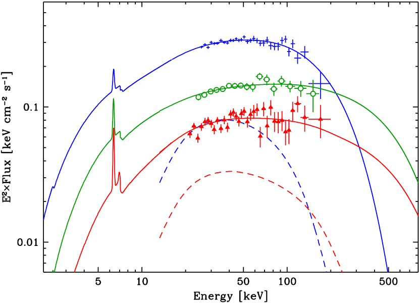
Figure 6: The Comptonization model spectra (solid curves; the geometry parameter $=0$) of the three states of the NGC 4151, shown together with ISGRI spectra. The bright, medium and dim spectra are shown by the blue crosses, green circles and red triangles, respectively. The dashed curves show the reflection model components for the bright (upper) and dim state. The fitted JEM-X, RXTE, XMM-Newton and Suzaku spectra are not shown for clarity.

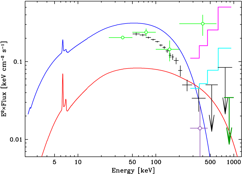
Figure 7: The Comptonization models for the extreme states (solid curves, same as in Fig. 6) compared to the average OSSE spectrum (crosses and two $2\sigma$ upper limits). The rightmost upper limit is the COMPTEL upper limit in the 0.75–1 MeV band (Maisack et al., 1995). The histograms give the INTEGRAL/PICsIT $3\sigma$ upper limits for 1 Ms (upper) and 10 Ms (lower) effective exposure time. The PICsIT 1.34 Ms average 277–461 keV flux is shown by error bars with a diamond. The SPI spectrum obtained by Bouchet et al. (2008) is shown by error bars with circles. Note that the 200–600 keV data point may be spurious.

We have also tested our results using the extended data sets (see Section 4.1). However, the quality of the fits and the plasma parameter uncertainty are not improved when they are used. This confirms that our selection of the primary sets was valid. Thus, we do not present here those results.

We note that even for such a bright AGN as NGC 4151, we have no data at energies $\ga 200$ keV, as shown in Fig. 6. Still, for the dim state, we have found $kT_{\rm e}\simeq 200$ keV with a statistical uncertainty of $\sim 7$ per cent or so. The physical reason for this low uncertainty is the observed lack of spectral curvature. In the process of thermal Comptonization, a power law slope at $E\la kT_{\rm e}$ appears due to the merging of many individual up-scattering profiles, each being curved. The cut-off at $E\ga kT_{\rm e}$ is due to the electron energies being comparable to the photon ones, in which case a photon no longer increases its energy in a scattering. Since we see no cut-off up to $\sim$200 keV, models with a lower $kT_{\rm e}$ are ruled out. On the other hand, models with a higher $kT_{\rm e}$ correspond to an increase of the photon energy in a single scattering by a factor so large that the individual, curved, scattering profiles become clearly visible and the spectrum at $E\la kT_{\rm e}$ is no longer a power law. Since the observed spectral shape is a power law, this case is also excluded. We note, however, that our assumed model corresponds to a single scattering zone. A power law spectrum at $E\la 200$ keV may also be produced by a superposition of emission regions with different temperatures (smoothing out the resulting spectrum), as, e.g., in a hot accretion flow. In this case, the maximum temperature of the flow could be higher than 200 keV. In any case, we do see a very clear difference in the characteristic Comptonization temperature between the bright and dim state.

We comment here on the very high value of $kT_{\rm e}=315\pm 15$ keV obtained by P01 for the 1999 January BeppoSAX spectrum of NGC 4151. The fit of that model appears rather poor when compared with the curvature of the BeppoSAX/PDS data above 50 keV, see fig. 2(b) in P01. We also find that the PDS spectrum is very similar to the average OSSE spectrum (Johnson et al., 1997), shown in Fig. 7 (with only the normalization of the PDS spectrum being about 5 per cent lower). This indicates that the source was in a moderately bright state in 1999 January, for which state the temperature of 315 keV appears highly unlikely. We cannot explain this discrepancy; it may be that $kT_{\rm e}=315\pm 15$ keV represented a spurious local minimum.

As we see in Fig. 7, our bright-state model spectrum agrees well in shape with the average OSSE spectrum (Johnson et al., 1997). The latter also agrees with the first three points of the average NGC 4151 spectrum from INTEGRAL/SPI (Bouchet et al., 2008). However, the SPI 200–600 keV flux is implausibly high, which may reflect a problem with the background estimate. Indeed, the SPI analysis of Petry et al. (2009) yields only upper limits at $E>150$ keV.

We see in Fig. 7 that the Comptonization models of the bright and dim states cross at $\simeq 300$ keV. Unfortunately, it is impossible to verify it with our data. In particular, we cannot test if there is any non-thermal component at high energy. Even the average spectrum from OSSE, the most sensitive detector up to date at $E\ga 150$ keV, gives only a weak detection of NGC 4151 at $E\ga 250$ keV with an $>4$ Ms exposure time. From the shown upper limits (including systematic errors) of the INTEGRAL/PICsIT, the current detector most sensitive at $E\ga 250$ keV (Lubiński, 2009), we see it would need $>10$ Ms exposure time to detect NGC 4151 in the 300–400 keV range. Merging all the suitable INTEGRAL data (with the effective exposure time of 1.34 Ms taken without the bright state, for which the observation was in the staring mode, not suitable for the PICsIT), we extracted the PICsIT flux in the 277–461 keV band. Although it is not a detection (and the shown error bar does not include systematic errors), it provides a hint that the average NGC 4151 emission in this energy range is weak.

5 Discussion

5.1 Reflection and Fe line

5.1.1 Comparison with previous work

A reflection component in the X-ray spectra of NGC 4151 was first found by Zdziarski et al. (1996a), using contemporaneous data from CGRO and Ginga, yielding $R\simeq 0.43$ (using a Comptonization model and assuming $i=65\degr$). Then, Z02 found $R\simeq 0.6$ (at $i=17\degr$) using CGRO and ASCA data, and P01 found $R\simeq 0.2$–1.8 using BeppoSAX data and a reflection model averaged over the viewing angle. A previous analysis of INTEGRAL bright-state data from 2003 May yielded a larger reflection, $R=0.72\pm 0.14$ (Beckmann et al., 2005), than that determined by us (their value of $kT_{\rm e}=94_{-10}^{+4}$ keV is also different from that found by us for the same data). By fitting the ISGRI and JEM-X bright-state spectra alone, we find results very similar to those with the XMM-Newton and RXTE spectra included (Table 4). Therefore the differences appear to be a consequence of the substantial change of the INTEGRAL calibration since 2005. Furthermore, Beckmann et al. (2005) used the SPI spectra obtained in the staring observation mode, which can be affected by a large background uncertainty. Then, De Rosa et al. (2007) found $R\simeq 0.4$ for several BeppoSAX spectra and $R\simeq 0$ for the remaining ones, but using an e-folded power-law model rather than Comptonization. Then, Schurch & Warwick (2002) found $R\simeq 1.9$ using XMM-Newton data assuming $i=65\degr$, but this result was obtained using the 2.5–12 keV band only and assuming a fixed $\Gamma=1.65$.

Regarding Fe K$\alpha$ line, Zdziarski et al. (1996a) found a narrow line with $I_{\rm Fe}\simeq(0.6$–$1.0)\times 10^{-4}$ cm^-2 s^-1 using Ginga data, and Z02 found a narrow line at $I_{\rm Fe}\simeq 2.5\times 10^{-4}$ cm^-2 s^-1 accompanied by a weaker broad relativistic line using ASCA data. The broad component has not been observed later, whereas the narrow line flux measured by BeppoSAX (De Rosa et al., 2007), Chandra (Ogle et al., 2000) and XMM-Newton (Schurch et al., 2003) was found to be in the range (1.3–$4.2)\times 10^{-4}$ cm^-2 s^-1. As seen in Tables 4(a–b), our results on $R$ and $I_{\rm Fe}$ approximately agree with the previous measurements.

5.1.2 Close and distant reflector

We see in Table 4(a) that the relative strength of reflection, $R$, is close to being twice higher in the dim state than in the bright one. (In the medium state, the amount of data is very limited, and the apparent lack of detectable reflection may be not typical to that flux level.) The increase of $R$ with decreasing flux could be a real change of the solid angle subtended by the reflector between the states. On the other hand, it could be that it is due to the contribution of a distant reflector, in particular a molecular torus, as postulated in the AGN unified model. Reflection from distant media is indeed commonly seen in Seyferts 2, e.g., Reynolds et al. (1994). If we attribute the increase of $R$ in the dim state due to that component, we can calculate the fractional reflection strength from the close reflector, presumably an accretion disc, and the flux reflected from the torus, which, due to its large size, is averaged over a long time scale, and thus assumed to be the same in either state.

The hypothesis of the stable geometry of the source is supported by the approximate constancy of the Compton $y$ parameter, see Table 4(a) and Fig. 5, and of the photon index, $\Gamma$, see Table 3. Those parameters are closely related to the amplification factor of Comptonization (e.g., Beloborodov 1999), whose constancy can be most readily achieved if the system geometry is constant (e.g., Haardt & Maraschi 1991; Zdziarski et al. 1999). Thus, we consider an approximately constant relative reflection strength from the disc very likely. Observationally, we do see a strong $R$-$\Gamma$ correlation in Seyferts and X-ray binaries, which can be interpreted by a geometrical feedback model (Zdziarski et al., 1999), and which would require a constant disc $R$ for a given $\Gamma$.

The unabsorbed flux in a given state, $F_{\rm S}$, where ${\rm S}=$ either D (dim) or B (bright), is the sum of the (unabsorbed) incident (i) and reflected (r) fluxes,

$$F_{\rm S}=F_{\rm i,S}+F_{\rm r,S},$$ (1)

where $F_{\rm S}$ and $F_{\rm r,S}$ can be calculated from the results of our spectral fitting in Section 4.3. We assume that the observed (unabsorbed) reflected flux in each state is the sum of the close disc (d) state-dependent component and the constant distant torus (t) component,

$$F_{\rm r,S}=F_{\rm d,S}+F_{\rm t}.$$ (2)

Then, assuming the constancy of the solid angle subtended by the disc reflector, or, equivalently, its reflection strength, $R_{\rm d}$, the disc-reflected fluxes are,

$$F_{\rm d,S}=F_{\rm r,S}(R_{\rm d}/R_{\rm S}),$$ (3)

where $R_{\rm S}$ is the reflection strength for a given state. We have four equations (2–3) for four unknowns, $F_{\rm d,B}$, $F_{\rm d,D}$, $R_{\rm d}$ and $F_{\rm t}$, which can be readily solved. We note that they can be formulated without involving $F_{\rm i,S}$, which implies that the solution does not depend on the choice of the energy interval in which the fluxes are measured as long as it includes the entire reflected spectrum. The solutions for $R_{d}$ and $F_{\rm t}$ are,

$$R_{\rm d}=\frac{(F_{\rm r,B}-F_{\rm r,D})R_{\rm B}R_{\rm D}}{F_{\rm r,B}R_{\rm D}-F_{\rm r,D}R_{\rm B}},\qquad F_{\rm t}=\frac{(R_{\rm D}-R_{\rm B})F_{\rm r,B}F_{\rm r,D}}{F_{\rm r,B}R_{\rm D}-F_{\rm r,D}R_{\rm B}}.$$ (4)

Then, the fractional reflection strength of the torus can be approximately estimated as,

$$R_{\rm t}\simeq\langle R\rangle(F_{\rm t}/\langle F_{\rm r}\rangle),$$ (5)

where $\langle R\rangle$ and $\langle F_{\rm r}\rangle$ are the average observed reflection strength and the average reflected flux, respectively.

Using the values obtained for thermal Comptonization using escape probability formalism (geometry parameter $=0$), we obtain $R_{\rm d}=0.27\pm 0.07$, $F_{\rm t}$ = (8.2$\pm$0.6)$\times 10^{-11}$ erg cm^-2 s^-1, and $R_{\rm t}$ = 0.24$\pm$0.04 using either arithmetic or geometric averages in equation (5). Similar values are obtained for other Comptonization geometries considered in Section 4.3. We can check the robustness of our estimates by allowing the reflection strength to depend on the accretion rate, or flux. If we assume that $R_{\rm d}$ in the dim state is a half of that in the bright state [which requires an appropriate change of equation (3)], we obtain relatively similar values of the disc reflection in the bright state of $R_{\rm d,B}$ = 0.23$\pm$0.12, $F_{\rm t}$ = (1.1$\pm$0.1)$\times 10^{-10}$ erg cm^-2 s^-1, and $R_{\rm t}$ = 0.32$\pm$0.04.

Similar reasoning can be applied to the Fe K$\alpha$ line. The observed line photon flux in the state S, $I_{\rm S}$, is assumed to be the sum of contributions from the disc, $I_{\rm d,S}$ and the torus, $I_{\rm t}$. The latter is assumed constant, and the former proportional to the ionizing flux incident on the disc. As a simplification, we assume the ionizing flux ($\geq 7.1$ keV for neutral Fe) to be proportional to the differential continuum photon flux, $F(E)/E$, at the line centroid energy, which we denote $N_{\rm S}$, and which is equal to $I_{\rm S}/w_{\rm S}$, where $w_{\rm S}$ is the observed equivalent width in a given state. This then implies a constant disc line equivalent width, $w_{\rm d}$. Above, for the sake of simplicity, we have dropped the indices ’Fe’, used in Section 4.3 and Table 4(b). The equations are,

$$I_{\rm S}=I_{\rm d,S}+I_{\rm t},\qquad I_{\rm d,S}=w_{\rm d}N_{\rm S},$$ (6)

which can be solved for

$$w_{\rm d}={I_{\rm B}-I_{\rm D}\over N_{\rm B}-N_{\rm D}},\qquad I_{\rm t}={I_{\rm D}N_{\rm B}-I_{\rm B}N_{\rm D}\over N_{\rm B}-N_{\rm D}}.$$ (7)

The equivalent width of the torus line flux with respect to the average incident photon flux, $\langle N\rangle$, can be estimated as,

$$w_{\rm t}={I_{\rm t}/\langle N\rangle}.$$ (8)

For the numerical values, we use here averages of the fit results for both EPIC pn spectra in the bright state, and for the EPIC pn and XIS spectra in the dim state, see Table 4(b). We find $I_{\rm B}$ = (2.9$\pm$0.2) $\times 10^{-4}$ cm^-2 s^-1, $I_{\rm D}$ = (2.3$\pm$0.1)$\times 10^{-4}$ cm^-2 s^-1, $N_{\rm B}$ = (3.6$\pm$0.1)$\times 10^{-3}$ keV^-1 cm^-2 s^-1 and $N_{\rm D}$ = (8.1$\pm$0.1)$\times 10^{-4}$ keV^-1 cm^-2 s^-1. This yields $w_{\rm d}$ = 23$\pm$11 eV, $I_{\rm t}$ = (2.1$\pm$0.9)$\times 10^{-4}$ cm^-2 s^-1, and $w_{\rm t}$ = 93$\pm$41 eV, 120$\pm$53 eV using the arithmetic or geometric average, respectively.

The equivalent width of the Fe line at $i=45\degr$ by an isotropically illuminated cold disc for $\Gamma=1.75$ is $\simeq 140$ eV (George & Fabian, 1991). The value of $R_{\rm d}\simeq 0.27$ found based on the observed reflection strength then implies $w_{\rm d}\sim 38$ eV, somewhat higher than the estimate based on the line fluxes, but still in an approximate agreement taking into account measurement errors and a number of assumptions we have made. On the other hand, $R_{\rm t}\simeq 0.24$ found above would explain only $w_{\rm t}\sim 30$ eV. However, we note that we have neglected the local absorber, which obviously also gives rise to an Fe K$\alpha$

References

- Abramowicz et al. (1995) Abramowicz M. A., Chen X., Kato, S. Lasota J.-P., Regev O., 1995, ApJ, 438, L37
- Anders & Ebihara (1982) Anders E., Ebihara M., 1982, Geochim. Cosmochim. Acta, 46, 2363
- Arnaud (1996) Arnaud K. A., 1996, in Astronomical Society of the Pacific Conference Series, Vol. 101, Jacoby G. H., Barnes J., ed, Astronomical Data Analysis Software and Systems V, p. 17
- Awaki et al. (1991) Awaki H., Koyama K., Inoue H., Halpern J. P., 1991, PASJ, 43, 195
- Bałucińska-Church & McCammon (1992) Bałucińska-Church M., McCammon D., 1992, ApJ, 400, 699
- Beckmann et al. (2005) Beckmann V., Shrader C. R., Gehrels N., Soldi S., Lubiński P., Zdziarski A. A., Petrucci P.-O., Malzac J., 2005, ApJ, 634, 939
- Beckmann et al. (2009) Beckmann V. et al., 2009, A&A, 505, 417
- Beloborodov (1999) Beloborodov A. M., 1999, ApJ, 510, L123
- Bentz et al. (2006) Bentz M. C. et al., 2006, ApJ, 651, 775
- Bouchet et al. (2008) Bouchet L., Jourdain E., Roques J.-P., Strong A., Diehl R., Lebrun F., Terrier R., 2008, ApJ, 679, 1315
- Courvoisier et al. (2003) Courvoisier T. J.-L. et al., 2003, A&A, 411, L53
- Czerny et al. (2001) Czerny B., Nikołajuk M., Piasecki M., Kuraszkiewicz J., 2001, MNRAS, 325, 865
- Czerny et al. (2003) Czerny B., Doroshenko V. T., Nikołajuk M., Schwarzenberg-Czerny A., Loska Z., Madejski G., 2003, MNRAS, 342, 1222
- Dadina (2008) Dadina M., 2008, A&A, 485, 417
- Das et al. (2005) Das V. et al., 2005, AJ, 130, 945
- De Rosa et al. (2007) De Rosa A., Piro L., Perola G. C., Capalbi M., Cappi M., Grandi P., Maraschi L., Petrucci P. O., 2007, A&A, 463, 903
- Done et al. (1992) Done C., Mulchaey J. S., Mushotzky R. F., Arnaud K. A., 1992, ApJ, 395, 275
- Finoguenov et al. (1995) Finoguenov A. et al., 1995, A&A, 300, 101
- George & Fabian (1991) George I. M., Fabian A. C., 1991, MNRAS, 249, 352
- Gierliński et al. (1999) Gierliński M., Zdziarski A. A., Poutanen J., Coppi P. S., Ebisawa K., Johnson W. N., 1999, MNRAS, 309, 496
- Haardt & Maraschi (1991) Haardt F., Maraschi L., 1991, ApJ, 380, L51
- Johnson (1966) Johnson H. L., 1966, ARA&A, 4, 193
- Johnson et al. (1997) Johnson W. N., McNaron-Brown K., Kurfess J. D., Zdziarski A. A., Magdziarz P., Gehrels N., 1997, ApJ, 482, 173
- Kraemer et al. (2006) Kraemer S. B. et al., 2006, ApJS, 167, 161
- Krolik & Begelman (1988) Krolik J. H., Begelman M. C., 1988, ApJ, 329, 702
- Lubiński (2009) Lubiński P., 2009, A&A, 496, 557
- Magdziarz & Zdziarski (1995) Magdziarz P., Zdziarski A. A., 1995, MNRAS, 273, 837
- Magdziarz et al. (1998) Magdziarz P., Blaes O. M., Zdziarski A. A., Johnson W. N., Smith D. A., 1998, MNRAS, 301, 179
- Maisack et al. (1995) Maisack M. et al., 1995, A&A, 298, 400
- Makishima (1986) Makishima K., 1986, in Mason K. O., Watson M. G., White N. E., eds, The Physics of Accretion onto Compact Objects. Springer, Berlin, p. 249
- Malzac et al. (2001) Malzac J., Beloborodov A. M., Poutanen J., 2001, MNRAS, 326, 417
- McConnell et al. (2002) McConnell M. L. et al., 2002, ApJ, 572, 984
- Minezaki et al. (2004) Minezaki T., Yoshii Y., Kobayashi Y., Enya K., Suganuma M., Tomita H., Aoki T., Peterson B. A., 2004, ApJ, 600, L35
- Mitsuda et al. (2004) Mitsuda K. et al., 1984, PASJ, 36, 741
- Murphy & Yaqoob (2009) Murphy K. D., Yaqoob T., 2009, MNRAS, 397, 1549
- Narayan & Yi (1995) Narayan R., Yi I., 1995, ApJ, 452, 710
- Nenkova et al. (2002) Nenkova M., Ivezić Ž., Elitzur M., 2002, ApJ, 570, L9
- Ogle et al. (2000) Ogle P. M., Marshall H. L., Lee J. C., Canizares C. R., 2000, ApJ, 545, L81
- Paczyński & Wiita (1980) Paczyński B., Wiita P. J., 1980, A&A, 88, 23
- Parsons et al. (1998) Parsons A. M., Gehrels N., Paciesas W. S., Harmon B. A., Fishman G. J., Wilson C. A., Zhang S. N., 1998, ApJ, 501, 608
- Perotti et al. (1991) Perotti F. et al., 1991, ApJ, 373, 75
- Petrucci et al. (2000) Petrucci P. O. et al., 2000, ApJ, 540, 131
- Petrucci et al. (2001a) Petrucci P. O. et al., 2001a, ApJ, 556, 716 (P01)
- Petrucci et al. (2001b) Petrucci P. O., Merloni A., Fabian A., Haardt F., Gallo E., 2001b, MNRAS, 328, 501
- Petry et al. (2009) Petry D., Beckmann V., Halloin H., Strong A., 2009, A&A, 507, 549
- Piro et al. (2005) Piro L., De Rosa A., Matt G., Perola G. C., 2005, A&A, 441, L13
- Poutanen & Svensson (1996) Poutanen J., Svensson R., 1996, ApJ, 470, 249
- Puccetti et al. (2007) Puccetti S., Fiore F., Risaliti G., Capalbi M., Elvis M., Nicastro F., 2007, MNRAS, 377, 607
- Radomski et al. (2003) Radomski J. T., Piña R. K., Packham C., Telesco C. M., De Buizer J. M., Fisher R. S., Robinson A., 2003, ApJ, 587, 117
- Reynolds et al. (1994) Reynolds C. S., Fabian A. C., Makishima K., Fukazawa Y., Tamura T., 1994, MNRAS, 268, L55
- Ruiz et al. (2003) Ruiz M., Young S., Packham C., Alexander D. M., Hough J. H., 2003, MNRAS, 340, 733
- Rybicki & Lightman (1979) Rybicki G. B., Lightman A. P., 1979, Radiative processes in astrophysics, Wiley, New York
- Schurch & Warwick (2002) Schurch N. J., Warwick R. S., 2002, MNRAS, 334, 811
- Schurch et al. (2003) Schurch N. J., Warwick R. S., Griffiths R. E., Sembay S., 2003, MNRAS, 345, 423
- Schurch et al. (2004) Schurch N. J., Warwick R. S., Griffiths R. E., Kahn S. M., 2004, MNRAS, 350, 1
- Shakura & Sunyaev (1973) Shakura N. I., Sunyaev R. A., 1973, A&A, 24, 337
- Shapovalova et al. (2008) Shapovalova A. I. et al., 2008, A&A, 486, 99
- Shimura & Takahara (1995) Shimura T., Takahara F., 1995, ApJ, 445, 780
- Ulvestad et al. (2005) Ulvestad J. S., Wong D. S., Taylor G. B., Gallimore J. F., Mundell C. G., 2005, AJ, 130, 936
- Wardziński et al. (2002) Wardziński G., Zdziarski A. A., Gierliński M., Grove J. E., Jahoda K., Johnson W. N., 2002, MNRAS, 337, 829
- Wijers & Pringle (1999) Wijers R. A. M. J., Pringle J. E., 1999, MNRAS, 308, 207
- Xie et al. (2010) Xie F.-G., Niedźwiecki A., Zdziarski A. A., Yuan F., 2010, MNRAS, 403, 170
- Yuan (2001) Yuan F., 2001, MNRAS, 324, 119
- Yuan & Zdziarski (2004) Yuan F., Zdziarski A. A., 2004, MNRAS, 354, 953
- Zdziarski (1998) Zdziarski A. A., 1998, MNRAS, 296, L51
- Zdziarski et al. (1995) Zdziarski A. A., Johnson W. N., Done C., Smith D., McNaron-Brown K., 1995, ApJ, 438, L63
- Zdziarski et al. (1996a) Zdziarski A. A., Johnson W. N., Magdziarz P., 1996a, MNRAS, 283, 193
- Zdziarski et al. (1996b) Zdziarski A. A., Gierliński M., Gondek D., Magdziarz P., 1996b, A&AS, C120, 553
- Zdziarski et al. (1998) Zdziarski A. A., Poutanen J., Mikołajewska J., Gierliński M., Ebisawa K., Johnson W. N., 1998, MNRAS, 301, 435
- Zdziarski et al. (1999) Zdziarski A. A., Lubiński P., Smith D. A., 1999, MNRAS, 303, L11
- Zdziarski et al. (2000) Zdziarski A. A., Poutanen J., Johnson W. N., 2000, ApJ, 542, 703
- Zdziarski et al. (2002) Zdziarski A. A., Leighly K. M., Matsuoka M., Cappi M., Mihara T., 2002, ApJ, 573, 505 (Z02)
- Zdziarski et al. (2003) Zdziarski A. A., Lubiński P., Gilfanov M., Revnivtsev M., 2003, MNRAS, 342, 355