Quantum Time

John Ashmead
\Hy@raisedlink\hyper@anchorstart

single\hyper@anchorend

Chapter 1 Abstract

\Hy@raisedlink\hyper@anchorstart

abstract\hyper@anchorend

Clearly, the Time Traveller proceeded, any real body must have extension in four directions: it must have Length, Breadth, Thickness, and–Duration. But through a natural infirmity of the flesh, which I will explain to you in a moment, we incline to overlook this fact. There are really four dimensions, three which we call the three planes of Space, and a fourth, Time. There is, however, a tendency to draw an unreal distinction between the former three dimensions and the latter, because it happens that our consciousness moves intermittently in one direction along the latter from the beginning to the end of our lives.

— H. G. Wells [1193]

This is often the way it is in physics - our mistake is not that we take our theories too seriously, but that we do not take them seriously enough. It is always hard to realize that these numbers and equations we play with at our desks have something to do with the real world. Even worse, there often seems to be a general agreement that certain phenomena are just not fit subjects for respectable theoretical and experimental effort.

— Steven Weinberg [1185]

Normally we quantize along the space dimensions but treat time classically. But from relativity we expect a high level of symmetry between time and space. What happens if we quantize time using the same rules we use to quantize space?

To do this, we generalize the paths in the Feynman path integral to include paths that vary in time as well as in space. We use Morlet wavelet decomposition to ensure convergence and normalization of the path integrals. We derive the Schrödinger equation in four dimensions from the short time limit of the path integral expression. We verify that we recover standard quantum theory in the non-relativistic, semi-classical, and long time limits.

Quantum time is an experiment factory: most foundational experiments in quantum mechanics can be modified in a way that makes them tests of quantum time. We look at single and double slits in time, scattering by time-varying electric and magnetic fields, and the Aharonov-Bohm effect in time.

Chapter 2 Time and Quantum Mechanics

\Hy@raisedlink\hyper@anchorstart

int\hyper@anchorend

2.1 The Problem of Time

\Hy@raisedlink\hyper@anchorstart

int-intro\hyper@anchorend

In the world about us, the past is distinctly different from the future. More precisely, we say that the processes going on in the world about us are asymmetric in time, or display an arrow of time. Yet, this manifest fact of our experience is particularly difficult to explain in terms of the fundamental laws of physics. Newton’s laws, quantum mechanics, electromagnetism, Einstein’s theory of gravity, etc., make no distinction between the past and future - they are time-symmetric.

— Halliwell, Pérez-Mercador, and Zurek [541]

Einstein’s theory of general relativity goes further and says that time has no objective meaning. The world does not, in fact, change in time; it is a gigantic stopped clock. This freaky revelation is known as the problem of frozen time or simply the problem of time.

— George Musser [826]

2.1.1 Two Views of the River

Time is a problem: it is not only that we never have enough of it, but we do not know what it is exactly that we do not have enough of. The two poles of the problem have been established for at least 2500 years, since the pre-Socratic philosophers of ancient Greece ([691], [110]): Parmenides viewed all time as existing at once, with change and movement being illusions; Heraclitus focused on the instant-by-instant passage of time: you cannot step in the same river twice.

If time is a river, some see it from the point of view of a white-water rafter, caught up in the moment; others from the perspective of a surveyor, mapping the river as a whole.

The debate has sharpened considerably in the last century, since our two strongest theories of physics – relativity and quantum mechanics – take almost opposite views.

2.1.2 Relativity

Time and space are treated symmetrically in relativity: they are formally indistinguishable, except that they enter the metric with opposite signs. Even this breaks down crossing the Schwarzschild radius of a black hole. Consider the line element for such:

\Hy@raisedlink\hyper@anchorstartequationintintrointintro0\hyper@anchorendds2=(12mr)dt2dr212mrr2(dθ2+sin2(θ)dϕ2)\Hy@raisedlink\hyper@anchorstart𝑒𝑞𝑢𝑎𝑡𝑖𝑜𝑛𝑖𝑛𝑡𝑖𝑛𝑡𝑟𝑜𝑖𝑛𝑡𝑖𝑛𝑡𝑟𝑜0\hyper@anchorend𝑑superscript𝑠212𝑚𝑟𝑑superscript𝑡2𝑑superscript𝑟212𝑚𝑟superscript𝑟2𝑑superscript𝜃2superscriptsin2𝜃𝑑superscriptitalic-ϕ2\Hy@raisedlink{\hyper@anchorstart{equation-int-intro-int-intro-0}\hyper@anchorend}d{s}^{2}=\left(1-\frac{2m}{r}\right)d{t}^{2}-\frac{d{r}^{2}}{1-\frac{2m}{r}}-{r}^{2}\left(d{\theta}^{2}+{\mathrm{sin}}^{2}\left(\theta\right)d{\phi}^{2}\right) (2.1)

Here the time and the radius elements swap sign and therefore roles when $r=2m$  ([6], [841]). The problem was resolved by Georges LeMaitre in 1932 (per [656]) but it is curious that it arose in the first place.

Further, in relativity, it takes (significant) work to recover the traditional forward-travelling time. We have to construct the initial spacelike hypersurface and subsequent steps, they do not appear naturally, see for instance [110].

2.1.3 Quantum Mechanics

Problems with respect to the role of time in quantum mechanics include:

  1. 1.

    Time and space enter asymmetrically in quantum mechanics.

  2. 2.

    Treatments of quantum mechanics typically rely on the notion that we can define a series of presents, marching forwards in time. It is difficult to define what one means by this.

  3. 3.

    The uncertainty principle for time/energy has a different character than the uncertainty principle for space/momentum.

Time a Parameter, Not an Operator

In quantum mechanics we have the mantra: time is a parameter, not an operator. Time functions like a butler, escorting wave functions from one room to another, but not itself interacting with them.

This is alien to the spirit of quantum mechanics. Why should time, alone among coordinates, escape being quantized?

Spacelike Hypersurface

In quantum mechanics, defining the spacelike foliations across which time marches is problematic.

  1. 1.

    These foliations are not well-defined, given that uncertainty in time precludes exact knowledge of which hypersurface you are on at any one time.

  2. 2.

    They are difficult to reconcile with relativity. If Alice and Bob are traveling at relativistic velocities with respect to each other, they will foliate the planes of the present in different ways; each "present moment" for one will be partly past, partly future for the other. The quantum fluctuations purely in space for one, will be partly in time for the other.

There is a nice analysis of the difficulties in a series of papers by Suarez: [1090] [1082] [1083] [1084] [1087] [1086] [1085] [1088] [1089]. He points out that standard quantum theory implies a "preferred frame". Not only is this troubling in its own right, but it may imply the possibility of superluminal communication. Suarez’s specific response, Multisimultaneity, was not confirmed experimentally ([1070] [1071]) but his objections remain.

Uncertainty Relations

The existence of an uncertainty principle between time and energy was assumed by Heisenberg ([569]) as a matter of course. Much work has been done since then and matters are no longer simple. References include: [583], [584], [858], [860], [859], [863], [862], [217], [585], [587], [586], [588]. To over-summarize some fairly subtle discussions:

  1. 1.

    There is an uncertainty relationship between time and energy, but it does not stand on quite the same basis as the uncertainty relation between space and momentum.

    The ‘not quite the same basis’ is troubling. As Feynman has noted, if any experiment can break down the uncertainty principle, the whole structure of quantum mechanics will fail.

  2. 2.

    Great precision in the definition of terms is essential, if the disputants are not to be merely talking past one another.

    In this connection, Oppenheim uses a particularly effective approach in his 1999 thesis ([863], like this work titled "Quantum Time"): he analyzes the effects of quantum mechanics along the time dimension using model experiments, which ensures that words are given operational meaning.

Feynman Path Integrals Not Full Solution

Although the path-integral formalism provides us with manifestly Lorentz-invariant rules, it does not make clear why the S-matrix calculated in this way is unitary. As far as I know, the only way to show that the path-integral formalism yields a unitary S-matrix is to use it to reconstruct the canonical formalism, in which unitarity is obvious.

— Steven Weinberg [1188]

One can argue that one does not expect covariance in non-relativistic quantum mechanics. But the problem does not go away in quantum electrodynamics.

In canonical quantization we have manifest unitarity, but not manifest covariance; in Feynman path integrals, we have manifest covariance, but not manifest unitarity.

If no single perspective has both manifest unitarity and manifest covariance, then it is possible that the underlying theory is incomplete.

We are in the position of a nervous accountant whose client never lets him see all the books at once, but only one set at a time. We can not be entirely sure that there is not some small but significant discrepancy, perhaps disguised in an off-book entry or hidden in an off-shore account.

2.1.4 Bridging the Gap

As relativity and quantum mechanics are arguably the two best confirmed theories we have, the dichotomy is troubling.

We are going to attack the problem from the quantum mechanics side. We will quantize time using the same rules we use to quantize space then see what breaks.

This does not mean cutting time up into small bits or quanta – we do not normally do that to space after all – it means applying the rules used to quantize space along the time axis as well.

Our objective is to create a version of standard quantum theory which satisfies the requirements of being ([719], [1006]):

  1. 1.

    Well-defined,

  2. 2.

    Manifestly covariant,

  3. 3.

    Consistent with known experimental results,

  4. 4.

    Testable,

  5. 5.

    And reasonably simple.

We will do this using path integrals, generalizing the usual single particle path integrals by allowing the paths to vary in time as well as in space. We will need to make no other changes to the path integrals themselves, but we will need to manage some of the associated mathematics a bit differently (see Feynman Path Integrals). The defining assumption of complete covariance between time and space means we have no free parameters and no "wiggle room": quantum time as developed here is immediately falsifiable.

Our "work product" will be a well-defined set of rules – manifestly symmetric between time and space – which will let us, subject to the limits of our ingenuity and computing resources, predict the result of any experiment involving a single particle interacting with slits or electromagnetic fields.

As you might expect intuitively, the main effect expected is additional fuzziness in time. A particle going through a chopper might show up on the far side a bit earlier or later than expected. If it is going through a time-varying electromagnetic field, it will sample the future behavior of the field a bit too early, remember the previous behavior of the field a bit too long. These are the sorts of effects that might easily be discarded as experimental noise if they are not being specifically looked for.

In general, to see an effect from quantum time we need both beam and target to be varying in time. If either is steady, the effects of quantum time will be averaged out. Therefore a typical experimental setup will have a prep stage, presumably a chopper of some kind, to force the particle to have a known width in time, followed by the experiment proper.

We may classify the possible experimental outcomes as:

  1. 1.

    The behavior of time in quantum mechanics is fully covariant; all quantum effects seen along the space dimensions are seen along the time dimension.

  2. 2.

    We see quantum mechanical effects along the time direction, but they are not fully covariant: the effects along the time direction are less (or greater) than those seen in space.

    Presumably there would be a frame in which the quantum mechanics effects in time were least (or greatest); such a frame would be a candidate "preferred frame of the universe". The rest frame of the center of mass of the universe might define such a frame (see for instance a re-analysis of the Michelson-Morley data by Cahill [220]).

  3. 3.

    We see no quantum mechanical effects along the time dimension. In this case (and the previous) we might look for associated failures of Lorentz invariance 111For recent reviews of the experimental/observational state of Lorentz invariance see [627], [773], [772], [747], [1069]. At this point, the assumption of Lorentz invariance appears reasonably safe, but for an opposite point of view see the recent work by Horara ([597])..

Any of these results would be interesting in its own right 222We are therefore in the position of a bookie who so carefully balanced the incoming wagers and the odds as to be indifferent as to which horse wins..

2.2 Laboratory and Quantum Time

\Hy@raisedlink\hyper@anchorstart

int-key\hyper@anchorend

Wheeler’s often unconventional vision of nature was grounded in reality through the principle of radical conservatism, which he acquired from Niels Bohr: Be conservative by sticking to well-established physical principles, but probe them by exposing their most radical conclusions.

— Kip S. Thorne [1124]

2.2.1 Laboratory Time

Refer to caption
Figure 2.1: Laboratory Time
\Hy@raisedlink
\hyper@anchorstart

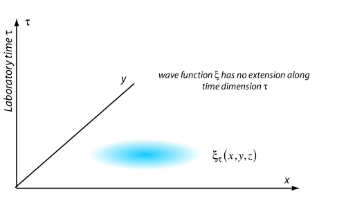
figure-images-int-key-0\hyper@anchorend

We start with the laboratory time or clock time $\tau$, measured by Alice using clocks, laser beams, and graduate students. Laboratory time is defined operationally; in terms of seconds, clock ticks, cycles of a cesium atom. The term is used by Busch ([217]) and others. We will take laboratory time as understood "well enough" for our purposes. (For a deeper examination see, for instance, [573], [939].)

The usual wave function $\xi$  is "flat" in time: it represents a well-defined measure of our uncertainty about the particle’s position in space, but shows no evidence of any uncertainty in time. This seems "unquantum-mechanical". Given that any observer, Bob say, going at high velocity with respect to Alice will mix time and space, what to Alice looks like uncertainty only in space will to Bob look like uncertainty in a blend of time and space.

2.2.2 Quantum Time

Refer to caption
Figure 2.2: Quantum Time
\Hy@raisedlink
\hyper@anchorstart

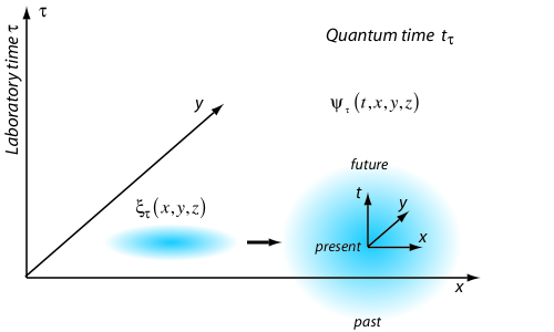
figure-images-int-key-1\hyper@anchorend

If we are to treat time and space symmetrically – our basic assumption – there can be no justification for treating time as flat but space as fuzzy.

We will therefore extrude Alice’s wave function into the time dimension, positing that the wave function, at any given instant, is a function of time as well. Alice will now have to add uncertainty about the particle’s position in time to her existing uncertainty about the particle’s position in space:

\Hy@raisedlink\hyper@anchorstartequationintkeyintkey1\hyper@anchorendξτ(x,y,z)ψτ(t,x,y,z)\Hy@raisedlink\hyper@anchorstart𝑒𝑞𝑢𝑎𝑡𝑖𝑜𝑛𝑖𝑛𝑡𝑘𝑒𝑦𝑖𝑛𝑡𝑘𝑒𝑦1\hyper@anchorendsubscript𝜉𝜏𝑥𝑦𝑧subscript𝜓𝜏𝑡𝑥𝑦𝑧\Hy@raisedlink{\hyper@anchorstart{equation-int-key-int-key-1}\hyper@anchorend}{\xi}_{\tau}\left(x,y,z\right)\rightarrow{\psi}_{\tau}\left(t,x,y,z\right) (2.2)

This extruded wave function represents uncertainty in time and space, just as the wave function normally does in just space. How the extruded wave function depends on quantum time, Latin $t$, is strongly constrained by covariance. Of this much much more below (Formal Development).

To see the effects of the extrusion of the wave function into quantum time $t$, we can treat quantum time like any other unmeasured quantum variable, computing its indirect effects by taking expectations against reduced density matrices and the like 333 Implicit in this use of quantum time is the assumption of the block universe, that all time exists at once ([943], [829], [110], [1075]). While there is no question that this is counter-intuitive, it is difficult to reconcile the more intuitive concept of a fleeting and momentary present with special relativity and its implications for simultaneity. See Petkov for a vigorous defense of this point: [920], [922]. There is evidence for the block universe view within quantum mechanics as well, in the delayed choice quantum eraser ([1030], [688]). The most straightforward way to make sense of this experiment is to see all time as existing at once. Asymmetry between time and space is customary in quantum mechanics, but not mandatory. Aharonov, Bergmann, and Lebowitz have given a time-symmetric approach to measurement [13]. Cramer has given a time-symmetric interpretation of quantum mechanics [278], [280]. There is no quantum arrow of time per Maccone [748]  amended in [749]. .

2.2.3 Relationship of Quantum and Laboratory Time

Hilgevoord cautions us to distinguish between the use of coordinates as parameter and as operator ([583] [584]). For instance, we have x  the coordinate and x  the operator, with different roles in a typical construction:

\Hy@raisedlink\hyper@anchorstartequationintkeyintkey4\hyper@anchorendx(op)dx(coord)ξ(x(coord))x(op)ξ(x(coord))\Hy@raisedlink\hyper@anchorstart𝑒𝑞𝑢𝑎𝑡𝑖𝑜𝑛𝑖𝑛𝑡𝑘𝑒𝑦𝑖𝑛𝑡𝑘𝑒𝑦4\hyper@anchorenddelimited-⟨⟩superscript𝑥𝑜𝑝dsuperscript𝑥𝑐𝑜𝑜𝑟𝑑superscript𝜉superscript𝑥𝑐𝑜𝑜𝑟𝑑superscript𝑥𝑜𝑝𝜉superscript𝑥𝑐𝑜𝑜𝑟𝑑\Hy@raisedlink{\hyper@anchorstart{equation-int-key-int-key-4}\hyper@anchorend}\langle{x}^{\left(op\right)}\rangle\equiv{\displaystyle\int\text{d}{x}^{\left(coord\right)}{\xi}^{\ast}\left({x}^{\left(coord\right)}\right)}{x}^{\left(op\right)}\xi\left({x}^{\left(coord\right)}\right) (2.3)

He argues (correctly in our view) that in standard quantum theory there is no time operator:

If $t$  is not the relativistic partner of q  [the space operator], what is the true partner of the latter? The answer is simply that such a partner does not exist; the position variable of a point particle is a non-covariant concept.

— Jan Hilgevoord and David Atkinson [588]

While time is not an operator in standard quantum theory, in this work – by assumption – it is. We can therefore write:

\Hy@raisedlink\hyper@anchorstartequationintkeyintkey5\hyper@anchorendt(op)dt(coord)dx(coord)ψ(t(coord),x(coord))t(op)ψ(t(coord),x(coord))\Hy@raisedlink\hyper@anchorstart𝑒𝑞𝑢𝑎𝑡𝑖𝑜𝑛𝑖𝑛𝑡𝑘𝑒𝑦𝑖𝑛𝑡𝑘𝑒𝑦5\hyper@anchorenddelimited-⟨⟩superscript𝑡𝑜𝑝dsuperscript𝑡𝑐𝑜𝑜𝑟𝑑dsuperscript𝑥𝑐𝑜𝑜𝑟𝑑superscript𝜓superscript𝑡𝑐𝑜𝑜𝑟𝑑superscript𝑥𝑐𝑜𝑜𝑟𝑑superscript𝑡𝑜𝑝𝜓superscript𝑡𝑐𝑜𝑜𝑟𝑑superscript𝑥𝑐𝑜𝑜𝑟𝑑\Hy@raisedlink{\hyper@anchorstart{equation-int-key-int-key-5}\hyper@anchorend}\langle{t}^{\left(op\right)}\rangle\equiv{\displaystyle\int\text{d}{t}^{\left(coord\right)}\text{d}{x}^{\left(coord\right)}{\psi}^{\ast}\left({t}^{\left(coord\right)},{x}^{\left(coord\right)}\right){t}^{\left(op\right)}\psi\left({t}^{\left(coord\right)},{x}^{\left(coord\right)}\right)} (2.4)

The usual wave function changes shape as laboratory time advances; if it did not it would not be interesting. The quantum time wave function must evolve with laboratory time as well. At each tick of the laboratory clock we expect that $\psi$  will have in general a slightly different shape with respect to quantum time.

It will be (extremely) convenient to define the relative quantum time ${t}_{\tau}$  as the offset in quantum time from the current value of Alice’s laboratory time:

\Hy@raisedlink\hyper@anchorstartequationintkeyconvsymbolsreltime\hyper@anchorendtτtτ\Hy@raisedlink\hyper@anchorstart𝑒𝑞𝑢𝑎𝑡𝑖𝑜𝑛𝑖𝑛𝑡𝑘𝑒𝑦𝑐𝑜𝑛𝑣𝑠𝑦𝑚𝑏𝑜𝑙𝑠𝑟𝑒𝑙𝑡𝑖𝑚𝑒\hyper@anchorendsubscript𝑡𝜏𝑡𝜏\Hy@raisedlink{\hyper@anchorstart{equation-int-key-conv-symbols-reltime}\hyper@anchorend}{t}_{\tau}\equiv t-\tau (2.5)

If the lab clock says 10 seconds past the hour, the relative quantum time might be 10 attoseconds before or after that. In most cases, we expect that the expectation of the quantum time will be approximately equal to the laboratory time and therefore that the expectation of the relative time will be approximately zero:

\Hy@raisedlink\hyper@anchorstartequationintkeyintkey2b\hyper@anchorendtτtτ0\Hy@raisedlink\hyper@anchorstart𝑒𝑞𝑢𝑎𝑡𝑖𝑜𝑛𝑖𝑛𝑡𝑘𝑒𝑦𝑖𝑛𝑡𝑘𝑒𝑦2𝑏\hyper@anchorendsimilar-todelimited-⟨⟩𝑡𝜏similar-todelimited-⟨⟩subscript𝑡𝜏0\Hy@raisedlink{\hyper@anchorstart{equation-int-key-int-key-2b}\hyper@anchorend}\begin{array}[]{l}\langle t\rangle\sim\tau\\ \langle{t}_{\tau}\rangle\sim 0\end{array} (2.6)

The situation is analogous to the use of "center of mass" coordinates. We use center of mass coordinates to subtract off the average value of the space coordinates, letting us focus on the interesting part. And we can use "center of time" coordinates the same way, to focus on what is essential.

As an example, suppose Alice is travelling by train from Berne to Zurich. She decides to while away the time by doing quantum mechanics experiments (we are not explaining, merely reporting). If she is doing, say, a standard double slit experiment, then she will compute x, y, and z  relative to her current location on the train. An outside observer, say Bob, might compute his x  as the sum of the train’s x  and Alice’s x. Alice’s x  may be thought of as a relative space coordinate. The same with time. Alice may find it convenient to compute her experimental times in terms of attoseconds; Bob may compute the times as the clock time in the train plus the attoseconds. Alice is then using relative time; Bob is using block time.

With quantum time we are not  inventing a new time dimension or assigning new properties to the existing time dimension. We are merely treating, for purposes of quantum mechanics, time the same as the three space dimensions.

2.2.4 Evolution of the Wave Function

Refer to caption
Figure 2.3: Evolution of Wave Function
\Hy@raisedlink
\hyper@anchorstart

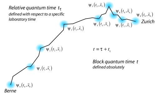
figure-images-int-key-2\hyper@anchorend

How are we to compute the wave function at the next tick of the laboratory clock when we know it at the current clock tick? We need dynamics.

We will use Feynman path integrals as our defining methodology; we will derive the Schrödinger equation, operator mechanics, and canonical path integrals from them 444Particularly readable introductions to Feynman path integrals are found in [402]  and [1017]..

A path in the usual three dimensional Feynman path integrals is defined as a series of coordinate locations; to specify the path we specify a specific location in three space at each tick of the laboratory clock. To do the path integral we sum over all such paths using an appropriate weighting factor.

In temporal quantization we specify the paths as a specific location in four space – time plus the three space dimensions – at each tick of the laboratory clock. To do the path integral we sum over all such paths using an appropriate weighting factor. Curiously enough, we can use the same weighting factor  in temporal quantization as in standard quantum theory.

The paths in temporal quantization can be a bit ahead or behind the laboratory time; they can – and typically will – have a non-zero relative time. We will have to first show that these effects normally average out (or else someone would have seen them); we will then show that with a bit of ingenuity they should be detectable.

In Feynman path integrals we do not normally use a continuous laboratory time; we break it up into slices and then let the number of slices go to infinity. We can see each slice as corresponding to a frame in a movie. The laboratory time functions as an index, like the frame count in a movie. It is not part of the dynamics. Laboratory time is time as parameter.

If Alice is walking her dog, her path corresponds to laboratory time, a smooth steadily increasing progression. Her dog’s path corresponds to quantum time, frisking ahead or behind at any moment, but still centered on the laboratory time 555Of course, Alice is herself a quantum mechanical system, made of atoms and their bonds. Alice’s own wave function is a product of the many many wave functions of her particles, amino acids, sugars, water molecules, and so on. Her average quantum time will be almost exactly her laboratory time..

2.3 Literature

\Hy@raisedlink\hyper@anchorstart

int-lit\hyper@anchorend

With 2500 years to work up a running start, the literature on time is enormous. Popular discussions include: [230], [231], [480], [312], [603], [367], [1123], [314], [563], [566], [564], [945], [829], [1133], [110], [1075], [444], [545], [657], [234]; more technical include: [970], [897], [277], [898], [561], [541], [750], [845], [852], [999], [1019], [103], [700], [1237], [824], [1241], [1245], [511], [676], [524], [112].

The approach we are taking here is most similar to some work by Feynman ([399] [400]). Note particularly his variation on the Klein-Gordon equation:

\Hy@raisedlink\hyper@anchorstartequationintlitintlit0\hyper@anchorendiψu(x)u=12(ixμeAμ)(ixμeAμ)ψu(x)\Hy@raisedlink\hyper@anchorstart𝑒𝑞𝑢𝑎𝑡𝑖𝑜𝑛𝑖𝑛𝑡𝑙𝑖𝑡𝑖𝑛𝑡𝑙𝑖𝑡0\hyper@anchorend𝑖subscript𝜓𝑢𝑥𝑢12𝑖superscript𝑥𝜇𝑒subscript𝐴𝜇𝑖subscript𝑥𝜇𝑒superscript𝐴𝜇subscript𝜓𝑢𝑥\Hy@raisedlink{\hyper@anchorstart{equation-int-lit-int-lit-0}\hyper@anchorend}i\frac{\partial{\psi}_{u}\left(x\right)}{\partial u}=-\frac{1}{2}\left(i\frac{\partial}{\partial{x}^{\mu}}-e{A}_{\mu}\right)\left(i\frac{\partial}{\partial{x}_{\mu}}-e{A}^{\mu}\right){\psi}_{u}\left(x\right) (2.7)

Where u  is a formal time parameter "somewhat analogous to proper time".

Using proper time makes it difficult to handle multiple particles – whose proper time should we use? – hence our preference for using laboratory time as a starting point.

We see some resemblances of our propagators and Schrödinger equation to the Stuckelberg propagator and Schrödinger equation used by Land and by Horwitz ([716] [609]). They add a fifth parameter, treated dynamically, so that it takes part in gauge transformations and the like. Another fifth parameter formalism is found in [1036]. There is an ongoing series of conferences on such: [464].

The principal difference between fifth parameter formalisms in general and quantum time here is that here we have only four parameters: laboratory time and quantum time have to share: they are really only different views of a single time dimension. Neither is formal; both are real.

Among the many other variations on the theme of time are: stochastic time [181], random time [262], complex time [85], discrete times [141] [636] [954] [297], labyrinthean time [545], multiple time dimensions [250], [1066], [1192], time generated from within the observer – internal time [1098], and most recently crystallizing time [382].

There is an excellent summary of possible times in a Scientific American article by Max Tegmark [1113]. He describes massively parallel time, forking time, distant times, and more.

There is no end to alternate times: in his novel Einstein’s Dreams [733]  A. Lightman imagines A. Einstein imagining thirty or more different kinds of times, before settling on relativity.

Temporal quantization – as we will refer to the process of quantizing along the time dimensions – plays nicely with many of these variations on the theme of time. For instance we assume time is smooth. But suppose time is quantized at the scale of the Planck time:

\Hy@raisedlink\hyper@anchorstartequationintlitintlit1\hyper@anchorendt(Planck)Gc55.39x1044s\Hy@raisedlink\hyper@anchorstart𝑒𝑞𝑢𝑎𝑡𝑖𝑜𝑛𝑖𝑛𝑡𝑙𝑖𝑡𝑖𝑛𝑡𝑙𝑖𝑡1\hyper@anchorendsuperscript𝑡𝑃𝑙𝑎𝑛𝑐𝑘Planck-constant-over-2-pi𝐺superscript𝑐55.39𝑥superscript1044𝑠\Hy@raisedlink{\hyper@anchorstart{equation-int-lit-int-lit-1}\hyper@anchorend}{t}^{\left(Planck\right)}\equiv\sqrt{\frac{\hslash G}{{c}^{5}}}\approx 5.39x{10}^{-44}s (2.8)

We would only insist that space be quantized in the same way, at the scale of the Planck length:

\Hy@raisedlink\hyper@anchorstartequationintlitintlit2\hyper@anchorendl(Planck)ct(Planck)=Gc31.62x1035m\Hy@raisedlink\hyper@anchorstart𝑒𝑞𝑢𝑎𝑡𝑖𝑜𝑛𝑖𝑛𝑡𝑙𝑖𝑡𝑖𝑛𝑡𝑙𝑖𝑡2\hyper@anchorendsuperscript𝑙𝑃𝑙𝑎𝑛𝑐𝑘𝑐superscript𝑡𝑃𝑙𝑎𝑛𝑐𝑘Planck-constant-over-2-pi𝐺superscript𝑐31.62𝑥superscript1035𝑚\Hy@raisedlink{\hyper@anchorstart{equation-int-lit-int-lit-2}\hyper@anchorend}{l}^{\left(Planck\right)}\equiv c{t}^{\left(Planck\right)}=\sqrt{\frac{\hslash G}{{c}^{3}}}\approx 1.62x{10}^{-35}m (2.9)

2.4 Plan of Attack

\Hy@raisedlink\hyper@anchorstart

int-plan\hyper@anchorend

Refer to caption
Figure 2.4: Objective: a Manifestly Covariant Quantum Mechanics
\Hy@raisedlink
\hyper@anchorstart

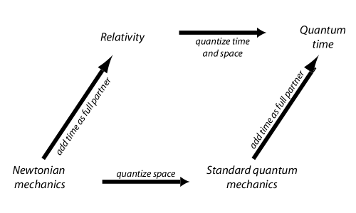
figure-images-int-plan-0\hyper@anchorend

2.4.1 Organization

In the interests of biting off a "testable chunk", we will only look at the single particle case here. We will do so in a way that does not exclude extending the ideas to multiple particles.

We primarily interested in "proof-of-concept" here, so we will only look at the lowest nontrivial corrections resulting from quantum time.

We have organized the rest of this paper in roughly the order of the five requirements, that temporal quantization be:

  1. 1.

    Well-defined,

  2. 2.

    Manifestly covariant,

  3. 3.

    Consistent with known experimental results,

  4. 4.

    Testable,

  5. 5.

    And reasonably simple.

By chapters:

  1. 1.

    In Formal Development, we work out the formalism, using path integrals and the requirement of manifest covariance (Feynman Path Integrals).

    We use the path integral result to derive the Schrödinger equation in four dimensions (Derivation of the Schrödinger Equation). We use the Schrödinger equation to prove unitarity (Unitarity) and to analyze the effect of gauge transformations (Gauge Transformations for the Schrödinger Equation).

    We derive an operator formalism from the Schrödinger equation (Operators in Time), then derive the canonical path integral from the operator formalism (Derivation of the Canonical Path Integral).

    From the canonical path integral we derive the Feynman path integral (Closing the Circle), closing the circle.

    All four formalisms make use of the laboratory time; in a final section, Covariant Definition of Laboratory Time, we show we can define the laboratory time in a way which is covariant, thereby establishing full covariance of the formalisms.

    This establishes that temporal quantization is well-defined (in a formal sense) and covariant (by construction).

  2. 2.

    In Comparison of Temporal Quantization To Standard Quantum Theory, we look at various limits in which we recover standard quantum theory from temporal quantization:

    1. (a)

      The Non-relativistic Limit,

    2. (b)

      The Semi-classical Limit,

    3. (c)

      And the Long Time Limit.

  3. 3.

    In Experimental Tests, we look at a starter set of experimental tests.

    In general, to see an effect of temporal quantization both  beam and apparatus should vary in time. With this condition met, temporal quantization will tend to produce increased dispersion in time and – occasionally – slightly different interference patterns.

    We look at the cases of:

    1. (a)

      Slits in Time,

    2. (b)

      Time-varying Magnetic and Electric Fields,

    3. (c)

      And the Aharonov-Bohm Experiment.

    These experiments establish that:

    • Temporal quantization is well-defined in an operational sense; its formalism can be mapped into well-defined counts of clicks in a detector.

    • Temporal quantization is testable.

  4. 4.

    Finally, in the Discussion  we summarize the analysis, argue that temporal quantization has met the requirements, and look at further areas for investigation.

Post-finally, we summarize some useful facts about free wave functions in an appendix Free Particles.

2.4.2 Notations and Conventions

  1. 1.

    We use Latin $t$  for quantum time; Greek $\tau$  for laboratory time.

  2. 2.

    We use an over-dot for the derivative with respect to laboratory time, e.g:

    \Hy@raisedlink\hyper@anchorstartequationintplanconvsymbolsoverdot\hyper@anchorendχ˙τddτχτ\Hy@raisedlink\hyper@anchorstart𝑒𝑞𝑢𝑎𝑡𝑖𝑜𝑛𝑖𝑛𝑡𝑝𝑙𝑎𝑛𝑐𝑜𝑛𝑣𝑠𝑦𝑚𝑏𝑜𝑙𝑠𝑜𝑣𝑒𝑟𝑑𝑜𝑡\hyper@anchorendsubscript˙𝜒𝜏𝑑𝑑𝜏subscript𝜒𝜏\Hy@raisedlink{\hyper@anchorstart{equation-int-plan-conv-symbols-overdot}\hyper@anchorend}{\dot{\chi}}_{\tau}\equiv\frac{d}{d\tau}{\chi}_{\tau} (2.10)
  3. 3.

    We use an over-bar to indicate averaging. We also use an over-bar to indicate the standard quantum theory/space part of an object.

    We use a ’frown’ character ($\frown$) to indicate the quantum time part.

    We use the absence of a mark to mark a fully four dimensional   object.

    For example, we will see that the free kernel can be written as a product of time and space parts:

    \Hy@raisedlink\hyper@anchorstartequationintplanconvsymbols3\hyper@anchorendKτ(free)(t′′,x′′;t,x)=Kτ(free)(t′′;t)K¯τ(free)(x′′;x)\Hy@raisedlink{\hyper@anchorstart{equation-int-plan-conv-symbols-3}\hyper@anchorend}{K}_{\tau}^{\left(free\right)}\left({t}^{{{}^{\prime\prime}}},{\overrightarrow{x}}^{{{}^{\prime\prime}}};{t}^{\prime},{\overrightarrow{x}}^{\prime}\right)={\stackrel{{\scriptstyle\frown}}{{K}}}_{\tau}^{\left(free\right)}\left({t}^{{{}^{\prime\prime}}};{t}^{\prime}\right){\overline{K}}_{\tau}^{\left(free\right)}\left({\overrightarrow{x}}^{{{}^{\prime\prime}}};{\overrightarrow{x}}^{\prime}\right) (2.11)
  4. 4.

    When we can, we will use $\chi$  for the time part of wave functions (from the initial letter of $\chi\rho\acute{o}\nu o\varsigma$, the Greek word for time), and $\xi$  (Greek x) for the space part, e.g.:

    \Hy@raisedlink\hyper@anchorstartequationintplanconvsymbols2\hyper@anchorendψτ(t,x)=χτ(t)ξτ(x)\Hy@raisedlink\hyper@anchorstart𝑒𝑞𝑢𝑎𝑡𝑖𝑜𝑛𝑖𝑛𝑡𝑝𝑙𝑎𝑛𝑐𝑜𝑛𝑣𝑠𝑦𝑚𝑏𝑜𝑙𝑠2\hyper@anchorendsubscript𝜓𝜏𝑡𝑥subscript𝜒𝜏𝑡subscript𝜉𝜏𝑥\Hy@raisedlink{\hyper@anchorstart{equation-int-plan-conv-symbols-2}\hyper@anchorend}{\psi}_{\tau}\left(t,\overrightarrow{x}\right)={\chi}_{\tau}\left(t\right){\xi}_{\tau}\left(\overrightarrow{x}\right) (2.12)

We will be using natural units, c  and $\hslash$  set to one, except as explicitly noted.

In an effort to reduce notational clutter we will:

  1. 1.

    Use two indexes together to mean the difference of the first indexed variable and the second:

    \Hy@raisedlink\hyper@anchorstartequationintplanconvsymbolsshort1\hyper@anchorendτBAτBτA\Hy@raisedlink\hyper@anchorstart𝑒𝑞𝑢𝑎𝑡𝑖𝑜𝑛𝑖𝑛𝑡𝑝𝑙𝑎𝑛𝑐𝑜𝑛𝑣𝑠𝑦𝑚𝑏𝑜𝑙𝑠𝑠𝑜𝑟𝑡1\hyper@anchorendsubscript𝜏𝐵𝐴subscript𝜏𝐵subscript𝜏𝐴\Hy@raisedlink{\hyper@anchorstart{equation-int-plan-conv-symbols-short1}\hyper@anchorend}{\tau}_{BA}\equiv{\tau}_{B}-{\tau}_{A} (2.13)
  2. 2.

    Replace an indexed laboratory time, e.g. ${\tau}_{\text{A}}$, with its index, e.g. A, when we can do so without loss of clarity:

    \Hy@raisedlink\hyper@anchorstartequationintplanconvsymbolsshort2\hyper@anchorendψAψτA\Hy@raisedlink\hyper@anchorstart𝑒𝑞𝑢𝑎𝑡𝑖𝑜𝑛𝑖𝑛𝑡𝑝𝑙𝑎𝑛𝑐𝑜𝑛𝑣𝑠𝑦𝑚𝑏𝑜𝑙𝑠𝑠𝑜𝑟𝑡2\hyper@anchorendsubscript𝜓𝐴subscript𝜓subscript𝜏𝐴\Hy@raisedlink{\hyper@anchorstart{equation-int-plan-conv-symbols-short2}\hyper@anchorend}{\psi}_{A}\equiv{\psi}_{{\tau}_{A}} (2.14)

For the square root of complex numbers we use a branch cut from zero to negative infinity.

We use the Einstein summation convention with Greek indices being summed from 0 to 3, Latin from 1 to 3.

Chapter 3 Formal Development

\Hy@raisedlink\hyper@anchorstart

tq\hyper@anchorend

3.1 Overview

\Hy@raisedlink\hyper@anchorstart

tq-intro\hyper@anchorend

The rules of quantum mechanics and special relativity are so strict and powerful that it’s very hard to build theories that obey both.

— Frank Wilczek [1215]

Now we could travel anywhere we wanted to go. All a man had to do was to think of what he says and to look where he was going.

— The Legend of the Flying Canoe [355]

Refer to caption
Figure 3.1: Four Formalisms
\Hy@raisedlink
\hyper@anchorstart

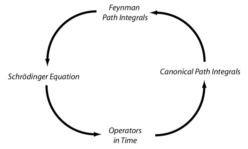
figure-images-tq-disc-0\hyper@anchorend

In this chapter we develop the formal rules for temporal quantization. Like a snake headed out for its morning rat, we will need to take some twists and turns to get to our objective. We use Feynman path integrals  as the defining formalism. Comprehensive treatments of path integrals are provided in: [403], [1017], [1101], [672], [694], [1249].

We will derive three other formalisms, each in turn, from the Feynman path integrals:

  1. 1.

    Schrödinger Equation,

  2. 2.

    Operators in Time,

  3. 3.

    And Canonical Path Integrals.

We will close the circle by deriving the Feynman path integral from the canonical path integral.

All four approaches make use of the laboratory time. To get a completely covariant treatment we need to define the laboratory time in a covariant way as well. The proper time of the particle will not do; what if we have many particles? What of virtual particles, those evanescent dolphins of the Bose and Fermi seas? What of the massless and therefore timeless photons?

Instead in the last section of this chapter, Covariant Definition of Laboratory Time, we break the initial wave function down using Morlet wavelet decomposition ([817], [261], [796], [651], [1152], [5], [192], [75], [96]), then evolve each part along its own personal classical path to its destined detector. These classical paths each have a well-defined proper time which will serve as the laboratory time for the part. At the detector, we assemble the parts back into one self-consistent whole.

With this done, we will have satisfied the first two requirements (The Problem of Time), that temporal quantization be:

  1. 1.

    Well-defined

  2. 2.

    And manifestly covariant.

3.2 Feynman Path Integrals

\Hy@raisedlink\hyper@anchorstart

tq-fpi\hyper@anchorend

The path integral method is perhaps the most elegant and powerful of all quantization programs.

— Michio Kaku [654]

Furthermore, we wish to emphasize that in future in all cities, markets and in the country, the only ingredients used for the brewing of beer must be Barley, Hops and Water. Whosoever knowingly disregards or transgresses upon this ordinance, shall be punished by the Court authorities’ confiscating such barrels of beer, without fail.

— Duke of Bavaria [366]

Refer to caption
Figure 3.2: Path Integrals
\Hy@raisedlink
\hyper@anchorstart

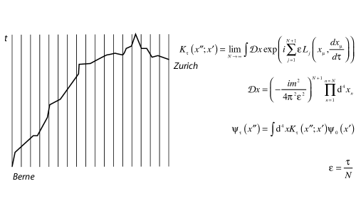
figure-images-tq-fpi-0\hyper@anchorend

With path integrals as with beer, all we need to get good results are a few simple ingredients, a recipe for combining them, and a bit of time. For path integrals the ingredients are the initial wave functions, the paths, and a Lagrangian; the recipe is the procedure for summing over the paths 111Usually we would start an analysis with the Schrödinger equation and then derive the kernel as its inverse. Here it is more natural to start with the path integral expression for the kernel then derive the Schrödinger equation from that..

Our guiding principle is manifest covariance. We look at:

  1. 1.

    The Wave Functions,

  2. 2.

    The Paths,

  3. 3.

    The Lagrangian,

  4. 4.

    The Sum over Paths,

  5. 5.

    How to ensure Convergence  of the sum over paths,

  6. 6.

    How to ensure correct Normalization,

  7. 7.

    And the Formal Expression for the Path Integral.

3.2.1 Wave Functions

\Hy@raisedlink\hyper@anchorstart

tq-fpi-waves\hyper@anchorend

Requirements

To define our wave functions we need a basis which is:

  1. 1.

    Non-singular,

  2. 2.

    General,

  3. 3.

    And reasonably simple.

Plane Waves

Using a Fourier decomposition in time is general but problematic. The use of singular functions or non-normalizable functions, e.g. plane waves or $\delta$  functions, may introduce artifacts 222A further disadvantage of using plane waves as the basis functions is that demonstrating the convergence of our path integrals then becomes tricky, as will be discussed below Convergence.. It is safer to use more physical wave functions, i.e. wave packets.

There is a good example of the benefits of using more realistic wave functions in Gondran and Gondran, [493]. When they analyze the Stern-Gerlach experiment using a Gaussian initial wave function (as opposed to a plane wave) they see the usual split of the beam – without any need to invoke the notorious and troubling "collapse of the wave function".

An implication of Gondran and Gondran’s work is that some of the difficulties in the analysis of the measurement problem may be the result not of problems with quantum mechanics per se but rather of using unphysical approximations.

This is an implication of the program of decoherence as well.

The assumption that we can isolate a quantum system from its environment is unphysical. The program of decoherence (see [1236], [472], [1007]  and references therein) has been able to explain much of the "problem of measurement" by relaxing this assumption, by explicitly including interactions with the environment in the analysis.

Avoiding unphysical assumptions is as important in the analysis of time as of measurement. Time is already a subtle and difficult subject; we do not want to introduce any unnecessary complexities, especially not at the start.

Wave Packets

Wave packets are more physical but are not general.

Consider an incoming beam, say of electrons. A typical wave packet might look like:

\Hy@raisedlink\hyper@anchorstartequationtqfpiwavestqfpiwaves0\hyper@anchorendψτ(x)=1πσ124exp(iωτ+ikx(xx0)22σ12)\Hy@raisedlink\hyper@anchorstart𝑒𝑞𝑢𝑎𝑡𝑖𝑜𝑛𝑡𝑞𝑓𝑝𝑖𝑤𝑎𝑣𝑒𝑠𝑡𝑞𝑓𝑝𝑖𝑤𝑎𝑣𝑒𝑠0\hyper@anchorendsubscript𝜓𝜏𝑥41𝜋superscriptsubscript𝜎12exp𝑖𝜔𝜏𝑖𝑘𝑥superscript𝑥subscript𝑥022superscriptsubscript𝜎12\Hy@raisedlink{\hyper@anchorstart{equation-tq-fpi-waves-tq-fpi-waves-0}\hyper@anchorend}{\psi}_{\tau}\left(x\right)=\sqrt[4]{\frac{1}{\pi{\sigma}_{1}^{2}}}\mathrm{exp}\left(-i\omega\tau+ikx-\frac{{\left(x-{x}_{0}\right)}^{2}}{2{\sigma}_{1}^{2}}\right) (3.1)

We could generalize the time part by adding a bit of dispersion along our hypothesized quantum time axis:

\Hy@raisedlink\hyper@anchorstartequationtqfpiwavestqfpiwaves1\hyper@anchorendψτ(t,x)1π2σ02σ124exp(iωt(tτ)22σ02+ikx(xx0)22σ12)similar-to\Hy@raisedlink\hyper@anchorstart𝑒𝑞𝑢𝑎𝑡𝑖𝑜𝑛𝑡𝑞𝑓𝑝𝑖𝑤𝑎𝑣𝑒𝑠𝑡𝑞𝑓𝑝𝑖𝑤𝑎𝑣𝑒𝑠1\hyper@anchorendsubscript𝜓𝜏𝑡𝑥41superscript𝜋2superscriptsubscript𝜎02superscriptsubscript𝜎12exp𝑖𝜔𝑡superscript𝑡𝜏22superscriptsubscript𝜎02𝑖𝑘𝑥superscript𝑥subscript𝑥022superscriptsubscript𝜎12\Hy@raisedlink{\hyper@anchorstart{equation-tq-fpi-waves-tq-fpi-waves-1}\hyper@anchorend}{\psi}_{\tau}\left(t,x\right)\sim\sqrt[4]{\frac{1}{{\pi}^{2}{\sigma}_{0}^{2}{\sigma}_{1}^{2}}}\mathrm{exp}\left(-i\omega t-\frac{{\left(t-\tau\right)}^{2}}{2{\sigma}_{0}^{2}}+ikx-\frac{{\left(x-{x}_{0}\right)}^{2}}{2{\sigma}_{1}^{2}}\right) (3.2)

If the $\sigma$’s are large, we may think of this as a gently rounded plane wave.

This is physically reasonable, but not general. Not every wave function is a Gaussian.

Morlet Wavelet Decomposition
Refer to caption
Figure 3.3: Typical Morlet Wavelet
\Hy@raisedlink
\hyper@anchorstart

figure-images-mor-intro-0\hyper@anchorend

To make this general, we recall that any square-integrable wave function may be written as a sum over Morlet wavelets 333Morlet’s initial reference is: [817]. Good discussions of Morlet wavelets and wavelets in general are found in [261], [796], [651], [1152], [5], [192], [75].. We can then break an arbitrary square-integrable wave function up into its component wavelets, propagate each wavelet individually, then sum over the wavelets at the end.

A Morlet wavelet in one dimension has the form:

\Hy@raisedlink\hyper@anchorstartequationtqfpiwavesconvtransmw\hyper@anchorendϕsd(t)=1|s|(ei(tds)1e)e12(tds)2\Hy@raisedlink\hyper@anchorstart𝑒𝑞𝑢𝑎𝑡𝑖𝑜𝑛𝑡𝑞𝑓𝑝𝑖𝑤𝑎𝑣𝑒𝑠𝑐𝑜𝑛𝑣𝑡𝑟𝑎𝑛𝑠𝑚𝑤\hyper@anchorendsubscriptitalic-ϕ𝑠𝑑𝑡1𝑠superscript𝑒𝑖𝑡𝑑𝑠1𝑒superscript𝑒12superscript𝑡𝑑𝑠2\Hy@raisedlink{\hyper@anchorstart{equation-tq-fpi-waves-conv-trans-mw}\hyper@anchorend}{\phi}_{sd}\left(t\right)=\frac{1}{\sqrt{\left|s\right|}}\left({e}^{-i\left(\frac{t-d}{s}\right)}-\frac{1}{\sqrt{e}}\right){e}^{-\frac{1}{2}{\left(\frac{t-d}{s}\right)}^{2}} (3.3)

Here s  is the scale and d  is the displacement. The wavelet with scale one and displacement zero is the mother wavelet:

\Hy@raisedlink\hyper@anchorstartequationtqfpiwavesconvtransmother\hyper@anchorendϕ(mom)(t)=(eit1e)e12t2\Hy@raisedlink\hyper@anchorstart𝑒𝑞𝑢𝑎𝑡𝑖𝑜𝑛𝑡𝑞𝑓𝑝𝑖𝑤𝑎𝑣𝑒𝑠𝑐𝑜𝑛𝑣𝑡𝑟𝑎𝑛𝑠𝑚𝑜𝑡𝑒𝑟\hyper@anchorendsuperscriptitalic-ϕ𝑚𝑜𝑚𝑡superscript𝑒𝑖𝑡1𝑒superscript𝑒12superscript𝑡2\Hy@raisedlink{\hyper@anchorstart{equation-tq-fpi-waves-conv-trans-mother}\hyper@anchorend}{\phi}^{\left(mom\right)}\left(t\right)=\left({e}^{-it}-\frac{1}{\sqrt{e}}\right){e}^{-\frac{1}{2}{t}^{2}} (3.4)

All wavelets are derived from her by changing the values of s  and d:

\Hy@raisedlink\hyper@anchorstartequationtqfpiwavesconvtransscale\hyper@anchorendϕsd(t)=1|s|ϕ(mom)(tds)\Hy@raisedlink\hyper@anchorstart𝑒𝑞𝑢𝑎𝑡𝑖𝑜𝑛𝑡𝑞𝑓𝑝𝑖𝑤𝑎𝑣𝑒𝑠𝑐𝑜𝑛𝑣𝑡𝑟𝑎𝑛𝑠𝑠𝑐𝑎𝑙𝑒\hyper@anchorendsubscriptitalic-ϕ𝑠𝑑𝑡1𝑠superscriptitalic-ϕ𝑚𝑜𝑚𝑡𝑑𝑠\Hy@raisedlink{\hyper@anchorstart{equation-tq-fpi-waves-conv-trans-scale}\hyper@anchorend}{\phi}_{sd}\left(t\right)=\frac{1}{\sqrt{\left|s\right|}}{\phi}^{\left(mom\right)}\left(\frac{t-d}{s}\right) (3.5)

The Morlet wavelet components of a square-integrable wave function f  are:

\Hy@raisedlink\hyper@anchorstartequationtqfpiwavesconvtransmwanalysis\hyper@anchorendf~sd=dtϕsd(t)f(t)\Hy@raisedlink\hyper@anchorstart𝑒𝑞𝑢𝑎𝑡𝑖𝑜𝑛𝑡𝑞𝑓𝑝𝑖𝑤𝑎𝑣𝑒𝑠𝑐𝑜𝑛𝑣𝑡𝑟𝑎𝑛𝑠𝑚subscript𝑤𝑎𝑛𝑎𝑙𝑦𝑠𝑖𝑠\hyper@anchorendsubscript~𝑓𝑠𝑑infinityd𝑡superscriptsubscriptitalic-ϕ𝑠𝑑𝑡𝑓𝑡\Hy@raisedlink{\hyper@anchorstart{equation-tq-fpi-waves-conv-trans-mw_{a}nalysis}\hyper@anchorend}{\tilde{f}}_{sd}={\displaystyle\underset{-\infty}{\overset{\infty}{\int}}\text{d}t{\phi}_{sd}^{\ast}\left(t\right)f\left(t\right)} (3.6)

To recover the original wave function f  from the Morlet wavelet components ${\tilde{f}}_{sd}$:

\Hy@raisedlink\hyper@anchorstartequationtqfpiwavesconvtransmwsynthesis\hyper@anchorendf(t)=1Cdsdds2ϕsd(t)f~sd\Hy@raisedlink\hyper@anchorstart𝑒𝑞𝑢𝑎𝑡𝑖𝑜𝑛𝑡𝑞𝑓𝑝𝑖𝑤𝑎𝑣𝑒𝑠𝑐𝑜𝑛𝑣𝑡𝑟𝑎𝑛𝑠𝑚subscript𝑤𝑠𝑦𝑛𝑡𝑒𝑠𝑖𝑠\hyper@anchorend𝑓𝑡1𝐶infinityd𝑠d𝑑superscript𝑠2subscriptitalic-ϕ𝑠𝑑𝑡subscript~𝑓𝑠𝑑\Hy@raisedlink{\hyper@anchorstart{equation-tq-fpi-waves-conv-trans-mw_{s}ynthesis}\hyper@anchorend}f\left(t\right)=\frac{1}{C}{\displaystyle\underset{-\infty}{\overset{\infty}{\int}}\frac{\text{d}s\text{d}d}{{s}^{2}}{\phi}_{sd}\left(t\right){\tilde{f}}_{sd}} (3.7)

C, the "admissibility constant", is computed in [96].

As each Morlet wavelet is a sum over two Gaussians, any normalizable function may be decomposed into a sum over Gaussians.

Therefore, to compute the path integral results for an arbitrary normalizable wave function, we use Morlet wavelet analysis to decompose it into Gaussian test functions, compute the result for each Gaussian test function, then sum to get the full result.

Gaussian Test Functions

A Gaussian test function (a squeezed state) in x  is defined by its values for the average x, average p, and dispersion in x. For a four dimensional function, x  and p  are vectors and the dispersion is a four-by-four matrix. Therefore there are potentially four plus four plus sixteen or twenty-four of these values. For test functions we will always use a diagonal dispersion matrix, letting us write our test functions as direct products of functions in $t$, x, y, and z:

\Hy@raisedlink\hyper@anchorstartequationtqfpiwavesfreefourtphi0\hyper@anchorendψ0(x)=1π4det(Σ0)4exp(ipμ(0)xμ12Σ0μν(xμx¯0μ)(xnx¯0ν))\Hy@raisedlink\hyper@anchorstart𝑒𝑞𝑢𝑎𝑡𝑖𝑜𝑛𝑡𝑞𝑓𝑝𝑖𝑤𝑎𝑣𝑒𝑠𝑓𝑟𝑒𝑒𝑓𝑜𝑢𝑟𝑡𝑝𝑖0\hyper@anchorendsubscript𝜓0𝑥41superscript𝜋4detsubscriptΣ0exp𝑖superscriptsubscript𝑝𝜇0superscript𝑥𝜇12superscriptsubscriptΣ0𝜇𝜈superscript𝑥𝜇superscriptsubscript¯𝑥0𝜇superscript𝑥𝑛superscriptsubscript¯𝑥0𝜈\Hy@raisedlink{\hyper@anchorstart{equation-tq-fpi-waves-free-fourt-phi0}\hyper@anchorend}{\psi}_{0}\left(x\right)=\sqrt[4]{\frac{1}{{\pi}^{4}\mathrm{det}\left({\Sigma}_{0}\right)}}\mathrm{exp}\left(-i{p}_{\mu}^{\left(0\right)}{x}^{\mu}-\frac{1}{2{\Sigma}_{0}^{\mu\nu}}\left({x}^{\mu}-{\overline{x}}_{0}^{\mu}\right)\left({x}^{n}-{\overline{x}}_{0}^{\nu}\right)\right) (3.8)

With the definition of the dispersion matrix:

\Hy@raisedlink\hyper@anchorstartequationtqfpiwavesfreefourtsigma0\hyper@anchorendΣ0μν=(σ020000σ120000σ220000σ32)\Hy@raisedlink\hyper@anchorstart𝑒𝑞𝑢𝑎𝑡𝑖𝑜𝑛𝑡𝑞𝑓𝑝𝑖𝑤𝑎𝑣𝑒𝑠𝑓𝑟𝑒𝑒𝑓𝑜𝑢𝑟𝑡𝑠𝑖𝑔𝑚𝑎0\hyper@anchorendsuperscriptsubscriptΣ0𝜇𝜈superscriptsubscript𝜎020000superscriptsubscript𝜎120000superscriptsubscript𝜎220000superscriptsubscript𝜎32\Hy@raisedlink{\hyper@anchorstart{equation-tq-fpi-waves-free-fourt-sigma0}\hyper@anchorend}{\Sigma}_{0}^{\mu\nu}=\left(\begin{array}[]{cccc}{\sigma}_{0}^{2}&0&0&0\\ 0&{\sigma}_{1}^{2}&0&0\\ 0&0&{\sigma}_{2}^{2}&0\\ 0&0&0&{\sigma}_{3}^{2}\end{array}\right) (3.9)

And only twelve free parameters, three per dimension.

We can break this out into time and space parts. We use $\chi$  for the time part, $\xi$  for the space part:

\Hy@raisedlink\hyper@anchorstartequationtqfpiwavesfreefourtbreakout\hyper@anchorendψ0(t,x)=χ0(t)ξ0(x)\Hy@raisedlink\hyper@anchorstart𝑒𝑞𝑢𝑎𝑡𝑖𝑜𝑛𝑡𝑞𝑓𝑝𝑖𝑤𝑎𝑣𝑒𝑠𝑓𝑟𝑒𝑒𝑓𝑜𝑢𝑟𝑡𝑏𝑟𝑒𝑎𝑘𝑜𝑢𝑡\hyper@anchorendsubscript𝜓0𝑡𝑥subscript𝜒0𝑡subscript𝜉0𝑥\Hy@raisedlink{\hyper@anchorstart{equation-tq-fpi-waves-free-fourt-breakout}\hyper@anchorend}{\psi}_{0}\left(t,x\right)={\chi}_{0}\left(t\right){\xi}_{0}\left(\overrightarrow{x}\right) (3.10)

Time part:

\Hy@raisedlink\hyper@anchorstartequationtqfpiwavesfreeonetchi0\hyper@anchorendχ0(t)=1πσ024exp(iE0t12σ02(tt¯0)2)\Hy@raisedlink\hyper@anchorstart𝑒𝑞𝑢𝑎𝑡𝑖𝑜𝑛𝑡𝑞𝑓𝑝𝑖𝑤𝑎𝑣𝑒𝑠𝑓𝑟𝑒𝑒𝑜𝑛𝑒𝑡𝑐𝑖0\hyper@anchorendsubscript𝜒0𝑡41𝜋superscriptsubscript𝜎02exp𝑖subscript𝐸0𝑡12superscriptsubscript𝜎02superscript𝑡subscript¯𝑡02\Hy@raisedlink{\hyper@anchorstart{equation-tq-fpi-waves-free-onet-chi0}\hyper@anchorend}{\chi}_{0}\left(t\right)=\sqrt[4]{\frac{1}{\pi{\sigma}_{0}^{2}}}\mathrm{exp}\left(-i{E}_{0}t-\frac{1}{2{\sigma}_{0}^{2}}{\left(t-{\overline{t}}_{0}\right)}^{2}\right) (3.11)

Space part:

\Hy@raisedlink\hyper@anchorstartequationtqfpiwavesfreefourtxi0\hyper@anchorendξ0(x)=1π3det(Σij(0))4exp(ip0x(xx0)i12Σij(0)(xx0)j)\Hy@raisedlink\hyper@anchorstart𝑒𝑞𝑢𝑎𝑡𝑖𝑜𝑛𝑡𝑞𝑓𝑝𝑖𝑤𝑎𝑣𝑒𝑠𝑓𝑟𝑒𝑒𝑓𝑜𝑢𝑟𝑡𝑥𝑖0\hyper@anchorendsubscript𝜉0𝑥41superscript𝜋3detsuperscriptsubscriptΣ𝑖𝑗0exp𝑖subscript𝑝0𝑥subscript𝑥subscript𝑥0𝑖12superscriptsubscriptΣ𝑖𝑗0subscript𝑥subscript𝑥0𝑗\Hy@raisedlink{\hyper@anchorstart{equation-tq-fpi-waves-free-fourt-xi0}\hyper@anchorend}{\xi}_{0}\left(\overrightarrow{x}\right)=\sqrt[4]{\frac{1}{{\pi}^{3}\mathrm{det}\left({\Sigma}_{ij}^{\left(0\right)}\right)}}\mathrm{exp}\left(i{\overrightarrow{p}}_{0}\cdot\overrightarrow{x}-{\left(\overrightarrow{x}-{\overrightarrow{x}}_{0}\right)}_{i}\frac{1}{2{\Sigma}_{ij}^{\left(0\right)}}{\left(\overrightarrow{x}-{\overrightarrow{x}}_{0}\right)}_{j}\right) (3.12)

Expectations of coordinates:

\Hy@raisedlink\hyper@anchorstartequationtqfpiwavestqfpiwavesgtf6\hyper@anchorendψ0|xμ|ψ0=x¯0μ\Hy@raisedlink\hyper@anchorstart𝑒𝑞𝑢𝑎𝑡𝑖𝑜𝑛𝑡𝑞𝑓𝑝𝑖𝑤𝑎𝑣𝑒𝑠𝑡𝑞𝑓𝑝𝑖𝑤𝑎𝑣𝑒𝑠𝑔𝑡𝑓6\hyper@anchorendquantum-operator-productsubscript𝜓0superscript𝑥𝜇subscript𝜓0superscriptsubscript¯𝑥0𝜇\Hy@raisedlink{\hyper@anchorstart{equation-tq-fpi-waves-tq-fpi-waves-gtf-6}\hyper@anchorend}\langle{\psi}_{0}|{x}^{\mu}|{\psi}_{0}\rangle={\overline{x}}_{0}^{\mu} (3.13)

And uncertainty:

\Hy@raisedlink\hyper@anchorstartequationtqfpiwavestqfpiwavesgtf7\hyper@anchorendψ0|(xμx¯0μ)(xνx¯0ν)|ψ0=Σ0μν2\Hy@raisedlink\hyper@anchorstart𝑒𝑞𝑢𝑎𝑡𝑖𝑜𝑛𝑡𝑞𝑓𝑝𝑖𝑤𝑎𝑣𝑒𝑠𝑡𝑞𝑓𝑝𝑖𝑤𝑎𝑣𝑒𝑠𝑔𝑡𝑓7\hyper@anchorendquantum-operator-productsubscript𝜓0superscript𝑥𝜇superscriptsubscript¯𝑥0𝜇superscript𝑥𝜈superscriptsubscript¯𝑥0𝜈subscript𝜓0superscriptsubscriptΣ0𝜇𝜈2\Hy@raisedlink{\hyper@anchorstart{equation-tq-fpi-waves-tq-fpi-waves-gtf-7}\hyper@anchorend}\langle{\psi}_{0}|\left({x}^{\mu}-{\overline{x}}_{0}^{\mu}\right)\left({x}^{\nu}-{\overline{x}}_{0}^{\nu}\right)|{\psi}_{0}\rangle=\frac{{\Sigma}_{0}^{\mu\nu}}{2} (3.14)

We use the Gaussian test functions as "typical" wave forms, to see what the system is likely to do, and as the components (in a Morlet wavelet decomposition) of a completely general solution 444The Gaussian test functions here are covariant, but the Morlet wavelet decomposition is not. We provide a covariant form for the Morlet wavelet decomposition in [96]..

3.2.2 Paths

\Hy@raisedlink\hyper@anchorstart

tq-fpi-paths\hyper@anchorend

A path is a series of wave functions indexed by $\tau$. For a particle in coordinate representation, we can model a path as a series of $\delta$  functions   indexed by $\tau$, i.e.: $\delta\left(x-{x}_{\tau}\right)$.

More formally, we consider the laboratory time from start to finish, sliced into N  pieces. A path is then given by the value of the coordinates at each slice. At the end, we let the number of slices go to infinity.

Like all paths in path integrals, our paths are going to be jagged, darting around forward and back in time, like a frisky dog being walked by its much slower and more sedate owner.

3.2.3 Lagrangian

\Hy@raisedlink\hyper@anchorstart

tq-fpi-lag\hyper@anchorend

To sum over our paths we have to weight each path by the exponential of i  times the action S, the action being the integral of the Lagrangian over laboratory time:

\Hy@raisedlink\hyper@anchorstartequationtqfpilagtqfpilagexp\hyper@anchorendexp(iSBA)=exp(i𝐴𝐵dτL(xμ,x˙μ))\Hy@raisedlink\hyper@anchorstart𝑒𝑞𝑢𝑎𝑡𝑖𝑜𝑛𝑡𝑞𝑓𝑝𝑖𝑙𝑎𝑔𝑡𝑞𝑓𝑝𝑖𝑙𝑎𝑔𝑒𝑥𝑝\hyper@anchorendexpisubscript𝑆𝐵𝐴expi𝐴𝐵d𝜏𝐿superscript𝑥𝜇superscript˙𝑥𝜇\Hy@raisedlink{\hyper@anchorstart{equation-tq-fpi-lag-tq-fpi-lag-exp}\hyper@anchorend}\text{exp}\left(\text{i}{S}_{BA}\right)=\text{exp}\left(\text{i}{\displaystyle\underset{A}{\overset{B}{\int}}\text{d}\tau L\left({x}^{\mu},{\dot{x}}^{\mu}\right)}\right) (3.15)
Requirements for Lagrangian

Our requirements for the Lagrangian are that it:

  1. 1.

    Produce the correct classical equations of motion,

  2. 2.

    Be manifestly covariant,

  3. 3.

    Be reasonably simple,

  4. 4.

    Give the correct Schrödinger equation,

  5. 5.

    And give the correct non-relativistic limit.

Selection of Lagrangian

A Lagrangian of the form:

\Hy@raisedlink\hyper@anchorstartequationtqfpilagtqfpilaglag\hyper@anchorendL(xμ,x˙μ)=12mx˙μx˙μex˙μAμ(x)\Hy@raisedlink\hyper@anchorstart𝑒𝑞𝑢𝑎𝑡𝑖𝑜𝑛𝑡𝑞𝑓𝑝𝑖𝑙𝑎𝑔𝑡𝑞𝑓𝑝𝑖𝑙𝑎𝑔𝑙𝑎𝑔\hyper@anchorend𝐿superscript𝑥𝜇superscript˙𝑥𝜇12𝑚superscript˙𝑥𝜇subscript˙𝑥𝜇𝑒superscript˙𝑥𝜇subscript𝐴𝜇𝑥\Hy@raisedlink{\hyper@anchorstart{equation-tq-fpi-lag-tq-fpi-lag-lag}\hyper@anchorend}L\left({x}^{\mu},{\dot{x}}^{\mu}\right)=-\frac{1}{2}m{\dot{x}}^{\mu}{\dot{x}}_{\mu}-e{\dot{x}}^{\mu}{A}_{\mu}\left(x\right) (3.16)

With definition:

\Hy@raisedlink\hyper@anchorstartequationtqfpilagtqfpilag0c\hyper@anchorendAμ(x)(Φ(x),A(x))\Hy@raisedlink\hyper@anchorstart𝑒𝑞𝑢𝑎𝑡𝑖𝑜𝑛𝑡𝑞𝑓𝑝𝑖𝑙𝑎𝑔𝑡𝑞𝑓𝑝𝑖𝑙𝑎𝑔0𝑐\hyper@anchorendsuperscript𝐴𝜇𝑥Φ𝑥𝐴𝑥\Hy@raisedlink{\hyper@anchorstart{equation-tq-fpi-lag-tq-fpi-lag-0c}\hyper@anchorend}{A}^{\mu}\left(x\right)\equiv\left(\Phi\left(x\right),\overrightarrow{A}\left(x\right)\right) (3.17)

Will satisfy the first three requirements.

These requirements do not fully constrain our choice of Lagrangian. We may think of the classical trajectory as being like the river running through the center of a valley; the quantum fluctuations as corresponding to the topography of the surrounding valley. Many different topologies of the valley are consistent with the same course for the river.

In particular, Goldstein ([482]) notes that we could also look at Lagrangians where the velocity squared term is replaced by a general function of the velocity squared:

\Hy@raisedlink\hyper@anchorstartequationtqfpilagtqfpilag1a\hyper@anchorendmf(x˙μx˙μ)\Hy@raisedlink\hyper@anchorstart𝑒𝑞𝑢𝑎𝑡𝑖𝑜𝑛𝑡𝑞𝑓𝑝𝑖𝑙𝑎𝑔𝑡𝑞𝑓𝑝𝑖𝑙𝑎𝑔1𝑎\hyper@anchorend𝑚𝑓superscript˙𝑥𝜇subscript˙𝑥𝜇\Hy@raisedlink{\hyper@anchorstart{equation-tq-fpi-lag-tq-fpi-lag-1a}\hyper@anchorend}-mf\left({\dot{x}}^{\mu}{\dot{x}}_{\mu}\right) (3.18)

Subject to the condition:

\Hy@raisedlink\hyper@anchorstartequationtqfpilagtqfpilag1b\hyper@anchorendf(a)a=12\Hy@raisedlink\hyper@anchorstart𝑒𝑞𝑢𝑎𝑡𝑖𝑜𝑛𝑡𝑞𝑓𝑝𝑖𝑙𝑎𝑔𝑡𝑞𝑓𝑝𝑖𝑙𝑎𝑔1𝑏\hyper@anchorend𝑓𝑎𝑎12\Hy@raisedlink{\hyper@anchorstart{equation-tq-fpi-lag-tq-fpi-lag-1b}\hyper@anchorend}\frac{\partial f\left(a\right)}{\partial a}=\frac{1}{2} (3.19)

However our choice is the only Lagrangian which is no worse than quadratic in the velocities. It is therefore simplest.

We are still free to select an overall scale and an additive constant. The scale is constrained by the space part, see Normalization. The additive part is constrained by the Schrödinger equation; with the additive constant $-m/2$  we get the Klein-Gordon equation back as our Schrödinger equation, see below in Derivation of the Schrödinger Equation.

Our candidate Lagrangian is therefore:

\Hy@raisedlink\hyper@anchorstartequationtqfpilagtqfpilagfinal\hyper@anchorendL(xμ,x˙μ)=12mx˙μx˙μex˙μAμ(x)m2\Hy@raisedlink\hyper@anchorstart𝑒𝑞𝑢𝑎𝑡𝑖𝑜𝑛𝑡𝑞𝑓𝑝𝑖𝑙𝑎𝑔𝑡𝑞𝑓𝑝𝑖𝑙𝑎𝑔𝑓𝑖𝑛𝑎𝑙\hyper@anchorend𝐿superscript𝑥𝜇superscript˙𝑥𝜇12𝑚superscript˙𝑥𝜇subscript˙𝑥𝜇𝑒superscript˙𝑥𝜇subscript𝐴𝜇𝑥𝑚2\Hy@raisedlink{\hyper@anchorstart{equation-tq-fpi-lag-tq-fpi-lag-final}\hyper@anchorend}L\left({x}^{\mu},{\dot{x}}^{\mu}\right)=-\frac{1}{2}m{\dot{x}}^{\mu}{\dot{x}}_{\mu}-e{\dot{x}}^{\mu}{A}_{\mu}\left(x\right)-\frac{m}{2} (3.20)

We break out the Lagrangian into time and space parts:

\Hy@raisedlink\hyper@anchorstartequationtqfpilagtqfpilag2\hyper@anchorendL(t,x,t˙,x˙)=12mt˙2+12mx˙x˙et˙Φ(t,x)+ex˙jAj(t,x)12m\Hy@raisedlink\hyper@anchorstart𝑒𝑞𝑢𝑎𝑡𝑖𝑜𝑛𝑡𝑞𝑓𝑝𝑖𝑙𝑎𝑔𝑡𝑞𝑓𝑝𝑖𝑙𝑎𝑔2\hyper@anchorend𝐿𝑡𝑥˙𝑡˙𝑥12𝑚superscript˙𝑡212𝑚˙𝑥˙𝑥𝑒˙𝑡Φ𝑡𝑥𝑒subscript˙𝑥𝑗subscript𝐴𝑗𝑡𝑥12𝑚\Hy@raisedlink{\hyper@anchorstart{equation-tq-fpi-lag-tq-fpi-lag-2}\hyper@anchorend}L\left(t,\overrightarrow{x},\dot{t},\dot{\overrightarrow{x}}\right)=-\frac{1}{2}m{\dot{t}}^{2}+\frac{1}{2}m\dot{\overrightarrow{x}}\cdot\dot{\overrightarrow{x}}-e\dot{t}\Phi\left(t,\overrightarrow{x}\right)+e{\dot{x}}_{j}{A}_{j}\left(t,\overrightarrow{x}\right)-\frac{1}{2}m (3.21)

This Lagrangian gives the correct Euler-Lagrange   equations of motion:

\Hy@raisedlink\hyper@anchorstartequationtqfpilagtqfpilagel\hyper@anchorendmt¨=eΦ˙+et˙Φ,0ex˙jAj,0=ex˙j(Φ,j+Aj,0)mx¨i=eA˙iet˙Φ,i+ex˙jAj,i=et˙Ai,0ex˙jAi,jeΦ,it˙+ex˙jAj,i\Hy@raisedlink{\hyper@anchorstart{equation-tq-fpi-lag-tq-fpi-lag-el}\hyper@anchorend}\begin{array}[]{l}m\ddot{t}=-e\dot{\Phi}+e\dot{t}{\Phi}_{,0}-e{\dot{x}}_{j}{A}_{j,0}=-e{\dot{x}}_{j}\left({\Phi}_{,j}+{A}_{j,0}\right)\\ m{\ddot{x}}_{i}=-e{\dot{A}}_{i}-e\dot{t}{\Phi}_{,i}+e{\dot{x}}_{j}{A}_{j,i}=-e\dot{t}{A}_{i,0}-e{\dot{x}}_{j}{A}_{i,j}-e{\Phi}_{,i}\dot{t}+e{\dot{x}}_{j}{A}_{j,i}\end{array} (3.22)

In terms of electric and magnetic fields:

\Hy@raisedlink\hyper@anchorstartequationtqfpilagtqfpilagforce\hyper@anchorendmt¨=eEx˙mx¨=et˙E+ex˙×B\Hy@raisedlink\hyper@anchorstart𝑒𝑞𝑢𝑎𝑡𝑖𝑜𝑛𝑡𝑞𝑓𝑝𝑖𝑙𝑎𝑔𝑡𝑞𝑓𝑝𝑖𝑙𝑎𝑔𝑓𝑜𝑟𝑐𝑒\hyper@anchorend𝑚¨𝑡𝑒𝐸˙𝑥𝑚¨𝑥𝑒˙𝑡𝐸𝑒˙𝑥𝐵\Hy@raisedlink{\hyper@anchorstart{equation-tq-fpi-lag-tq-fpi-lag-force}\hyper@anchorend}\begin{array}[]{l}m\ddot{t}=e\overrightarrow{E}\cdot\dot{\overrightarrow{x}}\\ m\ddot{\overrightarrow{x}}=e\dot{t}\overrightarrow{E}+e\dot{\overrightarrow{x}}\times\overrightarrow{B}\end{array} (3.23)

In manifestly covariant form:

\Hy@raisedlink\hyper@anchorstartequationtqfpilagtqfpilag4\hyper@anchorendmx¨μ=eFμνx˙ν\Hy@raisedlink\hyper@anchorstart𝑒𝑞𝑢𝑎𝑡𝑖𝑜𝑛𝑡𝑞𝑓𝑝𝑖𝑙𝑎𝑔𝑡𝑞𝑓𝑝𝑖𝑙𝑎𝑔4\hyper@anchorend𝑚subscript¨𝑥𝜇𝑒subscript𝐹𝜇𝜈superscript˙𝑥𝜈\Hy@raisedlink{\hyper@anchorstart{equation-tq-fpi-lag-tq-fpi-lag-4}\hyper@anchorend}m{\ddot{x}}_{\mu}=e{F}_{\mu\nu}{\dot{x}}^{\nu} (3.24)

With:

\Hy@raisedlink\hyper@anchorstartequationtqfpilagtqfpilag5\hyper@anchorendFμνAνxμAμxν=(0ExEyEzEx0BzByEyBz0BxEzByBx0)\Hy@raisedlink\hyper@anchorstart𝑒𝑞𝑢𝑎𝑡𝑖𝑜𝑛𝑡𝑞𝑓𝑝𝑖𝑙𝑎𝑔𝑡𝑞𝑓𝑝𝑖𝑙𝑎𝑔5\hyper@anchorendsubscript𝐹𝜇𝜈subscript𝐴𝜈superscript𝑥𝜇subscript𝐴𝜇superscript𝑥𝜈0subscript𝐸𝑥subscript𝐸𝑦subscript𝐸𝑧subscript𝐸𝑥0subscript𝐵𝑧subscript𝐵𝑦subscript𝐸𝑦subscript𝐵𝑧0subscript𝐵𝑥subscript𝐸𝑧subscript𝐵𝑦subscript𝐵𝑥0\Hy@raisedlink{\hyper@anchorstart{equation-tq-fpi-lag-tq-fpi-lag-5}\hyper@anchorend}{F}_{\mu\nu}\equiv\frac{\partial{A}_{\nu}}{\partial{x}^{\mu}}-\frac{\partial{A}_{\mu}}{\partial{x}^{\nu}}=\left(\begin{array}[]{cccc}0&{E}_{x}&{E}_{y}&{E}_{z}\\ -{E}_{x}&0&-{B}_{z}&{B}_{y}\\ -{E}_{y}&{B}_{z}&0&-{B}_{x}\\ -{E}_{z}&-{B}_{y}&{B}_{x}&0\end{array}\right) (3.25)

The effect of enforcing complete symmetry between time and space is to replace the electric potential with three new terms:

\Hy@raisedlink\hyper@anchorstartequationtqfpilagtqfpilag6\hyper@anchorendeΦet˙Φmt˙22m2\Hy@raisedlink\hyper@anchorstart𝑒𝑞𝑢𝑎𝑡𝑖𝑜𝑛𝑡𝑞𝑓𝑝𝑖𝑙𝑎𝑔𝑡𝑞𝑓𝑝𝑖𝑙𝑎𝑔6\hyper@anchorend𝑒Φ𝑒˙𝑡Φ𝑚superscript˙𝑡22𝑚2\Hy@raisedlink{\hyper@anchorstart{equation-tq-fpi-lag-tq-fpi-lag-6}\hyper@anchorend}-e\Phi\Rightarrow-e\dot{t}\Phi-\frac{m{\dot{t}}^{2}}{2}-\frac{m}{2} (3.26)

The action is defined using the Lagrangian:

\Hy@raisedlink\hyper@anchorstartequationtqfpilagtqfpilag7\hyper@anchorendSBA𝐴𝐵dsL(dxds,x)\Hy@raisedlink\hyper@anchorstart𝑒𝑞𝑢𝑎𝑡𝑖𝑜𝑛𝑡𝑞𝑓𝑝𝑖𝑙𝑎𝑔𝑡𝑞𝑓𝑝𝑖𝑙𝑎𝑔7\hyper@anchorendsubscript𝑆𝐵𝐴𝐴𝐵d𝑠𝐿𝑑𝑥𝑑𝑠𝑥\Hy@raisedlink{\hyper@anchorstart{equation-tq-fpi-lag-tq-fpi-lag-7}\hyper@anchorend}{S}_{BA}\equiv{\displaystyle\underset{A}{\overset{B}{\int}}\text{d}sL\left(\frac{dx}{ds},x\right)} (3.27)

The choice of the parameter s  involves some subtleties. Per [482], it can be any Lorentz invariant parameter.

Perhaps the most popular choice is the particle’s own proper time:

\Hy@raisedlink\hyper@anchorstartequationtqfpilagtqfpilagpropertime\hyper@anchorends=dt1dxdtdxdtdydtdydtdzdtdzdt\Hy@raisedlink\hyper@anchorstart𝑒𝑞𝑢𝑎𝑡𝑖𝑜𝑛𝑡𝑞𝑓𝑝𝑖𝑙𝑎𝑔𝑡𝑞𝑓𝑝𝑖𝑙𝑎𝑔𝑝𝑟𝑜𝑝𝑒subscript𝑟𝑡𝑖𝑚𝑒\hyper@anchorend𝑠d𝑡1𝑑𝑥𝑑𝑡𝑑𝑥𝑑𝑡𝑑𝑦𝑑𝑡𝑑𝑦𝑑𝑡𝑑𝑧𝑑𝑡𝑑𝑧𝑑𝑡\Hy@raisedlink{\hyper@anchorstart{equation-tq-fpi-lag-tq-fpi-lag-proper_{t}ime}\hyper@anchorend}s={\displaystyle\int\text{d}t\sqrt{1-\frac{dx}{dt}\frac{dx}{dt}-\frac{dy}{dt}\frac{dy}{dt}-\frac{dz}{dt}\frac{dz}{dt}}} (3.28)

However this is unacceptable as it would make generalization to the multi-particle case impossible. The problem is not only that each real particle would have its own, different time, but also each virtual particle would as well. No coherent theory can result from this.

We will use Alice’s proper time for the time being:

\Hy@raisedlink\hyper@anchorstartequationtqfpilagtqfpilag8\hyper@anchorendSBAτAτBdτ(Alice)L(dxdτ,x)\Hy@raisedlink\hyper@anchorstart𝑒𝑞𝑢𝑎𝑡𝑖𝑜𝑛𝑡𝑞𝑓𝑝𝑖𝑙𝑎𝑔𝑡𝑞𝑓𝑝𝑖𝑙𝑎𝑔8\hyper@anchorendsubscript𝑆𝐵𝐴subscript𝜏𝐴subscript𝜏𝐵dsuperscript𝜏𝐴𝑙𝑖𝑐𝑒𝐿𝑑𝑥𝑑𝜏𝑥\Hy@raisedlink{\hyper@anchorstart{equation-tq-fpi-lag-tq-fpi-lag-8}\hyper@anchorend}{S}_{BA}\equiv{\displaystyle\underset{{\tau}_{A}}{\overset{{\tau}_{B}}{\int}}\text{d}{\tau}^{\left(Alice\right)}L\left(\frac{dx}{d\tau},x\right)} (3.29)

However once we have worked out the rules using this, we will (re)define the laboratory time in a manifestly covariant (if slightly fractured) way in Covariant Definition of Laboratory Time.

Hamiltonian Form

We derive the Hamiltonian from the Lagrangian. The Hamiltonian gives insight as to the Schrödinger equation (Derivation of the Schrödinger Equation) and the evolution of operators (Operators in Time), and it provides the starting point for the derivation of the canonical form of path integrals (Canonical Path Integrals).

The conjugate momentum for quantum time is given by:

\Hy@raisedlink\hyper@anchorstartequationtqfpilagtqfpiham1\hyper@anchorendπ0δLδt˙=mt˙eΦ\Hy@raisedlink\hyper@anchorstart𝑒𝑞𝑢𝑎𝑡𝑖𝑜𝑛𝑡𝑞𝑓𝑝𝑖𝑙𝑎𝑔𝑡𝑞𝑓𝑝𝑖𝑎𝑚1\hyper@anchorendsubscript𝜋0𝛿𝐿𝛿˙𝑡𝑚˙𝑡𝑒Φ\Hy@raisedlink{\hyper@anchorstart{equation-tq-fpi-lag-tq-fpi-ham-1}\hyper@anchorend}{\pi}_{0}\equiv\frac{\delta L}{\delta\dot{t}}=-m\dot{t}-e\Phi (3.30)

So:

\Hy@raisedlink\hyper@anchorstartequationtqfpilagtqfpiham4\hyper@anchorendt˙=π0+eΦm\Hy@raisedlink\hyper@anchorstart𝑒𝑞𝑢𝑎𝑡𝑖𝑜𝑛𝑡𝑞𝑓𝑝𝑖𝑙𝑎𝑔𝑡𝑞𝑓𝑝𝑖𝑎𝑚4\hyper@anchorend˙𝑡subscript𝜋0𝑒Φ𝑚\Hy@raisedlink{\hyper@anchorstart{equation-tq-fpi-lag-tq-fpi-ham-4}\hyper@anchorend}\dot{t}=-\frac{{\pi}_{0}+e\Phi}{m} (3.31)

The conjugate momentum to space with respect to laboratory time is given by:

\Hy@raisedlink\hyper@anchorstartequationtqfpilagtqfpiham2\hyper@anchorendπδLδx˙=mx˙+eA\Hy@raisedlink\hyper@anchorstart𝑒𝑞𝑢𝑎𝑡𝑖𝑜𝑛𝑡𝑞𝑓𝑝𝑖𝑙𝑎𝑔𝑡𝑞𝑓𝑝𝑖𝑎𝑚2\hyper@anchorend𝜋𝛿𝐿𝛿˙𝑥𝑚˙𝑥𝑒𝐴\Hy@raisedlink{\hyper@anchorstart{equation-tq-fpi-lag-tq-fpi-ham-2}\hyper@anchorend}\overrightarrow{\pi}\equiv\frac{\delta L}{\delta\dot{\overrightarrow{x}}}=m\dot{\overrightarrow{x}}+e\overrightarrow{A} (3.32)

So:

\Hy@raisedlink\hyper@anchorstartequationtqfpilagtqfpiham5\hyper@anchorendx˙=πeAm\Hy@raisedlink\hyper@anchorstart𝑒𝑞𝑢𝑎𝑡𝑖𝑜𝑛𝑡𝑞𝑓𝑝𝑖𝑙𝑎𝑔𝑡𝑞𝑓𝑝𝑖𝑎𝑚5\hyper@anchorend˙𝑥𝜋𝑒𝐴𝑚\Hy@raisedlink{\hyper@anchorstart{equation-tq-fpi-lag-tq-fpi-ham-5}\hyper@anchorend}\dot{\overrightarrow{x}}=\frac{\overrightarrow{\pi}-e\overrightarrow{A}}{m} (3.33)

The Hamiltonian is given by:

\Hy@raisedlink\hyper@anchorstartequationtqfpilagtqfpiham3\hyper@anchorendH=π0t˙+πx˙L\Hy@raisedlink\hyper@anchorstart𝑒𝑞𝑢𝑎𝑡𝑖𝑜𝑛𝑡𝑞𝑓𝑝𝑖𝑙𝑎𝑔𝑡𝑞𝑓𝑝𝑖𝑎𝑚3\hyper@anchorend𝐻subscript𝜋0˙𝑡𝜋˙𝑥𝐿\Hy@raisedlink{\hyper@anchorstart{equation-tq-fpi-lag-tq-fpi-ham-3}\hyper@anchorend}H={\pi}_{0}\dot{t}+\overrightarrow{\pi}\cdot\dot{\overrightarrow{x}}-L (3.34)

Or:

\Hy@raisedlink\hyper@anchorstartequationtqfpilagtqfpihamham\hyper@anchorendH=12m(π0+eΦ)2+12m(πeA)2+m2\Hy@raisedlink\hyper@anchorstart𝑒𝑞𝑢𝑎𝑡𝑖𝑜𝑛𝑡𝑞𝑓𝑝𝑖𝑙𝑎𝑔𝑡𝑞𝑓𝑝𝑖𝑎𝑚𝑎𝑚\hyper@anchorend𝐻12𝑚superscriptsubscript𝜋0𝑒Φ212𝑚superscript𝜋𝑒𝐴2𝑚2\Hy@raisedlink{\hyper@anchorstart{equation-tq-fpi-lag-tq-fpi-ham-ham}\hyper@anchorend}H=-\frac{1}{2m}{\left({\pi}_{0}+e\Phi\right)}^{2}+\frac{1}{2m}{\left(\overrightarrow{\pi}-e\overrightarrow{A}\right)}^{2}+\frac{m}{2} (3.35)

The Hamiltonian equations for the coordinates are:

\Hy@raisedlink\hyper@anchorstartequationtqfpilagtqfpihameomq\hyper@anchorendt˙=Hπ0=π0+eΦmx˙i=Hπi=πieAim\Hy@raisedlink\hyper@anchorstart𝑒𝑞𝑢𝑎𝑡𝑖𝑜𝑛𝑡𝑞𝑓𝑝𝑖𝑙𝑎𝑔𝑡𝑞𝑓𝑝𝑖𝑎𝑚𝑒𝑜𝑚𝑞\hyper@anchorend˙𝑡𝐻subscript𝜋0subscript𝜋0𝑒Φ𝑚subscript˙𝑥𝑖𝐻subscript𝜋𝑖subscript𝜋𝑖𝑒subscript𝐴𝑖𝑚\Hy@raisedlink{\hyper@anchorstart{equation-tq-fpi-lag-tq-fpi-ham-eomq}\hyper@anchorend}\begin{array}[]{l}\dot{t}=\frac{\partial H}{\partial{\pi}_{0}}=-\frac{{\pi}_{0}+e\Phi}{m}\\ {\dot{x}}_{i}=\frac{\partial H}{\partial{\pi}_{i}}=\frac{{\pi}_{i}-e{A}_{i}}{m}\end{array} (3.36)

And for the momenta are:

\Hy@raisedlink\hyper@anchorstartequationtqfpilagtqfpihameomp\hyper@anchorendπ˙0=Ht=π0+eΦmeΦ,0+πjeAjmeAj,0π˙i=Hxi=π0+eΦmeΦ,i+πjeAjmeAj,i\Hy@raisedlink{\hyper@anchorstart{equation-tq-fpi-lag-tq-fpi-ham-eomp}\hyper@anchorend}\begin{array}[]{l}{\dot{\pi}}_{0}=-\frac{\partial H}{\partial t}=\frac{{\pi}_{0}+e\Phi}{m}e{\Phi}_{,0}+\frac{{\pi}_{j}-e{A}_{j}}{m}e{A}_{j,0}\\ {\dot{\pi}}_{i}=-\frac{\partial H}{\partial{x}_{i}}=\frac{{\pi}_{0}+e\Phi}{m}e{\Phi}_{,i}+\frac{{\pi}_{j}-e{A}_{j}}{m}e{A}_{j,i}\end{array} (3.37)

3.2.4 Sum over Paths

\Hy@raisedlink\hyper@anchorstart

tq-fpi-sum\hyper@anchorend

Our path integral measure has to include fluctuations in time as well as the more familiar fluctuations in space. By analogy with the usual three-space kernel, he kernel is:

\Hy@raisedlink\hyper@anchorstartequationtqfpisumtqfpisum5\hyper@anchorendKBA=𝐴𝐵𝒟xexp(iSBA)\Hy@raisedlink\hyper@anchorstart𝑒𝑞𝑢𝑎𝑡𝑖𝑜𝑛𝑡𝑞𝑓𝑝𝑖𝑠𝑢𝑚𝑡𝑞𝑓𝑝𝑖𝑠𝑢𝑚5\hyper@anchorendsubscript𝐾𝐵𝐴𝐴𝐵𝒟𝑥exp𝑖subscript𝑆𝐵𝐴\Hy@raisedlink{\hyper@anchorstart{equation-tq-fpi-sum-tq-fpi-sum-5}\hyper@anchorend}{K}_{BA}={\displaystyle\underset{A}{\overset{B}{\int}}\mathcal{D}x\mathrm{exp}\left(i{S}_{BA}\right)} (3.38)

With measure:

\Hy@raisedlink\hyper@anchorstartequationtqfpisumtqfpisum4\hyper@anchorend𝒟xlimNCNn=1n=Ndtndxn\Hy@raisedlink\hyper@anchorstart𝑒𝑞𝑢𝑎𝑡𝑖𝑜𝑛𝑡𝑞𝑓𝑝𝑖𝑠𝑢𝑚𝑡𝑞𝑓𝑝𝑖𝑠𝑢𝑚4\hyper@anchorend𝒟𝑥𝑁limsubscript𝐶𝑁superscriptsubscriptproduct𝑛1𝑛𝑁dsubscript𝑡𝑛dsubscript𝑥𝑛\Hy@raisedlink{\hyper@anchorstart{equation-tq-fpi-sum-tq-fpi-sum-4}\hyper@anchorend}\mathcal{D}x\equiv\underset{N\rightarrow\infty}{\mathrm{lim}}{C}_{N}{\displaystyle\int{\displaystyle\prod_{n=1}^{n=N}\text{d}{t}_{n}\text{d}{\overrightarrow{x}}_{n}}} (3.39)

And with ${C}_{N}$    a normalization constant to be determined below in Normalization.

We break out the path integral into time slices:

\Hy@raisedlink\hyper@anchorstartequationtqfpisumtqfpisum6\hyper@anchorendKBA=limNCNn=1n=Ndtndxnexp(iϵj=1N+1Lj)\Hy@raisedlink\hyper@anchorstart𝑒𝑞𝑢𝑎𝑡𝑖𝑜𝑛𝑡𝑞𝑓𝑝𝑖𝑠𝑢𝑚𝑡𝑞𝑓𝑝𝑖𝑠𝑢𝑚6\hyper@anchorendsubscript𝐾𝐵𝐴𝑁limsubscript𝐶𝑁superscriptsubscriptproduct𝑛1𝑛𝑁dsubscript𝑡𝑛dsubscript𝑥𝑛exp𝑖italic-ϵsuperscriptsubscript𝑗1𝑁1subscript𝐿𝑗\Hy@raisedlink{\hyper@anchorstart{equation-tq-fpi-sum-tq-fpi-sum-6}\hyper@anchorend}{K}_{BA}=\underset{N\rightarrow\infty}{\mathrm{lim}}{C}_{N}{\displaystyle\int{\displaystyle\prod_{n=1}^{n=N}\text{d}{t}_{n}\text{d}{\overrightarrow{x}}_{n}\mathrm{exp}\left(i\epsilon{\displaystyle\sum_{j=1}^{N+1}{L}_{j}}\right)}} (3.40)

A single time step has duration:

\Hy@raisedlink\hyper@anchorstartequationtqfpisumtqfpisum7\hyper@anchorendϵτBτAN=τBAN\Hy@raisedlink\hyper@anchorstart𝑒𝑞𝑢𝑎𝑡𝑖𝑜𝑛𝑡𝑞𝑓𝑝𝑖𝑠𝑢𝑚𝑡𝑞𝑓𝑝𝑖𝑠𝑢𝑚7\hyper@anchorenditalic-ϵsubscript𝜏𝐵subscript𝜏𝐴𝑁subscript𝜏𝐵𝐴𝑁\Hy@raisedlink{\hyper@anchorstart{equation-tq-fpi-sum-tq-fpi-sum-7}\hyper@anchorend}\epsilon\equiv\frac{{\tau}_{B}-{\tau}_{A}}{N}=\frac{{\tau}_{BA}}{N} (3.41)

We use the discrete form of the Lagrangian:

\Hy@raisedlink\hyper@anchorstartequationtqfpisumtqfpisumlagstep\hyper@anchorendLjLjt+Ljx+Ljm\Hy@raisedlink\hyper@anchorstart𝑒𝑞𝑢𝑎𝑡𝑖𝑜𝑛𝑡𝑞𝑓𝑝𝑖𝑠𝑢𝑚𝑡𝑞𝑓𝑝𝑖𝑠𝑢𝑚𝑙𝑎subscript𝑔𝑠𝑡𝑒𝑝\hyper@anchorendsubscript𝐿𝑗superscriptsubscript𝐿𝑗𝑡superscriptsubscript𝐿𝑗𝑥superscriptsubscript𝐿𝑗𝑚\Hy@raisedlink{\hyper@anchorstart{equation-tq-fpi-sum-tq-fpi-sum-lag_{s}tep}\hyper@anchorend}{L}_{j}\equiv{L}_{j}^{t}+{L}_{j}^{\overrightarrow{x}}+{L}_{j}^{m} (3.42)
\Hy@raisedlink\hyper@anchorstartequationtqfpisumtqfpisum9\hyper@anchorendLjtm2(tjtj1ϵ)2etjtj1ϵΦ(xj)+Φ(xj1)2\Hy@raisedlink\hyper@anchorstart𝑒𝑞𝑢𝑎𝑡𝑖𝑜𝑛𝑡𝑞𝑓𝑝𝑖𝑠𝑢𝑚𝑡𝑞𝑓𝑝𝑖𝑠𝑢𝑚9\hyper@anchorendsuperscriptsubscript𝐿𝑗𝑡𝑚2superscriptsubscript𝑡𝑗subscript𝑡𝑗1italic-ϵ2𝑒subscript𝑡𝑗subscript𝑡𝑗1italic-ϵΦsubscript𝑥𝑗Φsubscript𝑥𝑗12\Hy@raisedlink{\hyper@anchorstart{equation-tq-fpi-sum-tq-fpi-sum-9}\hyper@anchorend}{L}_{j}^{t}\equiv-\frac{m}{2}{\left(\frac{{t}_{j}-{t}_{j-1}}{\epsilon}\right)}^{2}-e\frac{{t}_{j}-{t}_{j-1}}{\epsilon}\frac{\Phi\left({x}_{j}\right)+\Phi\left({x}_{j-1}\right)}{2} (3.43)
\Hy@raisedlink\hyper@anchorstartequationtqfpisumtqfpisuma\hyper@anchorendLjxm2(xjxj1ϵ)2+exjxj1ϵA(xj)+A(xj1)2\Hy@raisedlink\hyper@anchorstart𝑒𝑞𝑢𝑎𝑡𝑖𝑜𝑛𝑡𝑞𝑓𝑝𝑖𝑠𝑢𝑚𝑡𝑞𝑓𝑝𝑖𝑠𝑢𝑚𝑎\hyper@anchorendsuperscriptsubscript𝐿𝑗𝑥𝑚2superscriptsubscript𝑥𝑗subscript𝑥𝑗1italic-ϵ2𝑒subscript𝑥𝑗subscript𝑥𝑗1italic-ϵ𝐴subscript𝑥𝑗𝐴subscript𝑥𝑗12\Hy@raisedlink{\hyper@anchorstart{equation-tq-fpi-sum-tq-fpi-sum-a}\hyper@anchorend}{L}_{j}^{\overrightarrow{x}}\equiv\frac{m}{2}{\left(\frac{{\overrightarrow{x}}_{j}-{\overrightarrow{x}}_{j-1}}{\epsilon}\right)}^{2}+e\frac{{\overrightarrow{x}}_{j}-{\overrightarrow{x}}_{j-1}}{\epsilon}\cdot\frac{\overrightarrow{A}\left({x}_{j}\right)+\overrightarrow{A}\left({x}_{j-1}\right)}{2} (3.44)
\Hy@raisedlink\hyper@anchorstartequationtqfpisumtqfpisumlagmass\hyper@anchorendLjmm2\Hy@raisedlink\hyper@anchorstart𝑒𝑞𝑢𝑎𝑡𝑖𝑜𝑛𝑡𝑞𝑓𝑝𝑖𝑠𝑢𝑚𝑡𝑞𝑓𝑝𝑖𝑠𝑢𝑚𝑙𝑎subscript𝑔𝑚𝑎𝑠𝑠\hyper@anchorendsuperscriptsubscript𝐿𝑗𝑚𝑚2\Hy@raisedlink{\hyper@anchorstart{equation-tq-fpi-sum-tq-fpi-sum-lag_{m}ass}\hyper@anchorend}{L}_{j}^{m}\equiv-\frac{m}{2} (3.45)

The laboratory time functions as a kind of stepper. It is as if we were making a stop motion film, i.e. a Wallace and Gromit feature, with each click forward of $\tau$  by $\epsilon$  corresponding to an advance by a single frame.

Compare this Lagrangian to the discrete standard quantum theory Lagrangian:

\Hy@raisedlink\hyper@anchorstartequationtqfpisumtqfpisumb\hyper@anchorendL¯j=m2(xjxj1ϵ)2eΦ(xj)+exjxj1ϵA(xj)+A(xj1)2\Hy@raisedlink\hyper@anchorstart𝑒𝑞𝑢𝑎𝑡𝑖𝑜𝑛𝑡𝑞𝑓𝑝𝑖𝑠𝑢𝑚𝑡𝑞𝑓𝑝𝑖𝑠𝑢𝑚𝑏\hyper@anchorendsubscript¯𝐿𝑗𝑚2superscriptsubscript𝑥𝑗subscript𝑥𝑗1italic-ϵ2𝑒Φsubscript𝑥𝑗𝑒subscript𝑥𝑗subscript𝑥𝑗1italic-ϵ𝐴subscript𝑥𝑗𝐴subscript𝑥𝑗12\Hy@raisedlink{\hyper@anchorstart{equation-tq-fpi-sum-tq-fpi-sum-b}\hyper@anchorend}{\overline{L}}_{j}=\frac{m}{2}{\left(\frac{{\overrightarrow{x}}_{j}-{\overrightarrow{x}}_{j-1}}{\epsilon}\right)}^{2}-e\Phi\left({x}_{j}\right)+e\frac{{\overrightarrow{x}}_{j}-{\overrightarrow{x}}_{j-1}}{\epsilon}\cdot\frac{\overrightarrow{A}\left({x}_{j}\right)+\overrightarrow{A}\left({x}_{j-1}\right)}{2} (3.46)

There are three changes:

  1. 1.

    With temporal quantization, the usual potential term becomes more complex:

    \Hy@raisedlink\hyper@anchorstartequationtqfpisumtqfpisumc\hyper@anchorendeΦ(xj)etjtj1ϵΦ(xj)+Φ(xj1)2\Hy@raisedlink\hyper@anchorstart𝑒𝑞𝑢𝑎𝑡𝑖𝑜𝑛𝑡𝑞𝑓𝑝𝑖𝑠𝑢𝑚𝑡𝑞𝑓𝑝𝑖𝑠𝑢𝑚𝑐\hyper@anchorend𝑒Φsubscript𝑥𝑗𝑒subscript𝑡𝑗subscript𝑡𝑗1italic-ϵΦsubscript𝑥𝑗Φsubscript𝑥𝑗12\Hy@raisedlink{\hyper@anchorstart{equation-tq-fpi-sum-tq-fpi-sum-c}\hyper@anchorend}e\Phi\left({x}_{j}\right)\rightarrow e\frac{{t}_{j}-{t}_{j-1}}{\epsilon}\frac{\Phi\left({x}_{j}\right)+\Phi\left({x}_{j-1}\right)}{2} (3.47)

    We now multiply the potential by the velocity of $t$  with respect to $\tau$. In the non-relativistic case (see below in Non-relativistic Limit), this factor will turn into approximately one, giving the usual result back.

  2. 2.

    The time velocity squared term is completely new. We may think of this term as a kinetic energy in time: identical in form to the usual space term, but opposite in sign.

  3. 3.

    The mass term, our additive constant, is less interesting. It is needed to make sure we get the right Schrödinger equation, see below in Derivation of the Schrödinger Equation. It can be gauged out of existence, see further below in Gauge Transformations for the Schrödinger Equation.

Midpoint Rule

We are using the midpoint rule: we evaluate the potential at the midpoint between the end times for a slice:

\Hy@raisedlink\hyper@anchorstartequationtqfpisumtqfpimidpoint0\hyper@anchorendΦ(xj)Φ(xj)+Φ(xj1)2\Hy@raisedlink\hyper@anchorstart𝑒𝑞𝑢𝑎𝑡𝑖𝑜𝑛𝑡𝑞𝑓𝑝𝑖𝑠𝑢𝑚𝑡𝑞𝑓𝑝𝑖𝑚𝑖𝑑𝑝𝑜𝑖𝑛𝑡0\hyper@anchorendΦsubscript𝑥𝑗Φsubscript𝑥𝑗Φsubscript𝑥𝑗12\Hy@raisedlink{\hyper@anchorstart{equation-tq-fpi-sum-tq-fpi-midpoint-0}\hyper@anchorend}\Phi\left({x}_{j}\right)\rightarrow\frac{\Phi\left({x}_{j}\right)+\Phi\left({x}_{j-1}\right)}{2} (3.48)

This is already required for evaluations of the vector potential:

\Hy@raisedlink\hyper@anchorstartequationtqfpisumtqfpimidpoint1\hyper@anchorendA(xj)A(xj)+A(xj1)2\Hy@raisedlink\hyper@anchorstart𝑒𝑞𝑢𝑎𝑡𝑖𝑜𝑛𝑡𝑞𝑓𝑝𝑖𝑠𝑢𝑚𝑡𝑞𝑓𝑝𝑖𝑚𝑖𝑑𝑝𝑜𝑖𝑛𝑡1\hyper@anchorend𝐴subscript𝑥𝑗𝐴subscript𝑥𝑗𝐴subscript𝑥𝑗12\Hy@raisedlink{\hyper@anchorstart{equation-tq-fpi-sum-tq-fpi-midpoint-1}\hyper@anchorend}\overrightarrow{A}\left({x}_{j}\right)\rightarrow\frac{\overrightarrow{A}\left({x}_{j}\right)+\overrightarrow{A}\left({x}_{j-1}\right)}{2} (3.49)

Schulman points out that failure to use the midpoint rule for the vector potential causes spurious terms to appear in the Schrödinger equation. Our principle of the most complete symmetry between space and time therefore mandates use of the midpoint rule for the electric potential as well.

3.2.5 Convergence

\Hy@raisedlink\hyper@anchorstart

tq-fpi-conv\hyper@anchorend

Convergence Problems With Path Integrals

Path integrals usually involve long series of Gaussian integrals, of the general form 555See any of the path integral references cited earlier, or any quantum electrodynamics text that deals with path integrals (e.g. [654], [919], [612], [1231]).:

\Hy@raisedlink\hyper@anchorstartequationtqfpiconvtqfpiconv0\hyper@anchorenddtexp(at2+bt)=πaexp(b24a)\Hy@raisedlink\hyper@anchorstart𝑒𝑞𝑢𝑎𝑡𝑖𝑜𝑛𝑡𝑞𝑓𝑝𝑖𝑐𝑜𝑛𝑣𝑡𝑞𝑓𝑝𝑖𝑐𝑜𝑛𝑣0\hyper@anchorendinfinityd𝑡exp𝑎superscript𝑡2𝑏𝑡𝜋𝑎expsuperscript𝑏24𝑎\Hy@raisedlink{\hyper@anchorstart{equation-tq-fpi-conv-tq-fpi-conv-0}\hyper@anchorend}{\displaystyle\underset{-\infty}{\overset{\infty}{\int}}\text{d}t\mathrm{exp}\left(-a{t}^{2}+bt\right)}=\sqrt{\frac{\pi}{a}}\mathrm{exp}\left(\frac{{b}^{2}}{4a}\right) (3.50)

For these to converge, the real part of a  should be greater than zero. However, if we are using a plane wave decomposition of the initial wave function, it is exactly zero. Unfortunate.

The traditional response to this problem is to add a small positive real part to a, then let the small real part go to zero. In our path integrals we have integrals like:

\Hy@raisedlink\hyper@anchorstartequationtqfpiconvtqfpiconv1\hyper@anchorenddtjexp(im(tjtj1)22Δτ)\Hy@raisedlink\hyper@anchorstart𝑒𝑞𝑢𝑎𝑡𝑖𝑜𝑛𝑡𝑞𝑓𝑝𝑖𝑐𝑜𝑛𝑣𝑡𝑞𝑓𝑝𝑖𝑐𝑜𝑛𝑣1\hyper@anchorendinfinitydsubscript𝑡𝑗exp𝑖𝑚superscriptsubscript𝑡𝑗subscript𝑡𝑗122Δ𝜏\Hy@raisedlink{\hyper@anchorstart{equation-tq-fpi-conv-tq-fpi-conv-1}\hyper@anchorend}{\displaystyle\underset{-\infty}{\overset{\infty}{\int}}\text{d}{t}_{j}\mathrm{exp}\left(-im\frac{{\left({t}_{j}-{t}_{j-1}\right)}^{2}}{2\Delta\tau}\right)} (3.51)

And we may add this small real part to either the mass:

\Hy@raisedlink\hyper@anchorstartequationtqfpiconvtqfpiconv1b\hyper@anchorendmmiϵ\Hy@raisedlink\hyper@anchorstart𝑒𝑞𝑢𝑎𝑡𝑖𝑜𝑛𝑡𝑞𝑓𝑝𝑖𝑐𝑜𝑛𝑣𝑡𝑞𝑓𝑝𝑖𝑐𝑜𝑛𝑣1𝑏\hyper@anchorend𝑚𝑚𝑖italic-ϵ\Hy@raisedlink{\hyper@anchorstart{equation-tq-fpi-conv-tq-fpi-conv-1b}\hyper@anchorend}m\rightarrow m-i\epsilon (3.52)

Or the time:

\Hy@raisedlink\hyper@anchorstartequationtqfpiconvtqfpiconv1c\hyper@anchorendΔτΔτ+iϵ\Hy@raisedlink\hyper@anchorstart𝑒𝑞𝑢𝑎𝑡𝑖𝑜𝑛𝑡𝑞𝑓𝑝𝑖𝑐𝑜𝑛𝑣𝑡𝑞𝑓𝑝𝑖𝑐𝑜𝑛𝑣1𝑐\hyper@anchorendΔ𝜏Δ𝜏𝑖italic-ϵ\Hy@raisedlink{\hyper@anchorstart{equation-tq-fpi-conv-tq-fpi-conv-1c}\hyper@anchorend}\Delta\tau\rightarrow\Delta\tau+i\epsilon (3.53)

There is the obvious question: where did that come from? The candid answer is that it is a magic convergence factor added to make things come out.

Unfortunately, with temporal quantization the magic fails. Look at a single step in the path integral:

\Hy@raisedlink\hyper@anchorstartequationtqfpiconvtqfpiconv2\hyper@anchorend,,dtjdxjexp(im(tjtj1)22Δτ+im(xjxj1)22Δτ)\Hy@raisedlink\hyper@anchorstart𝑒𝑞𝑢𝑎𝑡𝑖𝑜𝑛𝑡𝑞𝑓𝑝𝑖𝑐𝑜𝑛𝑣𝑡𝑞𝑓𝑝𝑖𝑐𝑜𝑛𝑣2\hyper@anchorenddsubscript𝑡𝑗dsubscript𝑥𝑗exp𝑖𝑚superscriptsubscript𝑡𝑗subscript𝑡𝑗122Δ𝜏𝑖𝑚superscriptsubscript𝑥𝑗subscript𝑥𝑗122Δ𝜏\Hy@raisedlink{\hyper@anchorstart{equation-tq-fpi-conv-tq-fpi-conv-2}\hyper@anchorend}{\displaystyle\underset{-\infty,-\infty}{\overset{\infty,\infty}{\int}}\text{d}{t}_{j}\text{d}{x}_{j}\mathrm{exp}\left(-im\frac{{\left({t}_{j}-{t}_{j-1}\right)}^{2}}{2\Delta\tau}+im\frac{{\left({x}_{j}-{x}_{j-1}\right)}^{2}}{2\Delta\tau}\right)} (3.54)

No matter which sign we choose for the small real part, it cannot be the same sign for both time and space.

And if we choose different signs for time and space, then we lose manifest symmetry between time and space.

An alternative response is to Wick rotate in time, shifting to an imaginary time coordinate. This has the same problem: no matter in which sense we Wick rotate, either the past or the future integral will be infinite.

Resolution Via Wavelets

However while the magic fails, if we use Morlet wavelet decomposition we see the magic is not needed in the first place. We consider several points in turn:

  1. 1.

    If we limit our wave functions to square integrable functions – which includes all physically meaningful wave functions – then by using Morlet wavelet decomposition we may write any allowed wave function as a sum of Gaussian test functions.

  2. 2.

    If we then integrate from our starting slice forward, each integral will in turn be well-defined. The convergence comes naturally from the wave function, not from the kernel.

  3. 3.

    We have then no need of artificial means to ensure convergence: it is a natural consequence of restricting our examination to physically meaningful wave functions.

  4. 4.

    To be sure, the integrals we have to do are more complex than usual: we have to do each integral with respect to a specific incoming wave function.

  5. 5.

    And, we will need to pay careful attention to how we normalize the path integrals: the normalization could depend on the specific initial wave function.

As we will see, the dispersion of the wave function gets larger with time on a per Gaussian test function basis:

\Hy@raisedlink\hyper@anchorstartequationtqfpiconvtqfpiconv3\hyper@anchorendστ2σ0211+τ2m2σ04similar-to\Hy@raisedlink\hyper@anchorstart𝑒𝑞𝑢𝑎𝑡𝑖𝑜𝑛𝑡𝑞𝑓𝑝𝑖𝑐𝑜𝑛𝑣𝑡𝑞𝑓𝑝𝑖𝑐𝑜𝑛𝑣3\hyper@anchorenddelimited-⟨⟩superscriptsubscript𝜎𝜏2superscriptsubscript𝜎0211superscript𝜏2superscript𝑚2superscriptsubscript𝜎04\Hy@raisedlink{\hyper@anchorstart{equation-tq-fpi-conv-tq-fpi-conv-3}\hyper@anchorend}\langle{\sigma}_{\tau}^{2}\rangle\sim{\sigma}_{0}^{2}\frac{1}{1+\frac{{\tau}^{2}}{{m}^{2}{\sigma}_{0}^{4}}} (3.55)

So the rate of convergence is different for each Gaussian test function. At each step it is a function of the initial $\sigma$ and the laboratory time.

However, once the Gaussian test function is picked, convergence is assured.

This means different parts of a general wave function will converge to the final result at different rates.

So long as they do converge, this does not matter.

By relying on Morlet wavelet decomposition, we have avoided magic at the cost of trading unconditional convergence for conditional convergence.

3.2.6 Normalization

\Hy@raisedlink\hyper@anchorstart

tq-fpi-norm\hyper@anchorend

Definition of Normalization

In the usual development of path integrals, the normalization is inherited from the Schrödinger equation. Here it has to be supplied by the path integrals themselves.

We start with a Gaussian test function:

\Hy@raisedlink\hyper@anchorstartequationtqfpinormfreefourtphi0\hyper@anchorendψ0(x)=1π4det(Σ0)4exp(ipμ(0)xμ12Σ0μν(xμx¯0μ)(xnx¯0ν))\Hy@raisedlink\hyper@anchorstart𝑒𝑞𝑢𝑎𝑡𝑖𝑜𝑛𝑡𝑞𝑓𝑝𝑖𝑛𝑜𝑟𝑚𝑓𝑟𝑒𝑒𝑓𝑜𝑢𝑟𝑡𝑝𝑖0\hyper@anchorendsubscript𝜓0𝑥41superscript𝜋4detsubscriptΣ0exp𝑖superscriptsubscript𝑝𝜇0superscript𝑥𝜇12superscriptsubscriptΣ0𝜇𝜈superscript𝑥𝜇superscriptsubscript¯𝑥0𝜇superscript𝑥𝑛superscriptsubscript¯𝑥0𝜈\Hy@raisedlink{\hyper@anchorstart{equation-tq-fpi-norm-free-fourt-phi0}\hyper@anchorend}{\psi}_{0}\left(x\right)=\sqrt[4]{\frac{1}{{\pi}^{4}\mathrm{det}\left({\Sigma}_{0}\right)}}\mathrm{exp}\left(-i{p}_{\mu}^{\left(0\right)}{x}^{\mu}-\frac{1}{2{\Sigma}_{0}^{\mu\nu}}\left({x}^{\mu}-{\overline{x}}_{0}^{\mu}\right)\left({x}^{n}-{\overline{x}}_{0}^{\nu}\right)\right) (3.56)

The wave function at the end is given by an integral over the kernel and the initial wave function:

\Hy@raisedlink\hyper@anchorstartequationtqfpinormfreefourtphipush\hyper@anchorendψτ(x′′)=d4xKτ(x′′;x)ψ0(x)\Hy@raisedlink\hyper@anchorstart𝑒𝑞𝑢𝑎𝑡𝑖𝑜𝑛𝑡𝑞𝑓𝑝𝑖𝑛𝑜𝑟𝑚𝑓𝑟𝑒𝑒𝑓𝑜𝑢𝑟𝑡𝑝𝑖𝑝𝑢𝑠\hyper@anchorendsubscript𝜓𝜏superscript𝑥′′superscriptd4superscript𝑥subscript𝐾𝜏superscript𝑥′′superscript𝑥subscript𝜓0superscript𝑥\Hy@raisedlink{\hyper@anchorstart{equation-tq-fpi-norm-free-fourt-phipush}\hyper@anchorend}{\psi}_{\tau}\left({x}^{{{}^{\prime\prime}}}\right)={\displaystyle\int{\text{d}}^{\text{4}}{x}^{\prime}{K}_{\tau}\left({x}^{{{}^{\prime\prime}}};{x}^{\prime}\right){\psi}_{0}\left({x}^{\prime}\right)} (3.57)

The kernel is correctly normalized if we have:

\Hy@raisedlink\hyper@anchorstartequationtqfpinormtqfpinorm2\hyper@anchorend1=dx|ψτ(x)|2\Hy@raisedlink\hyper@anchorstart𝑒𝑞𝑢𝑎𝑡𝑖𝑜𝑛𝑡𝑞𝑓𝑝𝑖𝑛𝑜𝑟𝑚𝑡𝑞𝑓𝑝𝑖𝑛𝑜𝑟𝑚2\hyper@anchorend1d𝑥superscriptsubscript𝜓𝜏𝑥2\Hy@raisedlink{\hyper@anchorstart{equation-tq-fpi-norm-tq-fpi-norm-2}\hyper@anchorend}1={\displaystyle\int\text{d}x{\left|{\psi}_{\tau}\left(x\right)\right|}^{2}} (3.58)

We define the unnormalized or raw kernel as the kernel we get from a straight computation of the path integral, with no normalization. The full kernel is given by the raw kernel times a normalization factor ${C}_{\tau}$:

\Hy@raisedlink\hyper@anchorstartequationtqfpinormtqfpinorm3\hyper@anchorendKτ(x′′;x)=CτKτ(raw)(x′′;x)\Hy@raisedlink\hyper@anchorstart𝑒𝑞𝑢𝑎𝑡𝑖𝑜𝑛𝑡𝑞𝑓𝑝𝑖𝑛𝑜𝑟𝑚𝑡𝑞𝑓𝑝𝑖𝑛𝑜𝑟𝑚3\hyper@anchorendsubscript𝐾𝜏superscript𝑥′′superscript𝑥subscript𝐶𝜏superscriptsubscript𝐾𝜏𝑟𝑎𝑤superscript𝑥′′superscript𝑥\Hy@raisedlink{\hyper@anchorstart{equation-tq-fpi-norm-tq-fpi-norm-3}\hyper@anchorend}{K}_{\tau}\left({x}^{{{}^{\prime\prime}}};{x}^{\prime}\right)={C}_{\tau}{K}_{\tau}^{\left(raw\right)}\left({x}^{{{}^{\prime\prime}}};{x}^{\prime}\right) (3.59)

The normalization factor is:

\Hy@raisedlink\hyper@anchorstartequationtqfpinormtqfpinorm4\hyper@anchorendCτ=1dx′′|dxKτ(raw)(x′′;x)ψ0(x)|2\Hy@raisedlink\hyper@anchorstart𝑒𝑞𝑢𝑎𝑡𝑖𝑜𝑛𝑡𝑞𝑓𝑝𝑖𝑛𝑜𝑟𝑚𝑡𝑞𝑓𝑝𝑖𝑛𝑜𝑟𝑚4\hyper@anchorendsubscript𝐶𝜏1dsuperscript𝑥′′superscriptdsuperscript𝑥superscriptsubscript𝐾𝜏𝑟𝑎𝑤superscript𝑥′′superscript𝑥subscript𝜓0superscript𝑥2\Hy@raisedlink{\hyper@anchorstart{equation-tq-fpi-norm-tq-fpi-norm-4}\hyper@anchorend}{C}_{\tau}=\frac{1}{\sqrt{{{\displaystyle\int\text{d}{x}^{{{}^{\prime\prime}}}\left|{\displaystyle\int\text{d}{x}^{\prime}}{K}_{\tau}^{\left(raw\right)}\left({x}^{{{}^{\prime\prime}}};{x}^{\prime}\right){\psi}_{0}\left({x}^{\prime}\right)\right|}}^{2}}} (3.60)

Obviously we are free to add an overall phase at each step; thereby creating a gauge degree of freedom, see below in Gauge Transformations for the Schrödinger Equation  and further below in Semi-classical Limit 666A similar gauge degree of freedom shows up in discussions of fifth parameter formalisms, as cited in Literature  above..

Normalization in Time

Here we look at the free case only. Later we will complete the analysis by using the Schrödinger equation to demonstrate unitarity (in Unitarity), implying the normalization is correct in the general case.

We separate variables in time and space. We work first with the time part, then generalize to all four dimensions.

We start with a Gaussian test function:

\Hy@raisedlink\hyper@anchorstartequationtqfpinormfreeonetchi0\hyper@anchorendχ0(t)=1πσ024exp(iE0t12σ02(tt¯0)2)\Hy@raisedlink\hyper@anchorstart𝑒𝑞𝑢𝑎𝑡𝑖𝑜𝑛𝑡𝑞𝑓𝑝𝑖𝑛𝑜𝑟𝑚𝑓𝑟𝑒𝑒𝑜𝑛𝑒𝑡𝑐𝑖0\hyper@anchorendsubscript𝜒0𝑡41𝜋superscriptsubscript𝜎02exp𝑖subscript𝐸0𝑡12superscriptsubscript𝜎02superscript𝑡subscript¯𝑡02\Hy@raisedlink{\hyper@anchorstart{equation-tq-fpi-norm-free-onet-chi0}\hyper@anchorend}{\chi}_{0}\left(t\right)=\sqrt[4]{\frac{1}{\pi{\sigma}_{0}^{2}}}\mathrm{exp}\left(-i{E}_{0}t-\frac{1}{2{\sigma}_{0}^{2}}{\left(t-{\overline{t}}_{0}\right)}^{2}\right) (3.61)

And write the kernel as:

\Hy@raisedlink\hyper@anchorstartequationtqfpinormtqfpinormtkernelrawdef\hyper@anchorendKτ(raw)(tN+1;t0)=dt1dt2dtNexp(ij=1N+1(m2ϵ(tjtj1)2+mϵ2))superscriptsubscriptsuperscript𝐾𝜏𝑟𝑎𝑤\Hy@raisedlink\hyper@anchorstart𝑒𝑞𝑢𝑎𝑡𝑖𝑜𝑛𝑡𝑞𝑓𝑝𝑖𝑛𝑜𝑟𝑚𝑡𝑞𝑓𝑝𝑖𝑛𝑜𝑟𝑚𝑡𝑘𝑒𝑟𝑛𝑒subscript𝑙𝑟𝑎subscript𝑤𝑑𝑒𝑓\hyper@anchorendsubscript𝑡𝑁1subscript𝑡0dsubscript𝑡1dsubscript𝑡2dsubscript𝑡𝑁exp𝑖superscriptsubscript𝑗1𝑁1𝑚2italic-ϵsuperscriptsubscript𝑡𝑗subscript𝑡𝑗12𝑚italic-ϵ2\Hy@raisedlink{\hyper@anchorstart{equation-tq-fpi-norm-tq-fpi-norm-t-kernel_{r}aw_{d}ef}\hyper@anchorend}{\stackrel{{\scriptstyle\frown}}{{K}}}_{\tau}^{\left(raw\right)}\left({t}_{N+1};{t}_{0}\right)={\displaystyle\int\text{d}{t}_{1}\text{d}{t}_{2}\dots\text{d}{t}_{N}}\mathrm{exp}\left(-i{\displaystyle\sum_{j=1}^{N+1}\left(\frac{m}{2\epsilon}{\left({t}_{j}-{t}_{j-1}\right)}^{2}+\frac{m\epsilon}{2}\right)}\right) (3.62)

The wave function after the first step is:

\Hy@raisedlink\hyper@anchorstartequationtqfpinormtqfpinormt2\hyper@anchorendχτ(t1)=dt0exp(im2ϵ(t1t0)2im2ϵ)χ(t0)\Hy@raisedlink\hyper@anchorstart𝑒𝑞𝑢𝑎𝑡𝑖𝑜𝑛𝑡𝑞𝑓𝑝𝑖𝑛𝑜𝑟𝑚𝑡𝑞𝑓𝑝𝑖𝑛𝑜𝑟𝑚𝑡2\hyper@anchorendsubscript𝜒𝜏subscript𝑡1dsubscript𝑡0exp𝑖𝑚2italic-ϵsuperscriptsubscript𝑡1subscript𝑡02𝑖𝑚2italic-ϵ𝜒subscript𝑡0\Hy@raisedlink{\hyper@anchorstart{equation-tq-fpi-norm-tq-fpi-norm-t-2}\hyper@anchorend}{\chi}_{\tau}\left({t}_{1}\right)={\displaystyle\int\text{d}{t}_{0}}\mathrm{exp}\left(-i\frac{m}{2\epsilon}{\left({t}_{1}-{t}_{0}\right)}^{2}-i\frac{m}{2}\epsilon\right)\chi\left({t}_{0}\right) (3.63)

Which gives:

\Hy@raisedlink\hyper@anchorstartequationtqfpinormtqfpinormt3\hyper@anchorendχϵ(t1)=2πϵim1πσ0241fϵexp(iE0t1+iE022mϵ12σ02fϵ(t1t¯0E0mϵ)2im2ϵ)\Hy@raisedlink\hyper@anchorstart𝑒𝑞𝑢𝑎𝑡𝑖𝑜𝑛𝑡𝑞𝑓𝑝𝑖𝑛𝑜𝑟𝑚𝑡𝑞𝑓𝑝𝑖𝑛𝑜𝑟𝑚𝑡3\hyper@anchorendsubscript𝜒italic-ϵsubscript𝑡12𝜋italic-ϵ𝑖𝑚41𝜋superscriptsubscript𝜎021subscript𝑓italic-ϵexp𝑖subscript𝐸0subscript𝑡1𝑖superscriptsubscript𝐸022𝑚italic-ϵ12superscriptsubscript𝜎02subscript𝑓italic-ϵsuperscriptsubscript𝑡1subscript¯𝑡0subscript𝐸0𝑚italic-ϵ2𝑖𝑚2italic-ϵ\Hy@raisedlink{\hyper@anchorstart{equation-tq-fpi-norm-tq-fpi-norm-t-3}\hyper@anchorend}{\chi}_{\epsilon}\left({t}_{1}\right)=\sqrt{\frac{2\pi\epsilon}{im}}\sqrt[4]{\frac{1}{\pi{\sigma}_{0}^{2}}}\sqrt{\frac{1}{{f}_{\epsilon}}}\mathrm{exp}\left(-i{E}_{0}{t}_{1}+i\frac{{E}_{0}^{2}}{2m}\epsilon-\frac{1}{2{\sigma}_{0}^{2}{f}_{\epsilon}}{\left({t}_{1}-{\overline{t}}_{0}-\frac{{E}_{0}}{m}\epsilon\right)}^{2}-i\frac{m}{2}\epsilon\right) (3.64)

With the definition of ${f}_{\tau}^{\left(0\right)}$:

\Hy@raisedlink\hyper@anchorstartequationtqfpinormfreeonetftau\hyper@anchorendfτ(0)1iτmσ02\Hy@raisedlink\hyper@anchorstart𝑒𝑞𝑢𝑎𝑡𝑖𝑜𝑛𝑡𝑞𝑓𝑝𝑖𝑛𝑜𝑟𝑚𝑓𝑟𝑒𝑒𝑜𝑛𝑒𝑡𝑓𝑡𝑎𝑢\hyper@anchorendsuperscriptsubscript𝑓𝜏01𝑖𝜏𝑚superscriptsubscript𝜎02\Hy@raisedlink{\hyper@anchorstart{equation-tq-fpi-norm-free-onet-ftau}\hyper@anchorend}{f}_{\tau}^{\left(0\right)}\equiv 1-i\frac{\tau}{m{\sigma}_{0}^{2}} (3.65)

The normalization requirement is:

\Hy@raisedlink\hyper@anchorstartequationtqfpinormtqfpinormtnorm\hyper@anchorend1=dt1χϵ(t1)χϵ(t1)\Hy@raisedlink\hyper@anchorstart𝑒𝑞𝑢𝑎𝑡𝑖𝑜𝑛𝑡𝑞𝑓𝑝𝑖𝑛𝑜𝑟𝑚𝑡𝑞𝑓𝑝𝑖𝑛𝑜𝑟𝑚𝑡𝑛𝑜𝑟𝑚\hyper@anchorend1dsubscript𝑡1superscriptsubscript𝜒italic-ϵsubscript𝑡1subscript𝜒italic-ϵsubscript𝑡1\Hy@raisedlink{\hyper@anchorstart{equation-tq-fpi-norm-tq-fpi-norm-t-norm}\hyper@anchorend}1={\displaystyle\int\text{d}{t}_{1}}{\chi}_{\epsilon}^{\ast}\left({t}_{1}\right){\chi}_{\epsilon}\left({t}_{1}\right) (3.66)

The first step normalization is correct if we multiply the kernel by a factor of:

\Hy@raisedlink\hyper@anchorstartequationtqfpinormtqfpinormt5\hyper@anchorendim2πϵ\Hy@raisedlink\hyper@anchorstart𝑒𝑞𝑢𝑎𝑡𝑖𝑜𝑛𝑡𝑞𝑓𝑝𝑖𝑛𝑜𝑟𝑚𝑡𝑞𝑓𝑝𝑖𝑛𝑜𝑟𝑚𝑡5\hyper@anchorend𝑖𝑚2𝜋italic-ϵ\Hy@raisedlink{\hyper@anchorstart{equation-tq-fpi-norm-tq-fpi-norm-t-5}\hyper@anchorend}\sqrt{\frac{im}{2\pi\epsilon}} (3.67)

Since this normalization factor does not depend on the laboratory time the overall normalization for N  + 1 infinitesimal kernels is the product of N  + 1 of these factors:

\Hy@raisedlink\hyper@anchorstartequationtqfpinormtqfpinormt6\hyper@anchorendCNim2πϵN+1\Hy@raisedlink\hyper@anchorstart𝑒𝑞𝑢𝑎𝑡𝑖𝑜𝑛𝑡𝑞𝑓𝑝𝑖𝑛𝑜𝑟𝑚𝑡𝑞𝑓𝑝𝑖𝑛𝑜𝑟𝑚𝑡6\hyper@anchorendsubscript𝐶𝑁superscript𝑖𝑚2𝜋italic-ϵ𝑁1\Hy@raisedlink{\hyper@anchorstart{equation-tq-fpi-norm-tq-fpi-norm-t-6}\hyper@anchorend}{C}_{N}\equiv{\sqrt{\frac{im}{2\pi\epsilon}}}^{N+1} (3.68)

As noted, the phase is arbitrary. If we were working the other way, from Schrödinger equation to path integral, the phase would be determined by the Schrödinger equation itself. The specific phase choice we are making here has been chosen to ensure the four dimensional Schrödinger equation is manifestly covariant, see Derivation of the Schrödinger Equation.

Therefore the expression for the free kernel in time is:

\Hy@raisedlink\hyper@anchorstartequationtqfpinormtqfpinormt7\hyper@anchorendKτ(0)(t′′;t)=dt1dt2dtNim2πϵN+1exp(ij=1N+1(m2ϵ(tjtj1)2+m2ϵ))superscriptsubscriptsuperscript𝐾𝜏0\Hy@raisedlink\hyper@anchorstart𝑒𝑞𝑢𝑎𝑡𝑖𝑜𝑛𝑡𝑞𝑓𝑝𝑖𝑛𝑜𝑟𝑚𝑡𝑞𝑓𝑝𝑖𝑛𝑜𝑟𝑚𝑡7\hyper@anchorendsuperscript𝑡′′superscript𝑡dsubscript𝑡1dsubscript𝑡2dsubscript𝑡𝑁superscript𝑖𝑚2𝜋italic-ϵ𝑁1exp𝑖superscriptsubscript𝑗1𝑁1𝑚2italic-ϵsuperscriptsubscript𝑡𝑗subscript𝑡𝑗12𝑚2italic-ϵ\Hy@raisedlink{\hyper@anchorstart{equation-tq-fpi-norm-tq-fpi-norm-t-7}\hyper@anchorend}{\stackrel{{\scriptstyle\frown}}{{K}}}_{\tau}^{\left(0\right)}\left({t}^{{{}^{\prime\prime}}};{t}^{\prime}\right)={\displaystyle\int\text{d}{t}_{1}\text{d}{t}_{2}\dots\text{d}{t}_{N}}{\sqrt{\frac{im}{2\pi\epsilon}}}^{N+1}\mathrm{exp}\left(-i{\displaystyle\sum_{j=1}^{N+1}\left(\frac{m}{2\epsilon}{\left({t}_{j}-{t}_{j-1}\right)}^{2}+\frac{m}{2}\epsilon\right)}\right) (3.69)

Doing the integrals gives for the kernel:

\Hy@raisedlink\hyper@anchorstartequationtqfpinormfreeonetkernel\hyper@anchorendKτ(t′′;t)=im2πτexp(im(t′′t)22τimτ2)subscriptsuperscript𝐾𝜏\Hy@raisedlink\hyper@anchorstart𝑒𝑞𝑢𝑎𝑡𝑖𝑜𝑛𝑡𝑞𝑓𝑝𝑖𝑛𝑜𝑟𝑚𝑓𝑟𝑒𝑒𝑜𝑛𝑒𝑡𝑘𝑒𝑟𝑛𝑒𝑙\hyper@anchorendsuperscript𝑡′′superscript𝑡𝑖𝑚2𝜋𝜏exp𝑖𝑚superscriptsuperscript𝑡′′superscript𝑡22𝜏𝑖𝑚𝜏2\Hy@raisedlink{\hyper@anchorstart{equation-tq-fpi-norm-free-onet-kernel}\hyper@anchorend}{\stackrel{{\scriptstyle\frown}}{{K}}}_{\tau}\left({t}^{{{}^{\prime\prime}}};{t}^{\prime}\right)=\sqrt{\frac{im}{2\pi\tau}}\mathrm{exp}\left(-im\frac{{\left({t}^{{{}^{\prime\prime}}}-{t}^{\prime}\right)}^{2}}{2\tau}-im\frac{\tau}{2}\right) (3.70)

Applying the kernel to the initial wave function gives:

\Hy@raisedlink\hyper@anchorstartequationtqfpinormfreeonetchitq\hyper@anchorendχτ(t)=1πσ0241fτ(0)exp(iE0t12σ02fτ(0)(tt¯τ)2+iE02m22mτ)\Hy@raisedlink\hyper@anchorstart𝑒𝑞𝑢𝑎𝑡𝑖𝑜𝑛𝑡𝑞𝑓𝑝𝑖𝑛𝑜𝑟𝑚𝑓𝑟𝑒𝑒𝑜𝑛𝑒𝑡𝑐𝑖𝑡𝑞\hyper@anchorendsubscript𝜒𝜏𝑡41𝜋superscriptsubscript𝜎021superscriptsubscript𝑓𝜏0exp𝑖subscript𝐸0𝑡12superscriptsubscript𝜎02superscriptsubscript𝑓𝜏0superscript𝑡subscript¯𝑡𝜏2𝑖superscriptsubscript𝐸02superscript𝑚22𝑚𝜏\Hy@raisedlink{\hyper@anchorstart{equation-tq-fpi-norm-free-onet-chitq}\hyper@anchorend}{\chi}_{\tau}\left(t\right)=\sqrt[4]{\frac{1}{\pi{\sigma}_{0}^{2}}}\sqrt{\frac{1}{{f}_{\tau}^{\left(0\right)}}}\mathrm{exp}\left(-i{E}_{0}t-\frac{1}{2{\sigma}_{0}^{2}{f}_{\tau}^{\left(0\right)}}{\left(t-{\overline{t}}_{\tau}\right)}^{2}+i\frac{{E}_{0}^{2}-{m}^{2}}{2m}\tau\right) (3.71)

With this normalization we have for the probability distribution in time:

\Hy@raisedlink\hyper@anchorstartequationtqfpinormfreeonetprobtau\hyper@anchorend|χτ(t)|2=1πσ02|fτ(0)|2exp(1σ02|fτ(0)|2(tt¯0E0mτ)2)\Hy@raisedlink\hyper@anchorstart𝑒𝑞𝑢𝑎𝑡𝑖𝑜𝑛𝑡𝑞𝑓𝑝𝑖𝑛𝑜𝑟𝑚𝑓𝑟𝑒𝑒𝑜𝑛𝑒𝑡𝑝𝑟𝑜𝑏𝑡𝑎𝑢\hyper@anchorendsuperscriptsubscript𝜒𝜏𝑡21𝜋superscriptsubscript𝜎02superscriptsuperscriptsubscript𝑓𝜏02exp1superscriptsubscript𝜎02superscriptsuperscriptsubscript𝑓𝜏02superscript𝑡subscript¯𝑡0subscript𝐸0𝑚𝜏2\Hy@raisedlink{\hyper@anchorstart{equation-tq-fpi-norm-free-onet-probtau}\hyper@anchorend}{\left|{\chi}_{\tau}\left(t\right)\right|}^{2}=\sqrt{\frac{1}{\pi{\sigma}_{0}^{2}{\left|{f}_{\tau}^{\left(0\right)}\right|}^{2}}}\mathrm{exp}\left(-\frac{1}{{\sigma}_{0}^{2}{\left|{f}_{\tau}^{\left(0\right)}\right|}^{2}}{\left(t-{\overline{t}}_{0}-\frac{{E}_{0}}{m}\tau\right)}^{2}\right) (3.72)

With the expectation for $t$:

\Hy@raisedlink\hyper@anchorstartequationtqfpinormfreeonetaverage\hyper@anchorendt¯τ=t¯0+E0mτ\Hy@raisedlink\hyper@anchorstart𝑒𝑞𝑢𝑎𝑡𝑖𝑜𝑛𝑡𝑞𝑓𝑝𝑖𝑛𝑜𝑟𝑚𝑓𝑟𝑒𝑒𝑜𝑛𝑒𝑡𝑎𝑣𝑒𝑟𝑎𝑔𝑒\hyper@anchorendsubscript¯𝑡𝜏subscript¯𝑡0subscript𝐸0𝑚𝜏\Hy@raisedlink{\hyper@anchorstart{equation-tq-fpi-norm-free-onet-average}\hyper@anchorend}{\overline{t}}_{\tau}={\overline{t}}_{0}+\frac{{E}_{0}}{m}\tau (3.73)

Implying a velocity for quantum time with respect to laboratory time:

\Hy@raisedlink\hyper@anchorstartequationtqfpinormtqfpinormtc\hyper@anchorendv0=E0m=γ11v2\Hy@raisedlink\hyper@anchorstart𝑒𝑞𝑢𝑎𝑡𝑖𝑜𝑛𝑡𝑞𝑓𝑝𝑖𝑛𝑜𝑟𝑚𝑡𝑞𝑓𝑝𝑖𝑛𝑜𝑟𝑚𝑡𝑐\hyper@anchorendsubscript𝑣0subscript𝐸0𝑚𝛾11superscript𝑣2\Hy@raisedlink{\hyper@anchorstart{equation-tq-fpi-norm-tq-fpi-norm-t-c}\hyper@anchorend}{v}_{0}=\frac{{E}_{0}}{m}=\gamma\equiv\frac{1}{\sqrt{1-{\overrightarrow{v}}^{2}}} (3.74)

The uncertainty is given by:

\Hy@raisedlink\hyper@anchorstartequationtqfpinormfreeonetdispersion\hyper@anchorend(tt¯τ)2=σ02|fτ(0)|22=σ022(1+τ2m2σ04)\Hy@raisedlink\hyper@anchorstart𝑒𝑞𝑢𝑎𝑡𝑖𝑜𝑛𝑡𝑞𝑓𝑝𝑖𝑛𝑜𝑟𝑚𝑓𝑟𝑒𝑒𝑜𝑛𝑒𝑡𝑑𝑖𝑠𝑝𝑒𝑟𝑠𝑖𝑜𝑛\hyper@anchorenddelimited-⟨⟩superscript𝑡subscript¯𝑡𝜏2superscriptsubscript𝜎02superscriptsuperscriptsubscript𝑓𝜏022superscriptsubscript𝜎0221superscript𝜏2superscript𝑚2superscriptsubscript𝜎04\Hy@raisedlink{\hyper@anchorstart{equation-tq-fpi-norm-free-onet-dispersion}\hyper@anchorend}\langle{\left(t-{\overline{t}}_{\tau}\right)}^{2}\rangle=\frac{{\sigma}_{0}^{2}{\left|{f}_{\tau}^{\left(0\right)}\right|}^{2}}{2}=\frac{{\sigma}_{0}^{2}}{2}\left(1+\frac{{\tau}^{2}}{{m}^{2}{\sigma}_{0}^{4}}\right) (3.75)

We have done the analysis for an arbitrary Gaussian test function; we recall that any square-integrable function will be a sum over these.

The most important thing about the normalization is what we do not see in it: it is not a function of the frequency, dispersion, or offset of the Gaussian test function. Since any square-integrable wave function may be built up of sums of Gaussian test functions, the normalization – at least for the free case – is independent of the wave function.

Normalization in Space

We recapitulate the analysis for time in space. We use the correspondences:

\Hy@raisedlink\hyper@anchorstartequationtqfpinormtqfpinormx2\hyper@anchorendtx,mm,t¯0x¯0,E0p0(x),σ02σ12formulae-sequence\Hy@raisedlink\hyper@anchorstart𝑒𝑞𝑢𝑎𝑡𝑖𝑜𝑛𝑡𝑞𝑓𝑝𝑖𝑛𝑜𝑟𝑚𝑡𝑞𝑓𝑝𝑖𝑛𝑜𝑟𝑚𝑥2\hyper@anchorend𝑡𝑥formulae-sequence𝑚𝑚formulae-sequencesubscript¯𝑡0subscript¯𝑥0formulae-sequencesubscript𝐸0superscriptsubscript𝑝0𝑥superscriptsubscript𝜎02superscriptsubscript𝜎12\Hy@raisedlink{\hyper@anchorstart{equation-tq-fpi-norm-tq-fpi-norm-x-2}\hyper@anchorend}t\rightarrow x,m\rightarrow-m,{\overline{t}}_{0}\rightarrow{\overline{x}}_{0},{E}_{0}\rightarrow-{p}_{0}^{\left(x\right)},{\sigma}_{0}^{2}\rightarrow{\sigma}_{1}^{2} (3.76)

With these we can write down the equivalent set of results by inspection.

Initial Gaussian test function:

\Hy@raisedlink\hyper@anchorstartequationtqfpinormtqfpinormx0\hyper@anchorendξ(x0)=1πσ124exp(ip0(x)x0(x0x¯0)22σ12)\Hy@raisedlink\hyper@anchorstart𝑒𝑞𝑢𝑎𝑡𝑖𝑜𝑛𝑡𝑞𝑓𝑝𝑖𝑛𝑜𝑟𝑚𝑡𝑞𝑓𝑝𝑖𝑛𝑜𝑟𝑚𝑥0\hyper@anchorend𝜉subscript𝑥041𝜋superscriptsubscript𝜎12exp𝑖superscriptsubscript𝑝0𝑥subscript𝑥0superscriptsubscript𝑥0subscript¯𝑥022superscriptsubscript𝜎12\Hy@raisedlink{\hyper@anchorstart{equation-tq-fpi-norm-tq-fpi-norm-x-0}\hyper@anchorend}\xi\left({x}_{0}\right)=\sqrt[4]{\frac{1}{\pi{\sigma}_{1}^{2}}}\mathrm{exp}\left(i{p}_{0}^{\left(x\right)}{x}_{0}-\frac{{\left({x}_{0}-{\overline{x}}_{0}\right)}^{2}}{2{\sigma}_{1}^{2}}\right) (3.77)

Free kernel:

\Hy@raisedlink\hyper@anchorstartequationtqfpinormtqfpinormx1\hyper@anchorendK¯τ(0)(x′′;x)=dx1dx2dxNexp(ij=1N+1m2ϵ(xjxj1)2)\Hy@raisedlink\hyper@anchorstart𝑒𝑞𝑢𝑎𝑡𝑖𝑜𝑛𝑡𝑞𝑓𝑝𝑖𝑛𝑜𝑟𝑚𝑡𝑞𝑓𝑝𝑖𝑛𝑜𝑟𝑚𝑥1\hyper@anchorendsuperscriptsubscript¯𝐾𝜏0superscript𝑥′′superscript𝑥dsubscript𝑥1dsubscript𝑥2dsubscript𝑥𝑁exp𝑖superscriptsubscript𝑗1𝑁1𝑚2italic-ϵsuperscriptsubscript𝑥𝑗subscript𝑥𝑗12\Hy@raisedlink{\hyper@anchorstart{equation-tq-fpi-norm-tq-fpi-norm-x-1}\hyper@anchorend}{\overline{K}}_{\tau}^{\left(0\right)}\left({x}^{{{}^{\prime\prime}}};{x}^{\prime}\right)={\displaystyle\int\text{d}{x}_{1}\text{d}{x}_{2}\dots\text{d}{x}_{N}}\mathrm{exp}\left(i{\displaystyle\sum_{j=1}^{N+1}\frac{m}{2\epsilon}{\left({x}_{j}-{x}_{j-1}\right)}^{2}}\right) (3.78)

We choose the phase:

\Hy@raisedlink\hyper@anchorstartequationtqfpinormtqfpinormx3\hyper@anchorend2iπϵm2πϵim\Hy@raisedlink\hyper@anchorstart𝑒𝑞𝑢𝑎𝑡𝑖𝑜𝑛𝑡𝑞𝑓𝑝𝑖𝑛𝑜𝑟𝑚𝑡𝑞𝑓𝑝𝑖𝑛𝑜𝑟𝑚𝑥3\hyper@anchorend2𝑖𝜋italic-ϵ𝑚2𝜋italic-ϵ𝑖𝑚\Hy@raisedlink{\hyper@anchorstart{equation-tq-fpi-norm-tq-fpi-norm-x-3}\hyper@anchorend}\sqrt{\frac{2i\pi\epsilon}{m}}\rightarrow\sqrt{\frac{2\pi\epsilon}{im}} (3.79)

So the kernel matches the usual standard quantum theory kernel, the familiar ([403], [1017]):

\Hy@raisedlink\hyper@anchorstartequationtqfpinormtqfpinormx4\hyper@anchorendK¯τ(0)(x′′;x)=im2πτexp(im(x′′x)22τ)\Hy@raisedlink\hyper@anchorstart𝑒𝑞𝑢𝑎𝑡𝑖𝑜𝑛𝑡𝑞𝑓𝑝𝑖𝑛𝑜𝑟𝑚𝑡𝑞𝑓𝑝𝑖𝑛𝑜𝑟𝑚𝑥4\hyper@anchorendsuperscriptsubscript¯𝐾𝜏0superscript𝑥′′superscript𝑥𝑖𝑚2𝜋𝜏exp𝑖𝑚superscriptsuperscript𝑥′′superscript𝑥22𝜏\Hy@raisedlink{\hyper@anchorstart{equation-tq-fpi-norm-tq-fpi-norm-x-4}\hyper@anchorend}{\overline{K}}_{\tau}^{\left(0\right)}\left({x}^{{{}^{\prime\prime}}};{x}^{\prime}\right)=\sqrt{-\frac{im}{2\pi\tau}}\mathrm{exp}\left(im\frac{{\left({x}^{{{}^{\prime\prime}}}-{x}^{\prime}\right)}^{2}}{2\tau}\right) (3.80)

The wave function as a function of laboratory time is therefore:

\Hy@raisedlink\hyper@anchorstartequationtqfpinormtqfpinormx5\hyper@anchorendξτ(x)=1πσ1241fτ(1)exp(ip0(x)x+i(p0(x))22mτ12σ12fτ(1)(xx¯0p0(x)mτ)2)\Hy@raisedlink\hyper@anchorstart𝑒𝑞𝑢𝑎𝑡𝑖𝑜𝑛𝑡𝑞𝑓𝑝𝑖𝑛𝑜𝑟𝑚𝑡𝑞𝑓𝑝𝑖𝑛𝑜𝑟𝑚𝑥5\hyper@anchorendsubscript𝜉𝜏𝑥41𝜋superscriptsubscript𝜎121superscriptsubscript𝑓𝜏1exp𝑖superscriptsubscript𝑝0𝑥𝑥𝑖superscriptsuperscriptsubscript𝑝0𝑥22𝑚𝜏12superscriptsubscript𝜎12superscriptsubscript𝑓𝜏1superscript𝑥subscript¯𝑥0superscriptsubscript𝑝0𝑥𝑚𝜏2\Hy@raisedlink{\hyper@anchorstart{equation-tq-fpi-norm-tq-fpi-norm-x-5}\hyper@anchorend}{\xi}_{\tau}\left(x\right)=\sqrt[4]{\frac{1}{\pi{\sigma}_{1}^{2}}}\sqrt{\frac{1}{{f}_{\tau}^{\left(1\right)}}}\mathrm{exp}\left(i{p}_{0}^{\left(x\right)}x+i\frac{{\left({p}_{0}^{\left(x\right)}\right)}^{2}}{2m}\tau-\frac{1}{2{\sigma}_{1}^{2}{f}_{\tau}^{\left(1\right)}}{\left(x-{\overline{x}}_{0}-\frac{{p}_{0}^{\left(x\right)}}{m}\tau\right)}^{2}\right) (3.81)

With definition of ${f}_{\tau}^{\left(1\right)}$:

\Hy@raisedlink\hyper@anchorstartequationtqfpinormtqfpinormx6\hyper@anchorendfτ(1)1+iτmσ12\Hy@raisedlink\hyper@anchorstart𝑒𝑞𝑢𝑎𝑡𝑖𝑜𝑛𝑡𝑞𝑓𝑝𝑖𝑛𝑜𝑟𝑚𝑡𝑞𝑓𝑝𝑖𝑛𝑜𝑟𝑚𝑥6\hyper@anchorendsuperscriptsubscript𝑓𝜏11𝑖𝜏𝑚superscriptsubscript𝜎12\Hy@raisedlink{\hyper@anchorstart{equation-tq-fpi-norm-tq-fpi-norm-x-6}\hyper@anchorend}{f}_{\tau}^{\left(1\right)}\equiv 1+i\frac{\tau}{m{\sigma}_{1}^{2}} (3.82)

Probability distribution:

\Hy@raisedlink\hyper@anchorstartequationtqfpinormtqfpinormx7\hyper@anchorend|ξτ(x)|2=1πσ12|fτ(1)|2exp(1σ12|fτ(1)|2(xx¯0p0(x)mτ)2)\Hy@raisedlink\hyper@anchorstart𝑒𝑞𝑢𝑎𝑡𝑖𝑜𝑛𝑡𝑞𝑓𝑝𝑖𝑛𝑜𝑟𝑚𝑡𝑞𝑓𝑝𝑖𝑛𝑜𝑟𝑚𝑥7\hyper@anchorendsuperscriptsubscript𝜉𝜏𝑥21𝜋superscriptsubscript𝜎12superscriptsuperscriptsubscript𝑓𝜏12exp1superscriptsubscript𝜎12superscriptsuperscriptsubscript𝑓𝜏12superscript𝑥subscript¯𝑥0superscriptsubscript𝑝0𝑥𝑚𝜏2\Hy@raisedlink{\hyper@anchorstart{equation-tq-fpi-norm-tq-fpi-norm-x-7}\hyper@anchorend}{\left|{\xi}_{\tau}\left(x\right)\right|}^{2}=\sqrt{\frac{1}{\pi{\sigma}_{1}^{2}{\left|{f}_{\tau}^{\left(1\right)}\right|}^{2}}}\mathrm{exp}\left(-\frac{1}{{\sigma}_{1}^{2}{\left|{f}_{\tau}^{\left(1\right)}\right|}^{2}}{\left(x-{\overline{x}}_{0}-\frac{{p}_{0}^{\left(x\right)}}{m}\tau\right)}^{2}\right) (3.83)

With expectation of position:

\Hy@raisedlink\hyper@anchorstartequationtqfpinormtqfpinormx8\hyper@anchorendx¯τ=x¯0+p0(x)mτ\Hy@raisedlink\hyper@anchorstart𝑒𝑞𝑢𝑎𝑡𝑖𝑜𝑛𝑡𝑞𝑓𝑝𝑖𝑛𝑜𝑟𝑚𝑡𝑞𝑓𝑝𝑖𝑛𝑜𝑟𝑚𝑥8\hyper@anchorendsubscript¯𝑥𝜏subscript¯𝑥0superscriptsubscript𝑝0𝑥𝑚𝜏\Hy@raisedlink{\hyper@anchorstart{equation-tq-fpi-norm-tq-fpi-norm-x-8}\hyper@anchorend}{\overline{x}}_{\tau}={\overline{x}}_{0}+\frac{{p}_{0}^{\left(x\right)}}{m}\tau (3.84)

Implying a velocity with respect to laboratory time:

\Hy@raisedlink\hyper@anchorstartequationtqfpinormtqfpinormx9\hyper@anchorendv0(x)=p0(x)m\Hy@raisedlink\hyper@anchorstart𝑒𝑞𝑢𝑎𝑡𝑖𝑜𝑛𝑡𝑞𝑓𝑝𝑖𝑛𝑜𝑟𝑚𝑡𝑞𝑓𝑝𝑖𝑛𝑜𝑟𝑚𝑥9\hyper@anchorendsuperscriptsubscript𝑣0𝑥superscriptsubscript𝑝0𝑥𝑚\Hy@raisedlink{\hyper@anchorstart{equation-tq-fpi-norm-tq-fpi-norm-x-9}\hyper@anchorend}{v}_{0}^{\left(x\right)}=\frac{{p}_{0}^{\left(x\right)}}{m} (3.85)

And uncertainty in position:

\Hy@raisedlink\hyper@anchorstartequationtqfpinormtqfpinormxdispersionx\hyper@anchorend(xx¯τ)2=σ122|1+τ2m2σ14|\Hy@raisedlink\hyper@anchorstart𝑒𝑞𝑢𝑎𝑡𝑖𝑜𝑛𝑡𝑞𝑓𝑝𝑖𝑛𝑜𝑟𝑚𝑡𝑞𝑓𝑝𝑖𝑛𝑜𝑟𝑚𝑥𝑑𝑖𝑠𝑝𝑒𝑟𝑠𝑖𝑜𝑛𝑥\hyper@anchorenddelimited-⟨⟩superscript𝑥subscript¯𝑥𝜏2superscriptsubscript𝜎1221superscript𝜏2superscript𝑚2superscriptsubscript𝜎14\Hy@raisedlink{\hyper@anchorstart{equation-tq-fpi-norm-tq-fpi-norm-x-dispersionx}\hyper@anchorend}\langle{\left(x-{\overline{x}}_{\tau}\right)}^{2}\rangle=\frac{{\sigma}_{1}^{2}}{2}\left|1+\frac{{\tau}^{2}}{{m}^{2}{\sigma}_{1}^{4}}\right| (3.86)

The three-space kernel is the product of x, y, and z  parts; it is in fact the usual non-relativistic free kernel:

\Hy@raisedlink\hyper@anchorstartequationtqfpinormfreefourtkernel3\hyper@anchorendK¯τ(x′′;x)=m2πiτ3exp(im2τ(x′′x)2)\Hy@raisedlink\hyper@anchorstart𝑒𝑞𝑢𝑎𝑡𝑖𝑜𝑛𝑡𝑞𝑓𝑝𝑖𝑛𝑜𝑟𝑚𝑓𝑟𝑒𝑒𝑓𝑜𝑢𝑟𝑡𝑘𝑒𝑟𝑛𝑒𝑙3\hyper@anchorendsubscript¯𝐾𝜏superscript𝑥′′superscript𝑥superscript𝑚2𝜋𝑖𝜏3exp𝑖𝑚2𝜏superscriptsuperscript𝑥′′superscript𝑥2\Hy@raisedlink{\hyper@anchorstart{equation-tq-fpi-norm-free-fourt-kernel3}\hyper@anchorend}{\overline{K}}_{\tau}\left(\overrightarrow{{x}^{{{}^{\prime\prime}}}};\overrightarrow{{x}^{\prime}}\right)={\sqrt{\frac{m}{2\pi i\tau}}}^{3}\mathrm{exp}\left(\frac{im}{2\tau}{\left(\overrightarrow{{x}^{{{}^{\prime\prime}}}}-\overrightarrow{{x}^{\prime}}\right)}^{2}\right) (3.87)

This confirms our choice of scale for the Lagrangian. If we had multiplied the Lagrangian by a scale s, we would have gotten a different kernel 777Another way of saying this is that the scale is fixed by the value of $\hslash$.:

\Hy@raisedlink\hyper@anchorstartequationtqfpinormtqfpinormxscale\hyper@anchorendLsLK¯τ(x′′;x)ms2πiτ3exp(im2τ(x′′x)2s)\Hy@raisedlink\hyper@anchorstart𝑒𝑞𝑢𝑎𝑡𝑖𝑜𝑛𝑡𝑞𝑓𝑝𝑖𝑛𝑜𝑟𝑚𝑡𝑞𝑓𝑝𝑖𝑛𝑜𝑟𝑚𝑥𝑠𝑐𝑎𝑙𝑒\hyper@anchorend𝐿𝑠𝐿subscript¯𝐾𝜏superscript𝑥′′superscript𝑥superscript𝑚𝑠2𝜋𝑖𝜏3exp𝑖𝑚2𝜏superscriptsuperscript𝑥′′superscript𝑥2𝑠\Hy@raisedlink{\hyper@anchorstart{equation-tq-fpi-norm-tq-fpi-norm-x-scale}\hyper@anchorend}L\rightarrow sL\Rightarrow{\overline{K}}_{\tau}\left(\overrightarrow{{x}^{{{}^{\prime\prime}}}};\overrightarrow{{x}^{\prime}}\right)\rightarrow{\sqrt{\frac{ms}{2\pi i\tau}}}^{3}\mathrm{exp}\left(\frac{im}{2\tau}{\left(\overrightarrow{{x}^{{{}^{\prime\prime}}}}-\overrightarrow{{x}^{\prime}}\right)}^{2}s\right) (3.88)
Normalization in Time and Space

The full kernel is the product of the time and the three-space kernels:

\Hy@raisedlink\hyper@anchorstartequationtqfpinormfreefourtkernel\hyper@anchorendKτ(x′′;x)=im24π2τ2exp(im2τ(x′′x)2im2τ)\Hy@raisedlink\hyper@anchorstart𝑒𝑞𝑢𝑎𝑡𝑖𝑜𝑛𝑡𝑞𝑓𝑝𝑖𝑛𝑜𝑟𝑚𝑓𝑟𝑒𝑒𝑓𝑜𝑢𝑟𝑡𝑘𝑒𝑟𝑛𝑒𝑙\hyper@anchorendsubscript𝐾𝜏superscript𝑥′′superscript𝑥𝑖superscript𝑚24superscript𝜋2superscript𝜏2exp𝑖𝑚2𝜏superscriptsuperscript𝑥′′superscript𝑥2𝑖𝑚2𝜏\Hy@raisedlink{\hyper@anchorstart{equation-tq-fpi-norm-free-fourt-kernel}\hyper@anchorend}{K}_{\tau}\left({x}^{{{}^{\prime\prime}}};{x}^{\prime}\right)=-\frac{i{m}^{2}}{4{\pi}^{2}{\tau}^{2}}\mathrm{exp}\left(-\frac{im}{2\tau}{\left({x}^{{{}^{\prime\prime}}}-{x}^{\prime}\right)}^{2}-i\frac{m}{2}\tau\right) (3.89)

Full wave function as a function of laboratory time:

\Hy@raisedlink\hyper@anchorstartequationtqfpinormfreefourtphitau\hyper@anchorendψτ(x)=det(Σ0μν)π441det(Στμν)exp(ip0μxμ12Στμν(xμx¯τμ)(xνx¯τν)+ip02m22mτ)\Hy@raisedlink\hyper@anchorstart𝑒𝑞𝑢𝑎𝑡𝑖𝑜𝑛𝑡𝑞𝑓𝑝𝑖𝑛𝑜𝑟𝑚𝑓𝑟𝑒𝑒𝑓𝑜𝑢𝑟𝑡𝑝𝑖𝑡𝑎𝑢\hyper@anchorendsubscript𝜓𝜏𝑥4detsuperscriptsubscriptΣ0𝜇𝜈superscript𝜋41detsuperscriptsubscriptΣ𝜏𝜇𝜈exp𝑖superscriptsubscript𝑝0𝜇subscript𝑥𝜇12superscriptsubscriptΣ𝜏𝜇𝜈superscript𝑥𝜇superscriptsubscript¯𝑥𝜏𝜇superscript𝑥𝜈superscriptsubscript¯𝑥𝜏𝜈𝑖superscriptsubscript𝑝02superscript𝑚22𝑚𝜏\Hy@raisedlink{\hyper@anchorstart{equation-tq-fpi-norm-free-fourt-phitau}\hyper@anchorend}{\psi}_{\tau}\left(x\right)=\sqrt[4]{\frac{\mathrm{det}\left({\Sigma}_{0}^{\mu\nu}\right)}{{\pi}^{4}}}\sqrt{\frac{1}{\mathrm{det}\left({\Sigma}_{\tau}^{\mu\nu}\right)}}\mathrm{exp}\left(-i{p}_{0}^{\mu}{x}_{\mu}-\frac{1}{2{\Sigma}_{\tau}^{\mu\nu}}\left({x}^{\mu}-{\overline{x}}_{\tau}^{\mu}\right)\left({x}^{\nu}-{\overline{x}}_{\tau}^{\nu}\right)+i\frac{{p}_{0}^{2}-{m}^{2}}{2m}\tau\right) (3.90)

With expectation of coordinates:

\Hy@raisedlink\hyper@anchorstartequationtqfpinormfreefourtaverage\hyper@anchorendx¯τμxμτ=x¯0μ+p0μmτ\Hy@raisedlink\hyper@anchorstart𝑒𝑞𝑢𝑎𝑡𝑖𝑜𝑛𝑡𝑞𝑓𝑝𝑖𝑛𝑜𝑟𝑚𝑓𝑟𝑒𝑒𝑓𝑜𝑢𝑟𝑡𝑎𝑣𝑒𝑟𝑎𝑔𝑒\hyper@anchorendsuperscriptsubscript¯𝑥𝜏𝜇subscriptdelimited-⟨⟩superscript𝑥𝜇𝜏superscriptsubscript¯𝑥0𝜇superscriptsubscript𝑝0𝜇𝑚𝜏\Hy@raisedlink{\hyper@anchorstart{equation-tq-fpi-norm-free-fourt-average}\hyper@anchorend}{\overline{x}}_{\tau}^{\mu}\equiv{\langle{x}^{\mu}\rangle}_{\tau}={\overline{x}}_{0}^{\mu}+\frac{{p}_{0}^{\mu}}{m}\tau (3.91)

And dispersion matrix:

\Hy@raisedlink\hyper@anchorstartequationtqfpinormfreefourtsigmatau\hyper@anchorendΣτμν=(σ02iτm0000σ12+iτm0000σ22+iτm0000σ32+iτm)=(σ02fτ(0)0000σ12fτ(1)0000σ22fτ(2)0000σ32fτ(3))\Hy@raisedlink\hyper@anchorstart𝑒𝑞𝑢𝑎𝑡𝑖𝑜𝑛𝑡𝑞𝑓𝑝𝑖𝑛𝑜𝑟𝑚𝑓𝑟𝑒𝑒𝑓𝑜𝑢𝑟𝑡𝑠𝑖𝑔𝑚𝑎𝑡𝑎𝑢\hyper@anchorendsuperscriptsubscriptΣ𝜏𝜇𝜈superscriptsubscript𝜎02𝑖𝜏𝑚0000superscriptsubscript𝜎12𝑖𝜏𝑚0000superscriptsubscript𝜎22𝑖𝜏𝑚0000superscriptsubscript𝜎32𝑖𝜏𝑚superscriptsubscript𝜎02superscriptsubscript𝑓𝜏00000superscriptsubscript𝜎12superscriptsubscript𝑓𝜏10000superscriptsubscript𝜎22superscriptsubscript𝑓𝜏20000superscriptsubscript𝜎32superscriptsubscript𝑓𝜏3\Hy@raisedlink{\hyper@anchorstart{equation-tq-fpi-norm-free-fourt-sigmatau}\hyper@anchorend}{\Sigma}_{\tau}^{\mu\nu}=\left(\begin{array}[]{cccc}{\sigma}_{0}^{2}-i\frac{\tau}{m}&0&0&0\\ 0&{\sigma}_{1}^{2}+i\frac{\tau}{m}&0&0\\ 0&0&{\sigma}_{2}^{2}+i\frac{\tau}{m}&0\\ 0&0&0&{\sigma}_{3}^{2}+i\frac{\tau}{m}\end{array}\right)=\left(\begin{array}[]{cccc}{\sigma}_{0}^{2}{f}_{\tau}^{\left(0\right)}&0&0&0\\ 0&{\sigma}_{1}^{2}{f}_{\tau}^{\left(1\right)}&0&0\\ 0&0&{\sigma}_{2}^{2}{f}_{\tau}^{\left(2\right)}&0\\ 0&0&0&{\sigma}_{3}^{2}{f}_{\tau}^{\left(3\right)}\end{array}\right) (3.92)

We give a summary of the free Gaussian test functions and kernels in coordinate and momentum space and in block time and relative time in the appendix Free Particles.

3.2.7 Formal Expression for the Path Integral

\Hy@raisedlink\hyper@anchorstart

tq-fpi-final\hyper@anchorend

The full kernel is therefore:

\Hy@raisedlink\hyper@anchorstartequationtqfpifinaltqfpifinalfullkernel\hyper@anchorendKτ(x′′;x)=𝒟xexp(ij=1N+1m(xjxj1)22ϵie(xjxj1)A(xj)+A(xj1)2im2ϵ)\Hy@raisedlink\hyper@anchorstart𝑒𝑞𝑢𝑎𝑡𝑖𝑜𝑛𝑡𝑞𝑓𝑝𝑖𝑓𝑖𝑛𝑎𝑙𝑡𝑞𝑓𝑝𝑖𝑓𝑖𝑛𝑎𝑙𝑓𝑢𝑙𝑙𝑘𝑒𝑟𝑛𝑒𝑙\hyper@anchorendsubscript𝐾𝜏superscript𝑥′′superscript𝑥𝒟𝑥exp𝑖superscriptsubscript𝑗1𝑁1𝑚superscriptsubscript𝑥𝑗subscript𝑥𝑗122italic-ϵ𝑖𝑒subscript𝑥𝑗subscript𝑥𝑗1𝐴subscript𝑥𝑗𝐴subscript𝑥𝑗12𝑖𝑚2italic-ϵ\Hy@raisedlink{\hyper@anchorstart{equation-tq-fpi-final-tq-fpi-final-fullkernel}\hyper@anchorend}{K}_{\tau}\left({x}^{{{}^{\prime\prime}}};{x}^{\prime}\right)={\displaystyle\int\mathcal{D}x\mathrm{exp}\left(-i{\displaystyle\sum_{j=1}^{N+1}m\frac{{\left({x}_{j}-{x}_{j-1}\right)}^{2}}{2\epsilon}}-ie\left({x}_{j}-{x}_{j-1}\right)\frac{A\left({x}_{j}\right)+A\left({x}_{j-1}\right)}{2}-i\frac{m}{2}\epsilon\right)} (3.93)

With the definition of the measure:

\Hy@raisedlink\hyper@anchorstartequationtqfpifinaltqfpifinalmeasure\hyper@anchorend𝒟x(im24π2ϵ2)N+1n=1n=Nd4xn\Hy@raisedlink\hyper@anchorstart𝑒𝑞𝑢𝑎𝑡𝑖𝑜𝑛𝑡𝑞𝑓𝑝𝑖𝑓𝑖𝑛𝑎𝑙𝑡𝑞𝑓𝑝𝑖𝑓𝑖𝑛𝑎𝑙𝑚𝑒𝑎𝑠𝑢𝑟𝑒\hyper@anchorend𝒟𝑥superscript𝑖superscript𝑚24superscript𝜋2superscriptitalic-ϵ2𝑁1superscriptsubscriptproduct𝑛1𝑛𝑁superscriptd4subscript𝑥𝑛\Hy@raisedlink{\hyper@anchorstart{equation-tq-fpi-final-tq-fpi-final-measure}\hyper@anchorend}\mathcal{D}x\equiv{\left(-\frac{i{m}^{2}}{4{\pi}^{2}{\epsilon}^{2}}\right)}^{N+1}{\displaystyle\prod_{n=1}^{n=N}{\text{d}}^{\text{4}}{x}_{n}} (3.94)

This was derived for an arbitrary Gaussian test function, but by Morlet wavelet decomposition is valid for an arbitrary square-integrable wave function.

As of this point in the argument, we have only verified the normalization for the free case; we will verify it more generally below, in Unitarity.

3.3 Schrödinger Equation

\Hy@raisedlink\hyper@anchorstart

tq-seqn\hyper@anchorend

3.3.1 Derivation of the Schrödinger Equation

\Hy@raisedlink\hyper@anchorstart

tq-seqn-deriv\hyper@anchorend

The next few steps involve a small nightmare of Taylor expansions and Gaussian integrals.

— L. S. Schulman [1017]

Schulman ([1017]) has derived the Schrödinger equation from the path integral; we generalize his derivation to include quantum time.

We start with the sliced form of the path integral. We consider a single step.

Only terms first order in $\epsilon$  appear in the limit as N  goes to infinity. We define the coordinate difference:

\Hy@raisedlink\hyper@anchorstartequationtqseqnderivtqseqnexpand0\hyper@anchorendξxjxj+1\Hy@raisedlink\hyper@anchorstart𝑒𝑞𝑢𝑎𝑡𝑖𝑜𝑛𝑡𝑞𝑠𝑒𝑞𝑛𝑑𝑒𝑟𝑖𝑣𝑡𝑞𝑠𝑒𝑞𝑛𝑒𝑥𝑝𝑎𝑛𝑑0\hyper@anchorend𝜉subscript𝑥𝑗subscript𝑥𝑗1\Hy@raisedlink{\hyper@anchorstart{equation-tq-seqn-deriv-tq-seqn-expand-0}\hyper@anchorend}\xi\equiv{x}_{j}-{x}_{j+1} (3.95)

Giving:

\Hy@raisedlink\hyper@anchorstartequationtqseqnderivtqseqnexpand1\hyper@anchorendAν(xj)=Aν(xj+1)+(ξμμ)Aν(xj+1)+\Hy@raisedlink\hyper@anchorstart𝑒𝑞𝑢𝑎𝑡𝑖𝑜𝑛𝑡𝑞𝑠𝑒𝑞𝑛𝑑𝑒𝑟𝑖𝑣𝑡𝑞𝑠𝑒𝑞𝑛𝑒𝑥𝑝𝑎𝑛𝑑1\hyper@anchorendsubscript𝐴𝜈subscript𝑥𝑗subscript𝐴𝜈subscript𝑥𝑗1superscript𝜉𝜇subscript𝜇subscript𝐴𝜈subscript𝑥𝑗1\Hy@raisedlink{\hyper@anchorstart{equation-tq-seqn-deriv-tq-seqn-expand-1}\hyper@anchorend}{A}_{\nu}\left({x}_{j}\right)={A}_{\nu}\left({x}_{j+1}\right)+\left({\xi}^{\mu}{\partial}_{\mu}\right){A}_{\nu}\left({x}_{j+1}\right)+\dots (3.96)
\Hy@raisedlink\hyper@anchorstartequationtqseqnderivtqseqnexpand2\hyper@anchorendψτ(xj)=ψτ(xj+1)+(ξμμ)ψτ(xj+1)+12ξμξνμνψτ(xj+1)+\Hy@raisedlink\hyper@anchorstart𝑒𝑞𝑢𝑎𝑡𝑖𝑜𝑛𝑡𝑞𝑠𝑒𝑞𝑛𝑑𝑒𝑟𝑖𝑣𝑡𝑞𝑠𝑒𝑞𝑛𝑒𝑥𝑝𝑎𝑛𝑑2\hyper@anchorendsubscript𝜓𝜏subscript𝑥𝑗subscript𝜓𝜏subscript𝑥𝑗1superscript𝜉𝜇subscript𝜇subscript𝜓𝜏subscript𝑥𝑗112superscript𝜉𝜇superscript𝜉𝜈subscript𝜇subscript𝜈subscript𝜓𝜏subscript𝑥𝑗1\Hy@raisedlink{\hyper@anchorstart{equation-tq-seqn-deriv-tq-seqn-expand-2}\hyper@anchorend}{\psi}_{\tau}\left({x}_{j}\right)={\psi}_{\tau}\left({x}_{j+1}\right)+\left({\xi}^{\mu}{\partial}_{\mu}\right){\psi}_{\tau}\left({x}_{j+1}\right)+\frac{1}{2}{\xi}^{\mu}{\xi}^{\nu}{\partial}_{\mu}{\partial}_{\nu}{\psi}_{\tau}\left({x}_{j+1}\right)+\dots (3.97)

For one step we have:

\Hy@raisedlink\hyper@anchorstartequationtqseqnderivtqseqnderiv1\hyper@anchorendψτ+ϵ(xj+1)=im2πϵim2πϵ3d4ξexp(imξ22ϵim2ϵ)×exp(ieξν(Aν(xj+1)+12(ξμμ)Aν(xj+1)+))×(ψτ(xj+1)+(ξμμ)ψτ(xj+1)+12ξμξνμνψτ(xj+1)+)\Hy@raisedlink\hyper@anchorstart𝑒𝑞𝑢𝑎𝑡𝑖𝑜𝑛𝑡𝑞𝑠𝑒𝑞𝑛𝑑𝑒𝑟𝑖𝑣𝑡𝑞𝑠𝑒𝑞𝑛𝑑𝑒𝑟𝑖𝑣1\hyper@anchorendsubscript𝜓𝜏italic-ϵsubscript𝑥𝑗1𝑖𝑚2𝜋italic-ϵsuperscript𝑖𝑚2𝜋italic-ϵ3superscriptd4𝜉exp𝑖𝑚superscript𝜉22italic-ϵ𝑖𝑚2italic-ϵabsentexp𝑖𝑒superscript𝜉𝜈subscript𝐴𝜈subscript𝑥𝑗112superscript𝜉𝜇subscript𝜇subscript𝐴𝜈subscript𝑥𝑗1absentsubscript𝜓𝜏subscript𝑥𝑗1superscript𝜉𝜇subscript𝜇subscript𝜓𝜏subscript𝑥𝑗112superscript𝜉𝜇superscript𝜉𝜈subscript𝜇subscript𝜈subscript𝜓𝜏subscript𝑥𝑗1\Hy@raisedlink{\hyper@anchorstart{equation-tq-seqn-deriv-tq-seqn-deriv-1}\hyper@anchorend}\begin{array}[]{c}{\psi}_{\tau+\epsilon}\left({x}_{j+1}\right)=\sqrt{\frac{im}{2\pi\epsilon}}{\sqrt{-\frac{im}{2\pi\epsilon}}}^{3}{\displaystyle\int{\text{d}}^{4}\xi\mathrm{exp}\left(-\frac{im{\xi}^{2}}{2\epsilon}-i\frac{m}{2}\epsilon\right)}\\ \times\mathrm{exp}\left(ie{\xi}^{\nu}\left({A}_{\nu}\left({x}_{j+1}\right)+\frac{1}{2}\left({\xi}^{\mu}{\partial}_{\mu}\right){A}_{\nu}\left({x}_{j+1}\right)+\dots\right)\right)\\ \times\left({\psi}_{\tau}\left({x}_{j+1}\right)+\left({\xi}^{\mu}{\partial}_{\mu}\right){\psi}_{\tau}\left({x}_{j+1}\right)+\frac{1}{2}{\xi}^{\mu}{\xi}^{\nu}{\partial}_{\mu}{\partial}_{\nu}{\psi}_{\tau}\left({x}_{j+1}\right)+\dots\right)\end{array} (3.98)

Or using $\xi\sim\sqrt{\epsilon}$:

\Hy@raisedlink\hyper@anchorstartequationtqseqnderivtqseqnderiv2\hyper@anchorendψτ+ϵ(xj+1)=im2πϵim2πϵ3d4ξexp(imξ22ϵ)×(1imϵ2+ieξνAν(xj+1)+ie2ξμξνμAν(xj+1)e22ξμAμ(xj)ξνAν(xj+1))×(ψτ(xj+1)+(ξμμ)ψτ(xj+1)+12ξμξνμνψτ(xj+1)+)\Hy@raisedlink\hyper@anchorstart𝑒𝑞𝑢𝑎𝑡𝑖𝑜𝑛𝑡𝑞𝑠𝑒𝑞𝑛𝑑𝑒𝑟𝑖𝑣𝑡𝑞𝑠𝑒𝑞𝑛𝑑𝑒𝑟𝑖𝑣2\hyper@anchorendsubscript𝜓𝜏italic-ϵsubscript𝑥𝑗1𝑖𝑚2𝜋italic-ϵsuperscript𝑖𝑚2𝜋italic-ϵ3superscriptd4𝜉exp𝑖𝑚superscript𝜉22italic-ϵabsent1𝑖𝑚italic-ϵ2𝑖𝑒superscript𝜉𝜈subscript𝐴𝜈subscript𝑥𝑗1𝑖𝑒2superscript𝜉𝜇superscript𝜉𝜈subscript𝜇subscript𝐴𝜈subscript𝑥𝑗1superscript𝑒22superscript𝜉𝜇subscript𝐴𝜇subscript𝑥𝑗superscript𝜉𝜈subscript𝐴𝜈subscript𝑥𝑗1absentsubscript𝜓𝜏subscript𝑥𝑗1superscript𝜉𝜇subscript𝜇subscript𝜓𝜏subscript𝑥𝑗112superscript𝜉𝜇superscript𝜉𝜈subscript𝜇subscript𝜈subscript𝜓𝜏subscript𝑥𝑗1\Hy@raisedlink{\hyper@anchorstart{equation-tq-seqn-deriv-tq-seqn-deriv-2}\hyper@anchorend}\begin{array}[]{c}{\psi}_{\tau+\epsilon}\left({x}_{j+1}\right)=\sqrt{\frac{im}{2\pi\epsilon}}{\sqrt{-\frac{im}{2\pi\epsilon}}}^{3}{\displaystyle\int{\text{d}}^{4}\xi\mathrm{exp}\left(-\frac{im{\xi}^{2}}{2\epsilon}\right)}\\ \times\left(1-i\frac{m\epsilon}{2}+ie{\xi}^{\nu}{A}_{\nu}\left({x}_{j+1}\right)+\frac{ie}{2}{\xi}^{\mu}{\xi}^{\nu}{\partial}_{\mu}{A}_{\nu}\left({x}_{j+1}\right)-\frac{{e}^{2}}{2}{\xi}^{\mu}{A}_{\mu}\left({x}_{j}\right){\xi}^{\nu}{A}_{\nu}\left({x}_{j+1}\right)\right)\\ \times\left({\psi}_{\tau}\left({x}_{j+1}\right)+\left({\xi}^{\mu}{\partial}_{\mu}\right){\psi}_{\tau}\left({x}_{j+1}\right)+\frac{1}{2}{\xi}^{\mu}{\xi}^{\nu}{\partial}_{\mu}{\partial}_{\nu}{\psi}_{\tau}\left({x}_{j+1}\right)+\dots\right)\end{array} (3.99)

The term zeroth order in $\epsilon$  gives:

\Hy@raisedlink\hyper@anchorstartequationtqseqnderivtqseqnderiv3\hyper@anchorendim2πϵim2πϵ3d4ξexp(imξ22ϵ)=im2πϵim2πϵ32πϵim2πϵim3=1\Hy@raisedlink\hyper@anchorstart𝑒𝑞𝑢𝑎𝑡𝑖𝑜𝑛𝑡𝑞𝑠𝑒𝑞𝑛𝑑𝑒𝑟𝑖𝑣𝑡𝑞𝑠𝑒𝑞𝑛𝑑𝑒𝑟𝑖𝑣3\hyper@anchorend𝑖𝑚2𝜋italic-ϵsuperscript𝑖𝑚2𝜋italic-ϵ3superscriptd4𝜉exp𝑖𝑚superscript𝜉22italic-ϵ𝑖𝑚2𝜋italic-ϵsuperscript𝑖𝑚2𝜋italic-ϵ32𝜋italic-ϵ𝑖𝑚superscript2𝜋italic-ϵ𝑖𝑚31\Hy@raisedlink{\hyper@anchorstart{equation-tq-seqn-deriv-tq-seqn-deriv-3}\hyper@anchorend}\sqrt{\frac{im}{2\pi\epsilon}}{\sqrt{-\frac{im}{2\pi\epsilon}}}^{3}{\displaystyle\int{\text{d}}^{4}\xi\mathrm{exp}\left(-\frac{im{\xi}^{2}}{2\epsilon}\right)}=\sqrt{\frac{im}{2\pi\epsilon}}{\sqrt{-\frac{im}{2\pi\epsilon}}}^{3}\sqrt{\frac{2\pi\epsilon}{im}}{\sqrt{\frac{2\pi\epsilon}{-im}}}^{3}=1 (3.100)

Odd powers of $\xi$ give zero, off diagonal powers of order $\xi$ squared give zero. Diagonal $\xi$ squared terms give:

\Hy@raisedlink\hyper@anchorstartequationtqseqnderivtqseqnderiv4\hyper@anchorendim2πϵdξ0exp(imξ022ϵ)ξ02=ϵimim2πϵdξiexp(imξi22ϵ)ξi2=ϵim\Hy@raisedlink\hyper@anchorstart𝑒𝑞𝑢𝑎𝑡𝑖𝑜𝑛𝑡𝑞𝑠𝑒𝑞𝑛𝑑𝑒𝑟𝑖𝑣𝑡𝑞𝑠𝑒𝑞𝑛𝑑𝑒𝑟𝑖𝑣4\hyper@anchorend𝑖𝑚2𝜋italic-ϵdsubscript𝜉0exp𝑖𝑚superscriptsubscript𝜉022italic-ϵsuperscriptsubscript𝜉02italic-ϵ𝑖𝑚𝑖𝑚2𝜋italic-ϵdsubscript𝜉𝑖exp𝑖𝑚superscriptsubscript𝜉𝑖22italic-ϵsuperscriptsubscript𝜉𝑖2italic-ϵ𝑖𝑚\Hy@raisedlink{\hyper@anchorstart{equation-tq-seqn-deriv-tq-seqn-deriv-4}\hyper@anchorend}\begin{array}[]{c}\sqrt{\frac{im}{2\pi\epsilon}}{\displaystyle\int\text{d}{\xi}_{0}\mathrm{exp}\left(-\frac{im{\xi}_{0}^{2}}{2\epsilon}\right)}{\xi}_{0}^{2}=\frac{\epsilon}{im}\\ \sqrt{-\frac{im}{2\pi\epsilon}}{\displaystyle\int\text{d}{\xi}_{i}\mathrm{exp}\left(\frac{im{\xi}_{i}^{2}}{2\epsilon}\right)}{\xi}_{i}^{2}=-\frac{\epsilon}{im}\end{array} (3.101)

The expression for the wave function is therefore:

\Hy@raisedlink\hyper@anchorstartequationtqseqnderivtqseqnderiv5\hyper@anchorendψτ+ϵ(xj+1)=ψτ+e2mϵ(A)ψτ+ie2ϵ2mA2ψτiϵ2m2ψτ+eϵm(A)ψτimϵ2ψτ\Hy@raisedlink\hyper@anchorstart𝑒𝑞𝑢𝑎𝑡𝑖𝑜𝑛𝑡𝑞𝑠𝑒𝑞𝑛𝑑𝑒𝑟𝑖𝑣𝑡𝑞𝑠𝑒𝑞𝑛𝑑𝑒𝑟𝑖𝑣5\hyper@anchorendsubscript𝜓𝜏italic-ϵsubscript𝑥𝑗1subscript𝜓𝜏𝑒2𝑚italic-ϵ𝐴subscript𝜓𝜏𝑖superscript𝑒2italic-ϵ2𝑚superscript𝐴2subscript𝜓𝜏𝑖italic-ϵ2𝑚superscript2subscript𝜓𝜏𝑒italic-ϵ𝑚𝐴subscript𝜓𝜏𝑖𝑚italic-ϵ2subscript𝜓𝜏\Hy@raisedlink{\hyper@anchorstart{equation-tq-seqn-deriv-tq-seqn-deriv-5}\hyper@anchorend}{\psi}_{\tau+\epsilon}\left({x}_{j+1}\right)={\psi}_{\tau}+\frac{e}{2m}\epsilon\left(\partial A\right){\psi}_{\tau}+\frac{i{e}^{2}\epsilon}{2m}{A}^{2}{\psi}_{\tau}-\frac{i\epsilon}{2m}{\partial}^{2}{\psi}_{\tau}+\frac{e\epsilon}{m}\left(A\partial\right){\psi}_{\tau}-\frac{im\epsilon}{2}{\psi}_{\tau} (3.102)

Taking the limit as $\epsilon$  goes to zero, we get the four dimensional   Schrödinger equation:

\Hy@raisedlink\hyper@anchorstartequationtqseqnderivtqseqnderiv6\hyper@anchorendidψτdτ=12mμμψτ+iem(Aμμ)ψτ+ie2mψτ(μAμ)e22mAμAμψτ+m2ψτ\Hy@raisedlink\hyper@anchorstart𝑒𝑞𝑢𝑎𝑡𝑖𝑜𝑛𝑡𝑞𝑠𝑒𝑞𝑛𝑑𝑒𝑟𝑖𝑣𝑡𝑞𝑠𝑒𝑞𝑛𝑑𝑒𝑟𝑖𝑣6\hyper@anchorend𝑖𝑑subscript𝜓𝜏𝑑𝜏12𝑚superscript𝜇subscript𝜇subscript𝜓𝜏𝑖𝑒𝑚superscript𝐴𝜇subscript𝜇subscript𝜓𝜏𝑖𝑒2𝑚subscript𝜓𝜏superscript𝜇subscript𝐴𝜇superscript𝑒22𝑚superscript𝐴𝜇subscript𝐴𝜇subscript𝜓𝜏𝑚2subscript𝜓𝜏\Hy@raisedlink{\hyper@anchorstart{equation-tq-seqn-deriv-tq-seqn-deriv-6}\hyper@anchorend}i\frac{d{\psi}_{\tau}}{d\tau}=\frac{1}{2m}{\partial}^{\mu}{\partial}_{\mu}{\psi}_{\tau}+\frac{ie}{m}\left({A}^{\mu}{\partial}_{\mu}\right){\psi}_{\tau}+\frac{ie}{2m}{\psi}_{\tau}\left({\partial}^{\mu}{A}_{\mu}\right)-\frac{{e}^{2}}{2m}{A}^{\mu}{A}_{\mu}{\psi}_{\tau}+\frac{m}{2}{\psi}_{\tau} (3.103)

Or:

\Hy@raisedlink\hyper@anchorstartequationtqseqnderivtqseqncoordseqn\hyper@anchorendidψτdτ(t,x)=12m((t+ieΦ(t,x))2(ieA(t,x))2+m2)ψτ(t,x)\Hy@raisedlink\hyper@anchorstart𝑒𝑞𝑢𝑎𝑡𝑖𝑜𝑛𝑡𝑞𝑠𝑒𝑞𝑛𝑑𝑒𝑟𝑖𝑣𝑡𝑞𝑠𝑒𝑞𝑛𝑐𝑜𝑜𝑟𝑑𝑠𝑒𝑞𝑛\hyper@anchorend𝑖𝑑subscript𝜓𝜏𝑑𝜏𝑡𝑥12𝑚superscriptsubscript𝑡𝑖𝑒Φ𝑡𝑥2superscript𝑖𝑒𝐴𝑡𝑥2superscript𝑚2subscript𝜓𝜏𝑡𝑥\Hy@raisedlink{\hyper@anchorstart{equation-tq-seqn-deriv-tq-seqn-coord-seqn}\hyper@anchorend}i\frac{d{\psi}_{\tau}}{d\tau}\left(t,\overrightarrow{x}\right)=\frac{1}{2m}\left({\left({\partial}_{t}+ie\Phi\left(t,\overrightarrow{x}\right)\right)}^{2}-{\left(\overrightarrow{\nabla}-ie\overrightarrow{A}\left(t,\overrightarrow{x}\right)\right)}^{2}+{m}^{2}\right){\psi}_{\tau}\left(t,\overrightarrow{x}\right) (3.104)

Or, in manifestly covariant form:

\Hy@raisedlink\hyper@anchorstartequationtqseqnderivtqseqncoord1\hyper@anchorendidψτdτ(t,x)=12m((iμeAμ(t,x))(iμeAμ(t,x))m2)ψτ(t,x)\Hy@raisedlink\hyper@anchorstart𝑒𝑞𝑢𝑎𝑡𝑖𝑜𝑛𝑡𝑞𝑠𝑒𝑞𝑛𝑑𝑒𝑟𝑖𝑣𝑡𝑞𝑠𝑒𝑞𝑛𝑐𝑜𝑜𝑟𝑑1\hyper@anchorend𝑖𝑑subscript𝜓𝜏𝑑𝜏𝑡𝑥12𝑚𝑖subscript𝜇𝑒subscript𝐴𝜇𝑡𝑥𝑖superscript𝜇𝑒superscript𝐴𝜇𝑡𝑥superscript𝑚2subscript𝜓𝜏𝑡𝑥\Hy@raisedlink{\hyper@anchorstart{equation-tq-seqn-deriv-tq-seqn-coord-1}\hyper@anchorend}i\frac{d{\psi}_{\tau}}{d\tau}\left(t,\overrightarrow{x}\right)=-\frac{1}{2m}\left(\left(i{\partial}_{\mu}-e{A}_{\mu}\left(t,\overrightarrow{x}\right)\right)\left(i{\partial}^{\mu}-e{A}^{\mu}\left(t,\overrightarrow{x}\right)\right)-{m}^{2}\right){\psi}_{\tau}\left(t,\overrightarrow{x}\right) (3.105)

If we make the customary identifications:

\Hy@raisedlink\hyper@anchorstartequationtqseqnderivtqseqnderiv7b\hyper@anchorenditE,ipiμpμformulae-sequence\Hy@raisedlink\hyper@anchorstart𝑒𝑞𝑢𝑎𝑡𝑖𝑜𝑛𝑡𝑞𝑠𝑒𝑞𝑛𝑑𝑒𝑟𝑖𝑣𝑡𝑞𝑠𝑒𝑞𝑛𝑑𝑒𝑟𝑖𝑣7𝑏\hyper@anchorend𝑖𝑡𝐸𝑖𝑝𝑖subscript𝜇subscript𝑝𝜇\Hy@raisedlink{\hyper@anchorstart{equation-tq-seqn-deriv-tq-seqn-deriv-7b}\hyper@anchorend}i\frac{\partial}{\partial t}\rightarrow E,-i\overrightarrow{\nabla}\rightarrow\overrightarrow{p}\Rightarrow i{\partial}_{\mu}\rightarrow{p}_{\mu} (3.106)

We have 888 We recover Feynman’s Klein-Gordon equation cited in Literature  with the substitution $u=\tau/m$. :

\Hy@raisedlink\hyper@anchorstartequationtqseqnderivtqseqnderivseqn\hyper@anchorendidψτ(x)dτ=12m((peA)2m2)ψτ(x)\Hy@raisedlink\hyper@anchorstart𝑒𝑞𝑢𝑎𝑡𝑖𝑜𝑛𝑡𝑞𝑠𝑒𝑞𝑛𝑑𝑒𝑟𝑖𝑣𝑡𝑞𝑠𝑒𝑞𝑛𝑑𝑒𝑟𝑖𝑣𝑠𝑒𝑞𝑛\hyper@anchorend𝑖𝑑subscript𝜓𝜏𝑥𝑑𝜏12𝑚superscript𝑝𝑒𝐴2superscript𝑚2subscript𝜓𝜏𝑥\Hy@raisedlink{\hyper@anchorstart{equation-tq-seqn-deriv-tq-seqn-deriv-seqn}\hyper@anchorend}i\frac{d{\psi}_{\tau}\left(x\right)}{d\tau}=-\frac{1}{2m}\left({\left(p-eA\right)}^{2}-{m}^{2}\right){\psi}_{\tau}\left(x\right) (3.107)

The stationary solutions of this:

\Hy@raisedlink\hyper@anchorstartequationtqseqnderivtqseqnkg0\hyper@anchorendidψτ(x)dτ=0\Hy@raisedlink\hyper@anchorstart𝑒𝑞𝑢𝑎𝑡𝑖𝑜𝑛𝑡𝑞𝑠𝑒𝑞𝑛𝑑𝑒𝑟𝑖𝑣𝑡𝑞𝑠𝑒𝑞𝑛𝑘𝑔0\hyper@anchorend𝑖𝑑subscript𝜓𝜏𝑥𝑑𝜏0\Hy@raisedlink{\hyper@anchorstart{equation-tq-seqn-deriv-tq-seqn-kg-0}\hyper@anchorend}i\frac{d{\psi}_{\tau}\left(x\right)}{d\tau}=0 (3.108)

Satisfy the Klein-Gordon equation:

\Hy@raisedlink\hyper@anchorstartequationtqseqnderivtqseqnkg1\hyper@anchorend((peA)2m2)ψ(x)=0\Hy@raisedlink\hyper@anchorstart𝑒𝑞𝑢𝑎𝑡𝑖𝑜𝑛𝑡𝑞𝑠𝑒𝑞𝑛𝑑𝑒𝑟𝑖𝑣𝑡𝑞𝑠𝑒𝑞𝑛𝑘𝑔1\hyper@anchorendsuperscript𝑝𝑒𝐴2superscript𝑚2𝜓𝑥0\Hy@raisedlink{\hyper@anchorstart{equation-tq-seqn-deriv-tq-seqn-kg-1}\hyper@anchorend}\left({\left(p-eA\right)}^{2}-{m}^{2}\right)\psi\left(x\right)=0 (3.109)

With the minimal substitution $p\rightarrow p-eA$. We will argue below   that picking out the stationary solutions recovers the standard quantum theory in the Long Time Limit. This is the motivation for the addition of the mass term $-1/2m$  to the Lagrangian earlier (Lagrangian).

If we make the identifications:

\Hy@raisedlink\hyper@anchorstartequationtqseqnderivtqseqnderiv7c\hyper@anchorendE=π0pπ\Hy@raisedlink\hyper@anchorstart𝑒𝑞𝑢𝑎𝑡𝑖𝑜𝑛𝑡𝑞𝑠𝑒𝑞𝑛𝑑𝑒𝑟𝑖𝑣𝑡𝑞𝑠𝑒𝑞𝑛𝑑𝑒𝑟𝑖𝑣7𝑐\hyper@anchorend𝐸subscript𝜋0𝑝𝜋\Hy@raisedlink{\hyper@anchorstart{equation-tq-seqn-deriv-tq-seqn-deriv-7c}\hyper@anchorend}\begin{array}[]{c}E=-{\pi}_{0}\\ \overrightarrow{p}\rightarrow\overrightarrow{\pi}\end{array} (3.110)

We recover the Hamiltonian from the Lagrangian:

\Hy@raisedlink\hyper@anchorstartequationtqseqnderivtqseqnexpand3\hyper@anchorendidψτ(x)dτ=12m((π0+eΦ)2(πeA)2m2)ψτ(x)=Hψτ(x)\Hy@raisedlink\hyper@anchorstart𝑒𝑞𝑢𝑎𝑡𝑖𝑜𝑛𝑡𝑞𝑠𝑒𝑞𝑛𝑑𝑒𝑟𝑖𝑣𝑡𝑞𝑠𝑒𝑞𝑛𝑒𝑥𝑝𝑎𝑛𝑑3\hyper@anchorend𝑖𝑑subscript𝜓𝜏𝑥𝑑𝜏12𝑚superscriptsubscript𝜋0𝑒Φ2superscript𝜋𝑒𝐴2superscript𝑚2subscript𝜓𝜏𝑥𝐻subscript𝜓𝜏𝑥\Hy@raisedlink{\hyper@anchorstart{equation-tq-seqn-deriv-tq-seqn-expand-3}\hyper@anchorend}i\frac{d{\psi}_{\tau}\left(x\right)}{d\tau}=-\frac{1}{2m}\left({\left({\pi}_{0}+e\Phi\right)}^{2}-{\left(\overrightarrow{\pi}-e\overrightarrow{A}\right)}^{2}-{m}^{2}\right){\psi}_{\tau}\left(x\right)=H{\psi}_{\tau}\left(x\right) (3.111)
New Terms

Splitting out the electric and vector potential we get:

\Hy@raisedlink\hyper@anchorstartequationtqseqnderivtqseqnderiva\hyper@anchorendidψτ(t,x)dτ=((EeΦ(t,x))22m+(peA(t,x))22m+m2)ψτ(t,x)\Hy@raisedlink\hyper@anchorstart𝑒𝑞𝑢𝑎𝑡𝑖𝑜𝑛𝑡𝑞𝑠𝑒𝑞𝑛𝑑𝑒𝑟𝑖𝑣𝑡𝑞𝑠𝑒𝑞𝑛𝑑𝑒𝑟𝑖𝑣𝑎\hyper@anchorend𝑖𝑑subscript𝜓𝜏𝑡𝑥𝑑𝜏superscript𝐸𝑒Φ𝑡𝑥22𝑚superscript𝑝𝑒𝐴𝑡𝑥22𝑚𝑚2subscript𝜓𝜏𝑡𝑥\Hy@raisedlink{\hyper@anchorstart{equation-tq-seqn-deriv-tq-seqn-deriv-a}\hyper@anchorend}i\frac{d{\psi}_{\tau}\left(t,\overrightarrow{x}\right)}{d\tau}=\left(-\frac{{\left(E-e\Phi\left(t,\overrightarrow{x}\right)\right)}^{2}}{2m}+\frac{{\left(\overrightarrow{p}-e\overrightarrow{A}\left(t,\overrightarrow{x}\right)\right)}^{2}}{2m}+\frac{m}{2}\right){\psi}_{\tau}\left(t,\overrightarrow{x}\right) (3.112)

The magnetic potential contributes cross terms in p  and A, where the momentum operator acts directly on the vector potential. We have to be mindful of the ordering of $\overrightarrow{p}$  and $\overrightarrow{A}$  in the cross terms:

\Hy@raisedlink\hyper@anchorstartequationtqseqnderivtqseqnderiva2\hyper@anchorendepA(t,x)+A(t,x)p2m\Hy@raisedlink\hyper@anchorstart𝑒𝑞𝑢𝑎𝑡𝑖𝑜𝑛𝑡𝑞𝑠𝑒𝑞𝑛𝑑𝑒𝑟𝑖𝑣𝑡𝑞𝑠𝑒𝑞𝑛𝑑𝑒𝑟𝑖𝑣𝑎2\hyper@anchorend𝑒𝑝𝐴𝑡𝑥𝐴𝑡𝑥𝑝2𝑚\Hy@raisedlink{\hyper@anchorstart{equation-tq-seqn-deriv-tq-seqn-deriv-a2}\hyper@anchorend}e\frac{\overrightarrow{p}\cdot\overrightarrow{A}\left(t,\overrightarrow{x}\right)+\overrightarrow{A}\left(t,\overrightarrow{x}\right)\cdot\overrightarrow{p}}{2m} (3.113)

When we have a non-zero electric potential we have similar cross terms from $E$  and $\Phi$, where the energy operator acts directly on the electric potential. We have to be mindful of the ordering of E  and $\Phi$  when $\Phi$  depends on $t$:

\Hy@raisedlink\hyper@anchorstartequationtqseqnderivtqseqnderivb\hyper@anchorendeEΦ(t,x)+Φ(t,x)E2m\Hy@raisedlink\hyper@anchorstart𝑒𝑞𝑢𝑎𝑡𝑖𝑜𝑛𝑡𝑞𝑠𝑒𝑞𝑛𝑑𝑒𝑟𝑖𝑣𝑡𝑞𝑠𝑒𝑞𝑛𝑑𝑒𝑟𝑖𝑣𝑏\hyper@anchorend𝑒𝐸Φ𝑡𝑥Φ𝑡𝑥𝐸2𝑚\Hy@raisedlink{\hyper@anchorstart{equation-tq-seqn-deriv-tq-seqn-deriv-b}\hyper@anchorend}e\frac{E\Phi\left(t,\overrightarrow{x}\right)+\Phi\left(t,\overrightarrow{x}\right)E}{2m} (3.114)

And just as we have an $\overrightarrow{A}$  squared term:

\Hy@raisedlink\hyper@anchorstartequationtqseqnderivtqseqnderivb2\hyper@anchorende2A2(t,x)2m\Hy@raisedlink\hyper@anchorstart𝑒𝑞𝑢𝑎𝑡𝑖𝑜𝑛𝑡𝑞𝑠𝑒𝑞𝑛𝑑𝑒𝑟𝑖𝑣𝑡𝑞𝑠𝑒𝑞𝑛𝑑𝑒𝑟𝑖𝑣𝑏2\hyper@anchorendsuperscript𝑒2superscript𝐴2𝑡𝑥2𝑚\Hy@raisedlink{\hyper@anchorstart{equation-tq-seqn-deriv-tq-seqn-deriv-b2}\hyper@anchorend}{e}^{2}\frac{{\overrightarrow{A}}^{2}\left(t,\overrightarrow{x}\right)}{2m} (3.115)

We also have a term which is the square of the electric potential:

\Hy@raisedlink\hyper@anchorstartequationtqseqnderivtqseqnderivc\hyper@anchorende2Φ2(t,x)2m\Hy@raisedlink\hyper@anchorstart𝑒𝑞𝑢𝑎𝑡𝑖𝑜𝑛𝑡𝑞𝑠𝑒𝑞𝑛𝑑𝑒𝑟𝑖𝑣𝑡𝑞𝑠𝑒𝑞𝑛𝑑𝑒𝑟𝑖𝑣𝑐\hyper@anchorendsuperscript𝑒2superscriptΦ2𝑡𝑥2𝑚\Hy@raisedlink{\hyper@anchorstart{equation-tq-seqn-deriv-tq-seqn-deriv-c}\hyper@anchorend}{e}^{2}\frac{{\Phi}^{2}\left(t,\overrightarrow{x}\right)}{2m} (3.116)

We shall worry further about this below, in Time Independent Electric Field.

3.3.2 Unitarity

\Hy@raisedlink\hyper@anchorstart

tq-seqn-unitarity\hyper@anchorend

We demonstrate unitarity using the same proof as for the Schrödinger equation in standard quantum theory. We form the probability:

\Hy@raisedlink\hyper@anchorstartequationtqseqnunitaritytqseqnunitarity1\hyper@anchorendPd4xψ(x)ψ(x)\Hy@raisedlink\hyper@anchorstart𝑒𝑞𝑢𝑎𝑡𝑖𝑜𝑛𝑡𝑞𝑠𝑒𝑞𝑛𝑢𝑛𝑖𝑡𝑎𝑟𝑖𝑡𝑦𝑡𝑞𝑠𝑒𝑞𝑛𝑢𝑛𝑖𝑡𝑎𝑟𝑖𝑡𝑦1\hyper@anchorend𝑃superscriptd4𝑥superscript𝜓𝑥𝜓𝑥\Hy@raisedlink{\hyper@anchorstart{equation-tq-seqn-unitarity-tq-seqn-unitarity-1}\hyper@anchorend}P\equiv{\displaystyle\int{\text{d}}^{4}x{\psi}^{\ast}\left(x\right)\psi\left(x\right)} (3.117)

We have for the rate of change of probability in time:

\Hy@raisedlink\hyper@anchorstartequationtqseqnunitaritytqseqnunitarity2\hyper@anchorenddPdτ=d4x(ψ(x)dψdτ(x)+dψdτ(x)ψ(x))\Hy@raisedlink\hyper@anchorstart𝑒𝑞𝑢𝑎𝑡𝑖𝑜𝑛𝑡𝑞𝑠𝑒𝑞𝑛𝑢𝑛𝑖𝑡𝑎𝑟𝑖𝑡𝑦𝑡𝑞𝑠𝑒𝑞𝑛𝑢𝑛𝑖𝑡𝑎𝑟𝑖𝑡𝑦2\hyper@anchorend𝑑𝑃𝑑𝜏superscriptd4𝑥superscript𝜓𝑥𝑑𝜓𝑑𝜏𝑥𝑑superscript𝜓𝑑𝜏𝑥𝜓𝑥\Hy@raisedlink{\hyper@anchorstart{equation-tq-seqn-unitarity-tq-seqn-unitarity-2}\hyper@anchorend}\frac{dP}{d\tau}={\displaystyle\int{\text{d}}^{4}x}\left({\psi}^{\ast}\left(x\right)\frac{d\psi}{d\tau}\left(x\right)+\frac{d{\psi}^{\ast}}{d\tau}\left(x\right)\psi\left(x\right)\right) (3.118)

The Schrödinger equations for the wave function and its complex conjugate are:

\Hy@raisedlink\hyper@anchorstartequationtqseqnunitaritytqseqnunitarity0\hyper@anchorenddψdτ=i2mμμψ+em(A)ψ+e2m(A)ψ+ie22mAμAμψim2ψdψdτ=i2mμμψ+em(A)ψ+e2m(A)ψie22mAμAμψ+im2ψ\Hy@raisedlink\hyper@anchorstart𝑒𝑞𝑢𝑎𝑡𝑖𝑜𝑛𝑡𝑞𝑠𝑒𝑞𝑛𝑢𝑛𝑖𝑡𝑎𝑟𝑖𝑡𝑦𝑡𝑞𝑠𝑒𝑞𝑛𝑢𝑛𝑖𝑡𝑎𝑟𝑖𝑡𝑦0\hyper@anchorend𝑑𝜓𝑑𝜏𝑖2𝑚superscript𝜇subscript𝜇𝜓𝑒𝑚𝐴𝜓𝑒2𝑚𝐴𝜓𝑖superscript𝑒22𝑚superscript𝐴𝜇subscript𝐴𝜇𝜓𝑖𝑚2𝜓𝑑superscript𝜓𝑑𝜏𝑖2𝑚superscript𝜇subscript𝜇superscript𝜓𝑒𝑚𝐴superscript𝜓𝑒2𝑚𝐴superscript𝜓𝑖superscript𝑒22𝑚superscript𝐴𝜇subscript𝐴𝜇superscript𝜓𝑖𝑚2superscript𝜓\Hy@raisedlink{\hyper@anchorstart{equation-tq-seqn-unitarity-tq-seqn-unitarity-0}\hyper@anchorend}\begin{array}[]{l}\frac{d\psi}{d\tau}=\frac{-i}{2m}{\partial}^{\mu}{\partial}_{\mu}\psi+\frac{e}{m}\left(A\partial\right)\psi+\frac{e}{2m}\left(\partial A\right)\psi+i\frac{{e}^{2}}{2m}{A}^{\mu}{A}_{\mu}\psi-i\frac{m}{2}\psi\\ \frac{d{\psi}^{\ast}}{d\tau}=\frac{i}{2m}{\partial}^{\mu}{\partial}_{\mu}{\psi}^{\ast}+\frac{e}{m}\left(A\partial\right){\psi}^{\ast}+\frac{e}{2m}\left(\partial A\right){\psi}^{\ast}-i\frac{{e}^{2}}{2m}{A}^{\mu}{A}_{\mu}{\psi}^{\ast}+i\frac{m}{2}{\psi}^{\ast}\end{array} (3.119)

We rewrite $\frac{d\psi}{d\tau}$  and $\frac{d{\psi}^{\ast}}{d\tau}$  using these, throw out cancelling terms, and choose the Lorentz gauge to get:

\Hy@raisedlink\hyper@anchorstartequationtqseqnunitaritytqseqnunitarity3\hyper@anchorenddPdτ=d4x(ψ(i2mμμψ+em(A)ψ)+(i2mμμψ+em(A)ψ)ψ)\Hy@raisedlink\hyper@anchorstart𝑒𝑞𝑢𝑎𝑡𝑖𝑜𝑛𝑡𝑞𝑠𝑒𝑞𝑛𝑢𝑛𝑖𝑡𝑎𝑟𝑖𝑡𝑦𝑡𝑞𝑠𝑒𝑞𝑛𝑢𝑛𝑖𝑡𝑎𝑟𝑖𝑡𝑦3\hyper@anchorend𝑑𝑃𝑑𝜏superscriptd4𝑥superscript𝜓𝑖2𝑚superscript𝜇subscript𝜇𝜓𝑒𝑚𝐴𝜓𝑖2𝑚superscript𝜇subscript𝜇superscript𝜓𝑒𝑚𝐴superscript𝜓𝜓\Hy@raisedlink{\hyper@anchorstart{equation-tq-seqn-unitarity-tq-seqn-unitarity-3}\hyper@anchorend}\frac{dP}{d\tau}={\displaystyle\int{\text{d}}^{4}x}\left({\psi}^{\ast}\left(-\frac{i}{2m}{\partial}^{\mu}{\partial}_{\mu}\psi+\frac{e}{m}\left(A\partial\right)\psi\right)+\left(\frac{i}{2m}{\partial}^{\mu}{\partial}_{\mu}{\psi}^{\ast}+\frac{e}{m}\left(A\partial\right){\psi}^{\ast}\right)\psi\right) (3.120)

We integrate by parts; we are left with zero on the right:

\Hy@raisedlink\hyper@anchorstartequationtqseqnunitaritytqseqnunitarity4\hyper@anchorenddPdτ=0\Hy@raisedlink\hyper@anchorstart𝑒𝑞𝑢𝑎𝑡𝑖𝑜𝑛𝑡𝑞𝑠𝑒𝑞𝑛𝑢𝑛𝑖𝑡𝑎𝑟𝑖𝑡𝑦𝑡𝑞𝑠𝑒𝑞𝑛𝑢𝑛𝑖𝑡𝑎𝑟𝑖𝑡𝑦4\hyper@anchorend𝑑𝑃𝑑𝜏0\Hy@raisedlink{\hyper@anchorstart{equation-tq-seqn-unitarity-tq-seqn-unitarity-4}\hyper@anchorend}\frac{dP}{d\tau}=0 (3.121)

So the rate of change of probability is zero, as was to be shown.

The normalization is therefore correct. Probability is conserved. And unitarity is demonstrated, in four dimensions rather than three.

3.3.3 Gauge Transformations for the Schrödinger Equation

\Hy@raisedlink\hyper@anchorstart

tq-seqn-gauge\hyper@anchorend

We can write the wave function as a product of a gauge function in quantum time, space, and laboratory time and a gauged wave function:

\Hy@raisedlink\hyper@anchorstartequationtqseqngaugetqseqngaugegauge2\hyper@anchorendψτ(t,x)=exp(ieΛτ(t,x))ψτ(t,x)\Hy@raisedlink\hyper@anchorstart𝑒𝑞𝑢𝑎𝑡𝑖𝑜𝑛𝑡𝑞𝑠𝑒𝑞𝑛𝑔𝑎𝑢𝑔𝑒𝑡𝑞𝑠𝑒𝑞𝑛𝑔𝑎𝑢𝑔𝑒𝑔𝑎𝑢𝑔𝑒2\hyper@anchorendsubscriptsuperscript𝜓𝜏𝑡𝑥exp𝑖𝑒subscriptΛ𝜏𝑡𝑥subscript𝜓𝜏𝑡𝑥\Hy@raisedlink{\hyper@anchorstart{equation-tq-seqn-gauge-tq-seqn-gauge-gauge2}\hyper@anchorend}{{\psi}^{\prime}}_{\tau}\left(t,\overrightarrow{x}\right)=\mathrm{exp}\left(ie{\Lambda}_{\tau}\left(t,\overrightarrow{x}\right)\right){\psi}_{\tau}\left(t,\overrightarrow{x}\right) (3.122)

If the original wave function satisfies a gauged Schrödinger equation:

\Hy@raisedlink\hyper@anchorstartequationtqseqngaugetqseqngaugee\hyper@anchorend(iddτe𝒜τ(x))ψτ(x)=12m((peA)2m2)ψτ(x)\Hy@raisedlink\hyper@anchorstart𝑒𝑞𝑢𝑎𝑡𝑖𝑜𝑛𝑡𝑞𝑠𝑒𝑞𝑛𝑔𝑎𝑢𝑔𝑒𝑡𝑞𝑠𝑒𝑞𝑛𝑔𝑎𝑢𝑔𝑒𝑒\hyper@anchorend𝑖𝑑𝑑𝜏𝑒subscript𝒜𝜏𝑥subscript𝜓𝜏𝑥12𝑚superscript𝑝𝑒𝐴2superscript𝑚2subscript𝜓𝜏𝑥\Hy@raisedlink{\hyper@anchorstart{equation-tq-seqn-gauge-tq-seqn-gauge-e}\hyper@anchorend}\left(i\frac{d}{d\tau}-e{\mathcal{A}}_{\tau}\left(x\right)\right){\psi}_{\tau}\left(x\right)=-\frac{1}{2m}\left({\left(p-eA\right)}^{2}-{m}^{2}\right){\psi}_{\tau}\left(x\right) (3.123)

The gauged wave function also satisfies a gauged Schrödinger equation:

\Hy@raisedlink\hyper@anchorstartequationtqseqngaugetqseqngaugef\hyper@anchorend(iddτe𝒜τ(x))ψτ(x)=12m((peA)2m2)ψτ(x)\Hy@raisedlink\hyper@anchorstart𝑒𝑞𝑢𝑎𝑡𝑖𝑜𝑛𝑡𝑞𝑠𝑒𝑞𝑛𝑔𝑎𝑢𝑔𝑒𝑡𝑞𝑠𝑒𝑞𝑛𝑔𝑎𝑢𝑔𝑒𝑓\hyper@anchorend𝑖𝑑𝑑𝜏𝑒subscriptsuperscript𝒜𝜏𝑥subscriptsuperscript𝜓𝜏𝑥12𝑚superscript𝑝𝑒superscript𝐴2superscript𝑚2subscriptsuperscript𝜓𝜏𝑥\Hy@raisedlink{\hyper@anchorstart{equation-tq-seqn-gauge-tq-seqn-gauge-f}\hyper@anchorend}\left(i\frac{d}{d\tau}-e{{\mathcal{A}}^{\prime}}_{\tau}\left(x\right)\right){{\psi}^{\prime}}_{\tau}\left(x\right)=-\frac{1}{2m}\left({\left(p-e{A}^{\prime}\right)}^{2}-{m}^{2}\right){{\psi}^{\prime}}_{\tau}\left(x\right) (3.124)

Provided:

\Hy@raisedlink\hyper@anchorstartequationtqseqngaugetqseqngaugeb\hyper@anchorend𝒜τ(x)=𝒜τ(x)dΛτ(x)dτ\Hy@raisedlink\hyper@anchorstart𝑒𝑞𝑢𝑎𝑡𝑖𝑜𝑛𝑡𝑞𝑠𝑒𝑞𝑛𝑔𝑎𝑢𝑔𝑒𝑡𝑞𝑠𝑒𝑞𝑛𝑔𝑎𝑢𝑔𝑒𝑏\hyper@anchorendsubscriptsuperscript𝒜𝜏𝑥subscript𝒜𝜏𝑥𝑑subscriptΛ𝜏𝑥𝑑𝜏\Hy@raisedlink{\hyper@anchorstart{equation-tq-seqn-gauge-tq-seqn-gauge-b}\hyper@anchorend}{{\mathcal{A}}^{\prime}}_{\tau}\left(x\right)={\mathcal{A}}_{\tau}\left(x\right)-\frac{d{\Lambda}_{\tau}\left(x\right)}{d\tau} (3.125)

And we have the usual gauge transformations:

\Hy@raisedlink\hyper@anchorstartequationtqseqngaugetqseqngaugeh\hyper@anchorendAμ=AμμΛτ(x)\Hy@raisedlink\hyper@anchorstart𝑒𝑞𝑢𝑎𝑡𝑖𝑜𝑛𝑡𝑞𝑠𝑒𝑞𝑛𝑔𝑎𝑢𝑔𝑒𝑡𝑞𝑠𝑒𝑞𝑛𝑔𝑎𝑢𝑔𝑒\hyper@anchorendsuperscriptsuperscript𝐴𝜇superscript𝐴𝜇superscript𝜇subscriptΛ𝜏𝑥\Hy@raisedlink{\hyper@anchorstart{equation-tq-seqn-gauge-tq-seqn-gauge-h}\hyper@anchorend}{{A}^{\prime}}^{\mu}={A}^{\mu}-{\partial}^{\mu}{\Lambda}_{\tau}\left(x\right) (3.126)

Or:

\Hy@raisedlink\hyper@anchorstartequationtqseqngaugetqseqngauge4\hyper@anchorendΦΦΛtAA+Λ\Hy@raisedlink\hyper@anchorstart𝑒𝑞𝑢𝑎𝑡𝑖𝑜𝑛𝑡𝑞𝑠𝑒𝑞𝑛𝑔𝑎𝑢𝑔𝑒𝑡𝑞𝑠𝑒𝑞𝑛𝑔𝑎𝑢𝑔𝑒4\hyper@anchorendΦΦΛ𝑡𝐴𝐴Λ\Hy@raisedlink{\hyper@anchorstart{equation-tq-seqn-gauge-tq-seqn-gauge-4}\hyper@anchorend}\begin{array}[]{l}\Phi\rightarrow\Phi-\frac{\partial\Lambda}{\partial t}\\ \overrightarrow{A}\rightarrow\overrightarrow{A}+\nabla\Lambda\end{array} (3.127)

If the gauge function is not a function of the laboratory time, then all we have is the usual gauge transformations for $\Phi$  and $\overrightarrow{A}$.

We will call ${\mathcal{A}}_{\tau}\left(t,\overrightarrow{x}\right)$  Alice’s potential. The Schrödinger equation we derived above corresponds to an initial choice for ${\mathcal{A}}_{\tau}\left(t,\overrightarrow{x}\right)$  of zero:

\Hy@raisedlink\hyper@anchorstartequationtqseqngaugetqseqngaugeh2\hyper@anchorend𝒜τ(x)=0\Hy@raisedlink\hyper@anchorstart𝑒𝑞𝑢𝑎𝑡𝑖𝑜𝑛𝑡𝑞𝑠𝑒𝑞𝑛𝑔𝑎𝑢𝑔𝑒𝑡𝑞𝑠𝑒𝑞𝑛𝑔𝑎𝑢𝑔𝑒2\hyper@anchorendsubscript𝒜𝜏𝑥0\Hy@raisedlink{\hyper@anchorstart{equation-tq-seqn-gauge-tq-seqn-gauge-h2}\hyper@anchorend}{\mathcal{A}}_{\tau}\left(x\right)=0 (3.128)

The gauge term is necessary. If we an integration by parts of the Lagrangian with respect to the laboratory time we will see gauge terms show up, e.g.:

\Hy@raisedlink\hyper@anchorstartequationtqseqngaugetqseqngaugeibyparts\hyper@anchorendA𝐵dτ12mt˙2=mtBt˙B+mtAt˙A+A𝐵dτ12mtt¨\Hy@raisedlink\hyper@anchorstart𝑒𝑞𝑢𝑎𝑡𝑖𝑜𝑛𝑡𝑞𝑠𝑒𝑞𝑛𝑔𝑎𝑢𝑔𝑒𝑡𝑞𝑠𝑒𝑞𝑛𝑔𝑎𝑢𝑔𝑒𝑖𝑏𝑦𝑝𝑎𝑟𝑡𝑠\hyper@anchorendA𝐵d𝜏12𝑚superscript˙𝑡2𝑚subscript𝑡𝐵subscript˙𝑡𝐵𝑚subscript𝑡𝐴subscript˙𝑡𝐴A𝐵d𝜏12𝑚𝑡¨𝑡\Hy@raisedlink{\hyper@anchorstart{equation-tq-seqn-gauge-tq-seqn-gauge-ibyparts}\hyper@anchorend}-{\displaystyle\underset{{\rm A}}{\overset{B}{\int}}\text{d}\tau\frac{1}{2}m{\dot{t}}^{2}}=-m{t}_{B}{\dot{t}}_{B}+m{t}_{A}{\dot{t}}_{A}+{\displaystyle\underset{{\rm A}}{\overset{B}{\int}}\text{d}\tau\frac{1}{2}mt\ddot{t}} (3.129)

The Lagrangian changes:

\Hy@raisedlink\hyper@anchorstartequationtqseqngaugetqseqngaugelag\hyper@anchorend=12mt˙2=12mtt¨\Hy@raisedlink\hyper@anchorstart𝑒𝑞𝑢𝑎𝑡𝑖𝑜𝑛𝑡𝑞𝑠𝑒𝑞𝑛𝑔𝑎𝑢𝑔𝑒𝑡𝑞𝑠𝑒𝑞𝑛𝑔𝑎𝑢𝑔𝑒𝑙𝑎𝑔\hyper@anchorend12𝑚superscript˙𝑡2superscript12𝑚𝑡¨𝑡\Hy@raisedlink{\hyper@anchorstart{equation-tq-seqn-gauge-tq-seqn-gauge-lag}\hyper@anchorend}\mathscr{L}=-\frac{1}{2}m{\dot{t}}^{2}\rightarrow{\mathscr{L}}^{\prime}=\frac{1}{2}mt\ddot{t} (3.130)

And therefore the kernel and wave function:

\Hy@raisedlink\hyper@anchorstartequationtqseqngaugetqseqngaugekerwf\hyper@anchorendKBAexp(ieΛB)KBAexp(ieΛA)ψAexp(ieΛA)ψA\Hy@raisedlink\hyper@anchorstart𝑒𝑞𝑢𝑎𝑡𝑖𝑜𝑛𝑡𝑞𝑠𝑒𝑞𝑛𝑔𝑎𝑢𝑔𝑒𝑡𝑞𝑠𝑒𝑞𝑛𝑔𝑎𝑢𝑔𝑒𝑘𝑒𝑟𝑤𝑓\hyper@anchorendsubscript𝐾𝐵𝐴exp𝑖𝑒subscriptΛ𝐵subscriptsuperscript𝐾𝐵𝐴exp𝑖𝑒subscriptΛ𝐴subscript𝜓𝐴exp𝑖𝑒subscriptΛ𝐴subscript𝜓𝐴\Hy@raisedlink{\hyper@anchorstart{equation-tq-seqn-gauge-tq-seqn-gauge-kerwf}\hyper@anchorend}\begin{array}[]{l}{K}_{BA}\rightarrow\mathrm{exp}\left(ie{\Lambda}_{B}\right){{K}^{\prime}}_{BA}\mathrm{exp}\left(-ie{\Lambda}_{A}\right)\\ {\psi}_{A}\rightarrow\mathrm{exp}\left(ie{\Lambda}_{A}\right){\psi}_{A}\end{array} (3.131)

With gauge:

\Hy@raisedlink\hyper@anchorstartequationtqseqngaugetqseqngaugegauge3\hyper@anchorendΛ=mtt˙e\Hy@raisedlink\hyper@anchorstart𝑒𝑞𝑢𝑎𝑡𝑖𝑜𝑛𝑡𝑞𝑠𝑒𝑞𝑛𝑔𝑎𝑢𝑔𝑒𝑡𝑞𝑠𝑒𝑞𝑛𝑔𝑎𝑢𝑔𝑒𝑔𝑎𝑢𝑔𝑒3\hyper@anchorendΛ𝑚𝑡˙𝑡𝑒\Hy@raisedlink{\hyper@anchorstart{equation-tq-seqn-gauge-tq-seqn-gauge-gauge3}\hyper@anchorend}\Lambda=-m\frac{t\dot{t}}{e} (3.132)

Coordinate changes often induce gauge changes; for an example see Constant Electric Field.

We can use a gauge change ${\Lambda}_{\tau}=m\tau/2e$  to eliminate the mass term; for an example see again in Constant Electric Field.

And we make use of a time gauge to establish the connection between temporal quantization and standard quantum theory in Time Independent Electric Field  and Time Dependent Electric Field.

3.4 Operators in Time

\Hy@raisedlink\hyper@anchorstart

tq-op\hyper@anchorend

Equation of Motion

The Hamiltonian acts as the generator of translations in laboratory time:

\Hy@raisedlink\hyper@anchorstartequationtqoptqop1\hyper@anchorendiddτψ=Hψ\Hy@raisedlink\hyper@anchorstart𝑒𝑞𝑢𝑎𝑡𝑖𝑜𝑛𝑡𝑞𝑜𝑝𝑡𝑞𝑜𝑝1\hyper@anchorend𝑖𝑑𝑑𝜏𝜓𝐻𝜓\Hy@raisedlink{\hyper@anchorstart{equation-tq-op-tq-op-1}\hyper@anchorend}i\frac{d}{d\tau}\psi=H\psi (3.133)

We use this to compute the change of expectation values of an observable operator O  with laboratory time. The proofs in the quantum mechanics textbooks ([794], [130], [732], [793])   apply. The derivative of the expectation is given by:

\Hy@raisedlink\hyper@anchorstartequationtqoptqopproof0\hyper@anchorenddOdτ=limϵ0Oτ+ϵOτϵ=dqψτ+ϵOτψτ+ϵdqψτOτψτϵ\Hy@raisedlink\hyper@anchorstart𝑒𝑞𝑢𝑎𝑡𝑖𝑜𝑛𝑡𝑞𝑜𝑝𝑡𝑞𝑜𝑝𝑝𝑟𝑜𝑜𝑓0\hyper@anchorend𝑑delimited-⟨⟩𝑂𝑑𝜏italic-ϵ0limsubscriptdelimited-⟨⟩𝑂𝜏italic-ϵsubscriptdelimited-⟨⟩𝑂𝜏italic-ϵd𝑞superscriptsubscript𝜓𝜏italic-ϵsubscript𝑂𝜏subscript𝜓𝜏italic-ϵd𝑞superscriptsubscript𝜓𝜏subscript𝑂𝜏subscript𝜓𝜏italic-ϵ\Hy@raisedlink{\hyper@anchorstart{equation-tq-op-tq-op-proof-0}\hyper@anchorend}\frac{d\langle O\rangle}{d\tau}=\underset{\epsilon\rightarrow 0}{\mathrm{lim}}\frac{{\langle O\rangle}_{\tau+\epsilon}-{\langle O\rangle}_{\tau}}{\epsilon}=\frac{{\displaystyle\int\text{d}q}{\psi}_{\tau+\epsilon}^{\ast}{O}_{\tau}{\psi}_{\tau+\epsilon}-{\displaystyle\int\text{d}q}{\psi}_{\tau}^{\ast}{O}_{\tau}{\psi}_{\tau}}{\epsilon} (3.134)

The Hamiltonian operator is responsible for evolving the wave function in laboratory time:

\Hy@raisedlink\hyper@anchorstartequationtqoptqopproof1\hyper@anchorendψτ+e=exp(iϵH)ψτ(1iϵH)ψτ\Hy@raisedlink\hyper@anchorstart𝑒𝑞𝑢𝑎𝑡𝑖𝑜𝑛𝑡𝑞𝑜𝑝𝑡𝑞𝑜𝑝𝑝𝑟𝑜𝑜𝑓1\hyper@anchorendsubscript𝜓𝜏𝑒exp𝑖italic-ϵ𝐻subscript𝜓𝜏1𝑖italic-ϵ𝐻subscript𝜓𝜏\Hy@raisedlink{\hyper@anchorstart{equation-tq-op-tq-op-proof-1}\hyper@anchorend}{\psi}_{\tau+e}=\mathrm{exp}\left(-i\epsilon H\right){\psi}_{\tau}\approx\left(1-i\epsilon H\right){\psi}_{\tau} (3.135)

Taking advantage of the fact that the Hamiltonian is Hermitian:

\Hy@raisedlink\hyper@anchorstartequationtqoptqopproof2\hyper@anchorenddOdτ=limϵ01ϵ(dqψτ(1+iϵH)(O+ϵOτ)(1iϵH)ψτψτOψτ)\Hy@raisedlink\hyper@anchorstart𝑒𝑞𝑢𝑎𝑡𝑖𝑜𝑛𝑡𝑞𝑜𝑝𝑡𝑞𝑜𝑝𝑝𝑟𝑜𝑜𝑓2\hyper@anchorend𝑑delimited-⟨⟩𝑂𝑑𝜏italic-ϵ0lim1italic-ϵd𝑞superscriptsubscript𝜓𝜏1𝑖italic-ϵ𝐻𝑂italic-ϵ𝑂𝜏1𝑖italic-ϵ𝐻subscript𝜓𝜏superscriptsubscript𝜓𝜏𝑂subscript𝜓𝜏\Hy@raisedlink{\hyper@anchorstart{equation-tq-op-tq-op-proof-2}\hyper@anchorend}\frac{d\langle O\rangle}{d\tau}=\underset{\epsilon\rightarrow 0}{\mathrm{lim}}\frac{1}{\epsilon}\left({\displaystyle\int\text{d}q}{\psi}_{\tau}^{\ast}\left(1+i\epsilon H\right)\left(O+\epsilon\frac{\partial O}{\partial\tau}\right)\left(1-i\epsilon H\right){\psi}_{\tau}-{\psi}_{\tau}^{\ast}O{\psi}_{\tau}\right) (3.136)

And taking the limit as $\epsilon$  goes to zero:

\Hy@raisedlink\hyper@anchorstartequationtqoptqopprooffirst\hyper@anchorenddOdτ=i[O,H]+Oτ\Hy@raisedlink\hyper@anchorstart𝑒𝑞𝑢𝑎𝑡𝑖𝑜𝑛𝑡𝑞𝑜𝑝𝑡𝑞𝑜𝑝𝑝𝑟𝑜𝑜𝑓𝑓𝑖𝑟𝑠𝑡\hyper@anchorend𝑑delimited-⟨⟩𝑂𝑑𝜏𝑖𝑂𝐻𝑂𝜏\Hy@raisedlink{\hyper@anchorstart{equation-tq-op-tq-op-proof-first}\hyper@anchorend}\frac{d\langle O\rangle}{d\tau}=-i\left[O,H\right]+\frac{\partial O}{\partial\tau} (3.137)

This simplifies when the operators are not dependent on laboratory time:

\Hy@raisedlink\hyper@anchorstartequationtqoptqop3\hyper@anchorendOτ=0idOdτ=[O,H]\Hy@raisedlink\hyper@anchorstart𝑒𝑞𝑢𝑎𝑡𝑖𝑜𝑛𝑡𝑞𝑜𝑝𝑡𝑞𝑜𝑝3\hyper@anchorenddelimited-⟨⟩𝑂𝜏0𝑖delimited-⟨⟩𝑑𝑂𝑑𝜏delimited-⟨⟩𝑂𝐻\Hy@raisedlink{\hyper@anchorstart{equation-tq-op-tq-op-3}\hyper@anchorend}\langle\frac{\partial O}{\partial\tau}\rangle=0\Rightarrow i\langle\frac{dO}{d\tau}\rangle=\langle\left[O,H\right]\rangle (3.138)

This always the case for the operators of interest here 999If an observable were to depend on laboratory time, as opposed to quantum time, it would imply that Alice was changing the definition of an observable ”on the fly”, not the sort of conduct we have come to expect from the conscientious and reliable Alice..

If we apply this rule to the coordinate and momentum operators we get for the coordinates:

\Hy@raisedlink\hyper@anchorstartequationtqoptqopeom0\hyper@anchorendt˙=i[t,(peA)2m22m]=EeΦmx˙=i[x,(peA)2m22m]=peAm\Hy@raisedlink\hyper@anchorstart𝑒𝑞𝑢𝑎𝑡𝑖𝑜𝑛𝑡𝑞𝑜𝑝𝑡𝑞𝑜𝑝𝑒𝑜𝑚0\hyper@anchorend˙𝑡𝑖𝑡superscript𝑝𝑒𝐴2superscript𝑚22𝑚𝐸𝑒Φ𝑚˙𝑥𝑖𝑥superscript𝑝𝑒𝐴2superscript𝑚22𝑚𝑝𝑒𝐴𝑚\Hy@raisedlink{\hyper@anchorstart{equation-tq-op-tq-op-eom-0}\hyper@anchorend}\begin{array}[]{l}\dot{t}=-i\left[t,-\frac{{\left(p-eA\right)}^{2}-{m}^{2}}{2m}\right]=\frac{E-e\Phi}{m}\\ \dot{\overrightarrow{x}}=-i\left[\overrightarrow{x},-\frac{{\left(p-eA\right)}^{2}-{m}^{2}}{2m}\right]=\frac{\overrightarrow{p}-e\overrightarrow{A}}{m}\end{array} (3.139)

And for the momentum:

\Hy@raisedlink\hyper@anchorstartequationtqoptqopeom1\hyper@anchorendE˙=i[E,(peA)2m22m]=eEeΦ2mΦ,0+eΦ,0EeΦ2mepeA2mA,0eA,0peA2mp˙i=i[pi,(peA)2m22m]=eEeΦ2mΦ,ieΦ,iEeΦ2m+epeA2mA,i+eA,ipeA2m\Hy@raisedlink{\hyper@anchorstart{equation-tq-op-tq-op-eom-1}\hyper@anchorend}\begin{array}[]{l}\dot{E}=-i\left[E,-\frac{{\left(p-eA\right)}^{2}-{m}^{2}}{2m}\right]=e\frac{E-e\Phi}{2m}{\Phi}_{,0}+e{\Phi}_{,0}\frac{E-e\Phi}{2m}-e\frac{\overrightarrow{p}-e\overrightarrow{A}}{2m}\cdot{\overrightarrow{A}}_{,0}-e{\overrightarrow{A}}_{,0}\cdot\frac{\overrightarrow{p}-e\overrightarrow{A}}{2m}\\ {\dot{p}}_{i}=-i\left[{p}_{i},-\frac{{\left(p-eA\right)}^{2}-{m}^{2}}{2m}\right]=-e\frac{E-e\Phi}{2m}{\Phi}_{,i}-e{\Phi}_{,i}\frac{E-e\Phi}{2m}+e\frac{\overrightarrow{p}-e\overrightarrow{A}}{2m}\cdot{\overrightarrow{A}}_{,i}+e{\overrightarrow{A}}_{,i}\cdot\frac{\overrightarrow{p}-e\overrightarrow{A}}{2m}\end{array} (3.140)

If we make the earlier substitutions:

\Hy@raisedlink\hyper@anchorstartequationtqoptqopeom2\hyper@anchorendEπ0pπ\Hy@raisedlink\hyper@anchorstart𝑒𝑞𝑢𝑎𝑡𝑖𝑜𝑛𝑡𝑞𝑜𝑝𝑡𝑞𝑜𝑝𝑒𝑜𝑚2\hyper@anchorend𝐸subscript𝜋0𝑝𝜋\Hy@raisedlink{\hyper@anchorstart{equation-tq-op-tq-op-eom-2}\hyper@anchorend}\begin{array}[]{l}E\rightarrow-{\pi}_{0}\\ \overrightarrow{p}\rightarrow\overrightarrow{\pi}\end{array} (3.141)

We get the earlier Hamiltonian equation of motion for coordinates and momentum.

The second derivative is defined by:

\Hy@raisedlink\hyper@anchorstartequationtqoptqopproof4\hyper@anchorendd2Odτ2=limϵ01ϵ2dq(ψτ(1+2iϵH2ϵ2H2)(O+2ϵOτ+2ϵ22Oτ2)(12iϵH2ϵ2H2)ψτ2ψτ(1+iϵHϵ2H22)(O+ϵOτ+ϵ222Oτ2)(1iϵHϵ2H22)ψτ+ψτOψτ)\Hy@raisedlink\hyper@anchorstart𝑒𝑞𝑢𝑎𝑡𝑖𝑜𝑛𝑡𝑞𝑜𝑝𝑡𝑞𝑜𝑝𝑝𝑟𝑜𝑜𝑓4\hyper@anchorendsuperscript𝑑2delimited-⟨⟩𝑂𝑑superscript𝜏2italic-ϵ0lim1superscriptitalic-ϵ2d𝑞superscriptsubscript𝜓𝜏12𝑖italic-ϵ𝐻2superscriptitalic-ϵ2superscript𝐻2𝑂2italic-ϵ𝑂𝜏2superscriptitalic-ϵ2superscript2𝑂superscript𝜏212𝑖italic-ϵ𝐻2superscriptitalic-ϵ2superscript𝐻2subscript𝜓𝜏2superscriptsubscript𝜓𝜏1𝑖italic-ϵ𝐻superscriptitalic-ϵ2superscript𝐻22𝑂italic-ϵ𝑂𝜏superscriptitalic-ϵ22superscript2𝑂superscript𝜏21𝑖italic-ϵ𝐻superscriptitalic-ϵ2superscript𝐻22subscript𝜓𝜏superscriptsubscript𝜓𝜏𝑂subscript𝜓𝜏\Hy@raisedlink{\hyper@anchorstart{equation-tq-op-tq-op-proof-4}\hyper@anchorend}\frac{{d}^{2}\langle O\rangle}{d{\tau}^{2}}=\underset{\epsilon\rightarrow 0}{\mathrm{lim}}\frac{1}{{\epsilon}^{2}}{\displaystyle\int\text{d}q}\left(\begin{array}[]{l}{\psi}_{\tau}^{\ast}\left(1+2i\epsilon H-2{\epsilon}^{2}{H}^{2}\right)\left(O+2\epsilon\frac{\partial O}{\partial\tau}+2{\epsilon}^{2}\frac{{\partial}^{2}O}{\partial{\tau}^{2}}\right)\left(1-2i\epsilon H-2{\epsilon}^{2}{H}^{2}\right){\psi}_{\tau}\\ -2{\psi}_{\tau}^{\ast}\left(1+i\epsilon H-\frac{{\epsilon}^{2}{H}^{2}}{2}\right)\left(O+\epsilon\frac{\partial O}{\partial\tau}+\frac{{\epsilon}^{2}}{2}\frac{{\partial}^{2}O}{\partial{\tau}^{2}}\right)\left(1-i\epsilon H-\frac{{\epsilon}^{2}{H}^{2}}{2}\right){\psi}_{\tau}\\ +{\psi}_{\tau}^{\ast}O{\psi}_{\tau}\end{array}\right) (3.142)

With the intuitive result:

\Hy@raisedlink\hyper@anchorstartequationtqoptqopproofsecond\hyper@anchorendd2Odτ2=[[O,H],H]2i[Oτ,H]+2Oτ2\Hy@raisedlink\hyper@anchorstart𝑒𝑞𝑢𝑎𝑡𝑖𝑜𝑛𝑡𝑞𝑜𝑝𝑡𝑞𝑜𝑝𝑝𝑟𝑜𝑜𝑓𝑠𝑒𝑐𝑜𝑛𝑑\hyper@anchorendsuperscript𝑑2delimited-⟨⟩𝑂𝑑superscript𝜏2𝑂𝐻𝐻2𝑖𝑂𝜏𝐻superscript2𝑂superscript𝜏2\Hy@raisedlink{\hyper@anchorstart{equation-tq-op-tq-op-proof-second}\hyper@anchorend}\frac{{d}^{2}\langle O\rangle}{d{\tau}^{2}}=-\left[\left[O,H\right],H\right]-2i\left[\frac{\partial O}{\partial\tau},H\right]+\frac{{\partial}^{2}O}{\partial{\tau}^{2}} (3.143)
Uncertainty Principle in Time and Energy

By construction the quantum time $t$  and quantum energy E  are on same footing as the space x  and the momentum p. Therefore the uncertainty principle between $t$  and E  is on the same footing as the one between x  and p.

The laboratory time is still a parameter – not an operator – and therefore there is still no operator complimentary to the Hamiltonian, no operator corresponding to the laboratory time $\tau$,

We can define the quantum time operator for Alice as being such an operator, with the usual laboratory time being the expectation of this:

\Hy@raisedlink\hyper@anchorstartequationtqoptqfpialice1\hyper@anchorendτ(Alice)dtdxψ(Alice)(t,x)tψ(Alice)(t,x)\Hy@raisedlink\hyper@anchorstart𝑒𝑞𝑢𝑎𝑡𝑖𝑜𝑛𝑡𝑞𝑜𝑝𝑡𝑞𝑓𝑝𝑖𝑎𝑙𝑖𝑐𝑒1\hyper@anchorendsuperscriptdelimited-⟨⟩𝜏𝐴𝑙𝑖𝑐𝑒d𝑡d𝑥superscript𝜓𝐴𝑙𝑖𝑐𝑒𝑡𝑥𝑡superscript𝜓𝐴𝑙𝑖𝑐𝑒𝑡𝑥\Hy@raisedlink{\hyper@anchorstart{equation-tq-op-tq-fpi-alice-1}\hyper@anchorend}{\langle\tau\rangle}^{\left(Alice\right)}\equiv{\displaystyle\int\text{d}t\text{d}\overrightarrow{x}{\psi}^{\left(Alice\right)\ast}\left(t,\overrightarrow{x}\right)t{\psi}^{\left(Alice\right)}\left(t,\overrightarrow{x}\right)} (3.144)

For that matter, there is nothing keeping us from extending this quantum time operator to apply to the rest of the universe:

\Hy@raisedlink\hyper@anchorstartequationtqoptqfpialice2\hyper@anchorendτ(restofuniverse)dtdxψ(restofuniverse)(t,x)tψ(restofuniverse)(t,x)\Hy@raisedlink\hyper@anchorstart𝑒𝑞𝑢𝑎𝑡𝑖𝑜𝑛𝑡𝑞𝑜𝑝𝑡𝑞𝑓𝑝𝑖𝑎𝑙𝑖𝑐𝑒2\hyper@anchorendsuperscriptdelimited-⟨⟩𝜏𝑟𝑒𝑠𝑡𝑜𝑓𝑢𝑛𝑖𝑣𝑒𝑟𝑠𝑒d𝑡d𝑥superscript𝜓𝑟𝑒𝑠𝑡𝑜𝑓𝑢𝑛𝑖𝑣𝑒𝑟𝑠𝑒𝑡𝑥𝑡superscript𝜓𝑟𝑒𝑠𝑡𝑜𝑓𝑢𝑛𝑖𝑣𝑒𝑟𝑠𝑒𝑡𝑥\Hy@raisedlink{\hyper@anchorstart{equation-tq-op-tq-fpi-alice-2}\hyper@anchorend}{\langle\tau\rangle}^{\left(rest-of-universe\right)}\equiv{\displaystyle\int\text{d}t\text{d}\overrightarrow{x}{\psi}^{\left(rest-of-universe\right)\ast}\left(t,\overrightarrow{x}\right)t{\psi}^{\left(rest-of-universe\right)}\left(t,\overrightarrow{x}\right)} (3.145)

So the laboratory time is becomes the expectation of the quantum time operator applied to the rest of the universe. Machian – very Machian.

3.5 Canonical Path Integrals

\Hy@raisedlink\hyper@anchorstart

tq-pq\hyper@anchorend

3.5.1 Derivation of the Canonical Path Integral

\Hy@raisedlink\hyper@anchorstart

tq-pq-deriv\hyper@anchorend

We can now use the Hamiltonian as a starting point for developing path integrals. This adds another to our list of temporal quantization formalisms.

Development

We follow [1017], [694]. As before, things are simpler using Lorentz gauge, as p  and A  can be passed through each other:

\Hy@raisedlink\hyper@anchorstartequationtqpqderivtqpqderiv00\hyper@anchorendμAμ=0[pμ,Aμ]=0\Hy@raisedlink\hyper@anchorstart𝑒𝑞𝑢𝑎𝑡𝑖𝑜𝑛𝑡𝑞𝑝𝑞𝑑𝑒𝑟𝑖𝑣𝑡𝑞𝑝𝑞𝑑𝑒𝑟𝑖𝑣00\hyper@anchorendsubscript𝜇superscript𝐴𝜇0subscript𝑝𝜇superscript𝐴𝜇0\Hy@raisedlink{\hyper@anchorstart{equation-tq-pq-deriv-tq-pq-deriv-00}\hyper@anchorend}{\partial}_{\mu}{A}^{\mu}=0\Rightarrow\left[{p}_{\mu},{A}^{\mu}\right]=0 (3.146)

Consider the Hamiltonian:

\Hy@raisedlink\hyper@anchorstartequationtqpqderivtqpqderiv0\hyper@anchorendH=12mp2+e2mpA(x)+e2mA(x)pe22mA2(x)+m2\Hy@raisedlink\hyper@anchorstart𝑒𝑞𝑢𝑎𝑡𝑖𝑜𝑛𝑡𝑞𝑝𝑞𝑑𝑒𝑟𝑖𝑣𝑡𝑞𝑝𝑞𝑑𝑒𝑟𝑖𝑣0\hyper@anchorend𝐻12𝑚superscript𝑝2𝑒2𝑚𝑝𝐴𝑥𝑒2𝑚𝐴𝑥𝑝superscript𝑒22𝑚superscript𝐴2𝑥𝑚2\Hy@raisedlink{\hyper@anchorstart{equation-tq-pq-deriv-tq-pq-deriv-0}\hyper@anchorend}H=-\frac{1}{2m}{p}^{2}+\frac{e}{2m}pA\left(x\right)+\frac{e}{2m}A\left(x\right)p-\frac{{e}^{2}}{2m}{A}^{2}\left(x\right)+\frac{m}{2} (3.147)

The kernel is (formally):

\Hy@raisedlink\hyper@anchorstartequationtqpqderivtqpqderiv2\hyper@anchorendKτ(x′′;x)=exp(iτH)=exp(iϵH)N+1\Hy@raisedlink\hyper@anchorstart𝑒𝑞𝑢𝑎𝑡𝑖𝑜𝑛𝑡𝑞𝑝𝑞𝑑𝑒𝑟𝑖𝑣𝑡𝑞𝑝𝑞𝑑𝑒𝑟𝑖𝑣2\hyper@anchorendsubscript𝐾𝜏superscript𝑥′′superscript𝑥exp𝑖𝜏𝐻expsuperscript𝑖italic-ϵ𝐻𝑁1\Hy@raisedlink{\hyper@anchorstart{equation-tq-pq-deriv-tq-pq-deriv-2}\hyper@anchorend}{K}_{\tau}\left({x}^{{{}^{\prime\prime}}};{x}^{\prime}\right)=\mathrm{exp}\left(-i\tau H\right)=\mathrm{exp}{\left(-i\epsilon H\right)}^{N+1} (3.148)

We want to get every operator next to one of its eigenfunctions, whether on left or right. We break up the path from the start with N  cuts into N+1  pieces by inserting an expression for one between each:

\Hy@raisedlink\hyper@anchorstartequationtqpqderivtqpqderiv3\hyper@anchorend1=dxj|xjxj|\Hy@raisedlink\hyper@anchorstart𝑒𝑞𝑢𝑎𝑡𝑖𝑜𝑛𝑡𝑞𝑝𝑞𝑑𝑒𝑟𝑖𝑣𝑡𝑞𝑝𝑞𝑑𝑒𝑟𝑖𝑣3\hyper@anchorend1dsubscript𝑥𝑗ketsubscript𝑥𝑗brasubscript𝑥𝑗\Hy@raisedlink{\hyper@anchorstart{equation-tq-pq-deriv-tq-pq-deriv-3}\hyper@anchorend}1={\displaystyle\int\text{d}{x}_{j}}|{x}_{j}\rangle\langle{x}_{j}| (3.149)

Getting N  x  integrations:

\Hy@raisedlink\hyper@anchorstartequationtqpqderivtqpqderiv4\hyper@anchorendKτ(xN+1;x0)=xN+1|exp(iϵH)dxN|xNxN|dx2|x2x2|exp(iϵH)dx1|x1x1|exp(iϵH)|x0\Hy@raisedlink\hyper@anchorstart𝑒𝑞𝑢𝑎𝑡𝑖𝑜𝑛𝑡𝑞𝑝𝑞𝑑𝑒𝑟𝑖𝑣𝑡𝑞𝑝𝑞𝑑𝑒𝑟𝑖𝑣4\hyper@anchorendsubscript𝐾𝜏subscript𝑥𝑁1subscript𝑥0quantum-operator-productsubscript𝑥𝑁1exp𝑖italic-ϵ𝐻dsubscript𝑥𝑁subscript𝑥𝑁quantum-operator-productsubscript𝑥𝑁dsubscript𝑥2subscript𝑥2quantum-operator-productsubscript𝑥2exp𝑖italic-ϵ𝐻dsubscript𝑥1subscript𝑥1quantum-operator-productsubscript𝑥1exp𝑖italic-ϵ𝐻subscript𝑥0\Hy@raisedlink{\hyper@anchorstart{equation-tq-pq-deriv-tq-pq-deriv-4}\hyper@anchorend}{K}_{\tau}\left({x}_{N+1};{x}_{0}\right)=\langle{x}_{N+1}|\mathrm{exp}\left(-i\epsilon H\right){\displaystyle\int\text{d}{x}_{N}}|{x}_{N}\rangle\langle{x}_{N}|\dots\displaystyle\int\text{d}{x}_{2}|{x}_{2}\rangle\langle{x}_{2}|\mathrm{exp}\left(-i\epsilon H\right){\displaystyle\int\text{d}{x}_{1}}|{x}_{1}\rangle\langle{x}_{1}|\mathrm{exp}\left(-i\epsilon H\right)|{x}_{0}\rangle (3.150)

With the identifications ${x}_{0}={x}_{A},{x}_{N+1}={x}_{B}$.

Consider a single slice:

\Hy@raisedlink\hyper@anchorstartequationtqpqderivtqpqderiv5\hyper@anchorendKτ(xj;xj1)=xj|exp(iϵH)|xj1\Hy@raisedlink\hyper@anchorstart𝑒𝑞𝑢𝑎𝑡𝑖𝑜𝑛𝑡𝑞𝑝𝑞𝑑𝑒𝑟𝑖𝑣𝑡𝑞𝑝𝑞𝑑𝑒𝑟𝑖𝑣5\hyper@anchorendsubscript𝐾𝜏subscript𝑥𝑗subscript𝑥𝑗1quantum-operator-productsubscript𝑥𝑗exp𝑖italic-ϵ𝐻subscript𝑥𝑗1\Hy@raisedlink{\hyper@anchorstart{equation-tq-pq-deriv-tq-pq-deriv-5}\hyper@anchorend}{K}_{\tau}\left({x}_{j};{x}_{j-1}\right)=\langle{x}_{j}|\mathrm{exp}\left(-i\epsilon H\right)|{x}_{j-1}\rangle (3.151)

We break the Hamiltonian into two pieces:

\Hy@raisedlink\hyper@anchorstartequationtqpqderivtqpqderiv6\hyper@anchorendH=H1+H2H1=14mp2+e2mA(x)pe24mA2(x)+m4H2=14mp2+e2mpA(x)e24mA2(x)+m4\Hy@raisedlink\hyper@anchorstart𝑒𝑞𝑢𝑎𝑡𝑖𝑜𝑛𝑡𝑞𝑝𝑞𝑑𝑒𝑟𝑖𝑣𝑡𝑞𝑝𝑞𝑑𝑒𝑟𝑖𝑣6\hyper@anchorend𝐻subscript𝐻1subscript𝐻2subscript𝐻114𝑚superscript𝑝2𝑒2𝑚𝐴𝑥𝑝superscript𝑒24𝑚superscript𝐴2𝑥𝑚4subscript𝐻214𝑚superscript𝑝2𝑒2𝑚𝑝𝐴𝑥superscript𝑒24𝑚superscript𝐴2𝑥𝑚4\Hy@raisedlink{\hyper@anchorstart{equation-tq-pq-deriv-tq-pq-deriv-6}\hyper@anchorend}\begin{array}[]{c}H={H}_{1}+{H}_{2}\\ {H}_{1}=-\frac{1}{4m}{p}^{2}+\frac{e}{2m}A\left(x\right)p-\frac{{e}^{2}}{4m}{A}^{2}\left(x\right)+\frac{m}{4}\\ {H}_{2}=-\frac{1}{4m}{p}^{2}+\frac{e}{2m}pA\left(x\right)-\frac{{e}^{2}}{4m}{A}^{2}\left(x\right)+\frac{m}{4}\end{array} (3.152)

We break the exponential into two pieces, ignoring terms of order $\epsilon$  squared and higher:

\Hy@raisedlink\hyper@anchorstartequationtqpqderivtqpqderiv7\hyper@anchorendexp(iϵH)=exp(iϵH1)exp(iϵH2)\Hy@raisedlink\hyper@anchorstart𝑒𝑞𝑢𝑎𝑡𝑖𝑜𝑛𝑡𝑞𝑝𝑞𝑑𝑒𝑟𝑖𝑣𝑡𝑞𝑝𝑞𝑑𝑒𝑟𝑖𝑣7\hyper@anchorendexp𝑖italic-ϵ𝐻exp𝑖italic-ϵsubscript𝐻1exp𝑖italic-ϵsubscript𝐻2\Hy@raisedlink{\hyper@anchorstart{equation-tq-pq-deriv-tq-pq-deriv-7}\hyper@anchorend}\mathrm{exp}\left(-i\epsilon H\right)=\mathrm{exp}\left(-i\epsilon{H}_{1}\right)\mathrm{exp}\left(-i\epsilon{H}_{2}\right) (3.153)

We insert another expression for one between the two pieces:

\Hy@raisedlink\hyper@anchorstartequationtqpqderivtqpqderiv8\hyper@anchorend1=dpj|pjpj|\Hy@raisedlink\hyper@anchorstart𝑒𝑞𝑢𝑎𝑡𝑖𝑜𝑛𝑡𝑞𝑝𝑞𝑑𝑒𝑟𝑖𝑣𝑡𝑞𝑝𝑞𝑑𝑒𝑟𝑖𝑣8\hyper@anchorend1dsubscript𝑝𝑗ketsubscript𝑝𝑗brasubscript𝑝𝑗\Hy@raisedlink{\hyper@anchorstart{equation-tq-pq-deriv-tq-pq-deriv-8}\hyper@anchorend}1={\displaystyle\int\text{d}{p}_{j}}|{p}_{j}\rangle\langle{p}_{j}| (3.154)

We get for the infinitesimal kernel:

\Hy@raisedlink\hyper@anchorstartequationtqpqderivtqpqderiv9\hyper@anchorendKτ(xj;xj1)=dpjxj|exp(iϵH1)|pjpj|exp(iϵH2)|xj1\Hy@raisedlink\hyper@anchorstart𝑒𝑞𝑢𝑎𝑡𝑖𝑜𝑛𝑡𝑞𝑝𝑞𝑑𝑒𝑟𝑖𝑣𝑡𝑞𝑝𝑞𝑑𝑒𝑟𝑖𝑣9\hyper@anchorendsubscript𝐾𝜏subscript𝑥𝑗subscript𝑥𝑗1dsubscript𝑝𝑗quantum-operator-productsubscript𝑥𝑗exp𝑖italic-ϵsubscript𝐻1subscript𝑝𝑗quantum-operator-productsubscript𝑝𝑗exp𝑖italic-ϵsubscript𝐻2subscript𝑥𝑗1\Hy@raisedlink{\hyper@anchorstart{equation-tq-pq-deriv-tq-pq-deriv-9}\hyper@anchorend}{K}_{\tau}\left({x}_{j};{x}_{j-1}\right)={\displaystyle\int\text{d}{p}_{j}}\langle{x}_{j}|\mathrm{exp}\left(-i\epsilon{H}_{1}\right)|{p}_{j}\rangle\langle{p}_{j}|\mathrm{exp}\left(-i\epsilon{H}_{2}\right)|{x}_{j-1}\rangle (3.155)

This implies one integration between each pair of x’s. Counting the x’s at the ends, we have N+1 p  integrations, one more than the number of x  integrations.

Since:

\Hy@raisedlink\hyper@anchorstartequationtqpqderivtqpqderiva\hyper@anchorendxj|pj=14π2exp(ipjxj)pj|xj1=14π2exp(ipjxj1)\Hy@raisedlink\hyper@anchorstart𝑒𝑞𝑢𝑎𝑡𝑖𝑜𝑛𝑡𝑞𝑝𝑞𝑑𝑒𝑟𝑖𝑣𝑡𝑞𝑝𝑞𝑑𝑒𝑟𝑖𝑣𝑎\hyper@anchorendinner-productsubscript𝑥𝑗subscript𝑝𝑗14superscript𝜋2exp𝑖subscript𝑝𝑗subscript𝑥𝑗inner-productsubscript𝑝𝑗subscript𝑥𝑗114superscript𝜋2exp𝑖subscript𝑝𝑗subscript𝑥𝑗1\Hy@raisedlink{\hyper@anchorstart{equation-tq-pq-deriv-tq-pq-deriv-a}\hyper@anchorend}\begin{array}[]{c}\langle{x}_{j}|{p}_{j}\rangle=\frac{1}{4{\pi}^{2}}\mathrm{exp}\left(-i{p}_{j}{x}_{j}\right)\\ \langle{p}_{j}|{x}_{j-1}\rangle=\frac{1}{4{\pi}^{2}}\mathrm{exp}\left(i{p}_{j}{x}_{j-1}\right)\end{array} (3.156)

We have for the integrand of the infinitesimal kernel:

\Hy@raisedlink\hyper@anchorstartequationtqpqderivtqpqderivb\hyper@anchorend116π4exp(ipj(xjxj1))exp(iϵpj22miϵem(A(xj)pj+pjA(xj1)2)+iϵe22m(A2(xj)+A2(xj1)2)iϵm2)\Hy@raisedlink\hyper@anchorstart𝑒𝑞𝑢𝑎𝑡𝑖𝑜𝑛𝑡𝑞𝑝𝑞𝑑𝑒𝑟𝑖𝑣𝑡𝑞𝑝𝑞𝑑𝑒𝑟𝑖𝑣𝑏\hyper@anchorend116superscript𝜋4exp𝑖subscript𝑝𝑗subscript𝑥𝑗subscript𝑥𝑗1exp𝑖italic-ϵsuperscriptsubscript𝑝𝑗22𝑚𝑖italic-ϵ𝑒𝑚𝐴subscript𝑥𝑗subscript𝑝𝑗subscript𝑝𝑗𝐴subscript𝑥𝑗12𝑖italic-ϵsuperscript𝑒22𝑚superscript𝐴2subscript𝑥𝑗superscript𝐴2subscript𝑥𝑗12𝑖italic-ϵ𝑚2\Hy@raisedlink{\hyper@anchorstart{equation-tq-pq-deriv-tq-pq-deriv-b}\hyper@anchorend}\frac{1}{16{\pi}^{4}}\mathrm{exp}\left(-i{p}_{j}\left({x}_{j}-{x}_{j-1}\right)\right)\mathrm{exp}\left(i\epsilon\frac{{p}_{j}^{2}}{2m}-i\epsilon\frac{e}{m}\left(\frac{A\left({x}_{j}\right){p}_{j}+{p}_{j}A\left({x}_{j-1}\right)}{2}\right)+i\epsilon\frac{{e}^{2}}{2m}\left(\frac{{A}^{2}\left({x}_{j}\right)+{A}^{2}\left({x}_{j-1}\right)}{2}\right)-i\epsilon\frac{m}{2}\right) (3.157)

We define the measure:

\Hy@raisedlink\hyper@anchorstartequationtqpqderivtqpqderivc\hyper@anchorend𝒟q(14π2)2N+2dpN+1dxNdpNdx2dp2dx1dp1\Hy@raisedlink\hyper@anchorstart𝑒𝑞𝑢𝑎𝑡𝑖𝑜𝑛𝑡𝑞𝑝𝑞𝑑𝑒𝑟𝑖𝑣𝑡𝑞𝑝𝑞𝑑𝑒𝑟𝑖𝑣𝑐\hyper@anchorend𝒟𝑞superscript14superscript𝜋22𝑁2dsubscript𝑝𝑁1dsubscript𝑥𝑁dsubscript𝑝𝑁dsubscript𝑥2dsubscript𝑝2dsubscript𝑥1dsubscript𝑝1\Hy@raisedlink{\hyper@anchorstart{equation-tq-pq-deriv-tq-pq-deriv-c}\hyper@anchorend}{\displaystyle\int\mathcal{D}q}\equiv{\left(\frac{1}{4{\pi}^{2}}\right)}^{2N+2}{\displaystyle\int\text{d}{p}_{N+1}\text{d}{x}_{N}\text{d}{p}_{N}\dots\text{d}{x}_{2}\text{d}{p}_{2}\text{d}{x}_{1}\text{d}{p}_{1}} (3.158)

Giving the kernel:

\Hy@raisedlink\hyper@anchorstartequationtqpqderivtqpqderivd\hyper@anchorendKτ(xN+1;x0)=exp(im2τ)𝒟q(exp(ij=1j=N+1pj(xjxj1))×exp(iϵj=1j=N+1(pj22mempj(A(xj)+A(xj1)2)+e22m(A2(xj)+A2(xj1)2))))\Hy@raisedlink\hyper@anchorstart𝑒𝑞𝑢𝑎𝑡𝑖𝑜𝑛𝑡𝑞𝑝𝑞𝑑𝑒𝑟𝑖𝑣𝑡𝑞𝑝𝑞𝑑𝑒𝑟𝑖𝑣𝑑\hyper@anchorendsubscript𝐾𝜏subscript𝑥𝑁1subscript𝑥0exp𝑖𝑚2𝜏𝒟𝑞exp𝑖superscriptsubscript𝑗1𝑗𝑁1subscript𝑝𝑗subscript𝑥𝑗subscript𝑥𝑗1absentexp𝑖italic-ϵsuperscriptsubscript𝑗1𝑗𝑁1superscriptsubscript𝑝𝑗22𝑚𝑒𝑚subscript𝑝𝑗𝐴subscript𝑥𝑗𝐴subscript𝑥𝑗12superscript𝑒22𝑚superscript𝐴2subscript𝑥𝑗superscript𝐴2subscript𝑥𝑗12\Hy@raisedlink{\hyper@anchorstart{equation-tq-pq-deriv-tq-pq-deriv-d}\hyper@anchorend}{K}_{\tau}\left({x}_{N+1};{x}_{0}\right)=\mathrm{exp}\left(-i\frac{m}{2}\tau\right){\displaystyle\int\mathcal{D}q}\left(\begin{array}[]{c}\mathrm{exp}\left(-i{\displaystyle\sum_{j=1}^{j=N+1}{p}_{j}\left({x}_{j}-{x}_{j-1}\right)}\right)\\ \times\mathrm{exp}\left(i\epsilon{\displaystyle\sum_{j=1}^{j=N+1}\left(\begin{array}[]{l}\frac{{p}_{j}^{2}}{2m}-\frac{e}{m}{p}_{j}\left(\frac{A\left({x}_{j}\right)+A\left({x}_{j-1}\right)}{2}\right)\\ +\frac{{e}^{2}}{2m}\left(\frac{{A}^{2}\left({x}_{j}\right)+{A}^{2}\left({x}_{j-1}\right)}{2}\right)\end{array}\right)}\right)\end{array}\right) (3.159)

We are observing the midpoint rule for the pA  term, without having explicitly required that.

We rewrite the path integral in terms of the Hamiltonian:

\Hy@raisedlink\hyper@anchorstartequationtqpqderivtqpqderive\hyper@anchorendKτ(xN+1;x0)=𝒟qexp(ij=1j=N+1pj(xjxj1)iϵj=1j=N+1Hj)\Hy@raisedlink\hyper@anchorstart𝑒𝑞𝑢𝑎𝑡𝑖𝑜𝑛𝑡𝑞𝑝𝑞𝑑𝑒𝑟𝑖𝑣𝑡𝑞𝑝𝑞𝑑𝑒𝑟𝑖𝑣𝑒\hyper@anchorendsubscript𝐾𝜏subscript𝑥𝑁1subscript𝑥0𝒟𝑞exp𝑖superscriptsubscript𝑗1𝑗𝑁1subscript𝑝𝑗subscript𝑥𝑗subscript𝑥𝑗1𝑖italic-ϵsuperscriptsubscript𝑗1𝑗𝑁1subscript𝐻𝑗\Hy@raisedlink{\hyper@anchorstart{equation-tq-pq-deriv-tq-pq-deriv-e}\hyper@anchorend}{K}_{\tau}\left({x}_{N+1};{x}_{0}\right)={\displaystyle\int\mathcal{D}q}\mathrm{exp}\left(-i{\displaystyle\sum_{j=1}^{j=N+1}{p}_{j}\left({x}_{j}-{x}_{j-1}\right)-i\epsilon{\displaystyle\sum_{j=1}^{j=N+1}{H}_{j}}}\right) (3.160)

With the per-slice Hamiltonian:

\Hy@raisedlink\hyper@anchorstartequationtqpqderivtqpqderivf\hyper@anchorendHjpj22m+empj(A(xj)+A(xj1)2)e22m(A2(xj)+A2(xj1)2)m2\Hy@raisedlink\hyper@anchorstart𝑒𝑞𝑢𝑎𝑡𝑖𝑜𝑛𝑡𝑞𝑝𝑞𝑑𝑒𝑟𝑖𝑣𝑡𝑞𝑝𝑞𝑑𝑒𝑟𝑖𝑣𝑓\hyper@anchorendsubscript𝐻𝑗superscriptsubscript𝑝𝑗22𝑚𝑒𝑚subscript𝑝𝑗𝐴subscript𝑥𝑗𝐴subscript𝑥𝑗12superscript𝑒22𝑚superscript𝐴2subscript𝑥𝑗superscript𝐴2subscript𝑥𝑗12𝑚2\Hy@raisedlink{\hyper@anchorstart{equation-tq-pq-deriv-tq-pq-deriv-f}\hyper@anchorend}{H}_{j}\equiv-\frac{{p}_{j}^{2}}{2m}+\frac{e}{m}{p}_{j}\left(\frac{A\left({x}_{j}\right)+A\left({x}_{j-1}\right)}{2}\right)-\frac{{e}^{2}}{2m}\left(\frac{{A}^{2}\left({x}_{j}\right)+{A}^{2}\left({x}_{j-1}\right)}{2}\right)-\frac{m}{2} (3.161)

3.5.2 Closing the Circle

\Hy@raisedlink\hyper@anchorstart

tq-pq-circle\hyper@anchorend

The canonical path integral has integrals over p  and q; the Feynman path integral over only q; we now do the p  integrals. We thereby derive the Feynman path integral and close the circle. We start with the kernel just derived. A typical p  integral is:

\Hy@raisedlink\hyper@anchorstartequationtqpqcircletqpqcircle0b\hyper@anchorendPj(14π2)2dpjexp(iϵ2mpj2ipj(xjxj1+eϵm(A(xj)+A(xj1)2)))\Hy@raisedlink\hyper@anchorstart𝑒𝑞𝑢𝑎𝑡𝑖𝑜𝑛𝑡𝑞𝑝𝑞𝑐𝑖𝑟𝑐𝑙𝑒𝑡𝑞𝑝𝑞𝑐𝑖𝑟𝑐𝑙𝑒0𝑏\hyper@anchorendsubscript𝑃𝑗superscript14superscript𝜋22dsubscript𝑝𝑗exp𝑖italic-ϵ2𝑚superscriptsubscript𝑝𝑗2𝑖subscript𝑝𝑗subscript𝑥𝑗subscript𝑥𝑗1𝑒italic-ϵ𝑚𝐴subscript𝑥𝑗𝐴subscript𝑥𝑗12\Hy@raisedlink{\hyper@anchorstart{equation-tq-pq-circle-tq-pq-circle-0b}\hyper@anchorend}{P}_{j}\equiv{\left(\frac{1}{4{\pi}^{2}}\right)}^{2}{\displaystyle\int\text{d}{p}_{j}}\mathrm{exp}\left(\frac{i\epsilon}{2m}{p}_{j}^{2}-i{p}_{j}\left({x}_{j}-{x}_{j-1}+\frac{e\epsilon}{m}\left(\frac{A\left({x}_{j}\right)+A\left({x}_{j-1}\right)}{2}\right)\right)\right) (3.162)

Or:

\Hy@raisedlink\hyper@anchorstartequationtqpqcircletqpqcircle3\hyper@anchorendPj=im24π2ϵ2exp(im(xjxj1)22ϵi(xjxj1)e(A(xj)+A(xj1)2)ie2ϵ2m(A(xj)+A(xj1)2)2)\Hy@raisedlink\hyper@anchorstart𝑒𝑞𝑢𝑎𝑡𝑖𝑜𝑛𝑡𝑞𝑝𝑞𝑐𝑖𝑟𝑐𝑙𝑒𝑡𝑞𝑝𝑞𝑐𝑖𝑟𝑐𝑙𝑒3\hyper@anchorendsubscript𝑃𝑗𝑖superscript𝑚24superscript𝜋2superscriptitalic-ϵ2exp𝑖𝑚superscriptsubscript𝑥𝑗subscript𝑥𝑗122italic-ϵ𝑖subscript𝑥𝑗subscript𝑥𝑗1𝑒𝐴subscript𝑥𝑗𝐴subscript𝑥𝑗12𝑖superscript𝑒2italic-ϵ2𝑚superscript𝐴subscript𝑥𝑗𝐴subscript𝑥𝑗122\Hy@raisedlink{\hyper@anchorstart{equation-tq-pq-circle-tq-pq-circle-3}\hyper@anchorend}{P}_{j}=-\frac{i{m}^{2}}{4{\pi}^{2}{\epsilon}^{2}}\mathrm{exp}\left(-im\frac{{\left({x}_{j}-{x}_{j-1}\right)}^{2}}{2\epsilon}-i\left({x}_{j}-{x}_{j-1}\right)e\left(\frac{A\left({x}_{j}\right)+A\left({x}_{j-1}\right)}{2}\right)-i\frac{{e}^{2}\epsilon}{2m}{\left(\frac{A\left({x}_{j}\right)+A\left({x}_{j-1}\right)}{2}\right)}^{2}\right) (3.163)

The ${A}^{2}$  term almost cancels against the ${A}^{2}$  term above:

\Hy@raisedlink\hyper@anchorstartequationtqpqcircletqpqcircle5\hyper@anchorend(A(xj)+A(xj1)2)2+(A2(xj)+A2(xj1)2)=(A(xj)A(xj1))22\Hy@raisedlink\hyper@anchorstart𝑒𝑞𝑢𝑎𝑡𝑖𝑜𝑛𝑡𝑞𝑝𝑞𝑐𝑖𝑟𝑐𝑙𝑒𝑡𝑞𝑝𝑞𝑐𝑖𝑟𝑐𝑙𝑒5\hyper@anchorendsuperscript𝐴subscript𝑥𝑗𝐴subscript𝑥𝑗122superscript𝐴2subscript𝑥𝑗superscript𝐴2subscript𝑥𝑗12superscript𝐴subscript𝑥𝑗𝐴subscript𝑥𝑗122\Hy@raisedlink{\hyper@anchorstart{equation-tq-pq-circle-tq-pq-circle-5}\hyper@anchorend}-{\left(\frac{A\left({x}_{j}\right)+A\left({x}_{j-1}\right)}{2}\right)}^{2}+\left(\frac{{A}^{2}\left({x}_{j}\right)+{A}^{2}\left({x}_{j-1}\right)}{2}\right)=\frac{{\left(A\left({x}_{j}\right)-A\left({x}_{j-1}\right)\right)}^{2}}{2} (3.164)

We are left with the difference between vector potentials at sequential slices:

\Hy@raisedlink\hyper@anchorstartequationtqpqcircletqpqcircle6\hyper@anchorendA(xj)A(xj1)+(xjμxj1μ)A(xj1)xμ\Hy@raisedlink\hyper@anchorstart𝑒𝑞𝑢𝑎𝑡𝑖𝑜𝑛𝑡𝑞𝑝𝑞𝑐𝑖𝑟𝑐𝑙𝑒𝑡𝑞𝑝𝑞𝑐𝑖𝑟𝑐𝑙𝑒6\hyper@anchorend𝐴subscript𝑥𝑗𝐴subscript𝑥𝑗1superscriptsubscript𝑥𝑗𝜇superscriptsubscript𝑥𝑗1𝜇𝐴subscript𝑥𝑗1superscript𝑥𝜇\Hy@raisedlink{\hyper@anchorstart{equation-tq-pq-circle-tq-pq-circle-6}\hyper@anchorend}A\left({x}_{j}\right)\approx A\left({x}_{j-1}\right)+\left({x}_{j}^{\mu}-{x}_{j-1}^{\mu}\right)\frac{\partial A\left({x}_{j-1}\right)}{\partial{x}^{\mu}} (3.165)

We know the difference between sequential time/space coordinates is of order the square root of $\epsilon$:

\Hy@raisedlink\hyper@anchorstartequationtqpqcircletqpqcircle7\hyper@anchorend(xjμxj1μ)ϵsimilar-to\Hy@raisedlink\hyper@anchorstart𝑒𝑞𝑢𝑎𝑡𝑖𝑜𝑛𝑡𝑞𝑝𝑞𝑐𝑖𝑟𝑐𝑙𝑒𝑡𝑞𝑝𝑞𝑐𝑖𝑟𝑐𝑙𝑒7\hyper@anchorendsuperscriptsubscript𝑥𝑗𝜇superscriptsubscript𝑥𝑗1𝜇italic-ϵ\Hy@raisedlink{\hyper@anchorstart{equation-tq-pq-circle-tq-pq-circle-7}\hyper@anchorend}\left({x}_{j}^{\mu}-{x}_{j-1}^{\mu}\right)\sim\sqrt{\epsilon} (3.166)

(see the Derivation of the Schrödinger Equation) so the difference in the vector potential terms is of order $\epsilon$:

\Hy@raisedlink\hyper@anchorstartequationtqpqcircletqpqcircle8\hyper@anchorend(A(xj)A(xj1))2ϵsimilar-to\Hy@raisedlink\hyper@anchorstart𝑒𝑞𝑢𝑎𝑡𝑖𝑜𝑛𝑡𝑞𝑝𝑞𝑐𝑖𝑟𝑐𝑙𝑒𝑡𝑞𝑝𝑞𝑐𝑖𝑟𝑐𝑙𝑒8\hyper@anchorendsuperscript𝐴subscript𝑥𝑗𝐴subscript𝑥𝑗12italic-ϵ\Hy@raisedlink{\hyper@anchorstart{equation-tq-pq-circle-tq-pq-circle-8}\hyper@anchorend}{\left(A\left({x}_{j}\right)-A\left({x}_{j-1}\right)\right)}^{2}\sim\epsilon (3.167)

Since this is already being multiplied by a factor of $\epsilon$, it is of order $\epsilon$  squared so drops out.

Therefore we get the previous coordinate space kernel back:

\Hy@raisedlink\hyper@anchorstartequationtqpqcircletqfpifinalfullkernel\hyper@anchorendKτ(x′′;x)=𝒟xexp(ij=1N+1m(xjxj1)22ϵie(xjxj1)A(xj)+A(xj1)2im2ϵ)\Hy@raisedlink\hyper@anchorstart𝑒𝑞𝑢𝑎𝑡𝑖𝑜𝑛𝑡𝑞𝑝𝑞𝑐𝑖𝑟𝑐𝑙𝑒𝑡𝑞𝑓𝑝𝑖𝑓𝑖𝑛𝑎𝑙𝑓𝑢𝑙𝑙𝑘𝑒𝑟𝑛𝑒𝑙\hyper@anchorendsubscript𝐾𝜏superscript𝑥′′superscript𝑥𝒟𝑥exp𝑖superscriptsubscript𝑗1𝑁1𝑚superscriptsubscript𝑥𝑗subscript𝑥𝑗122italic-ϵ𝑖𝑒subscript𝑥𝑗subscript𝑥𝑗1𝐴subscript𝑥𝑗𝐴subscript𝑥𝑗12𝑖𝑚2italic-ϵ\Hy@raisedlink{\hyper@anchorstart{equation-tq-pq-circle-tq-fpi-final-fullkernel}\hyper@anchorend}{K}_{\tau}\left({x}^{{{}^{\prime\prime}}};{x}^{\prime}\right)={\displaystyle\int\mathcal{D}x\mathrm{exp}\left(-i{\displaystyle\sum_{j=1}^{N+1}m\frac{{\left({x}_{j}-{x}_{j-1}\right)}^{2}}{2\epsilon}}-ie\left({x}_{j}-{x}_{j-1}\right)\frac{A\left({x}_{j}\right)+A\left({x}_{j-1}\right)}{2}-i\frac{m}{2}\epsilon\right)} (3.168)

3.6 Covariant Definition of Laboratory Time

\Hy@raisedlink\hyper@anchorstart

covar\hyper@anchorend

…the same laws of electrodynamics and optics will be valid for all frames of reference for which the equations mechanics hold good. We will raise this conjecture to the status of a postulate…

— A. Einstein [374]

I spark, I fizz, for the lady who knows what time it is.

— Professor Harold Hill [1219]

Different Definitions of Laboratory Time

If Alice is in her lab, while Bob is jetting around like a fusion powered mosquito, they will have different notions of laboratory time. If Bob is going with velocity v  with respect to Alice, his time and space coordinates are related by:

\Hy@raisedlink\hyper@anchorstartequationcovarcovar00\hyper@anchorendt(Bob)=γ(t(Alice)vx(Alice))x(Bob)=γ(x(Alice)vt(Alice))\Hy@raisedlink\hyper@anchorstart𝑒𝑞𝑢𝑎𝑡𝑖𝑜𝑛𝑐𝑜𝑣𝑎𝑟𝑐𝑜𝑣𝑎𝑟00\hyper@anchorendsuperscript𝑡𝐵𝑜𝑏𝛾superscript𝑡𝐴𝑙𝑖𝑐𝑒𝑣superscript𝑥𝐴𝑙𝑖𝑐𝑒superscript𝑥𝐵𝑜𝑏𝛾superscript𝑥𝐴𝑙𝑖𝑐𝑒𝑣superscript𝑡𝐴𝑙𝑖𝑐𝑒\Hy@raisedlink{\hyper@anchorstart{equation-covar-covar-00}\hyper@anchorend}\begin{array}[]{l}{t}^{\left(Bob\right)}=\gamma\left({t}^{\left(Alice\right)}-v{x}^{\left(Alice\right)}\right)\\ {x}^{\left(Bob\right)}=\gamma\left({x}^{\left(Alice\right)}-v{t}^{\left(Alice\right)}\right)\end{array} (3.169)

If we are to have a fully covariant formulation we have to find a definition of the laboratory time which is independent of the observer.

As noted, using the particle’s proper time will work if we are dealing with one particle, but will break down if we have to include photons or more than one particle.

How are we to define a laboratory time that Alice and Bob can agree on?

We will assume Alice and Bob cross paths at one instant, which will be a zero of time for both. At this zero instant, we will use the same four dimensional   wave function for each:

\Hy@raisedlink\hyper@anchorstartequationcovarcovar0b\hyper@anchorendψ0Alice(xAlice)=ψ0Bob(xBob)\Hy@raisedlink\hyper@anchorstart𝑒𝑞𝑢𝑎𝑡𝑖𝑜𝑛𝑐𝑜𝑣𝑎𝑟𝑐𝑜𝑣𝑎𝑟0𝑏\hyper@anchorendsuperscriptsubscript𝜓0𝐴𝑙𝑖𝑐𝑒superscript𝑥𝐴𝑙𝑖𝑐𝑒superscriptsubscript𝜓0𝐵𝑜𝑏superscript𝑥𝐵𝑜𝑏\Hy@raisedlink{\hyper@anchorstart{equation-covar-covar-0b}\hyper@anchorend}{\psi}_{0}^{Alice}\left({x}^{Alice}\right)={\psi}_{0}^{Bob}\left({x}^{Bob}\right) (3.170)

To get to the wave function at an arbitrary time we will need the kernel. However, Alice and Bob’s definitions of the kernel differ:

\Hy@raisedlink\hyper@anchorstartequationcovarcovar1\hyper@anchorendKΔτAliceAlice(x′′Alice;xAlice)=𝒟xAliceexp(iτAliceτ′′AlicedτAliceL(xAlice,dxAlicedτAlice))\Hy@raisedlink\hyper@anchorstart𝑒𝑞𝑢𝑎𝑡𝑖𝑜𝑛𝑐𝑜𝑣𝑎𝑟𝑐𝑜𝑣𝑎𝑟1\hyper@anchorendsuperscriptsubscript𝐾Δsuperscript𝜏𝐴𝑙𝑖𝑐𝑒𝐴𝑙𝑖𝑐𝑒subscriptsuperscript𝑥′′𝐴𝑙𝑖𝑐𝑒subscriptsuperscript𝑥𝐴𝑙𝑖𝑐𝑒𝒟subscript𝑥𝐴𝑙𝑖𝑐𝑒exp𝑖subscriptsuperscript𝜏𝐴𝑙𝑖𝑐𝑒subscriptsuperscript𝜏′′𝐴𝑙𝑖𝑐𝑒dsubscript𝜏𝐴𝑙𝑖𝑐𝑒𝐿subscript𝑥𝐴𝑙𝑖𝑐𝑒𝑑subscript𝑥𝐴𝑙𝑖𝑐𝑒𝑑subscript𝜏𝐴𝑙𝑖𝑐𝑒\Hy@raisedlink{\hyper@anchorstart{equation-covar-covar-1}\hyper@anchorend}{K}_{\Delta{\tau}^{Alice}}^{Alice}\left({{x}^{{{}^{\prime\prime}}}}_{Alice};{{x}^{\prime}}_{Alice}\right)={\displaystyle\int\mathcal{D}{x}_{Alice}\mathrm{exp}\left(i{\displaystyle\underset{{{\tau}^{\prime}}_{Alice}}{\overset{{{\tau}^{{{}^{\prime\prime}}}}_{Alice}}{\int}}\text{d}{\tau}_{Alice}L\left({x}_{Alice},\frac{d{x}_{Alice}}{d{\tau}_{Alice}}\right)}\right)} (3.171)
\Hy@raisedlink\hyper@anchorstartequationcovarcovar2\hyper@anchorendKΔτBobBob(x′′Bob;xBob)=𝒟xBobexp(iτBobτ′′BobdτBobL(xBob,dxBobdτBob))\Hy@raisedlink\hyper@anchorstart𝑒𝑞𝑢𝑎𝑡𝑖𝑜𝑛𝑐𝑜𝑣𝑎𝑟𝑐𝑜𝑣𝑎𝑟2\hyper@anchorendsuperscriptsubscript𝐾Δsuperscript𝜏𝐵𝑜𝑏𝐵𝑜𝑏subscriptsuperscript𝑥′′𝐵𝑜𝑏subscriptsuperscript𝑥𝐵𝑜𝑏𝒟subscript𝑥𝐵𝑜𝑏exp𝑖subscriptsuperscript𝜏𝐵𝑜𝑏subscriptsuperscript𝜏′′𝐵𝑜𝑏dsubscript𝜏𝐵𝑜𝑏𝐿subscript𝑥𝐵𝑜𝑏𝑑subscript𝑥𝐵𝑜𝑏𝑑subscript𝜏𝐵𝑜𝑏\Hy@raisedlink{\hyper@anchorstart{equation-covar-covar-2}\hyper@anchorend}{K}_{\Delta{\tau}^{Bob}}^{Bob}\left({{x}^{{{}^{\prime\prime}}}}_{Bob};{{x}^{\prime}}_{Bob}\right)={\displaystyle\int\mathcal{D}{x}_{Bob}\mathrm{exp}\left(i{\displaystyle\underset{{{\tau}^{\prime}}_{Bob}}{\overset{{{\tau}^{{{}^{\prime\prime}}}}_{Bob}}{\int}}\text{d}{\tau}_{Bob}L\left({x}_{Bob},\frac{d{x}_{Bob}}{d{\tau}_{Bob}}\right)}\right)} (3.172)

The Lagrangian as a scalar is independent of Alice or Bob’s coordinate system.

The coordinate systems at each point are related by a Lorentz transformation:

\Hy@raisedlink\hyper@anchorstartequationcovarcovar4b\hyper@anchorendxBob=ΛxAlice\Hy@raisedlink\hyper@anchorstart𝑒𝑞𝑢𝑎𝑡𝑖𝑜𝑛𝑐𝑜𝑣𝑎𝑟𝑐𝑜𝑣𝑎𝑟4𝑏\hyper@anchorendsubscript𝑥𝐵𝑜𝑏Λsubscript𝑥𝐴𝑙𝑖𝑐𝑒\Hy@raisedlink{\hyper@anchorstart{equation-covar-covar-4b}\hyper@anchorend}{x}_{Bob}=\Lambda{x}_{Alice} (3.173)

This transformation has Jacobian one, so leaves the measures unaffected by the change of variables:

\Hy@raisedlink\hyper@anchorstartequationcovarcovar2b\hyper@anchorend𝒟xAlice𝒟xBob\Hy@raisedlink\hyper@anchorstart𝑒𝑞𝑢𝑎𝑡𝑖𝑜𝑛𝑐𝑜𝑣𝑎𝑟𝑐𝑜𝑣𝑎𝑟2𝑏\hyper@anchorend𝒟subscript𝑥𝐴𝑙𝑖𝑐𝑒𝒟subscript𝑥𝐵𝑜𝑏\Hy@raisedlink{\hyper@anchorstart{equation-covar-covar-2b}\hyper@anchorend}\mathcal{D}{x}_{Alice}\rightarrow\mathcal{D}{x}_{Bob} (3.174)

Since there is no absolute way to define what is meant by simultaneous we do not know what Alice or Bob should use for the final laboratory time. And we do not therefore do not know how to relate the step sizes of Alice and Bob:

\Hy@raisedlink\hyper@anchorstartequationcovarcovar3\hyper@anchorendϵAliceΔτAliceNϵBobΔτBobN\Hy@raisedlink\hyper@anchorstart𝑒𝑞𝑢𝑎𝑡𝑖𝑜𝑛𝑐𝑜𝑣𝑎𝑟𝑐𝑜𝑣𝑎𝑟3\hyper@anchorendsubscriptitalic-ϵ𝐴𝑙𝑖𝑐𝑒Δsubscript𝜏𝐴𝑙𝑖𝑐𝑒𝑁subscriptitalic-ϵ𝐵𝑜𝑏Δsubscript𝜏𝐵𝑜𝑏𝑁\Hy@raisedlink{\hyper@anchorstart{equation-covar-covar-3}\hyper@anchorend}{\epsilon}_{Alice}\equiv\frac{\Delta{\tau}_{Alice}}{N}\leftrightarrow{\epsilon}_{Bob}\equiv\frac{\Delta{\tau}_{Bob}}{N} (3.175)

As an example, the momentum space kernel for a free particle changes as:

\Hy@raisedlink\hyper@anchorstartequationcovarcovar5\hyper@anchorendexp(ip2m22mΔτAlice)exp(ip2m22mΔτBob)\Hy@raisedlink\hyper@anchorstart𝑒𝑞𝑢𝑎𝑡𝑖𝑜𝑛𝑐𝑜𝑣𝑎𝑟𝑐𝑜𝑣𝑎𝑟5\hyper@anchorendexp𝑖superscript𝑝2superscript𝑚22𝑚Δsubscript𝜏𝐴𝑙𝑖𝑐𝑒exp𝑖superscript𝑝2superscript𝑚22𝑚Δsubscript𝜏𝐵𝑜𝑏\Hy@raisedlink{\hyper@anchorstart{equation-covar-covar-5}\hyper@anchorend}\mathrm{exp}\left(i\frac{{p}^{2}-{m}^{2}}{2m}\Delta{\tau}_{Alice}\right)\leftrightarrow\mathrm{exp}\left(i\frac{{p}^{2}-{m}^{2}}{2m}\Delta{\tau}_{Bob}\right) (3.176)

Clearly the effect on the offshell part of the wave functions will be different.

To be sure, realistic problems will normally be dominated by the onshell case:

\Hy@raisedlink\hyper@anchorstartequationcovarcovar5b\hyper@anchorendp2m22m0\Hy@raisedlink\hyper@anchorstart𝑒𝑞𝑢𝑎𝑡𝑖𝑜𝑛𝑐𝑜𝑣𝑎𝑟𝑐𝑜𝑣𝑎𝑟5𝑏\hyper@anchorendsuperscript𝑝2superscript𝑚22𝑚0\Hy@raisedlink{\hyper@anchorstart{equation-covar-covar-5b}\hyper@anchorend}\frac{{p}^{2}-{m}^{2}}{2m}\approx 0 (3.177)

But as it is actually the offshell bits that are most interesting to us, this is not helpful.

Morlet Wavelets and Coordinate Patches
Refer to caption
Figure 3.4: Per Wavelet Paths
\Hy@raisedlink
\hyper@anchorstart

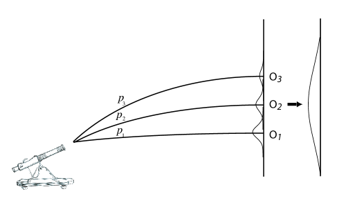
figure-images-covar-1\hyper@anchorend

We need a way to define the laboratory time which is independent of Alice or Bob.

We will do this not by finding a single laboratory time for the whole wave function, but by breaking the wave function into parts – for each of which we can find a reasonable laboratory time – propagating each part separately, and adding the parts back together at the end.

We work in the context of general relativity and think in terms of coordinate patches, small bits of space and time that are reasonably smooth. We will assume that our wave function is bounded within such a patch.

We need to have a way to deal with the extended character of the initial wave function and detector.

We break the wave function up into Morlet wavelets in four dimensions, so the full wave function is a sum over four dimensional Morlet wavelets, each of which is made of sixteen Gaussian test functions:

\Hy@raisedlink\hyper@anchorstartequationcovarcovar9\hyper@anchorendψ~sd=𝒟xAϕsd(xA)ψ(xA)\Hy@raisedlink\hyper@anchorstart𝑒𝑞𝑢𝑎𝑡𝑖𝑜𝑛𝑐𝑜𝑣𝑎𝑟𝑐𝑜𝑣𝑎𝑟9\hyper@anchorendsubscript~𝜓𝑠𝑑𝒟subscript𝑥𝐴superscriptsubscriptitalic-ϕ𝑠𝑑subscript𝑥𝐴𝜓subscript𝑥𝐴\Hy@raisedlink{\hyper@anchorstart{equation-covar-covar-9}\hyper@anchorend}{\tilde{\psi}}_{sd}={\displaystyle\int\mathcal{D}{x}_{A}{\phi}_{sd}^{\ast}\left({x}_{A}\right)\psi\left({x}_{A}\right)} (3.178)

For each wavelet, we have well-defined expectations for initial location:

\Hy@raisedlink\hyper@anchorstartequationcovarcovar9b\hyper@anchorendxμϕsd|xμ|ϕsdϕsd|ϕsd\Hy@raisedlink\hyper@anchorstart𝑒𝑞𝑢𝑎𝑡𝑖𝑜𝑛𝑐𝑜𝑣𝑎𝑟𝑐𝑜𝑣𝑎𝑟9𝑏\hyper@anchorenddelimited-⟨⟩superscript𝑥𝜇quantum-operator-productsubscriptitalic-ϕ𝑠𝑑superscript𝑥𝜇subscriptitalic-ϕ𝑠𝑑inner-productsubscriptitalic-ϕ𝑠𝑑subscriptitalic-ϕ𝑠𝑑\Hy@raisedlink{\hyper@anchorstart{equation-covar-covar-9b}\hyper@anchorend}\langle{x}^{\mu}\rangle\equiv\frac{\langle{\phi}_{sd}\left|{x}^{\mu}\right|{\phi}_{sd}\rangle}{\langle{\phi}_{sd}|{\phi}_{sd}\rangle} (3.179)

And initial momentum:

\Hy@raisedlink\hyper@anchorstartequationcovarcovar9d\hyper@anchorendpμiϕsd|xμ|ϕsdϕsd|ϕsd\Hy@raisedlink\hyper@anchorstart𝑒𝑞𝑢𝑎𝑡𝑖𝑜𝑛𝑐𝑜𝑣𝑎𝑟𝑐𝑜𝑣𝑎𝑟9𝑑\hyper@anchorendsuperscript𝑝𝜇𝑖quantum-operator-productsubscriptitalic-ϕ𝑠𝑑subscript𝑥𝜇subscriptitalic-ϕ𝑠𝑑inner-productsubscriptitalic-ϕ𝑠𝑑subscriptitalic-ϕ𝑠𝑑\Hy@raisedlink{\hyper@anchorstart{equation-covar-covar-9d}\hyper@anchorend}{p}^{\mu}\equiv i\frac{\langle{\phi}_{sd}\left|\frac{\partial}{\partial{x}_{\mu}}\right|{\phi}_{sd}\rangle}{\langle{\phi}_{sd}|{\phi}_{sd}\rangle} (3.180)

A well-defined initial position and momentum implies a well-defined classical trajectory. (We will assume that the detector is big enough that all such classical paths will hit it.)

The proper time along a classical trajectory is independent of the observer. This is our per wavelet laboratory time.

The kernel for each wavelet is now:

\Hy@raisedlink\hyper@anchorstartequationcovarcovarb\hyper@anchorendKΔτwaveletwavelet(xB;xA)=𝒟xwaveletexp(i𝐴𝐵dτwaveletL(x,dxdτwavelet))\Hy@raisedlink\hyper@anchorstart𝑒𝑞𝑢𝑎𝑡𝑖𝑜𝑛𝑐𝑜𝑣𝑎𝑟𝑐𝑜𝑣𝑎𝑟𝑏\hyper@anchorendsuperscriptsubscript𝐾Δsuperscript𝜏𝑤𝑎𝑣𝑒𝑙𝑒𝑡𝑤𝑎𝑣𝑒𝑙𝑒𝑡subscript𝑥𝐵subscript𝑥𝐴𝒟subscript𝑥𝑤𝑎𝑣𝑒𝑙𝑒𝑡exp𝑖𝐴𝐵dsubscript𝜏𝑤𝑎𝑣𝑒𝑙𝑒𝑡𝐿𝑥𝑑𝑥𝑑subscript𝜏𝑤𝑎𝑣𝑒𝑙𝑒𝑡\Hy@raisedlink{\hyper@anchorstart{equation-covar-covar-b}\hyper@anchorend}{K}_{\Delta{\tau}^{wavelet}}^{wavelet}\left({x}_{B};{x}_{A}\right)={\displaystyle\int\mathcal{D}{x}_{wavelet}\mathrm{exp}\left(i{\displaystyle\underset{A}{\overset{B}{\int}}\text{d}{\tau}_{wavelet}L\left(x,\frac{dx}{d{\tau}_{wavelet}}\right)}\right)} (3.181)

With the laboratory time now defined on a per wavelet basis, we have at the detector:

\Hy@raisedlink\hyper@anchorstartequationcovarcovarc\hyper@anchorendϕsd(xB)=dxAKΔτwaveletwavelet(xB;xA)ϕsd(xA)\Hy@raisedlink\hyper@anchorstart𝑒𝑞𝑢𝑎𝑡𝑖𝑜𝑛𝑐𝑜𝑣𝑎𝑟𝑐𝑜𝑣𝑎𝑟𝑐\hyper@anchorendsubscriptitalic-ϕ𝑠𝑑subscript𝑥𝐵dsubscript𝑥𝐴superscriptsubscript𝐾Δsuperscript𝜏𝑤𝑎𝑣𝑒𝑙𝑒𝑡𝑤𝑎𝑣𝑒𝑙𝑒𝑡subscript𝑥𝐵subscript𝑥𝐴subscriptitalic-ϕ𝑠𝑑subscript𝑥𝐴\Hy@raisedlink{\hyper@anchorstart{equation-covar-covar-c}\hyper@anchorend}{\phi}_{sd}\left({x}_{B}\right)={\displaystyle\int\text{d}{x}_{A}{K}_{\Delta{\tau}^{wavelet}}^{wavelet}\left({x}_{B};{x}_{A}\right){\phi}_{sd}\left({x}_{A}\right)} (3.182)

To get the full wave, we add the components up 101010 Because the laboratory time is now defined on a per wavelet basis, we can see the wavelets as being, in a certain sense, more fundamental than the full wave. :

\Hy@raisedlink\hyper@anchorstartequationcovarcovard\hyper@anchorendψ(xB)=𝒟s𝒟𝑑ϕsd(xB)ψ~sd\Hy@raisedlink\hyper@anchorstart𝑒𝑞𝑢𝑎𝑡𝑖𝑜𝑛𝑐𝑜𝑣𝑎𝑟𝑐𝑜𝑣𝑎𝑟𝑑\hyper@anchorend𝜓subscript𝑥𝐵𝒟𝑠𝒟differential-dsuperscriptsubscriptitalic-ϕ𝑠𝑑subscript𝑥𝐵subscript~𝜓𝑠𝑑\Hy@raisedlink{\hyper@anchorstart{equation-covar-covar-d}\hyper@anchorend}\psi\left({x}_{B}\right)={\displaystyle\int\mathcal{D}s\mathcal{D}d{\phi}_{sd}^{\ast}\left({x}_{B}\right){\tilde{\psi}}_{sd}} (3.183)

We have implicitly assumed that Alice and Bob can use the same wavelet decomposition. We have shown elsewhere ([96]) that we can define four dimensional Morlet wavelets in a covariant way; we will assume that Alice and Bob have read that paper and are willing to use that wavelet decomposition or an equivalent.

We will make use of this decomposition below in Slits in Time  when we analyze a wave function going through a gate.

3.7 Discussion

\Hy@raisedlink\hyper@anchorstart

tq-disc\hyper@anchorend

We have therefore satisfied our first two requirements: we needed only one but we have found four formalisms for temporal quantization which are well-defined and manifestly covariant.

We have also made some progress with respect to reasonably simple:

  1. 1.

    We have no need for factors of $i\epsilon$, Wick rotation, or the like. We get well-behaved path integrals, if we are careful to apply them to well-behaved functions.

  2. 2.

    And we have reasonably simple expressions for the Schrödinger equation:

    \Hy@raisedlink\hyper@anchorstartequationtqdisctqseqnderivseqn\hyper@anchorendidψτ(x)dτ=12m((peA)2m2)ψτ(x)\Hy@raisedlink\hyper@anchorstart𝑒𝑞𝑢𝑎𝑡𝑖𝑜𝑛𝑡𝑞𝑑𝑖𝑠𝑐𝑡𝑞𝑠𝑒𝑞𝑛𝑑𝑒𝑟𝑖𝑣𝑠𝑒𝑞𝑛\hyper@anchorend𝑖𝑑subscript𝜓𝜏𝑥𝑑𝜏12𝑚superscript𝑝𝑒𝐴2superscript𝑚2subscript𝜓𝜏𝑥\Hy@raisedlink{\hyper@anchorstart{equation-tq-disc-tq-seqn-deriv-seqn}\hyper@anchorend}i\frac{d{\psi}_{\tau}\left(x\right)}{d\tau}=-\frac{1}{2m}\left({\left(p-eA\right)}^{2}-{m}^{2}\right){\psi}_{\tau}\left(x\right) (3.184)
  3. 3.

    And its kernel:

    \Hy@raisedlink\hyper@anchorstartequationtqdisctqfpifinalfull\hyper@anchorendKτ(t,x′′;t,x)=(im24π2ϵ2)N+1n=1n=Nd4xnexp(i0𝜏L[tτ,xτ,dtτdτ,dxτdτ]dτ)\Hy@raisedlink\hyper@anchorstart𝑒𝑞𝑢𝑎𝑡𝑖𝑜𝑛𝑡𝑞𝑑𝑖𝑠𝑐𝑡𝑞𝑓𝑝𝑖𝑓𝑖𝑛𝑎𝑙𝑓𝑢𝑙𝑙\hyper@anchorendsubscript𝐾𝜏𝑡superscript𝑥′′𝑡superscript𝑥superscript𝑖superscript𝑚24superscript𝜋2superscriptitalic-ϵ2𝑁1superscriptsubscriptproduct𝑛1𝑛𝑁superscriptd4subscript𝑥𝑛exp𝑖0𝜏𝐿subscript𝑡𝜏subscript𝑥𝜏𝑑subscript𝑡𝜏𝑑𝜏𝑑subscript𝑥𝜏𝑑𝜏d𝜏\Hy@raisedlink{\hyper@anchorstart{equation-tq-disc-tq-fpi-final-full}\hyper@anchorend}{K}_{\tau}\left(t,{\overrightarrow{x}}^{{{}^{\prime\prime}}};t,{\overrightarrow{x}}^{\prime}\right)={\left(-\frac{i{m}^{2}}{4{\pi}^{2}{\epsilon}^{2}}\right)}^{N+1}{\displaystyle\int{\displaystyle\prod_{n=1}^{n=N}{\text{d}}^{\text{4}}{x}_{n}}\mathrm{exp}\left(i{\displaystyle\underset{0}{\overset{\tau}{\int}}L\left[{t}_{\tau},{\overrightarrow{x}}_{\tau},\frac{d{t}_{\tau}}{d\tau},\frac{d{\overrightarrow{x}}_{\tau}}{d\tau}\right]\text{d}\tau}\right)} (3.185)

Chapter 4 Comparison of Temporal Quantization To Standard Quantum Theory

\Hy@raisedlink\hyper@anchorstart

comp\hyper@anchorend

4.1 Overview

\Hy@raisedlink\hyper@anchorstart

comp-intro\hyper@anchorend

Quantum time functions as a fourth coordinate. It is like spin in being orthogonal to the other coordinates, unlike spin in being continuous and unbounded. Its properties are defined by covariance. Quantum time functions as a hidden coordinate – like a small mammal in the age of the dinosaurs, unlikely to be seen unless looked for – as spin did before the experiments of Stern and Gerlach ([456], [455], [454]).

If quantum time is real, why has it not been seen by chance? There are three reasons:

  1. 1.

    In terms of a classic beam/target experiment, unless both beam and target are varying in time, the effects of quantum time will tend to be averaged out.

  2. 2.

    Even if this is not the case, the principal effect of quantum time is increased dispersion in time. This is going to look like experimental noise, producing errors bars a bit wider in the time direction than might otherwise be the case. One seldom sees a headline in Science  or Nature  "Curiously large error bars seen in time measurement X".

  3. 3.

    In three limits, temporal quantization approaches standard quantum theory:

    1. (a)

      As the velocity goes to zero (Non-relativistic Limit).

    2. (b)

      As $\hslash$  goes to zero (Semi-classical Limit).

    3. (c)

      As we average over longer stretches of laboratory time (Long Time Limit).

We look at each of these three limits in turn.

4.2 Non-relativistic Limit

\Hy@raisedlink\hyper@anchorstart

nonrel\hyper@anchorend

We first look at the non-relativistic limit. We start with the path integral expression for the kernel:

\Hy@raisedlink\hyper@anchorstartequationnonrelnonsuch0\hyper@anchorendKτ(x′′;x)=𝒟xexp(i0𝜏dτ(m2(t˙2x˙2)+et˙Φ(t,x)ex˙A(t,x)+m2))\Hy@raisedlink\hyper@anchorstart𝑒𝑞𝑢𝑎𝑡𝑖𝑜𝑛𝑛𝑜𝑛𝑟𝑒𝑙𝑛𝑜𝑛𝑠𝑢𝑐0\hyper@anchorendsubscript𝐾𝜏superscript𝑥′′superscript𝑥𝒟𝑥exp𝑖0𝜏dsuperscript𝜏𝑚2superscript˙𝑡2superscript˙𝑥2𝑒˙𝑡Φ𝑡𝑥𝑒˙𝑥𝐴𝑡𝑥𝑚2\Hy@raisedlink{\hyper@anchorstart{equation-nonrel-nonsuch-0}\hyper@anchorend}{K}_{\tau}\left({x}^{{{}^{\prime\prime}}};{x}^{\prime}\right)={\displaystyle\int\mathcal{D}x\mathrm{exp}\left(-i{\displaystyle\underset{0}{\overset{\tau}{\int}}\text{d}{\tau}^{\prime}\left(\frac{m}{2}\left({\dot{t}}^{2}-{\dot{\overrightarrow{x}}}^{2}\right)+e\dot{t}\Phi\left(t,\overrightarrow{x}\right)-e\dot{\overrightarrow{x}}\cdot\overrightarrow{A}\left(t,\overrightarrow{x}\right)+\frac{m}{2}\right)}\right)} (4.1)

We expand the potentials around the laboratory time:

\Hy@raisedlink\hyper@anchorstartequationnonrelnonsuch1\hyper@anchorendA(t,x)=A(τ,x)+A(t,x)t|t=τtτ+122A(t,x)t2|t=τtτ2+\Hy@raisedlink\hyper@anchorstart𝑒𝑞𝑢𝑎𝑡𝑖𝑜𝑛𝑛𝑜𝑛𝑟𝑒𝑙𝑛𝑜𝑛𝑠𝑢𝑐1\hyper@anchorend𝐴𝑡𝑥𝐴𝜏𝑥evaluated-at𝐴𝑡𝑥𝑡𝑡𝜏subscript𝑡𝜏evaluated-at12superscript2𝐴𝑡𝑥superscript𝑡2𝑡𝜏superscriptsubscript𝑡𝜏2\Hy@raisedlink{\hyper@anchorstart{equation-nonrel-nonsuch-1}\hyper@anchorend}A\left(t,\overrightarrow{x}\right)=A\left(\tau,\overrightarrow{x}\right)+{\frac{\partial A\left(t,\overrightarrow{x}\right)}{\partial t}|}_{t=\tau}{t}_{\tau}+\frac{1}{2}{\frac{{\partial}^{2}A\left(t,\overrightarrow{x}\right)}{\partial{t}^{2}}|}_{t=\tau}{t}_{\tau}^{2}+\dots (4.2)

It is difficult to say much more in a general way about this without making some specific assumptions about the potentials. We now assume they are sufficiently slowly changing that the first and higher derivatives are negligible:

\Hy@raisedlink\hyper@anchorstartequationnonrelnonsuch2\hyper@anchorendA(t,x)A(τ,x)\Hy@raisedlink\hyper@anchorstart𝑒𝑞𝑢𝑎𝑡𝑖𝑜𝑛𝑛𝑜𝑛𝑟𝑒𝑙𝑛𝑜𝑛𝑠𝑢𝑐2\hyper@anchorend𝐴𝑡𝑥𝐴𝜏𝑥\Hy@raisedlink{\hyper@anchorstart{equation-nonrel-nonsuch-2}\hyper@anchorend}A\left(t,\overrightarrow{x}\right)\approx A\left(\tau,\overrightarrow{x}\right) (4.3)

The quantum time and standard quantum theory parts are entangled by the $e\dot{t}\Phi$  term. In the non-relativistic case, if we do the integrals by steepest descents (see below Semi-classical Limit), to lowest order the value of $\dot{t}$  will be replaced by its average, approximately one in the non-relativistic case:

\Hy@raisedlink\hyper@anchorstartequationnonrelnonrel1\hyper@anchorendt˙t˙1\Hy@raisedlink\hyper@anchorstart𝑒𝑞𝑢𝑎𝑡𝑖𝑜𝑛𝑛𝑜𝑛𝑟𝑒𝑙𝑛𝑜𝑛𝑟𝑒𝑙1\hyper@anchorend˙𝑡delimited-⟨⟩˙𝑡1\Hy@raisedlink{\hyper@anchorstart{equation-nonrel-nonrel-1}\hyper@anchorend}\dot{t}\rightarrow\langle\dot{t}\rangle\approx 1 (4.4)

This lets us separate the Lagrangian into a time part:

\Hy@raisedlink\hyper@anchorstartequationnonrelnonrel4b\hyper@anchorendLm2t˙2m2\Hy@raisedlink{\hyper@anchorstart{equation-nonrel-nonrel-4b}\hyper@anchorend}\stackrel{{\scriptstyle\frown}}{{L}}\equiv-\frac{m}{2}{\dot{t}}^{2}-\frac{m}{2} (4.5)

And a space part, the familiar ([403], [1017]):

\Hy@raisedlink\hyper@anchorstartequationnonrelnonrel5\hyper@anchorendL¯m2x˙2eΦ(τ,x)+ex˙A(τ,x)\Hy@raisedlink\hyper@anchorstart𝑒𝑞𝑢𝑎𝑡𝑖𝑜𝑛𝑛𝑜𝑛𝑟𝑒𝑙𝑛𝑜𝑛𝑟𝑒𝑙5\hyper@anchorend¯𝐿𝑚2superscript˙𝑥2𝑒Φ𝜏𝑥𝑒˙𝑥𝐴𝜏𝑥\Hy@raisedlink{\hyper@anchorstart{equation-nonrel-nonrel-5}\hyper@anchorend}\overline{L}\equiv\frac{m}{2}{\dot{\overrightarrow{x}}}^{2}-e\Phi\left(\tau,\overrightarrow{x}\right)+e\dot{\overrightarrow{x}}\cdot\overrightarrow{A}\left(\tau,\overrightarrow{x}\right) (4.6)

Giving:

\Hy@raisedlink\hyper@anchorstartequationnonrelnonrel4\hyper@anchorendLL+L¯\Hy@raisedlink{\hyper@anchorstart{equation-nonrel-nonrel-4}\hyper@anchorend}L\approx\stackrel{{\scriptstyle\frown}}{{L}}+\overline{L} (4.7)

We can factor the quantum time and space parts in the measure:

\Hy@raisedlink\hyper@anchorstartequationnonrelnonrel6\hyper@anchorend𝒟x=𝒟t𝒟x\Hy@raisedlink\hyper@anchorstart𝑒𝑞𝑢𝑎𝑡𝑖𝑜𝑛𝑛𝑜𝑛𝑟𝑒𝑙𝑛𝑜𝑛𝑟𝑒𝑙6\hyper@anchorend𝒟𝑥𝒟𝑡𝒟𝑥\Hy@raisedlink{\hyper@anchorstart{equation-nonrel-nonrel-6}\hyper@anchorend}\mathcal{D}x=\mathcal{D}t\mathcal{D}\overrightarrow{x} (4.8)

Using:

\Hy@raisedlink\hyper@anchorstartequationnonrelnonrel6b\hyper@anchorend𝒟tim2πϵNj=1Ndtj\Hy@raisedlink\hyper@anchorstart𝑒𝑞𝑢𝑎𝑡𝑖𝑜𝑛𝑛𝑜𝑛𝑟𝑒𝑙𝑛𝑜𝑛𝑟𝑒𝑙6𝑏\hyper@anchorend𝒟𝑡superscript𝑖𝑚2𝜋italic-ϵ𝑁superscriptsubscriptproductj=1Ndsubscript𝑡𝑗\Hy@raisedlink{\hyper@anchorstart{equation-nonrel-nonrel-6b}\hyper@anchorend}\mathcal{D}t\equiv{\sqrt{\frac{im}{2\pi\epsilon}}}^{N}{\displaystyle\prod_{\text{j=1}}^{\text{N}}\text{d}{t}_{j}} (4.9)
\Hy@raisedlink\hyper@anchorstartequationnonrelnonrel6c\hyper@anchorend𝒟xm2πiϵ3Nj=1Ndxj\Hy@raisedlink\hyper@anchorstart𝑒𝑞𝑢𝑎𝑡𝑖𝑜𝑛𝑛𝑜𝑛𝑟𝑒𝑙𝑛𝑜𝑛𝑟𝑒𝑙6𝑐\hyper@anchorend𝒟𝑥superscript𝑚2𝜋𝑖italic-ϵ3𝑁superscriptsubscriptproductj=1Ndsubscript𝑥𝑗\Hy@raisedlink{\hyper@anchorstart{equation-nonrel-nonrel-6c}\hyper@anchorend}\mathcal{D}\overrightarrow{x}\equiv{\sqrt{\frac{m}{2\pi i\epsilon}}}^{3N}{\displaystyle\prod_{\text{j=1}}^{\text{N}}\text{d}{\overrightarrow{x}}_{j}} (4.10)

And therefore we can factor the kernel:

\Hy@raisedlink\hyper@anchorstartequationnonrelnonrel7\hyper@anchorendKτ′′τ(x′′;x)Kτ′′τ(t′′;t)K¯τ′′τ(x′′;x)\Hy@raisedlink{\hyper@anchorstart{equation-nonrel-nonrel-7}\hyper@anchorend}{K}_{{\tau}^{{{}^{\prime\prime}}}{\tau}^{\prime}}\left({x}^{{{}^{\prime\prime}}};{x}^{\prime}\right)\approx{\stackrel{{\scriptstyle\frown}}{{K}}}_{{\tau}^{{{}^{\prime\prime}}}{\tau}^{\prime}}\left({t}^{{{}^{\prime\prime}}};{t}^{\prime}\right){\overline{K}}_{{\tau}^{{{}^{\prime\prime}}}{\tau}^{\prime}}\left({\overrightarrow{x}}^{{{}^{\prime\prime}}};{\overrightarrow{x}}^{\prime}\right) (4.11)

Into a time part:

\Hy@raisedlink\hyper@anchorstartequationnonrelnonrel7b\hyper@anchorendKτ′′τ(t′′;t)𝒟texp(iττ′′dτL)\Hy@raisedlink{\hyper@anchorstart{equation-nonrel-nonrel-7b}\hyper@anchorend}{\stackrel{{\scriptstyle\frown}}{{K}}}_{{\tau}^{{{}^{\prime\prime}}}{\tau}^{\prime}}\left({t}^{{{}^{\prime\prime}}};{t}^{\prime}\right)\equiv{\displaystyle\int\mathcal{D}t\mathrm{exp}\left(i{\displaystyle\underset{{\tau}^{\prime}}{\overset{{\tau}^{{{}^{\prime\prime}}}}{\int}}\text{d}\tau\stackrel{{\scriptstyle\frown}}{{L}}}\right)} (4.12)

And the familiar space (standard quantum theory) part:

\Hy@raisedlink\hyper@anchorstartequationnonrelnonrel7c\hyper@anchorendK¯τ′′τ(x′′;x)=𝒟xexp(iττ′′dτL¯)\Hy@raisedlink\hyper@anchorstart𝑒𝑞𝑢𝑎𝑡𝑖𝑜𝑛𝑛𝑜𝑛𝑟𝑒𝑙𝑛𝑜𝑛𝑟𝑒𝑙7𝑐\hyper@anchorendsubscript¯𝐾superscript𝜏′′superscript𝜏superscript𝑥′′superscript𝑥𝒟𝑥exp𝑖superscript𝜏superscript𝜏′′d𝜏¯𝐿\Hy@raisedlink{\hyper@anchorstart{equation-nonrel-nonrel-7c}\hyper@anchorend}{\overline{K}}_{{\tau}^{{{}^{\prime\prime}}}{\tau}^{\prime}}\left({\overrightarrow{x}}^{{{}^{\prime\prime}}};{\overrightarrow{x}}^{\prime}\right)={\displaystyle\int\mathcal{D}\overrightarrow{x}\mathrm{exp}\left(i{\displaystyle\underset{{\tau}^{\prime}}{\overset{{\tau}^{{{}^{\prime\prime}}}}{\int}}\text{d}\tau\overline{L}}\right)} (4.13)

Therefore we can separate the problem into a free quantum time part and the familiar standard quantum theory or space part if:

  1. 1.

    The velocities are non-relativistic,

  2. 2.

    And there is little or no time dependence in the potentials.

And therefore the final wave functions will be products of the free wave function in quantum time and the usual standard quantum theory wave function in space.

The free wave function in quantum time will have the effect of increasing the dispersion in time. If the initial dispersion in quantum time is small and the distances traveled short, the effects are likely to be small, easily written off as experimental noise.

4.3 Semi-classical Limit

\Hy@raisedlink\hyper@anchorstart

semi\hyper@anchorend

It is the outstanding feature of the path integral that the classical action of the system has appeared in a quantum mechanical expression, and it is this feature that is considered central to any extension of the path integral formalism.

— Mark Swanson [1101]

4.3.1 Overview

\Hy@raisedlink\hyper@anchorstart

semi-intro\hyper@anchorend

In the limit as $\hslash$  goes to zero we get the semi-classical approximation for standard quantum theory.

The semi-classical approximation for path integrals gives a clear connection to the classical picture: the classical trajectories mark the center of a quantum valley. The width of the quantum valley goes as $\hslash$, in the sense that as $\hslash$  goes to zero the quantum fluctuations vanish.

From this perspective, temporal quantization is to standard quantum theory as standard quantum theory is to classical mechanics; temporal quantization posits quantum fluctuations in time just as standard quantum theory posits quantum fluctuations in space.

We now examine the semi-classical approximation in temporal quantization. We use block time. We look at:

  1. 1.

    The Derivation of the Semi-classical Approximation;

  2. 2.

    Applications of the Semi-classical Approximation, specifically analyses of:

    1. (a)

      The Free Propagator,

    2. (b)

      Constant Potentials,

    3. (c)

      And the Constant Electric Field.

4.3.2 Derivation of the Semi-classical Approximation

\Hy@raisedlink\hyper@anchorstart

semi-calc\hyper@anchorend

To derive the semi-classical approximation, we rewrite the path integrals in terms of fluctuations around the classical path. We start with the path integral:

\Hy@raisedlink\hyper@anchorstartequationsemicalcsemicalc0\hyper@anchorendKτ(x′′;x)=CN+1dx1dx2dxNexp(iϵj=1j=N+1Lj)\Hy@raisedlink\hyper@anchorstart𝑒𝑞𝑢𝑎𝑡𝑖𝑜𝑛𝑠𝑒𝑚𝑖𝑐𝑎𝑙𝑐𝑠𝑒𝑚𝑖𝑐𝑎𝑙𝑐0\hyper@anchorendsubscript𝐾𝜏superscript𝑥′′superscript𝑥superscript𝐶𝑁1dsubscript𝑥1dsubscript𝑥2dsubscript𝑥𝑁exp𝑖italic-ϵsuperscriptsubscript𝑗1𝑗𝑁1subscript𝐿𝑗\Hy@raisedlink{\hyper@anchorstart{equation-semi-calc-semi-calc-0}\hyper@anchorend}{K}_{\tau}\left({x}^{{{}^{\prime\prime}}};{x}^{\prime}\right)={C}^{N+1}{\displaystyle\int\text{d}{x}_{1}\text{d}{x}_{2}\dots\text{d}{x}_{N}\mathrm{exp}\left(i\epsilon{\displaystyle\sum_{j=1}^{j=N+1}{L}_{j}}\right)} (4.14)

With:

\Hy@raisedlink\hyper@anchorstartequationsemicalcsemicalc1\hyper@anchorendLjm2(xjxj1ϵ)2exjxj1ϵ(A(xj)+A(xj1)2)m2\Hy@raisedlink\hyper@anchorstart𝑒𝑞𝑢𝑎𝑡𝑖𝑜𝑛𝑠𝑒𝑚𝑖𝑐𝑎𝑙𝑐𝑠𝑒𝑚𝑖𝑐𝑎𝑙𝑐1\hyper@anchorendsubscript𝐿𝑗𝑚2superscriptsubscript𝑥𝑗subscript𝑥𝑗1italic-ϵ2𝑒subscript𝑥𝑗subscript𝑥𝑗1italic-ϵ𝐴subscript𝑥𝑗𝐴subscript𝑥𝑗12𝑚2\Hy@raisedlink{\hyper@anchorstart{equation-semi-calc-semi-calc-1}\hyper@anchorend}{L}_{j}\equiv-\frac{m}{2}{\left(\frac{{x}_{j}-{x}_{j-1}}{\epsilon}\right)}^{2}-e\frac{{x}_{j}-{x}_{j-1}}{\epsilon}\left(\frac{A\left({x}_{j}\right)+A\left({x}_{j-1}\right)}{2}\right)-\frac{m}{2} (4.15)

We rewrite the coordinates as the classical solution plus the quantum variation from that ${x}_{j}={\overline{x}}_{j}+\delta{x}_{j}$. We set the first variation with respect to $\delta{x}_{j}^{\mu}$  to zero to get:

\Hy@raisedlink\hyper@anchorstartequationsemicalcsemicalc2\hyper@anchorendm(x¯jμx¯j1μϵ2)+m(x¯j+1μx¯jμϵ2)e2ϵ(Aμ(x¯j1)Aμ(x¯j+1))e2ϵ(x¯j+1νx¯j1ν)Aν(x¯j)xμj=0\Hy@raisedlink\hyper@anchorstart𝑒𝑞𝑢𝑎𝑡𝑖𝑜𝑛𝑠𝑒𝑚𝑖𝑐𝑎𝑙𝑐𝑠𝑒𝑚𝑖𝑐𝑎𝑙𝑐2\hyper@anchorend𝑚superscriptsubscript¯𝑥𝑗𝜇superscriptsubscript¯𝑥𝑗1𝜇superscriptitalic-ϵ2𝑚superscriptsubscript¯𝑥𝑗1𝜇superscriptsubscript¯𝑥𝑗𝜇superscriptitalic-ϵ2𝑒2italic-ϵsuperscript𝐴𝜇subscript¯𝑥𝑗1superscript𝐴𝜇subscript¯𝑥𝑗1𝑒2italic-ϵsuperscriptsubscript¯𝑥𝑗1𝜈superscriptsubscript¯𝑥𝑗1𝜈subscript𝐴𝜈subscript¯𝑥𝑗superscriptsubscript𝑥𝜇𝑗0\Hy@raisedlink{\hyper@anchorstart{equation-semi-calc-semi-calc-2}\hyper@anchorend}-m\left(\frac{{\overline{x}}_{j}^{\mu}-{\overline{x}}_{j-1}^{\mu}}{{\epsilon}^{2}}\right)+m\left(\frac{{\overline{x}}_{j+1}^{\mu}-{\overline{x}}_{j}^{\mu}}{{\epsilon}^{2}}\right)-\frac{e}{2\epsilon}\left({A}^{\mu}\left({\overline{x}}_{j-1}\right)-{A}^{\mu}\left({\overline{x}}_{j+1}\right)\right)-\frac{e}{2\epsilon}\left({\overline{x}}_{j+1}^{\nu}-{\overline{x}}_{j-1}^{\nu}\right)\frac{\partial{A}_{\nu}\left({\overline{x}}_{j}\right)}{\partial{x}_{\mu}^{j}}=0 (4.16)

In the continuum limit this is the classical equation of motion:

\Hy@raisedlink\hyper@anchorstartequationsemicalcsemicalc3\hyper@anchorendmx¨jμ=edAjμdτ+edxjνdτAν(xj)xμj=e(Aμ(xj)xνjAν(xj)xμj)dxjνdτ=eFνμ(xj)x˙jν\Hy@raisedlink\hyper@anchorstart𝑒𝑞𝑢𝑎𝑡𝑖𝑜𝑛𝑠𝑒𝑚𝑖𝑐𝑎𝑙𝑐𝑠𝑒𝑚𝑖𝑐𝑎𝑙𝑐3\hyper@anchorend𝑚superscriptsubscript¨𝑥𝑗𝜇𝑒𝑑superscriptsubscript𝐴𝑗𝜇𝑑𝜏𝑒𝑑superscriptsubscript𝑥𝑗𝜈𝑑𝜏subscript𝐴𝜈subscript𝑥𝑗superscriptsubscript𝑥𝜇𝑗𝑒superscript𝐴𝜇subscript𝑥𝑗superscriptsubscript𝑥𝜈𝑗subscript𝐴𝜈subscript𝑥𝑗superscriptsubscript𝑥𝜇𝑗𝑑superscriptsubscript𝑥𝑗𝜈𝑑𝜏𝑒superscriptsubscript𝐹𝜈𝜇subscript𝑥𝑗superscriptsubscript˙𝑥𝑗𝜈\Hy@raisedlink{\hyper@anchorstart{equation-semi-calc-semi-calc-3}\hyper@anchorend}m{\ddot{x}}_{j}^{\mu}=-e\frac{d{A}_{j}^{\mu}}{d\tau}+e\frac{d{x}_{j}^{\nu}}{d\tau}\frac{\partial{A}_{\nu}\left({x}_{j}\right)}{\partial{x}_{\mu}^{j}}=-e\left(\frac{\partial{A}^{\mu}\left({x}_{j}\right)}{\partial{x}_{\nu}^{j}}-\frac{\partial{A}_{\nu}\left({x}_{j}\right)}{\partial{x}_{\mu}^{j}}\right)\frac{d{x}_{j}^{\nu}}{d\tau}=e{F}_{\nu}^{\mu}\left({x}_{j}\right){\dot{x}}_{j}^{\nu} (4.17)

The full expression for the kernel is:

\Hy@raisedlink\hyper@anchorstartequationsemicalcsemicalc6\hyper@anchorendKτ(x′′;x)=dx1dx2dxNexp(iϵj=1j=N+1L¯j+122L¯jδxδxδxδx+O(δx)3)\Hy@raisedlink\hyper@anchorstart𝑒𝑞𝑢𝑎𝑡𝑖𝑜𝑛𝑠𝑒𝑚𝑖𝑐𝑎𝑙𝑐𝑠𝑒𝑚𝑖𝑐𝑎𝑙𝑐6\hyper@anchorendsubscript𝐾𝜏superscript𝑥′′superscript𝑥dsubscript𝑥1dsubscript𝑥2dsubscript𝑥𝑁exp𝑖italic-ϵsuperscriptsubscript𝑗1𝑗𝑁1subscript¯𝐿𝑗12superscript2subscript¯𝐿𝑗𝛿𝑥𝛿𝑥𝛿𝑥𝛿𝑥𝑂superscript𝛿𝑥3\Hy@raisedlink{\hyper@anchorstart{equation-semi-calc-semi-calc-6}\hyper@anchorend}{K}_{\tau}\left({x}^{{{}^{\prime\prime}}};{x}^{\prime}\right)={\displaystyle\int\text{d}{x}_{1}\text{d}{x}_{2}\dots\text{d}{x}_{N}\mathrm{exp}\left(i\epsilon{\displaystyle\sum_{j=1}^{j=N+1}{\overline{L}}_{j}+\frac{1}{2}\frac{{\partial}^{2}{\overline{L}}_{j}}{\partial\delta x\partial\delta x}\delta x\delta x+O{\left(\delta x\right)}^{3}}\right)} (4.18)

With:

\Hy@raisedlink\hyper@anchorstartequationsemicalcsemicalc7\hyper@anchorendL¯jm2(x¯jx¯j1ϵ)2ex¯jx¯j1ϵ(A(x¯j)+A(x¯j1)2)m2ϵ\Hy@raisedlink\hyper@anchorstart𝑒𝑞𝑢𝑎𝑡𝑖𝑜𝑛𝑠𝑒𝑚𝑖𝑐𝑎𝑙𝑐𝑠𝑒𝑚𝑖𝑐𝑎𝑙𝑐7\hyper@anchorendsubscript¯𝐿𝑗𝑚2superscriptsubscript¯𝑥𝑗subscript¯𝑥𝑗1italic-ϵ2𝑒subscript¯𝑥𝑗subscript¯𝑥𝑗1italic-ϵ𝐴subscript¯𝑥𝑗𝐴subscript¯𝑥𝑗12𝑚2italic-ϵ\Hy@raisedlink{\hyper@anchorstart{equation-semi-calc-semi-calc-7}\hyper@anchorend}{\overline{L}}_{j}\equiv-\frac{m}{2}{\left(\frac{{\overline{x}}_{j}-{\overline{x}}_{j-1}}{\epsilon}\right)}^{2}-e\frac{{\overline{x}}_{j}-{\overline{x}}_{j-1}}{\epsilon}\left(\frac{A\left({\overline{x}}_{j}\right)+A\left({\overline{x}}_{j-1}\right)}{2}\right)-\frac{m}{2}\epsilon (4.19)

This is exact when we include the cubic and higher terms. Including only terms through the quadratic we get:

\Hy@raisedlink\hyper@anchorstartequationsemicalcsemicalc8\hyper@anchorendKτ(x′′;x)Fτ(x′′;x)K¯τ(x′′;x)\Hy@raisedlink\hyper@anchorstart𝑒𝑞𝑢𝑎𝑡𝑖𝑜𝑛𝑠𝑒𝑚𝑖𝑐𝑎𝑙𝑐𝑠𝑒𝑚𝑖𝑐𝑎𝑙𝑐8\hyper@anchorendsubscript𝐾𝜏superscript𝑥′′superscript𝑥subscript𝐹𝜏superscript𝑥′′superscript𝑥subscript¯𝐾𝜏superscript𝑥′′superscript𝑥\Hy@raisedlink{\hyper@anchorstart{equation-semi-calc-semi-calc-8}\hyper@anchorend}{K}_{\tau}\left({x}^{{{}^{\prime\prime}}};{x}^{\prime}\right)\approx{F}_{\tau}\left({x}^{{{}^{\prime\prime}}};{x}^{\prime}\right){\overline{K}}_{\tau}\left({x}^{{{}^{\prime\prime}}};{x}^{\prime}\right) (4.20)

With:

\Hy@raisedlink\hyper@anchorstartequationsemicalcsemicalc5\hyper@anchorendK¯τ(x′′;x)=exp(iϵj=1j=N+1L¯j)\Hy@raisedlink\hyper@anchorstart𝑒𝑞𝑢𝑎𝑡𝑖𝑜𝑛𝑠𝑒𝑚𝑖𝑐𝑎𝑙𝑐𝑠𝑒𝑚𝑖𝑐𝑎𝑙𝑐5\hyper@anchorendsubscript¯𝐾𝜏superscript𝑥′′superscript𝑥exp𝑖italic-ϵsuperscriptsubscript𝑗1𝑗𝑁1subscript¯𝐿𝑗\Hy@raisedlink{\hyper@anchorstart{equation-semi-calc-semi-calc-5}\hyper@anchorend}{\overline{K}}_{\tau}\left({x}^{{{}^{\prime\prime}}};{x}^{\prime}\right)=\mathrm{exp}\left(i\epsilon{\displaystyle\sum_{j=1}^{j=N+1}{\overline{L}}_{j}}\right) (4.21)

And fluctuation factor F:

\Hy@raisedlink\hyper@anchorstartequationsemicalcsemicalc9\hyper@anchorendFτ(x′′;x)CN+1dδx1dδx2dδxNexp(iϵj=1j=N+1122L¯jδxμδxνδxμδxν)\Hy@raisedlink\hyper@anchorstart𝑒𝑞𝑢𝑎𝑡𝑖𝑜𝑛𝑠𝑒𝑚𝑖𝑐𝑎𝑙𝑐𝑠𝑒𝑚𝑖𝑐𝑎𝑙𝑐9\hyper@anchorendsubscript𝐹𝜏superscript𝑥′′superscript𝑥superscript𝐶𝑁1d𝛿subscript𝑥1d𝛿subscript𝑥2d𝛿subscript𝑥𝑁exp𝑖italic-ϵsuperscriptsubscript𝑗1𝑗𝑁112superscript2subscript¯𝐿𝑗𝛿superscript𝑥𝜇𝛿superscript𝑥𝜈𝛿superscript𝑥𝜇𝛿superscript𝑥𝜈\Hy@raisedlink{\hyper@anchorstart{equation-semi-calc-semi-calc-9}\hyper@anchorend}{F}_{\tau}\left({x}^{{{}^{\prime\prime}}};{x}^{\prime}\right)\equiv{C}^{N+1}{\displaystyle\int\text{d}\delta{x}_{1}\text{d}\delta{x}_{2}\dots\text{d}\delta{x}_{N}\mathrm{exp}\left(i\epsilon{\displaystyle\sum_{j=1}^{j=N+1}\frac{1}{2}\frac{{\partial}^{2}{\overline{L}}_{j}}{\partial\delta{x}^{\mu}\partial\delta{x}^{\nu}}\delta{x}^{\mu}\delta{x}^{\nu}}\right)} (4.22)

The fluctuation factor can be computed in terms of the action and its derivatives. The derivation is nontrivial. It is treated in the one dimensional case in [1017]  and in one dimensional and higher dimensions in [672]  and [694].

To extend these derivations to apply to the four dimensional case we need to:

  1. 1.

    Go from three to four dimensions,

  2. 2.

    And rely on Morlet wavelets, not factors of $i\epsilon$  or Wick rotation, for convergence.

Neither of these changes has any material impact on the derivations. Therefore the result is the same in temporal quantization as in standard quantum theory:

\Hy@raisedlink\hyper@anchorstartequationsemicalcsemicalcffsca\hyper@anchorendKτ(x′′;x)12πi4det(2Sτ(x′′;x)xx′′)exp(iSτ(x′′;x))\Hy@raisedlink\hyper@anchorstart𝑒𝑞𝑢𝑎𝑡𝑖𝑜𝑛𝑠𝑒𝑚𝑖𝑐𝑎𝑙𝑐𝑠𝑒𝑚𝑖𝑐𝑎𝑙𝑐𝑓𝑓𝑠𝑐𝑎\hyper@anchorendsubscript𝐾𝜏superscript𝑥′′superscript𝑥1superscript2𝜋𝑖4detsuperscript2subscript𝑆𝜏superscript𝑥′′superscript𝑥superscript𝑥superscript𝑥′′exp𝑖subscript𝑆𝜏superscript𝑥′′superscript𝑥\Hy@raisedlink{\hyper@anchorstart{equation-semi-calc-semi-calc-ff-sca}\hyper@anchorend}{K}_{\tau}\left({x}^{{{}^{\prime\prime}}};{x}^{\prime}\right)\approx\frac{1}{{\sqrt{2\pi i}}^{4}}\sqrt{\mathrm{det}\left(-\frac{{\partial}^{2}{S}_{\tau}\left({x}^{{{}^{\prime\prime}}};{x}^{\prime}\right)}{\partial{x}^{\prime}\partial{x}^{{{}^{\prime\prime}}}}\right)}\mathrm{exp}\left(i{S}_{\tau}\left({x}^{{{}^{\prime\prime}}};{x}^{\prime}\right)\right) (4.23)

We assume that the action is taken along the classical trajectory from ${x}^{\prime}$  to ${x}^{{{}^{\prime\prime}}}$and that the determinant has not passed through a singularity on this trajectory. We will verify this for several cases.

4.3.3 Applications of the Semi-classical Approximation

\Hy@raisedlink\hyper@anchorstart

semi-apps\hyper@anchorend

The semi-classical approximation is exact for Lagrangians no worse than quadratic in the coordinates. We look at three cases:

  1. 1.

    The Free Propagator,

  2. 2.

    Constant Potentials,

  3. 3.

    And the Constant Electric Field.

4.3.3.1 Free Propagator
\Hy@raisedlink\hyper@anchorstart

semi-free\hyper@anchorend

Free Propagator

The calculation of the free propagator in the semi-classical approximation provides a useful check. The Lagrangian is:

\Hy@raisedlink\hyper@anchorstartequationsemifreesemifree0\hyper@anchorendL(x,x˙)=m2x˙2m2\Hy@raisedlink\hyper@anchorstart𝑒𝑞𝑢𝑎𝑡𝑖𝑜𝑛𝑠𝑒𝑚𝑖𝑓𝑟𝑒𝑒𝑠𝑒𝑚𝑖𝑓𝑟𝑒𝑒0\hyper@anchorendL𝑥˙𝑥𝑚2superscript˙𝑥2𝑚2\Hy@raisedlink{\hyper@anchorstart{equation-semi-free-semi-free-0}\hyper@anchorend}\text{L}\left(x,\dot{x}\right)=-\frac{m}{2}{\dot{x}}^{2}-\frac{m}{2} (4.24)

The Euler-Lagrange   equations give:

\Hy@raisedlink\hyper@anchorstartequationsemifreesemifree1\hyper@anchorendmx¨=0\Hy@raisedlink\hyper@anchorstart𝑒𝑞𝑢𝑎𝑡𝑖𝑜𝑛𝑠𝑒𝑚𝑖𝑓𝑟𝑒𝑒𝑠𝑒𝑚𝑖𝑓𝑟𝑒𝑒1\hyper@anchorend𝑚¨𝑥0\Hy@raisedlink{\hyper@anchorstart{equation-semi-free-semi-free-1}\hyper@anchorend}m\ddot{x}=0 (4.25)

The classical trajectory is a straight line:

\Hy@raisedlink\hyper@anchorstartequationsemifreesemifree2\hyper@anchorendxτ=x′′xττ+x\Hy@raisedlink\hyper@anchorstart𝑒𝑞𝑢𝑎𝑡𝑖𝑜𝑛𝑠𝑒𝑚𝑖𝑓𝑟𝑒𝑒𝑠𝑒𝑚𝑖𝑓𝑟𝑒𝑒2\hyper@anchorendsubscript𝑥superscript𝜏superscript𝑥′′superscript𝑥𝜏superscript𝜏superscript𝑥\Hy@raisedlink{\hyper@anchorstart{equation-semi-free-semi-free-2}\hyper@anchorend}{x}_{{\tau}^{\prime}}=\frac{{x}^{{{}^{\prime\prime}}}-{x}^{\prime}}{\tau}{\tau}^{\prime}+{x}^{\prime} (4.26)

The Lagrangian on the classical trajectory is constant:

\Hy@raisedlink\hyper@anchorstartequationsemifreesemifree3\hyper@anchorendL=m2(Δxτ)2m2\Hy@raisedlink\hyper@anchorstart𝑒𝑞𝑢𝑎𝑡𝑖𝑜𝑛𝑠𝑒𝑚𝑖𝑓𝑟𝑒𝑒𝑠𝑒𝑚𝑖𝑓𝑟𝑒𝑒3\hyper@anchorend𝐿𝑚2superscriptΔ𝑥𝜏2𝑚2\Hy@raisedlink{\hyper@anchorstart{equation-semi-free-semi-free-3}\hyper@anchorend}L=-\frac{m}{2}{\left(\frac{\Delta x}{\tau}\right)}^{2}-\frac{m}{2} (4.27)

The action is:

\Hy@raisedlink\hyper@anchorstartequationsemifreesemifree4\hyper@anchorendS=m2τ(Δx)2m2τ\Hy@raisedlink\hyper@anchorstart𝑒𝑞𝑢𝑎𝑡𝑖𝑜𝑛𝑠𝑒𝑚𝑖𝑓𝑟𝑒𝑒𝑠𝑒𝑚𝑖𝑓𝑟𝑒𝑒4\hyper@anchorend𝑆𝑚2𝜏superscriptΔ𝑥2𝑚2𝜏\Hy@raisedlink{\hyper@anchorstart{equation-semi-free-semi-free-4}\hyper@anchorend}S=-\frac{m}{2\tau}{\left(\Delta x\right)}^{2}-\frac{m}{2}\tau (4.28)

The determinant of the action is:

\Hy@raisedlink\hyper@anchorstartequationsemifreesemifree5\hyper@anchorenddet(2S(x′′;x)x′′x)=m4τ4\Hy@raisedlink\hyper@anchorstart𝑒𝑞𝑢𝑎𝑡𝑖𝑜𝑛𝑠𝑒𝑚𝑖𝑓𝑟𝑒𝑒𝑠𝑒𝑚𝑖𝑓𝑟𝑒𝑒5\hyper@anchorenddetsuperscript2𝑆superscript𝑥′′superscript𝑥superscript𝑥′′superscript𝑥superscript𝑚4superscript𝜏4\Hy@raisedlink{\hyper@anchorstart{equation-semi-free-semi-free-5}\hyper@anchorend}\mathrm{det}\left(-\frac{{\partial}^{2}S\left({x}^{{{}^{\prime\prime}}};{x}^{\prime}\right)}{\partial{x}^{{{}^{\prime\prime}}}\partial{x}^{\prime}}\right)=-\frac{{m}^{4}}{{\tau}^{4}} (4.29)

And the kernel is:

\Hy@raisedlink\hyper@anchorstartequationsemifreefreefourtkernel\hyper@anchorendKτ(x′′;x)=im24π2τ2exp(im2τ(x′′x)2im2τ)\Hy@raisedlink\hyper@anchorstart𝑒𝑞𝑢𝑎𝑡𝑖𝑜𝑛𝑠𝑒𝑚𝑖𝑓𝑟𝑒𝑒𝑓𝑟𝑒𝑒𝑓𝑜𝑢𝑟𝑡𝑘𝑒𝑟𝑛𝑒𝑙\hyper@anchorendsubscript𝐾𝜏superscript𝑥′′superscript𝑥𝑖superscript𝑚24superscript𝜋2superscript𝜏2exp𝑖𝑚2𝜏superscriptsuperscript𝑥′′superscript𝑥2𝑖𝑚2𝜏\Hy@raisedlink{\hyper@anchorstart{equation-semi-free-free-fourt-kernel}\hyper@anchorend}{K}_{\tau}\left({x}^{{{}^{\prime\prime}}};{x}^{\prime}\right)=-\frac{i{m}^{2}}{4{\pi}^{2}{\tau}^{2}}\mathrm{exp}\left(-\frac{im}{2\tau}{\left({x}^{{{}^{\prime\prime}}}-{x}^{\prime}\right)}^{2}-i\frac{m}{2}\tau\right) (4.30)

This agrees with the free kernel derived in Feynman Path Integrals.

4.3.3.2 Constant Potentials
\Hy@raisedlink\hyper@anchorstart

semi-const\hyper@anchorend

Now we look at the case when the electric potential and vector potential are assumed constant:

\Hy@raisedlink\hyper@anchorstartequationsemiconstsemiconst3\hyper@anchorendA=(Φ,A)\Hy@raisedlink\hyper@anchorstart𝑒𝑞𝑢𝑎𝑡𝑖𝑜𝑛𝑠𝑒𝑚𝑖𝑐𝑜𝑛𝑠𝑡𝑠𝑒𝑚𝑖𝑐𝑜𝑛𝑠𝑡3\hyper@anchorend𝐴Φ𝐴\Hy@raisedlink{\hyper@anchorstart{equation-semi-const-semi-const-3}\hyper@anchorend}A=\left(\Phi,\overrightarrow{A}\right) (4.31)

The Lagrangian is:

\Hy@raisedlink\hyper@anchorstartequationsemiconstsemiconst0\hyper@anchorendL(x,dxdτ)=m2t˙2+m2x˙2et˙Φ+ex˙Am2\Hy@raisedlink\hyper@anchorstart𝑒𝑞𝑢𝑎𝑡𝑖𝑜𝑛𝑠𝑒𝑚𝑖𝑐𝑜𝑛𝑠𝑡𝑠𝑒𝑚𝑖𝑐𝑜𝑛𝑠𝑡0\hyper@anchorend𝐿𝑥𝑑𝑥𝑑𝜏𝑚2superscript˙𝑡2𝑚2superscript˙𝑥2𝑒˙𝑡Φ𝑒˙𝑥𝐴𝑚2\Hy@raisedlink{\hyper@anchorstart{equation-semi-const-semi-const-0}\hyper@anchorend}L\left(x,\frac{dx}{d\tau}\right)=-\frac{m}{2}{\dot{t}}^{2}+\frac{m}{2}{\dot{\overrightarrow{x}}}^{2}-e\dot{t}\Phi+e\dot{\overrightarrow{x}}\cdot\overrightarrow{A}-\frac{m}{2} (4.32)

The equations of motion are unchanged.

The action is the free action plus $\Delta S$:

\Hy@raisedlink\hyper@anchorstartequationsemiconstsemiconst1\hyper@anchorendΔS=e0𝜏dτΔtτΦΔxτA=eΔtΦ+eΔxA\Hy@raisedlink\hyper@anchorstart𝑒𝑞𝑢𝑎𝑡𝑖𝑜𝑛𝑠𝑒𝑚𝑖𝑐𝑜𝑛𝑠𝑡𝑠𝑒𝑚𝑖𝑐𝑜𝑛𝑠𝑡1\hyper@anchorendΔ𝑆𝑒0𝜏dsuperscript𝜏Δ𝑡𝜏ΦΔ𝑥𝜏𝐴𝑒Δ𝑡Φ𝑒Δ𝑥𝐴\Hy@raisedlink{\hyper@anchorstart{equation-semi-const-semi-const-1}\hyper@anchorend}\Delta S=-e{\displaystyle\underset{0}{\overset{\tau}{\int}}\text{d}{\tau}^{\prime}}\frac{\Delta t}{\tau}\Phi-\frac{\Delta\overrightarrow{x}}{\tau}\cdot\overrightarrow{A}=-e\Delta t\Phi+e\Delta\overrightarrow{x}\cdot\overrightarrow{A} (4.33)

The determinant of the action and therefore the fluctuation factor is unaffected. The kernel gets a change of phase:

\Hy@raisedlink\hyper@anchorstartequationsemiconstsemiconst2\hyper@anchorendKτ(const)(x′′;x)=Kτ(free)(x′′;x)exp(ieΔtΦ+ieΔxA)\Hy@raisedlink\hyper@anchorstart𝑒𝑞𝑢𝑎𝑡𝑖𝑜𝑛𝑠𝑒𝑚𝑖𝑐𝑜𝑛𝑠𝑡𝑠𝑒𝑚𝑖𝑐𝑜𝑛𝑠𝑡2\hyper@anchorendsuperscriptsubscript𝐾𝜏𝑐𝑜𝑛𝑠𝑡superscript𝑥′′superscript𝑥superscriptsubscript𝐾𝜏𝑓𝑟𝑒𝑒superscript𝑥′′superscript𝑥exp𝑖𝑒Δ𝑡Φ𝑖𝑒Δ𝑥𝐴\Hy@raisedlink{\hyper@anchorstart{equation-semi-const-semi-const-2}\hyper@anchorend}{K}_{\tau}^{\left(const\right)}\left({x}^{{{}^{\prime\prime}}};{x}^{\prime}\right)={K}_{\tau}^{\left(free\right)}\left({x}^{{{}^{\prime\prime}}};{x}^{\prime}\right)\mathrm{exp}\left(-ie\Delta t\Phi+ie\Delta\overrightarrow{x}\cdot\overrightarrow{A}\right) (4.34)

This is essentially a gauge change, with the choice of gauge:

\Hy@raisedlink\hyper@anchorstartequationsemiconstsemiconst4\hyper@anchorendΛτ(t,x)=xμAμ\Hy@raisedlink\hyper@anchorstart𝑒𝑞𝑢𝑎𝑡𝑖𝑜𝑛𝑠𝑒𝑚𝑖𝑐𝑜𝑛𝑠𝑡𝑠𝑒𝑚𝑖𝑐𝑜𝑛𝑠𝑡4\hyper@anchorendsubscriptΛ𝜏𝑡𝑥subscript𝑥𝜇superscript𝐴𝜇\Hy@raisedlink{\hyper@anchorstart{equation-semi-const-semi-const-4}\hyper@anchorend}{\Lambda}_{\tau}\left(t,\overrightarrow{x}\right)=-{x}_{\mu}{A}^{\mu} (4.35)

For a single trajectory, this has no more impact on probabilities than any other gauge change would have.

However, if there are two (or more) classical trajectories from source to detector, different phase changes along the different paths may result in interference patterns at the detector. See the Aharonov-Bohm Experiment  below.

4.3.3.3 Constant Electric Field
\Hy@raisedlink\hyper@anchorstart

semi-elec\hyper@anchorend

Now we look at the case of a constant electric field.

This is formally similar to that of the constant magnetic field, under interchange of x  and $t$:

\Hy@raisedlink\hyper@anchorstartequationsemielecsemielecflip0\hyper@anchorendxytxEB\Hy@raisedlink\hyper@anchorstart𝑒𝑞𝑢𝑎𝑡𝑖𝑜𝑛𝑠𝑒𝑚𝑖𝑒𝑙𝑒𝑐𝑠𝑒𝑚𝑖𝑒𝑙𝑒𝑐𝑓𝑙𝑖𝑝0\hyper@anchorend𝑥𝑦𝑡𝑥𝐸𝐵\Hy@raisedlink{\hyper@anchorstart{equation-semi-elec-semi-elec-flip-0}\hyper@anchorend}\begin{array}[]{l}x\rightarrow y\\ t\rightarrow x\\ \overrightarrow{E}\rightarrow\overrightarrow{B}\end{array} (4.36)

The treatment here is modeled on the treatment of the constant magnetic field in [694]. To emphasize the similarities, we assume we have gauged away the $-m/2$  term in the Lagrangian (Gauge Transformations for the Schrödinger Equation).

Derivation of Kernel

We focus on the $t$  and x  dimensions. We take the electric field along the x  direction:

\Hy@raisedlink\hyper@anchorstartequationsemielecsemielec0\hyper@anchorendE=Ex^\Hy@raisedlink\hyper@anchorstart𝑒𝑞𝑢𝑎𝑡𝑖𝑜𝑛𝑠𝑒𝑚𝑖𝑒𝑙𝑒𝑐𝑠𝑒𝑚𝑖𝑒𝑙𝑒𝑐0\hyper@anchorend𝐸𝐸^𝑥\Hy@raisedlink{\hyper@anchorstart{equation-semi-elec-semi-elec-0}\hyper@anchorend}\overrightarrow{E}=E\widehat{x} (4.37)

We choose the four-potential to be in Lorentz gauge and symmetric between $t$  and x:

\Hy@raisedlink\hyper@anchorstartequationsemielecsemielec1\hyper@anchorendA=E2(x,t,0,0)\Hy@raisedlink\hyper@anchorstart𝑒𝑞𝑢𝑎𝑡𝑖𝑜𝑛𝑠𝑒𝑚𝑖𝑒𝑙𝑒𝑐𝑠𝑒𝑚𝑖𝑒𝑙𝑒𝑐1\hyper@anchorend𝐴𝐸2𝑥𝑡00\Hy@raisedlink{\hyper@anchorstart{equation-semi-elec-semi-elec-1}\hyper@anchorend}A=\frac{E}{2}\left(-x,-t,0,0\right) (4.38)

This gives the Lagrangian:

\Hy@raisedlink\hyper@anchorstartequationsemielecsemielec2\hyper@anchorendL=m2t˙2+m2x˙2+eE2xt˙eE2tx˙\Hy@raisedlink\hyper@anchorstart𝑒𝑞𝑢𝑎𝑡𝑖𝑜𝑛𝑠𝑒𝑚𝑖𝑒𝑙𝑒𝑐𝑠𝑒𝑚𝑖𝑒𝑙𝑒𝑐2\hyper@anchorend𝐿𝑚2superscript˙𝑡2𝑚2superscript˙𝑥2𝑒𝐸2𝑥˙𝑡𝑒𝐸2𝑡˙𝑥\Hy@raisedlink{\hyper@anchorstart{equation-semi-elec-semi-elec-2}\hyper@anchorend}L=-\frac{m}{2}{\dot{t}}^{2}+\frac{m}{2}{\dot{\overrightarrow{x}}}^{2}+\frac{eE}{2}x\dot{t}-\frac{eE}{2}t\dot{x} (4.39)

And the Euler-Lagrange   equations:

\Hy@raisedlink\hyper@anchorstartequationsemielecsemielec3\hyper@anchorendt¨=αx˙x¨=αt˙\Hy@raisedlink\hyper@anchorstart𝑒𝑞𝑢𝑎𝑡𝑖𝑜𝑛𝑠𝑒𝑚𝑖𝑒𝑙𝑒𝑐𝑠𝑒𝑚𝑖𝑒𝑙𝑒𝑐3\hyper@anchorend¨𝑡𝛼˙𝑥¨𝑥𝛼˙𝑡\Hy@raisedlink{\hyper@anchorstart{equation-semi-elec-semi-elec-3}\hyper@anchorend}\begin{array}[]{l}\ddot{t}=\alpha\dot{x}\\ \ddot{x}=\alpha\dot{t}\end{array} (4.40)

Defining $\alpha\equiv eE/m$, the action for x  and $t$  is:

\Hy@raisedlink\hyper@anchorstartequationsemielecsemielec5\hyper@anchorendSτ′′τ(elec)=m20𝜏dτ(t˙2+x˙2+αt˙xαtx˙)\Hy@raisedlink\hyper@anchorstart𝑒𝑞𝑢𝑎𝑡𝑖𝑜𝑛𝑠𝑒𝑚𝑖𝑒𝑙𝑒𝑐𝑠𝑒𝑚𝑖𝑒𝑙𝑒𝑐5\hyper@anchorendsuperscriptsubscript𝑆superscript𝜏′′superscript𝜏𝑒𝑙𝑒𝑐𝑚20𝜏dsuperscript𝜏superscript˙𝑡2superscript˙𝑥2𝛼˙𝑡𝑥𝛼𝑡˙𝑥\Hy@raisedlink{\hyper@anchorstart{equation-semi-elec-semi-elec-5}\hyper@anchorend}{S}_{{\tau}^{{{}^{\prime\prime}}}{\tau}^{\prime}}^{\left(elec\right)}=\frac{m}{2}{\displaystyle\underset{0}{\overset{\tau}{\int}}\text{d}{\tau}^{\prime}\left(-{\dot{t}}^{2}+{\dot{x}}^{2}+\alpha\dot{t}x-\alpha t\dot{x}\right)} (4.41)

Integrating by parts we get:

\Hy@raisedlink\hyper@anchorstartequationsemielecsemielec6\hyper@anchorendSτ′′τ(elec)=m2(tt˙+xx˙)|ττ′′+m2ττ′′dτ(tt¨xx¨+αt˙xαtx˙)\Hy@raisedlink\hyper@anchorstart𝑒𝑞𝑢𝑎𝑡𝑖𝑜𝑛𝑠𝑒𝑚𝑖𝑒𝑙𝑒𝑐𝑠𝑒𝑚𝑖𝑒𝑙𝑒𝑐6\hyper@anchorendsuperscriptsubscript𝑆superscript𝜏′′superscript𝜏𝑒𝑙𝑒𝑐evaluated-at𝑚2𝑡˙𝑡𝑥˙𝑥superscript𝜏superscript𝜏′′𝑚2superscript𝜏superscript𝜏′′d𝜏𝑡¨𝑡𝑥¨𝑥𝛼˙𝑡𝑥𝛼𝑡˙𝑥\Hy@raisedlink{\hyper@anchorstart{equation-semi-elec-semi-elec-6}\hyper@anchorend}{S}_{{\tau}^{{{}^{\prime\prime}}}{\tau}^{\prime}}^{\left(elec\right)}=\frac{m}{2}{\left(-t\dot{t}+x\dot{x}\right)|}_{{\tau}^{\prime}}^{{\tau}^{{{}^{\prime\prime}}}}+\frac{m}{2}{\displaystyle\underset{{\tau}^{\prime}}{\overset{{\tau}^{{{}^{\prime\prime}}}}{\int}}\text{d}\tau\left(t\ddot{t}-x\ddot{x}+\alpha\dot{t}x-\alpha t\dot{x}\right)} (4.42)

From the equations of motion the integral is zero. Therefore the action is:

\Hy@raisedlink\hyper@anchorstartequationsemielecsemielec7\hyper@anchorendSτ′′τ(elec)=m2(tt˙+xx˙)|ττ′′=m2(t′′t˙′′+tt˙+x′′x˙′′xx˙)\Hy@raisedlink\hyper@anchorstart𝑒𝑞𝑢𝑎𝑡𝑖𝑜𝑛𝑠𝑒𝑚𝑖𝑒𝑙𝑒𝑐𝑠𝑒𝑚𝑖𝑒𝑙𝑒𝑐7\hyper@anchorendsuperscriptsubscript𝑆superscript𝜏′′superscript𝜏𝑒𝑙𝑒𝑐evaluated-at𝑚2𝑡˙𝑡𝑥˙𝑥superscript𝜏superscript𝜏′′𝑚2superscript𝑡′′superscript˙𝑡′′superscript𝑡superscript˙𝑡superscript𝑥′′superscript˙𝑥′′superscript𝑥superscript˙𝑥\Hy@raisedlink{\hyper@anchorstart{equation-semi-elec-semi-elec-7}\hyper@anchorend}{S}_{{\tau}^{{{}^{\prime\prime}}}{\tau}^{\prime}}^{\left(elec\right)}=\frac{m}{2}{\left(-t\dot{t}+x\dot{x}\right)|}_{{\tau}^{\prime}}^{{\tau}^{{{}^{\prime\prime}}}}=\frac{m}{2}\left(-{t}^{{{}^{\prime\prime}}}{\dot{t}}^{{{}^{\prime\prime}}}+{t}^{\prime}{\dot{t}}^{\prime}+{x}^{{{}^{\prime\prime}}}{\dot{x}}^{{{}^{\prime\prime}}}-{x}^{\prime}{\dot{x}}^{\prime}\right) (4.43)

We take the derivative of both sides of the Euler-Lagrange   equations with respect to laboratory time:

\Hy@raisedlink\hyper@anchorstartequationsemielecsemielec8\hyper@anchorendt¨˙=α2t˙x¨˙=α2x˙\Hy@raisedlink\hyper@anchorstart𝑒𝑞𝑢𝑎𝑡𝑖𝑜𝑛𝑠𝑒𝑚𝑖𝑒𝑙𝑒𝑐𝑠𝑒𝑚𝑖𝑒𝑙𝑒𝑐8\hyper@anchorend˙¨𝑡superscript𝛼2˙𝑡˙¨𝑥superscript𝛼2˙𝑥\Hy@raisedlink{\hyper@anchorstart{equation-semi-elec-semi-elec-8}\hyper@anchorend}\begin{array}[]{l}\dot{\ddot{t}}={\alpha}^{2}\dot{t}\\ \dot{\ddot{x}}={\alpha}^{2}\dot{x}\end{array} (4.44)

The solutions are:

\Hy@raisedlink\hyper@anchorstartequationsemielecsemielec9\hyper@anchorendt=1sinh(αΔτ)((t′′t0)sinh(α(ττ))(tt0)sinh(α(ττ′′)))+t0x=1sinh(αΔτ)((x′′x0)sinh(α(ττ))(xx0)sinh(α(ττ′′)))+x0\Hy@raisedlink\hyper@anchorstart𝑒𝑞𝑢𝑎𝑡𝑖𝑜𝑛𝑠𝑒𝑚𝑖𝑒𝑙𝑒𝑐𝑠𝑒𝑚𝑖𝑒𝑙𝑒𝑐9\hyper@anchorend𝑡1sinh𝛼Δ𝜏superscript𝑡′′subscript𝑡0sinh𝛼𝜏superscript𝜏superscript𝑡subscript𝑡0sinh𝛼𝜏superscript𝜏′′subscript𝑡0𝑥1sinh𝛼Δ𝜏superscript𝑥′′subscript𝑥0sinh𝛼𝜏superscript𝜏superscript𝑥subscript𝑥0sinh𝛼𝜏superscript𝜏′′subscript𝑥0\Hy@raisedlink{\hyper@anchorstart{equation-semi-elec-semi-elec-9}\hyper@anchorend}\begin{array}[]{l}t=\frac{1}{\mathrm{sinh}\left(\alpha\Delta\tau\right)}\left(\left({t}^{{{}^{\prime\prime}}}-{t}_{0}\right)\mathrm{sinh}\left(\alpha\left(\tau-{\tau}^{\prime}\right)\right)-\left({t}^{\prime}-{t}_{0}\right)\mathrm{sinh}\left(\alpha\left(\tau-{\tau}^{{{}^{\prime\prime}}}\right)\right)\right)+{t}_{0}\\ x=\frac{1}{\mathrm{sinh}\left(\alpha\Delta\tau\right)}\left(\left({x}^{{{}^{\prime\prime}}}-{x}_{0}\right)\mathrm{sinh}\left(\alpha\left(\tau-{\tau}^{\prime}\right)\right)-\left({x}^{\prime}-{x}_{0}\right)\mathrm{sinh}\left(\alpha\left(\tau-{\tau}^{{{}^{\prime\prime}}}\right)\right)\right)+{x}_{0}\end{array} (4.45)

The constants of integration can be gotten by requiring we satisfy the Euler-Lagrange   equations at the endpoints:

\Hy@raisedlink\hyper@anchorstartequationsemielecsemielec9b\hyper@anchorendt¨=αx˙,x¨=αt˙t¨′′=αx˙′′,x¨′′=αt˙′′\Hy@raisedlink\hyper@anchorstart𝑒𝑞𝑢𝑎𝑡𝑖𝑜𝑛𝑠𝑒𝑚𝑖𝑒𝑙𝑒𝑐𝑠𝑒𝑚𝑖𝑒𝑙𝑒𝑐9𝑏\hyper@anchorendformulae-sequencesuperscript¨𝑡𝛼superscript˙𝑥superscript¨𝑥𝛼superscript˙𝑡formulae-sequencesuperscript¨𝑡′′𝛼superscript˙𝑥′′superscript¨𝑥′′𝛼superscript˙𝑡′′\Hy@raisedlink{\hyper@anchorstart{equation-semi-elec-semi-elec-9b}\hyper@anchorend}\begin{array}[]{l}{\ddot{t}}^{\prime}=\alpha{\dot{x}}^{\prime},{\ddot{x}}^{\prime}=\alpha{\dot{t}}^{\prime}\\ {\ddot{t}}^{{{}^{\prime\prime}}}=\alpha{\dot{x}}^{{{}^{\prime\prime}}},{\ddot{x}}^{{{}^{\prime\prime}}}=\alpha{\dot{t}}^{{{}^{\prime\prime}}}\end{array} (4.46)

Giving:

\Hy@raisedlink\hyper@anchorstartequationsemielecsemieleca\hyper@anchorendt0=12((t′′+t)(x′′x)coth(αΔτ2))x0=12((x′′+x)(t′′t)coth(αΔτ2))\Hy@raisedlink\hyper@anchorstart𝑒𝑞𝑢𝑎𝑡𝑖𝑜𝑛𝑠𝑒𝑚𝑖𝑒𝑙𝑒𝑐𝑠𝑒𝑚𝑖𝑒𝑙𝑒𝑐𝑎\hyper@anchorendsubscript𝑡012superscript𝑡′′superscript𝑡superscript𝑥′′superscript𝑥coth𝛼Δ𝜏2subscript𝑥012superscript𝑥′′superscript𝑥superscript𝑡′′superscript𝑡coth𝛼Δ𝜏2\Hy@raisedlink{\hyper@anchorstart{equation-semi-elec-semi-elec-a}\hyper@anchorend}\begin{array}[]{l}{t}_{0}=\frac{1}{2}\left(\left({t}^{{{}^{\prime\prime}}}+{t}^{\prime}\right)-\left({x}^{{{}^{\prime\prime}}}-{x}^{\prime}\right)\mathrm{coth}\left(\frac{\alpha\Delta\tau}{2}\right)\right)\\ {x}_{0}=\frac{1}{2}\left(\left({x}^{{{}^{\prime\prime}}}+{x}^{\prime}\right)-\left({t}^{{{}^{\prime\prime}}}-{t}^{\prime}\right)\mathrm{coth}\left(\frac{\alpha\Delta\tau}{2}\right)\right)\end{array} (4.47)

The action is:

\Hy@raisedlink\hyper@anchorstartequationsemielecsemielecc\hyper@anchorendSτ′′τ(elec)(t′′,x′′;t,x)=m2(α2coth(αΔτ2)((t′′t)2+(x′′x)2)+α(xt′′x′′t))\Hy@raisedlink\hyper@anchorstart𝑒𝑞𝑢𝑎𝑡𝑖𝑜𝑛𝑠𝑒𝑚𝑖𝑒𝑙𝑒𝑐𝑠𝑒𝑚𝑖𝑒𝑙𝑒𝑐𝑐\hyper@anchorendsuperscriptsubscript𝑆superscript𝜏′′superscript𝜏𝑒𝑙𝑒𝑐superscript𝑡′′superscript𝑥′′superscript𝑡superscript𝑥𝑚2𝛼2coth𝛼Δ𝜏2superscriptsuperscript𝑡′′superscript𝑡2superscriptsuperscript𝑥′′superscript𝑥2𝛼superscript𝑥superscript𝑡′′superscript𝑥′′superscript𝑡\Hy@raisedlink{\hyper@anchorstart{equation-semi-elec-semi-elec-c}\hyper@anchorend}{S}_{{\tau}^{{{}^{\prime\prime}}}{\tau}^{\prime}}^{\left(elec\right)}\left({t}^{{{}^{\prime\prime}}},{x}^{{{}^{\prime\prime}}};{t}^{\prime},{x}^{\prime}\right)=\frac{m}{2}\left(\frac{\alpha}{2}\mathrm{coth}\left(\frac{\alpha\Delta\tau}{2}\right)\left(-{\left({t}^{{{}^{\prime\prime}}}-{t}^{\prime}\right)}^{2}+{\left({x}^{{{}^{\prime\prime}}}-{x}^{\prime}\right)}^{2}\right)+\alpha\left({x}^{\prime}{t}^{{{}^{\prime\prime}}}-{x}^{{{}^{\prime\prime}}}{t}^{\prime}\right)\right) (4.48)

The first term is the square of the Minkowski distance times a coefficient. The second term is a gauge term. The determinant of the action is:

\Hy@raisedlink\hyper@anchorstartequationsemielecsemielecd\hyper@anchorenddet(′′Sτ′′τ(elec)x′′x)=m2α24(coth2(αΔτ2)+1)=m2α24sinh2(αΔτ2)\Hy@raisedlink\hyper@anchorstart𝑒𝑞𝑢𝑎𝑡𝑖𝑜𝑛𝑠𝑒𝑚𝑖𝑒𝑙𝑒𝑐𝑠𝑒𝑚𝑖𝑒𝑙𝑒𝑐𝑑\hyper@anchorenddetsuperscript′′superscriptsuperscriptsubscript𝑆superscript𝜏′′superscript𝜏𝑒𝑙𝑒𝑐superscript𝑥′′superscript𝑥superscript𝑚2superscript𝛼24superscriptcoth2𝛼Δ𝜏21superscript𝑚2superscript𝛼24sinsuperscripth2𝛼Δ𝜏2\Hy@raisedlink{\hyper@anchorstart{equation-semi-elec-semi-elec-d}\hyper@anchorend}\mathrm{det}\left(-\frac{{\partial}^{{{}^{\prime\prime}}}{\partial}^{\prime}{S}_{{\tau}^{{{}^{\prime\prime}}}{\tau}^{\prime}}^{\left(elec\right)}}{\partial{x}^{{{}^{\prime\prime}}}\partial{x}^{\prime}}\right)=\frac{{m}^{2}{\alpha}^{2}}{4}\left(-{\mathrm{coth}}^{2}\left(\frac{\alpha\Delta\tau}{2}\right)+1\right)=-\frac{{m}^{2}{\alpha}^{2}}{4{\mathrm{sinh}}^{2}\left(\frac{\alpha\Delta\tau}{2}\right)} (4.49)

The full kernel is therefore:

\Hy@raisedlink\hyper@anchorstartequationsemielecsemieleckernel\hyper@anchorendKτ′′τ(elec)(t′′,x′′;t,x)=mα4πsinh(αΔτ2)exp(iSτ′′τ(elec)(t′′,x′′;t,x))\Hy@raisedlink\hyper@anchorstart𝑒𝑞𝑢𝑎𝑡𝑖𝑜𝑛𝑠𝑒𝑚𝑖𝑒𝑙𝑒𝑐𝑠𝑒𝑚𝑖𝑒𝑙𝑒𝑐𝑘𝑒𝑟𝑛𝑒𝑙\hyper@anchorendsuperscriptsubscript𝐾superscript𝜏′′superscript𝜏𝑒𝑙𝑒𝑐superscript𝑡′′superscript𝑥′′superscript𝑡superscript𝑥𝑚𝛼4𝜋sinh𝛼Δ𝜏2exp𝑖superscriptsubscript𝑆superscript𝜏′′superscript𝜏𝑒𝑙𝑒𝑐superscript𝑡′′superscript𝑥′′superscript𝑡superscript𝑥\Hy@raisedlink{\hyper@anchorstart{equation-semi-elec-semi-elec-kernel}\hyper@anchorend}{K}_{{\tau}^{{{}^{\prime\prime}}}{\tau}^{\prime}}^{\left(elec\right)}\left({t}^{{{}^{\prime\prime}}},{x}^{{{}^{\prime\prime}}};{t}^{\prime},{x}^{\prime}\right)=\frac{m\alpha}{4\pi\mathrm{sinh}\left(\frac{\alpha\Delta\tau}{2}\right)}\mathrm{exp}\left(i{S}_{{\tau}^{{{}^{\prime\prime}}}{\tau}^{\prime}}^{\left(elec\right)}\left({t}^{{{}^{\prime\prime}}},{x}^{{{}^{\prime\prime}}};{t}^{\prime},{x}^{\prime}\right)\right) (4.50)

As a quick check, we see that in the limit as the electric field goes to zero we recover the free kernel (in two dimensions):

\Hy@raisedlink\hyper@anchorstartequationsemielecsemielectofree\hyper@anchorendlimα0Kτ′′τ(elec)(t′′,x′′;t,x)=m2πΔτexp(im2Δτ((t′′t)2+(x′′x)2))=Kτ′′τ(free)(t′′,x′′;t,x)\Hy@raisedlink\hyper@anchorstart𝑒𝑞𝑢𝑎𝑡𝑖𝑜𝑛𝑠𝑒𝑚𝑖𝑒𝑙𝑒𝑐𝑠𝑒𝑚𝑖𝑒𝑙𝑒𝑐𝑡𝑜𝑓𝑟𝑒𝑒\hyper@anchorend𝛼0limsuperscriptsubscript𝐾superscript𝜏′′superscript𝜏𝑒𝑙𝑒𝑐superscript𝑡′′superscript𝑥′′superscript𝑡superscript𝑥𝑚2𝜋Δ𝜏exp𝑖𝑚2Δ𝜏superscriptsuperscript𝑡′′superscript𝑡2superscriptsuperscript𝑥′′superscript𝑥2superscriptsubscript𝐾superscript𝜏′′superscript𝜏𝑓𝑟𝑒𝑒superscript𝑡′′superscript𝑥′′superscript𝑡superscript𝑥\Hy@raisedlink{\hyper@anchorstart{equation-semi-elec-semi-elec-tofree}\hyper@anchorend}\underset{\alpha\rightarrow 0}{\mathrm{lim}}{K}_{{\tau}^{{{}^{\prime\prime}}}{\tau}^{\prime}}^{\left(elec\right)}\left({t}^{{{}^{\prime\prime}}},{x}^{{{}^{\prime\prime}}};{t}^{\prime},{x}^{\prime}\right)=\frac{m}{2\pi\Delta\tau}\mathrm{exp}\left(i\frac{m}{2\Delta\tau}\left(-{\left({t}^{{{}^{\prime\prime}}}-{t}^{\prime}\right)}^{2}+{\left({x}^{{{}^{\prime\prime}}}-{x}^{\prime}\right)}^{2}\right)\right)={K}_{{\tau}^{{{}^{\prime\prime}}}{\tau}^{\prime}}^{\left(free\right)}\left({t}^{{{}^{\prime\prime}}},{x}^{{{}^{\prime\prime}}};{t}^{\prime},{x}^{\prime}\right) (4.51)
Meaning of Gauge

Consider a coordinate change:

\Hy@raisedlink\hyper@anchorstartequationsemielecsemielecf\hyper@anchorendt,xt+dt,x+dxformulae-sequence\Hy@raisedlink\hyper@anchorstart𝑒𝑞𝑢𝑎𝑡𝑖𝑜𝑛𝑠𝑒𝑚𝑖𝑒𝑙𝑒𝑐𝑠𝑒𝑚𝑖𝑒𝑙𝑒𝑐𝑓\hyper@anchorend𝑡𝑥𝑡subscript𝑑𝑡𝑥subscript𝑑𝑥\Hy@raisedlink{\hyper@anchorstart{equation-semi-elec-semi-elec-f}\hyper@anchorend}t,x\rightarrow t+{d}_{t},x+{d}_{x} (4.52)

This induces a change in the action:

\Hy@raisedlink\hyper@anchorstartequationsemielecsemielecg\hyper@anchorendΔS=mα2(dx(t′′t)dt(x′′x))\Hy@raisedlink\hyper@anchorstart𝑒𝑞𝑢𝑎𝑡𝑖𝑜𝑛𝑠𝑒𝑚𝑖𝑒𝑙𝑒𝑐𝑠𝑒𝑚𝑖𝑒𝑙𝑒𝑐𝑔\hyper@anchorendΔ𝑆𝑚𝛼2subscript𝑑𝑥superscript𝑡′′superscript𝑡subscript𝑑𝑡superscript𝑥′′superscript𝑥\Hy@raisedlink{\hyper@anchorstart{equation-semi-elec-semi-elec-g}\hyper@anchorend}\Delta S=\frac{m\alpha}{2}\left({d}_{x}\left({t}^{{{}^{\prime\prime}}}-{t}^{\prime}\right)-{d}_{t}\left({x}^{{{}^{\prime\prime}}}-{x}^{\prime}\right)\right) (4.53)

This is a gauge term:

\Hy@raisedlink\hyper@anchorstartequationsemielecsemielech\hyper@anchorendexp(ieΛ′′ieΛ)\Hy@raisedlink\hyper@anchorstart𝑒𝑞𝑢𝑎𝑡𝑖𝑜𝑛𝑠𝑒𝑚𝑖𝑒𝑙𝑒𝑐𝑠𝑒𝑚𝑖𝑒𝑙𝑒𝑐\hyper@anchorendexp𝑖𝑒superscriptΛ′′𝑖𝑒superscriptΛ\Hy@raisedlink{\hyper@anchorstart{equation-semi-elec-semi-elec-h}\hyper@anchorend}\mathrm{exp}\left(ie{\Lambda}^{{{}^{\prime\prime}}}-ie{\Lambda}^{\prime}\right) (4.54)

With the gauge function:

\Hy@raisedlink\hyper@anchorstartequationsemielecsemieleci\hyper@anchorendΛ=mα2e(dxtdtx)\Hy@raisedlink\hyper@anchorstart𝑒𝑞𝑢𝑎𝑡𝑖𝑜𝑛𝑠𝑒𝑚𝑖𝑒𝑙𝑒𝑐𝑠𝑒𝑚𝑖𝑒𝑙𝑒𝑐𝑖\hyper@anchorendΛ𝑚𝛼2𝑒subscript𝑑𝑥𝑡subscript𝑑𝑡𝑥\Hy@raisedlink{\hyper@anchorstart{equation-semi-elec-semi-elec-i}\hyper@anchorend}\Lambda=-\frac{m\alpha}{2e}\left({d}_{x}t-{d}_{t}x\right) (4.55)

So a coordinate change induces a gauge change in the kernel.

Comparison To Magnetic Kernel

Consider a magnetic field in the z  direction:

\Hy@raisedlink\hyper@anchorstartequationsemielecsemielecmag0\hyper@anchorendB=(0,0,B)\Hy@raisedlink\hyper@anchorstart𝑒𝑞𝑢𝑎𝑡𝑖𝑜𝑛𝑠𝑒𝑚𝑖𝑒𝑙𝑒𝑐𝑠𝑒𝑚𝑖𝑒𝑙𝑒𝑐𝑚𝑎𝑔0\hyper@anchorend𝐵00𝐵\Hy@raisedlink{\hyper@anchorstart{equation-semi-elec-semi-elec-mag-0}\hyper@anchorend}\overrightarrow{B}=\left(0,0,B\right) (4.56)

With vector potential:

\Hy@raisedlink\hyper@anchorstartequationsemielecsemielecmag1\hyper@anchorendA=B2(y,x,0)\Hy@raisedlink\hyper@anchorstart𝑒𝑞𝑢𝑎𝑡𝑖𝑜𝑛𝑠𝑒𝑚𝑖𝑒𝑙𝑒𝑐𝑠𝑒𝑚𝑖𝑒𝑙𝑒𝑐𝑚𝑎𝑔1\hyper@anchorend𝐴𝐵2𝑦𝑥0\Hy@raisedlink{\hyper@anchorstart{equation-semi-elec-semi-elec-mag-1}\hyper@anchorend}\overrightarrow{A}=\frac{B}{2}\left(-y,x,0\right) (4.57)

The magnetic Lagrangian for temporal quantization is:

\Hy@raisedlink\hyper@anchorstartequationsemielecsemielecmag2\hyper@anchorendL=m2t˙2+m2x˙2eB2x˙y+eB2y˙x\Hy@raisedlink\hyper@anchorstart𝑒𝑞𝑢𝑎𝑡𝑖𝑜𝑛𝑠𝑒𝑚𝑖𝑒𝑙𝑒𝑐𝑠𝑒𝑚𝑖𝑒𝑙𝑒𝑐𝑚𝑎𝑔2\hyper@anchorend𝐿𝑚2superscript˙𝑡2𝑚2superscript˙𝑥2𝑒𝐵2˙𝑥𝑦𝑒𝐵2˙𝑦𝑥\Hy@raisedlink{\hyper@anchorstart{equation-semi-elec-semi-elec-mag-2}\hyper@anchorend}L=-\frac{m}{2}{\dot{t}}^{2}+\frac{m}{2}{\dot{\overrightarrow{x}}}^{2}-\frac{eB}{2}\dot{x}y+\frac{eB}{2}\dot{y}x (4.58)

If we drop the $\dot{t}$  squared   term we have the standard quantum theory magnetic Lagrangian.

Euler-Lagrange equations:

\Hy@raisedlink\hyper@anchorstartequationsemielecsemielecmag3\hyper@anchorendx¨=ωy˙y¨=ωx˙\Hy@raisedlink\hyper@anchorstart𝑒𝑞𝑢𝑎𝑡𝑖𝑜𝑛𝑠𝑒𝑚𝑖𝑒𝑙𝑒𝑐𝑠𝑒𝑚𝑖𝑒𝑙𝑒𝑐𝑚𝑎𝑔3\hyper@anchorend¨𝑥𝜔˙𝑦¨𝑦𝜔˙𝑥\Hy@raisedlink{\hyper@anchorstart{equation-semi-elec-semi-elec-mag-3}\hyper@anchorend}\begin{array}[]{l}\ddot{x}=\omega\dot{y}\\ \ddot{y}=-\omega\dot{x}\end{array} (4.59)

With the definition of the Larmor frequency:

\Hy@raisedlink\hyper@anchorstartequationsemielecsemielecmaglarmor\hyper@anchorendωeBm\Hy@raisedlink\hyper@anchorstart𝑒𝑞𝑢𝑎𝑡𝑖𝑜𝑛𝑠𝑒𝑚𝑖𝑒𝑙𝑒𝑐𝑠𝑒𝑚𝑖𝑒𝑙𝑒𝑐𝑚𝑎𝑔𝑙𝑎𝑟𝑚𝑜𝑟\hyper@anchorend𝜔𝑒𝐵𝑚\Hy@raisedlink{\hyper@anchorstart{equation-semi-elec-semi-elec-mag-larmor}\hyper@anchorend}\omega\equiv\frac{eB}{m} (4.60)

The trajectories are:

\Hy@raisedlink\hyper@anchorstartequationsemielecsemielecmag5\hyper@anchorendx=1sin(ω(τ′′τ))((x′′x0)sin(ω(ττ))(xx0)sin(ω(ττ′′)))y=1sin(ω(τ′′τ))((y′′y0)sin(ω(ττ))(yy0)sin(ω(ττ′′)))\Hy@raisedlink\hyper@anchorstart𝑒𝑞𝑢𝑎𝑡𝑖𝑜𝑛𝑠𝑒𝑚𝑖𝑒𝑙𝑒𝑐𝑠𝑒𝑚𝑖𝑒𝑙𝑒𝑐𝑚𝑎𝑔5\hyper@anchorend𝑥1sin𝜔superscript𝜏′′superscript𝜏superscript𝑥′′subscript𝑥0sin𝜔𝜏superscript𝜏superscript𝑥subscript𝑥0sin𝜔𝜏superscript𝜏′′𝑦1sin𝜔superscript𝜏′′superscript𝜏superscript𝑦′′subscript𝑦0sin𝜔𝜏superscript𝜏superscript𝑦subscript𝑦0sin𝜔𝜏superscript𝜏′′\Hy@raisedlink{\hyper@anchorstart{equation-semi-elec-semi-elec-mag-5}\hyper@anchorend}\begin{array}[]{l}x=\frac{1}{\mathrm{sin}\left(\omega\left({\tau}^{{{}^{\prime\prime}}}-{\tau}^{\prime}\right)\right)}\left(\left({x}^{{{}^{\prime\prime}}}-{x}_{0}\right)\mathrm{sin}\left(\omega\left(\tau-{\tau}^{\prime}\right)\right)-\left({x}^{\prime}-{x}_{0}\right)\mathrm{sin}\left(\omega\left(\tau-{\tau}^{{{}^{\prime\prime}}}\right)\right)\right)\\ y=\frac{1}{\mathrm{sin}\left(\omega\left({\tau}^{{{}^{\prime\prime}}}-{\tau}^{\prime}\right)\right)}\left(\left({y}^{{{}^{\prime\prime}}}-{y}_{0}\right)\mathrm{sin}\left(\omega\left(\tau-{\tau}^{\prime}\right)\right)-\left({y}^{\prime}-{y}_{0}\right)\mathrm{sin}\left(\omega\left(\tau-{\tau}^{{{}^{\prime\prime}}}\right)\right)\right)\end{array} (4.61)

With constants of the motion:

\Hy@raisedlink\hyper@anchorstartequationsemielecsemielecmag6\hyper@anchorendx0=12((x′′+x)+(y′′y)cot(ω2(τ′′τ)))y0=12((y′′+y)(x′′x)cot(ω2(τ′′τ)))\Hy@raisedlink\hyper@anchorstart𝑒𝑞𝑢𝑎𝑡𝑖𝑜𝑛𝑠𝑒𝑚𝑖𝑒𝑙𝑒𝑐𝑠𝑒𝑚𝑖𝑒𝑙𝑒𝑐𝑚𝑎𝑔6\hyper@anchorendsubscript𝑥012superscript𝑥′′superscript𝑥superscript𝑦′′superscript𝑦cot𝜔2superscript𝜏′′superscript𝜏subscript𝑦012superscript𝑦′′superscript𝑦superscript𝑥′′superscript𝑥cot𝜔2superscript𝜏′′superscript𝜏\Hy@raisedlink{\hyper@anchorstart{equation-semi-elec-semi-elec-mag-6}\hyper@anchorend}\begin{array}[]{l}{x}_{0}=\frac{1}{2}\left(\left({x}^{{{}^{\prime\prime}}}+{x}^{\prime}\right)+\left({y}^{{{}^{\prime\prime}}}-{y}^{\prime}\right)\mathrm{cot}\left(\frac{\omega}{2}\left({\tau}^{{{}^{\prime\prime}}}-{\tau}^{\prime}\right)\right)\right)\\ {y}_{0}=\frac{1}{2}\left(\left({y}^{{{}^{\prime\prime}}}+{y}^{\prime}\right)-\left({x}^{{{}^{\prime\prime}}}-{x}^{\prime}\right)\mathrm{cot}\left(\frac{\omega}{2}\left({\tau}^{{{}^{\prime\prime}}}-{\tau}^{\prime}\right)\right)\right)\end{array} (4.62)

Integrating the Lagrangian as a function of $\tau$  along the trajectories we get the magnetic action:

\Hy@raisedlink\hyper@anchorstartequationsemielecsemielecmagc\hyper@anchorendSτ′′τ(mag)(x′′,y′′;x,y)=m2(ω2cot(ωΔτ2)((x′′x)2+(y′′y)2)+ω(xy′′x′′y))\Hy@raisedlink\hyper@anchorstart𝑒𝑞𝑢𝑎𝑡𝑖𝑜𝑛𝑠𝑒𝑚𝑖𝑒𝑙𝑒𝑐𝑠𝑒𝑚𝑖𝑒𝑙𝑒𝑐𝑚𝑎𝑔𝑐\hyper@anchorendsuperscriptsubscript𝑆superscript𝜏′′superscript𝜏𝑚𝑎𝑔superscript𝑥′′superscript𝑦′′superscript𝑥superscript𝑦𝑚2𝜔2cot𝜔Δ𝜏2superscriptsuperscript𝑥′′superscript𝑥2superscriptsuperscript𝑦′′superscript𝑦2𝜔superscript𝑥superscript𝑦′′superscript𝑥′′superscript𝑦\Hy@raisedlink{\hyper@anchorstart{equation-semi-elec-semi-elec-mag-c}\hyper@anchorend}{S}_{{\tau}^{{{}^{\prime\prime}}}{\tau}^{\prime}}^{\left(mag\right)}\left({x}^{{{}^{\prime\prime}}},{y}^{{{}^{\prime\prime}}};{x}^{\prime},{y}^{\prime}\right)=\frac{m}{2}\left(\frac{\omega}{2}\mathrm{cot}\left(\frac{\omega\Delta\tau}{2}\right)\left({\left({x}^{{{}^{\prime\prime}}}-{x}^{\prime}\right)}^{2}+{\left({y}^{{{}^{\prime\prime}}}-{y}^{\prime}\right)}^{2}\right)+\omega\left({x}^{\prime}{y}^{{{}^{\prime\prime}}}-{x}^{{{}^{\prime\prime}}}{y}^{\prime}\right)\right) (4.63)

The magnetic kernel is:

\Hy@raisedlink\hyper@anchorstartequationsemielecsemielecmage\hyper@anchorendKτ′′τ(mag)(x′′,y′′;x,y)=14πmωsin(ωΔτ2)exp(iSτ′′τ(mag)(x′′,y′′;x,y))\Hy@raisedlink\hyper@anchorstart𝑒𝑞𝑢𝑎𝑡𝑖𝑜𝑛𝑠𝑒𝑚𝑖𝑒𝑙𝑒𝑐𝑠𝑒𝑚𝑖𝑒𝑙𝑒𝑐𝑚𝑎𝑔𝑒\hyper@anchorendsuperscriptsubscript𝐾superscript𝜏′′superscript𝜏𝑚𝑎𝑔superscript𝑥′′superscript𝑦′′superscript𝑥superscript𝑦14𝜋𝑚𝜔sin𝜔Δ𝜏2exp𝑖superscriptsubscript𝑆superscript𝜏′′superscript𝜏𝑚𝑎𝑔superscript𝑥′′superscript𝑦′′superscript𝑥superscript𝑦\Hy@raisedlink{\hyper@anchorstart{equation-semi-elec-semi-elec-mag-e}\hyper@anchorend}{K}_{{\tau}^{{{}^{\prime\prime}}}{\tau}^{\prime}}^{\left(mag\right)}\left({x}^{{{}^{\prime\prime}}},{y}^{{{}^{\prime\prime}}};{x}^{\prime},{y}^{\prime}\right)=-\frac{1}{4\pi}\frac{m\omega}{\mathrm{sin}\left(\frac{\omega\Delta\tau}{2}\right)}\mathrm{exp}\left(i{S}_{{\tau}^{{{}^{\prime\prime}}}{\tau}^{\prime}}^{\left(mag\right)}\left({x}^{{{}^{\prime\prime}}},{y}^{{{}^{\prime\prime}}};{x}^{\prime},{y}^{\prime}\right)\right) (4.64)

In the limit as $\omega$  goes to zero we get the free kernel:

\Hy@raisedlink\hyper@anchorstartequationsemielecsemielecmagg\hyper@anchorendlimω0Kτ′′τ(mag)(x′′,y′′;x,y)=12πmΔτexp(im2Δτ((x′′x)2+(y′′y)2))\Hy@raisedlink\hyper@anchorstart𝑒𝑞𝑢𝑎𝑡𝑖𝑜𝑛𝑠𝑒𝑚𝑖𝑒𝑙𝑒𝑐𝑠𝑒𝑚𝑖𝑒𝑙𝑒𝑐𝑚𝑎𝑔𝑔\hyper@anchorend𝜔0limsuperscriptsubscript𝐾superscript𝜏′′superscript𝜏𝑚𝑎𝑔superscript𝑥′′superscript𝑦′′superscript𝑥superscript𝑦12𝜋𝑚Δ𝜏exp𝑖𝑚2Δ𝜏superscriptsuperscript𝑥′′superscript𝑥2superscriptsuperscript𝑦′′superscript𝑦2\Hy@raisedlink{\hyper@anchorstart{equation-semi-elec-semi-elec-mag-g}\hyper@anchorend}\underset{\omega\rightarrow 0}{\mathrm{lim}}{K}_{{\tau}^{{{}^{\prime\prime}}}{\tau}^{\prime}}^{\left(mag\right)}\left({x}^{{{}^{\prime\prime}}},{y}^{{{}^{\prime\prime}}};{x}^{\prime},{y}^{\prime}\right)=-\frac{1}{2\pi}\frac{m}{\Delta\tau}\mathrm{exp}\left(i\frac{m}{2\Delta\tau}\left({\left({x}^{{{}^{\prime\prime}}}-{x}^{\prime}\right)}^{2}+{\left({y}^{{{}^{\prime\prime}}}-{y}^{\prime}\right)}^{2}\right)\right) (4.65)

We can go from the electric to the magnetic kernel with the substitutions 111Because of the different conventions we chose for the time and space parts of the kernel, there is an overall factor of -1 difference between the magnetic and electric kernels as well.:

\Hy@raisedlink\hyper@anchorstartequationsemielecsemielecmagf\hyper@anchorendt,x,αix,y,iωformulae-sequence\Hy@raisedlink\hyper@anchorstart𝑒𝑞𝑢𝑎𝑡𝑖𝑜𝑛𝑠𝑒𝑚𝑖𝑒𝑙𝑒𝑐𝑠𝑒𝑚𝑖𝑒𝑙𝑒𝑐𝑚𝑎𝑔𝑓\hyper@anchorend𝑡𝑥𝛼𝑖𝑥𝑦𝑖𝜔\Hy@raisedlink{\hyper@anchorstart{equation-semi-elec-semi-elec-mag-f}\hyper@anchorend}t,x,\alpha\rightarrow ix,y,i\omega (4.66)
Verification

As the electric Lagrangian is no worse than quadratic in the coordinates we expect our kernel will represent an exact solution. We verify this.

The Schrödinger equation is:

\Hy@raisedlink\hyper@anchorstartequationsemielecsemielecseqnseqn\hyper@anchorendiddτψτ(t,x)=H(elec)ψτ(x)=12m((it+eE2x)2(ix+eE2t)2)ψτ(x)\Hy@raisedlink\hyper@anchorstart𝑒𝑞𝑢𝑎𝑡𝑖𝑜𝑛𝑠𝑒𝑚𝑖𝑒𝑙𝑒𝑐𝑠𝑒𝑚𝑖𝑒𝑙𝑒𝑐𝑠𝑒𝑞𝑛𝑠𝑒𝑞𝑛\hyper@anchorend𝑖𝑑𝑑𝜏subscript𝜓𝜏𝑡𝑥superscript𝐻𝑒𝑙𝑒𝑐subscript𝜓𝜏𝑥12𝑚superscript𝑖subscript𝑡𝑒𝐸2𝑥2superscript𝑖subscript𝑥𝑒𝐸2𝑡2subscript𝜓𝜏𝑥\Hy@raisedlink{\hyper@anchorstart{equation-semi-elec-semi-elec-seqn-seqn}\hyper@anchorend}i\frac{d}{d\tau}{\psi}_{\tau}\left(t,x\right)={H}^{\left(elec\right)}{\psi}_{\tau}\left(x\right)=-\frac{1}{2m}\left({\left(i{\partial}_{t}+\frac{eE}{2}x\right)}^{2}-{\left(-i{\partial}_{x}+\frac{eE}{2}t\right)}^{2}\right){\psi}_{\tau}\left(x\right) (4.67)

When $\tau\text{>0}$  we verify by explicit calculation that the kernel satisfies the Schrödinger equation:

\Hy@raisedlink\hyper@anchorstartequationsemielecsemielecseqn2\hyper@anchorend(iddτH(elec))Kτ(elec)=0\Hy@raisedlink\hyper@anchorstart𝑒𝑞𝑢𝑎𝑡𝑖𝑜𝑛𝑠𝑒𝑚𝑖𝑒𝑙𝑒𝑐𝑠𝑒𝑚𝑖𝑒𝑙𝑒𝑐𝑠𝑒𝑞𝑛2\hyper@anchorend𝑖𝑑𝑑𝜏superscript𝐻𝑒𝑙𝑒𝑐superscriptsubscript𝐾𝜏𝑒𝑙𝑒𝑐0\Hy@raisedlink{\hyper@anchorstart{equation-semi-elec-semi-elec-seqn-2}\hyper@anchorend}\left(i\frac{d}{d\tau}-{H}^{\left(elec\right)}\right){K}_{\tau}^{\left(elec\right)}=0 (4.68)

When $\tau$  goes to zero, we require:

\Hy@raisedlink\hyper@anchorstartequationsemielecsemielecseqn3\hyper@anchorendτ0Kτ(elec)(t,x;t,x)δ(tt)δ(xx)\Hy@raisedlink\hyper@anchorstart𝑒𝑞𝑢𝑎𝑡𝑖𝑜𝑛𝑠𝑒𝑚𝑖𝑒𝑙𝑒𝑐𝑠𝑒𝑚𝑖𝑒𝑙𝑒𝑐𝑠𝑒𝑞𝑛3\hyper@anchorend𝜏0superscriptsubscript𝐾𝜏𝑒𝑙𝑒𝑐𝑡𝑥superscript𝑡superscript𝑥𝛿𝑡superscript𝑡𝛿𝑥superscript𝑥\Hy@raisedlink{\hyper@anchorstart{equation-semi-elec-semi-elec-seqn-3}\hyper@anchorend}\tau\rightarrow 0\Rightarrow{K}_{\tau}^{\left(elec\right)}\left(t,x;{t}^{\prime},{x}^{\prime}\right)\rightarrow\delta\left(t-{t}^{\prime}\right)\delta\left(x-{x}^{\prime}\right) (4.69)

For short laboratory times, we have:

\Hy@raisedlink\hyper@anchorstartequationsemielecsemielecshort1\hyper@anchorendKτ(elec)(x′′;x)exp(imα2(xt′′x′′t))Kτ(free)(x′′;x)\Hy@raisedlink\hyper@anchorstart𝑒𝑞𝑢𝑎𝑡𝑖𝑜𝑛𝑠𝑒𝑚𝑖𝑒𝑙𝑒𝑐𝑠𝑒𝑚𝑖𝑒𝑙𝑒𝑐𝑠𝑜𝑟𝑡1\hyper@anchorendsuperscriptsubscript𝐾𝜏𝑒𝑙𝑒𝑐superscript𝑥′′superscript𝑥exp𝑖𝑚𝛼2superscript𝑥superscript𝑡′′superscript𝑥′′superscript𝑡superscriptsubscript𝐾𝜏𝑓𝑟𝑒𝑒superscript𝑥′′superscript𝑥\Hy@raisedlink{\hyper@anchorstart{equation-semi-elec-semi-elec-short-1}\hyper@anchorend}{K}_{\tau}^{\left(elec\right)}\left({x}^{{{}^{\prime\prime}}};{x}^{\prime}\right)\rightarrow\mathrm{exp}\left(i\frac{m\alpha}{2}\left({x}^{\prime}{t}^{{{}^{\prime\prime}}}-{x}^{{{}^{\prime\prime}}}{t}^{\prime}\right)\right){K}_{\tau}^{\left(free\right)}\left({x}^{{{}^{\prime\prime}}};{x}^{\prime}\right) (4.70)

For short times the free kernel becomes a $\delta$  function:

\Hy@raisedlink\hyper@anchorstartequationsemielecsemielecshort2\hyper@anchorendlimτ0Kτ(free)(x′′;x)δ(t′′t)δ(x′′x)\Hy@raisedlink\hyper@anchorstart𝑒𝑞𝑢𝑎𝑡𝑖𝑜𝑛𝑠𝑒𝑚𝑖𝑒𝑙𝑒𝑐𝑠𝑒𝑚𝑖𝑒𝑙𝑒𝑐𝑠𝑜𝑟𝑡2\hyper@anchorend𝜏0limsuperscriptsubscript𝐾𝜏𝑓𝑟𝑒𝑒superscript𝑥′′superscript𝑥𝛿superscript𝑡′′superscript𝑡𝛿superscript𝑥′′superscript𝑥\Hy@raisedlink{\hyper@anchorstart{equation-semi-elec-semi-elec-short-2}\hyper@anchorend}\underset{\tau\rightarrow 0}{\mathrm{lim}}{K}_{\tau}^{\left(free\right)}\left({x}^{{{}^{\prime\prime}}};{x}^{\prime}\right)\rightarrow\delta\left({t}^{{{}^{\prime\prime}}}-{t}^{\prime}\right)\delta\left({x}^{{{}^{\prime\prime}}}-{x}^{\prime}\right) (4.71)

The $\delta$  functions in turn force the gauge factor to one:

\Hy@raisedlink\hyper@anchorstartequationsemielecsemielecshort3\hyper@anchorendx′′=x,t′′=texp(imα2(xt′′x′′t))1formulae-sequence\Hy@raisedlink\hyper@anchorstart𝑒𝑞𝑢𝑎𝑡𝑖𝑜𝑛𝑠𝑒𝑚𝑖𝑒𝑙𝑒𝑐𝑠𝑒𝑚𝑖𝑒𝑙𝑒𝑐𝑠𝑜𝑟𝑡3\hyper@anchorendsuperscript𝑥′′superscript𝑥superscript𝑡′′superscript𝑡exp𝑖𝑚𝛼2superscript𝑥superscript𝑡′′superscript𝑥′′superscript𝑡1\Hy@raisedlink{\hyper@anchorstart{equation-semi-elec-semi-elec-short-3}\hyper@anchorend}{x}^{{{}^{\prime\prime}}}={x}^{\prime},{t}^{{{}^{\prime\prime}}}={t}^{\prime}\Rightarrow\mathrm{exp}\left(i\frac{m\alpha}{2}\left({x}^{\prime}{t}^{{{}^{\prime\prime}}}-{x}^{{{}^{\prime\prime}}}{t}^{\prime}\right)\right)\rightarrow 1 (4.72)

4.4 Long Time Limit

\Hy@raisedlink\hyper@anchorstart

stat\hyper@anchorend

4.4.1 Overview

\Hy@raisedlink\hyper@anchorstart

stat-intro\hyper@anchorend

Over longer times we expect that the effects of temporal quantization will average out. If the fluctuations in time are small and high frequency, then slowly changing visitors from outside – photons in the visible light range and the like – simply will not see them. For most practical purposes, interactions will be dominated by the slowly changing or stationary parts of the temporal quantization wave function.

Consider the Schrödinger equation in temporal quantization:

\Hy@raisedlink\hyper@anchorstartequationstatintrostat3\hyper@anchorendiτψτ(t,x)=H(t,x)ψτ(t,x)\Hy@raisedlink\hyper@anchorstart𝑒𝑞𝑢𝑎𝑡𝑖𝑜𝑛𝑠𝑡𝑎𝑡𝑖𝑛𝑡𝑟𝑜𝑠𝑡𝑎𝑡3\hyper@anchorend𝑖𝜏subscript𝜓𝜏𝑡𝑥𝐻𝑡𝑥subscript𝜓𝜏𝑡𝑥\Hy@raisedlink{\hyper@anchorstart{equation-stat-intro-stat-3}\hyper@anchorend}i\frac{\partial}{\partial\tau}{\psi}_{\tau}\left(t,\overrightarrow{x}\right)=H\left(t,\overrightarrow{x}\right){\psi}_{\tau}\left(t,\overrightarrow{x}\right) (4.73)

With the Hamiltonian:

\Hy@raisedlink\hyper@anchorstartequationstatintrostat4\hyper@anchorendH(t,x)=(peA)2m22m\Hy@raisedlink\hyper@anchorstart𝑒𝑞𝑢𝑎𝑡𝑖𝑜𝑛𝑠𝑡𝑎𝑡𝑖𝑛𝑡𝑟𝑜𝑠𝑡𝑎𝑡4\hyper@anchorend𝐻𝑡𝑥superscript𝑝𝑒𝐴2superscript𝑚22𝑚\Hy@raisedlink{\hyper@anchorstart{equation-stat-intro-stat-4}\hyper@anchorend}H\left(t,\overrightarrow{x}\right)=-\frac{{\left(p-eA\right)}^{2}-{m}^{2}}{2m} (4.74)

The stationary solutions are given by:

\Hy@raisedlink\hyper@anchorstartequationstatintrostat5\hyper@anchorendH(t,x)ψτ(t,x)=0\Hy@raisedlink\hyper@anchorstart𝑒𝑞𝑢𝑎𝑡𝑖𝑜𝑛𝑠𝑡𝑎𝑡𝑖𝑛𝑡𝑟𝑜𝑠𝑡𝑎𝑡5\hyper@anchorend𝐻𝑡𝑥subscript𝜓𝜏𝑡𝑥0\Hy@raisedlink{\hyper@anchorstart{equation-stat-intro-stat-5}\hyper@anchorend}H\left(t,\overrightarrow{x}\right){\psi}_{\tau}\left(t,\overrightarrow{x}\right)=0 (4.75)

The stationary solutions are solutions of the Klein-Gordon equation, a promising development and the motivation for making the choice of additive constant that we did in Lagrangian.

Naively, we expect deviations from compliance with the Klein-Gordon equation will be of order $1/2m$. This is (one-half of) the natural time scale (the Compton time) associated with a particle, the Compton wave length divided by speed of light. For an electron this is:

\Hy@raisedlink\hyper@anchorstartequationstatintrostat7\hyper@anchorendτemec2=6.581016eV-s.511106eV=1.291021s=1.29zssimilar-to\Hy@raisedlink\hyper@anchorstart𝑒𝑞𝑢𝑎𝑡𝑖𝑜𝑛𝑠𝑡𝑎𝑡𝑖𝑛𝑡𝑟𝑜𝑠𝑡𝑎𝑡7\hyper@anchorendsubscript𝜏𝑒Planck-constant-over-2-pisubscript𝑚𝑒superscript𝑐26.58superscript1016eV-s.511superscript106𝑒𝑉1.29superscript1021s1.29zs\Hy@raisedlink{\hyper@anchorstart{equation-stat-intro-stat-7}\hyper@anchorend}{\tau}_{e}\sim\frac{\hslash}{{m}_{e}{c}^{2}}=\frac{6.58\cdot{10}^{-16}\text{eV-s}}{.511\cdot{10}^{6}eV}=1.29\cdot{10}^{-21}\text{s}=1.29\text{zs} (4.76)

Where zs  is zeptoseconds, not a large unit of time, even by modern standards 222It is apparently possible to look for effects at this scale, see Hestenes’s and Catillion’s papers [579], [582], [581], [580], [245]. Amazing. Hestenes and Catillion et al  are looking for effects associated with Zitterbewegung. It is possible that variations on their experiments could be developed to look for quantum fluctuations in time..

With respect to interactions on a scale much slower than this, physical systems will be dominated by the solutions of the Klein-Gordon equation.

Now consider the case where we are looking at stationary solutions and can separate the time and space parts, i.e. we are dealing with static or slowly changing potentials.

The variation of the space part with laboratory time will go as:

\Hy@raisedlink\hyper@anchorstartequationstatintrostat0\hyper@anchorendξexp(iτ)similar-to\Hy@raisedlink\hyper@anchorstart𝑒𝑞𝑢𝑎𝑡𝑖𝑜𝑛𝑠𝑡𝑎𝑡𝑖𝑛𝑡𝑟𝑜𝑠𝑡𝑎𝑡0\hyper@anchorend𝜉exp𝑖𝜏\Hy@raisedlink{\hyper@anchorstart{equation-stat-intro-stat-0}\hyper@anchorend}\xi\sim\mathrm{exp}\left(-i\mathscr{E}\tau\right) (4.77)

To keep the state as a whole stationary the variation of the time part with laboratory time must go as:

\Hy@raisedlink\hyper@anchorstartequationstatintrostat1\hyper@anchorendχexp(iτ)similar-to\Hy@raisedlink\hyper@anchorstart𝑒𝑞𝑢𝑎𝑡𝑖𝑜𝑛𝑠𝑡𝑎𝑡𝑖𝑛𝑡𝑟𝑜𝑠𝑡𝑎𝑡1\hyper@anchorend𝜒exp𝑖𝜏\Hy@raisedlink{\hyper@anchorstart{equation-stat-intro-stat-1}\hyper@anchorend}\chi\sim\mathrm{exp}\left(i\mathscr{E}\tau\right) (4.78)

Thereby leaving the overall state stationary:

\Hy@raisedlink\hyper@anchorstartequationstatintrostat2\hyper@anchorendψ1similar-to\Hy@raisedlink\hyper@anchorstart𝑒𝑞𝑢𝑎𝑡𝑖𝑜𝑛𝑠𝑡𝑎𝑡𝑖𝑛𝑡𝑟𝑜𝑠𝑡𝑎𝑡2\hyper@anchorend𝜓1\Hy@raisedlink{\hyper@anchorstart{equation-stat-intro-stat-2}\hyper@anchorend}\psi\sim 1 (4.79)

This is an amusing picture: for stationary states the variations in time and space cancel each other out, like contra-rotating propellers where the two propellers spin in opposite senses 333An arrangement which reduces yaw and improves efficiency..

We think the wave functions are moving in time because we have only been considering the space part; in reality or at least in temporal quantization the total wave function is stationary. Parmenides is pleased; Heraclitus is tapping his fingers waiting for us to explain how then standard quantum theory works so well.

Stationary states give a natural connection from temporal quantization to standard quantum theory: the standard quantum theory states are the stationary subset of all temporal quantization states.

To complete our understanding of the connection we will look at two cases:

  1. 1.

    Non-singular Potentials,

  2. 2.

    And Bound States.

4.4.2 Non-singular Potentials

\Hy@raisedlink\hyper@anchorstart

scatter\hyper@anchorend

4.4.2.1 Schrödinger Equation in Relative Time
\Hy@raisedlink\hyper@anchorstart

scatter-intro\hyper@anchorend

Consider the Schrödinger equation with the time dependence broken out:

\Hy@raisedlink\hyper@anchorstartequationscatterintroscatterdef2\hyper@anchorendidψτ(t,x)dτ=12m(t+ieΦ(t,x))2ψτ(t,x)12m(ieA(t,x))2ψτ(t,x)+m2ψτ(t,x)\Hy@raisedlink\hyper@anchorstart𝑒𝑞𝑢𝑎𝑡𝑖𝑜𝑛𝑠𝑐𝑎𝑡𝑡𝑒𝑟𝑖𝑛𝑡𝑟𝑜𝑠𝑐𝑎𝑡𝑡𝑒𝑟𝑑𝑒𝑓2\hyper@anchorend𝑖𝑑subscript𝜓𝜏𝑡𝑥𝑑𝜏12𝑚superscriptsubscript𝑡𝑖𝑒Φ𝑡𝑥2subscript𝜓𝜏𝑡𝑥12𝑚superscript𝑖𝑒𝐴𝑡𝑥2subscript𝜓𝜏𝑡𝑥𝑚2subscript𝜓𝜏𝑡𝑥\Hy@raisedlink{\hyper@anchorstart{equation-scatter-intro-scatter-def-2}\hyper@anchorend}i\frac{d{\psi}_{\tau}\left(t,\overrightarrow{x}\right)}{d\tau}=\frac{1}{2m}{\left({\partial}_{t}+ie\Phi\left(t,\overrightarrow{x}\right)\right)}^{2}{\psi}_{\tau}\left(t,\overrightarrow{x}\right)-\frac{1}{2m}{\left(\nabla-ie\overrightarrow{A}\left(t,\overrightarrow{x}\right)\right)}^{2}{\psi}_{\tau}\left(t,\overrightarrow{x}\right)+\frac{m}{2}{\psi}_{\tau}\left(t,\overrightarrow{x}\right) (4.80)

We rewrite the Schrödinger equation in relative time $\langle{t}_{\tau}\rangle$  getting:

\Hy@raisedlink\hyper@anchorstartequationscatterintroscatterdef3\hyper@anchorendidψτ(rel)(tτ,x)dτ=(itτ+12m(tτ+ieΦτ(tτ,x))212m(ieAτ(tτ,x))2+m2)ψτ(rel)(tτ,x)\Hy@raisedlink\hyper@anchorstart𝑒𝑞𝑢𝑎𝑡𝑖𝑜𝑛𝑠𝑐𝑎𝑡𝑡𝑒𝑟𝑖𝑛𝑡𝑟𝑜𝑠𝑐𝑎𝑡𝑡𝑒𝑟𝑑𝑒𝑓3\hyper@anchorend𝑖𝑑superscriptsubscript𝜓𝜏𝑟𝑒𝑙subscript𝑡𝜏𝑥𝑑𝜏𝑖subscriptsubscript𝑡𝜏12𝑚superscriptsubscriptsubscript𝑡𝜏𝑖𝑒subscriptΦ𝜏subscript𝑡𝜏𝑥212𝑚superscript𝑖𝑒subscript𝐴𝜏subscript𝑡𝜏𝑥2𝑚2superscriptsubscript𝜓𝜏𝑟𝑒𝑙subscript𝑡𝜏𝑥\Hy@raisedlink{\hyper@anchorstart{equation-scatter-intro-scatter-def-3}\hyper@anchorend}i\frac{d{\psi}_{\tau}^{\left(rel\right)}\left({t}_{\tau},\overrightarrow{x}\right)}{d\tau}=\left(i{\partial}_{{t}_{\tau}}+\frac{1}{2m}{\left({\partial}_{{t}_{\tau}}+ie{\Phi}_{\tau}\left({t}_{\tau},\overrightarrow{x}\right)\right)}^{2}-\frac{1}{2m}{\left(\nabla-ie{\overrightarrow{A}}_{\tau}\left({t}_{\tau},\overrightarrow{x}\right)\right)}^{2}+\frac{m}{2}\right){\psi}_{\tau}^{\left(rel\right)}\left({t}_{\tau},\overrightarrow{x}\right) (4.81)

And in energy momentum space:

\Hy@raisedlink\hyper@anchorstartequationscatterintroscatterdef4\hyper@anchorendidψ^τ(rel)(E,p)dτ=(E12m(EeΦτ(tτ,x))2+12m(peAτ(tτ,x))2+m2)ψ^τ(rel)(E,p)\Hy@raisedlink\hyper@anchorstart𝑒𝑞𝑢𝑎𝑡𝑖𝑜𝑛𝑠𝑐𝑎𝑡𝑡𝑒𝑟𝑖𝑛𝑡𝑟𝑜𝑠𝑐𝑎𝑡𝑡𝑒𝑟𝑑𝑒𝑓4\hyper@anchorend𝑖𝑑superscriptsubscript^𝜓𝜏𝑟𝑒𝑙𝐸𝑝𝑑𝜏𝐸12𝑚superscript𝐸𝑒subscriptΦ𝜏subscript𝑡𝜏𝑥212𝑚superscript𝑝𝑒subscript𝐴𝜏subscript𝑡𝜏𝑥2𝑚2superscriptsubscript^𝜓𝜏𝑟𝑒𝑙𝐸𝑝\Hy@raisedlink{\hyper@anchorstart{equation-scatter-intro-scatter-def-4}\hyper@anchorend}i\frac{d{\widehat{\psi}}_{\tau}^{\left(rel\right)}\left(E,\overrightarrow{p}\right)}{d\tau}=\left(E-\frac{1}{2m}{\left(E-e{\Phi}_{\tau}\left({t}_{\tau},\overrightarrow{x}\right)\right)}^{2}+\frac{1}{2m}{\left(\overrightarrow{p}-e{\overrightarrow{A}}_{\tau}\left({t}_{\tau},\overrightarrow{x}\right)\right)}^{2}+\frac{m}{2}\right){\widehat{\psi}}_{\tau}^{\left(rel\right)}\left(E,\overrightarrow{p}\right) (4.82)

With the notation:

\Hy@raisedlink\hyper@anchorstartequationscatterintroscatterdef5\hyper@anchorendΦτ(tτ,x)Φ(τ+tτ,x)Aτ(tτ,x)A(τ+tτ,x)\Hy@raisedlink\hyper@anchorstart𝑒𝑞𝑢𝑎𝑡𝑖𝑜𝑛𝑠𝑐𝑎𝑡𝑡𝑒𝑟𝑖𝑛𝑡𝑟𝑜𝑠𝑐𝑎𝑡𝑡𝑒𝑟𝑑𝑒𝑓5\hyper@anchorendsubscriptΦ𝜏subscript𝑡𝜏𝑥Φ𝜏subscript𝑡𝜏𝑥subscript𝐴𝜏subscript𝑡𝜏𝑥𝐴𝜏subscript𝑡𝜏𝑥\Hy@raisedlink{\hyper@anchorstart{equation-scatter-intro-scatter-def-5}\hyper@anchorend}\begin{array}[]{l}{\Phi}_{\tau}\left({t}_{\tau},\overrightarrow{x}\right)\equiv\Phi\left(\tau+{t}_{\tau},\overrightarrow{x}\right)\\ {\overrightarrow{A}}_{\tau}\left({t}_{\tau},\overrightarrow{x}\right)\equiv\overrightarrow{A}\left(\tau+{t}_{\tau},\overrightarrow{x}\right)\end{array} (4.83)

We will look here at 444The solutions to the free Schrödinger equation in relative time are given in an appendix Free Particles.:

  1. 1.

    The Time Independent Magnetic Field,

  2. 2.

    The Time Dependent Magnetic Field,

  3. 3.

    The Time Independent Electric Field,

  4. 4.

    The Time Dependent Electric Field,

  5. 5.

    And General Fields.

4.4.2.2 Time Independent Magnetic Field
\Hy@raisedlink\hyper@anchorstart

scatter-magx\hyper@anchorend

For a time independent magnetic field the Schrödinger equation factors into a free quantum time part and the usual standard quantum theory part:

\Hy@raisedlink\hyper@anchorstartequationscattermagxscattermagx0\hyper@anchorendiψ˙τ(rel)(tτ,x)=H(free)(tτ)ψτ(rel)(tτ,x)+H¯(mag)(x)ψτ(rel)(tτ,x)\Hy@raisedlink{\hyper@anchorstart{equation-scatter-magx-scatter-magx-0}\hyper@anchorend}i{\dot{\psi}}_{\tau}^{\left(rel\right)}\left({t}_{\tau},\overrightarrow{x}\right)={\stackrel{{\scriptstyle\frown}}{{H}}}^{\left(free\right)}\left({t}_{\tau}\right){\psi}_{\tau}^{\left(rel\right)}\left({t}_{\tau},\overrightarrow{x}\right)+{\overline{H}}^{\left(mag\right)}\left(\overrightarrow{x}\right){\psi}_{\tau}^{\left(rel\right)}\left({t}_{\tau},\overrightarrow{x}\right) (4.84)

With free quantum time part:

\Hy@raisedlink\hyper@anchorstartequationscattermagxscattermagxhamfreettau\hyper@anchorendH(free)(tτ)=itτ+12mtτ2+m2superscriptsuperscript𝐻𝑓𝑟𝑒𝑒\Hy@raisedlink\hyper@anchorstart𝑒𝑞𝑢𝑎𝑡𝑖𝑜𝑛𝑠𝑐𝑎𝑡𝑡𝑒𝑟𝑚𝑎𝑔𝑥𝑠𝑐𝑎𝑡𝑡𝑒𝑟𝑚𝑎𝑔𝑥𝑎𝑚𝑓𝑟𝑒𝑒𝑡𝑡𝑎𝑢\hyper@anchorendsubscript𝑡𝜏𝑖subscriptsubscript𝑡𝜏12𝑚superscriptsubscriptsubscript𝑡𝜏2𝑚2\Hy@raisedlink{\hyper@anchorstart{equation-scatter-magx-scatter-magx-hamfreettau}\hyper@anchorend}{\stackrel{{\scriptstyle\frown}}{{H}}}^{\left(free\right)}\left({t}_{\tau}\right)=i{\partial}_{{t}_{\tau}}+\frac{1}{2m}{\partial}_{{t}_{\tau}}^{2}+\frac{m}{2} (4.85)

And space part the usual:

\Hy@raisedlink\hyper@anchorstartequationscattermagxscattermagx3\hyper@anchorendH¯(mag)(x)12m(peA(x))2\Hy@raisedlink\hyper@anchorstart𝑒𝑞𝑢𝑎𝑡𝑖𝑜𝑛𝑠𝑐𝑎𝑡𝑡𝑒𝑟𝑚𝑎𝑔𝑥𝑠𝑐𝑎𝑡𝑡𝑒𝑟𝑚𝑎𝑔𝑥3\hyper@anchorendsuperscript¯𝐻𝑚𝑎𝑔𝑥12𝑚superscript𝑝𝑒𝐴𝑥2\Hy@raisedlink{\hyper@anchorstart{equation-scatter-magx-scatter-magx-3}\hyper@anchorend}{\overline{H}}^{\left(mag\right)}\left(\overrightarrow{x}\right)\equiv\frac{1}{2m}{\left(\overrightarrow{p}-e\overrightarrow{A}\left(\overrightarrow{x}\right)\right)}^{2} (4.86)

Therefore the full solutions are given by sums over the direct product of the plane wave solutions to the free quantum time part and the standard quantum theory solutions to the magnetic standard quantum theory part.

We expect additional dispersion in time, along the lines in the free case (Free Particles). We do not expect anything qualitatively new.

4.4.2.3 Time Dependent Magnetic Field
\Hy@raisedlink\hyper@anchorstart

scatter-magt\hyper@anchorend

For a magnetic field varying in time the Schrödinger equation in relative time is:

\Hy@raisedlink\hyper@anchorstartequationscattermagtscattermagt0\hyper@anchorendiψ˙τ(rel)(tτ,x)=H(free)(tτ)ψτ(rel)(tτ,x)+12m(peAτ(tτ,x))2ψτ(rel)(tτ,x)\Hy@raisedlink{\hyper@anchorstart{equation-scatter-magt-scatter-magt-0}\hyper@anchorend}i{\dot{\psi}}_{\tau}^{\left(rel\right)}\left({t}_{\tau},x\right)={\stackrel{{\scriptstyle\frown}}{{H}}}^{\left(free\right)}\left({t}_{\tau}\right){\psi}_{\tau}^{\left(rel\right)}\left({t}_{\tau},x\right)+\frac{1}{2m}{\left(\overrightarrow{p}-e{\overrightarrow{A}}_{\tau}\left({t}_{\tau},\overrightarrow{x}\right)\right)}^{2}{\psi}_{\tau}^{\left(rel\right)}\left({t}_{\tau},x\right) (4.87)

The standard quantum theory Hamiltonian is (${\overrightarrow{A}}_{\tau}\left(\overrightarrow{x}\right)\equiv{\overrightarrow{A}}_{\tau}\left(0,\overrightarrow{x}\right)$):

\Hy@raisedlink\hyper@anchorstartequationscattermagtscattermagthambarmag\hyper@anchorendH¯τ(mag)(x)12m(peAτ(x))2\Hy@raisedlink\hyper@anchorstart𝑒𝑞𝑢𝑎𝑡𝑖𝑜𝑛𝑠𝑐𝑎𝑡𝑡𝑒𝑟𝑚𝑎𝑔𝑡𝑠𝑐𝑎𝑡𝑡𝑒𝑟𝑚𝑎𝑔𝑡𝑎𝑚𝑏𝑎𝑟𝑚𝑎𝑔\hyper@anchorendsuperscriptsubscript¯𝐻𝜏𝑚𝑎𝑔𝑥12𝑚superscript𝑝𝑒subscript𝐴𝜏𝑥2\Hy@raisedlink{\hyper@anchorstart{equation-scatter-magt-scatter-magt-hambarmag}\hyper@anchorend}{\overline{H}}_{\tau}^{\left(mag\right)}\left(\overrightarrow{x}\right)\equiv\frac{1}{2m}{\left(\overrightarrow{p}-e{\overrightarrow{A}}_{\tau}\left(\overrightarrow{x}\right)\right)}^{2} (4.88)

We write the temporal quantization vector potential as:

\Hy@raisedlink\hyper@anchorstartequationscattermagtscattermagt3\hyper@anchorendAτ(tτ,x)=Aτ(tτ,x)Aτ(0,x)+Aτ(0,x)=Aτ(x)+Aτtτ(tτ,x)tτ\Hy@raisedlink\hyper@anchorstart𝑒𝑞𝑢𝑎𝑡𝑖𝑜𝑛𝑠𝑐𝑎𝑡𝑡𝑒𝑟𝑚𝑎𝑔𝑡𝑠𝑐𝑎𝑡𝑡𝑒𝑟𝑚𝑎𝑔𝑡3\hyper@anchorendsubscript𝐴𝜏subscript𝑡𝜏𝑥subscript𝐴𝜏subscript𝑡𝜏𝑥subscript𝐴𝜏0𝑥subscript𝐴𝜏0𝑥subscript𝐴𝜏𝑥delimited-⟨⟩subscript𝐴𝜏subscript𝑡𝜏subscript𝑡𝜏𝑥subscript𝑡𝜏\Hy@raisedlink{\hyper@anchorstart{equation-scatter-magt-scatter-magt-3}\hyper@anchorend}{\overrightarrow{A}}_{\tau}\left({t}_{\tau},\overrightarrow{x}\right)={\overrightarrow{A}}_{\tau}\left({t}_{\tau},\overrightarrow{x}\right)-{\overrightarrow{A}}_{\tau}\left(0,\overrightarrow{x}\right)+{\overrightarrow{A}}_{\tau}\left(0,\overrightarrow{x}\right)={\overrightarrow{A}}_{\tau}\left(\overrightarrow{x}\right)+\langle\frac{\partial{\overrightarrow{A}}_{\tau}}{\partial{t}_{\tau}}\left({t}_{\tau},\overrightarrow{x}\right)\rangle{t}_{\tau} (4.89)

With the average derivative of the vector potential with respect to the relative time defined as:

\Hy@raisedlink\hyper@anchorstartequationscattermagtscattermagt3b\hyper@anchorendAτ(tτ,x)tτ1tτ0tτdtτAτ(tτ,x)tτ\Hy@raisedlink\hyper@anchorstart𝑒𝑞𝑢𝑎𝑡𝑖𝑜𝑛𝑠𝑐𝑎𝑡𝑡𝑒𝑟𝑚𝑎𝑔𝑡𝑠𝑐𝑎𝑡𝑡𝑒𝑟𝑚𝑎𝑔𝑡3𝑏\hyper@anchorenddelimited-⟨⟩subscript𝐴𝜏subscript𝑡𝜏𝑥subscript𝑡𝜏1subscript𝑡𝜏0subscript𝑡𝜏dsubscriptsuperscript𝑡𝜏subscript𝐴𝜏subscriptsuperscript𝑡𝜏𝑥subscriptsuperscript𝑡𝜏\Hy@raisedlink{\hyper@anchorstart{equation-scatter-magt-scatter-magt-3b}\hyper@anchorend}\langle\frac{\partial{\overrightarrow{A}}_{\tau}\left({t}_{\tau},\overrightarrow{x}\right)}{\partial{t}_{\tau}}\rangle\equiv\frac{1}{{t}_{\tau}}{\displaystyle\underset{0}{\overset{{t}_{\tau}}{\int}}\text{d}{{t}^{\prime}}_{\tau}\frac{\partial{\overrightarrow{A}}_{\tau}\left({{t}^{\prime}}_{\tau},\overrightarrow{x}\right)}{\partial{{t}^{\prime}}_{\tau}}} (4.90)

The Schrödinger equation is now:

\Hy@raisedlink\hyper@anchorstartequationscattermagtscattermagtseqn\hyper@anchorendidψτ(rel)(tτ,x)dτ=(H(free)(tτ)+H¯τ(mag)(x)+Vτ(mag)(1)(tτ,x)tτ+Vτ(mag)(2)(tτ,x)tτ2)ψτ(rel)(tτ,x)\Hy@raisedlink{\hyper@anchorstart{equation-scatter-magt-scatter-magt-seqn}\hyper@anchorend}i\frac{d{\psi}_{\tau}^{\left(rel\right)}\left({t}_{\tau},x\right)}{d\tau}=\left({\stackrel{{\scriptstyle\frown}}{{H}}}^{\left(free\right)}\left({t}_{\tau}\right)+{\overline{H}}_{\tau}^{\left(mag\right)}\left(\overrightarrow{x}\right)+{V}_{\tau}^{\left(mag\right)\left(1\right)}\left({t}_{\tau},\overrightarrow{x}\right){t}_{\tau}+{V}_{\tau}^{\left(mag\right)\left(2\right)}\left({t}_{\tau},\overrightarrow{x}\right){t}_{\tau}^{2}\right){\psi}_{\tau}^{\left(rel\right)}\left({t}_{\tau},x\right) (4.91)

With the linear relative time correction:

\Hy@raisedlink\hyper@anchorstartequationscattermagtscattermagtfirst\hyper@anchorendVτ(mag)(1)(tτ,x)=e(peAτ(x)).Aτtτ(tτ,x)+Aτtτ(tτ,x)(peAτ(x))2m\Hy@raisedlink\hyper@anchorstart𝑒𝑞𝑢𝑎𝑡𝑖𝑜𝑛𝑠𝑐𝑎𝑡𝑡𝑒𝑟𝑚𝑎𝑔𝑡𝑠𝑐𝑎𝑡𝑡𝑒𝑟𝑚𝑎𝑔𝑡𝑓𝑖𝑟𝑠𝑡\hyper@anchorendsuperscriptsubscript𝑉𝜏𝑚𝑎𝑔1subscript𝑡𝜏𝑥𝑒formulae-sequence𝑝𝑒subscript𝐴𝜏𝑥delimited-⟨⟩subscript𝐴𝜏subscript𝑡𝜏subscript𝑡𝜏𝑥delimited-⟨⟩subscript𝐴𝜏subscript𝑡𝜏subscript𝑡𝜏𝑥𝑝𝑒subscript𝐴𝜏𝑥2𝑚\Hy@raisedlink{\hyper@anchorstart{equation-scatter-magt-scatter-magt-first}\hyper@anchorend}{V}_{\tau}^{\left(mag\right)\left(1\right)}\left({t}_{\tau},\overrightarrow{x}\right)=-e\frac{\left(\overrightarrow{p}-e{\overrightarrow{A}}_{\tau}\left(\overrightarrow{x}\right)\right).\langle\frac{\partial{\overrightarrow{A}}_{\tau}}{\partial{t}_{\tau}}\left({t}_{\tau},\overrightarrow{x}\right)\rangle+\langle\frac{\partial{\overrightarrow{A}}_{\tau}}{\partial{t}_{\tau}}\left({t}_{\tau},\overrightarrow{x}\right)\rangle\cdot\left(\overrightarrow{p}-e{\overrightarrow{A}}_{\tau}\left(\overrightarrow{x}\right)\right)}{2m} (4.92)

And the quadratic relative time correction:

\Hy@raisedlink\hyper@anchorstartequationscattermagtscattermagtsecond\hyper@anchorendVτ(mag)(2)(tτ,x)=e2Aτtτ(tτ,x)22m\Hy@raisedlink\hyper@anchorstart𝑒𝑞𝑢𝑎𝑡𝑖𝑜𝑛𝑠𝑐𝑎𝑡𝑡𝑒𝑟𝑚𝑎𝑔𝑡𝑠𝑐𝑎𝑡𝑡𝑒𝑟𝑚𝑎𝑔𝑡𝑠𝑒𝑐𝑜𝑛𝑑\hyper@anchorendsuperscriptsubscript𝑉𝜏𝑚𝑎𝑔2subscript𝑡𝜏𝑥superscript𝑒2superscriptdelimited-⟨⟩subscript𝐴𝜏subscript𝑡𝜏subscript𝑡𝜏𝑥22𝑚\Hy@raisedlink{\hyper@anchorstart{equation-scatter-magt-scatter-magt-second}\hyper@anchorend}{V}_{\tau}^{\left(mag\right)\left(2\right)}\left({t}_{\tau},\overrightarrow{x}\right)={e}^{2}\frac{{\langle\frac{\partial{\overrightarrow{A}}_{\tau}}{\partial{t}_{\tau}}\left({t}_{\tau},\overrightarrow{x}\right)\rangle}^{2}}{2m} (4.93)

This is exact.

If the vector potential is constant with respect to time, there is no correction.

The corrections are proportional to linear and higher terms in the relative time. If we know the standard quantum theory solutions we can get the temporal quantization corrections via perturbation theory, by assuming that ${t}_{\tau}$  and ${t}_{\tau}^{2}$  are small. We do this below in Experimental Tests/Electric and Magnetic Fields/Time Dependent Magnetic Fields.

Time-varying magnetic fields will be associated with time-varying vector potentials. These will in turn induce an electric field, the displacement current:

\Hy@raisedlink\hyper@anchorstartequationscattermagtscattermagtdispcur\hyper@anchorendE=At\Hy@raisedlink\hyper@anchorstart𝑒𝑞𝑢𝑎𝑡𝑖𝑜𝑛𝑠𝑐𝑎𝑡𝑡𝑒𝑟𝑚𝑎𝑔𝑡𝑠𝑐𝑎𝑡𝑡𝑒𝑟𝑚𝑎𝑔𝑡𝑑𝑖𝑠𝑝𝑐𝑢𝑟\hyper@anchorend𝐸𝐴𝑡\Hy@raisedlink{\hyper@anchorstart{equation-scatter-magt-scatter-magt-dispcur}\hyper@anchorend}\overrightarrow{E}=-\frac{\partial\overrightarrow{A}}{\partial t} (4.94)

This is already accounted for in the Hamiltonian, via the vector potential, so requires no further attention.

4.4.2.4 Time Independent Electric Field
\Hy@raisedlink\hyper@anchorstart

scatter-elecx\hyper@anchorend

Recalling the derivation of the Schrödinger equation (Derivation of the Schrödinger Equation), the $e\dot{t}\Phi$  coupling leads to $\Phi$  and ${\Phi}^{2}$  terms in the Hamiltonian:

\Hy@raisedlink\hyper@anchorstartequationscatterelecxscatterelectrichamstatic\hyper@anchorendiddτψτ(rel)(tτ,x)=itτψτ(rel)(tτ,x)+(12m(itτeΦ(t,x))2+p22m+m2)ψτ(rel)(tτ,x)\Hy@raisedlink\hyper@anchorstart𝑒𝑞𝑢𝑎𝑡𝑖𝑜𝑛𝑠𝑐𝑎𝑡𝑡𝑒𝑟𝑒𝑙𝑒𝑐𝑥𝑠𝑐𝑎𝑡𝑡𝑒𝑟𝑒𝑙𝑒𝑐𝑡𝑟𝑖𝑐𝑎subscript𝑚𝑠𝑡𝑎𝑡𝑖𝑐\hyper@anchorend𝑖𝑑𝑑𝜏superscriptsubscript𝜓𝜏𝑟𝑒𝑙subscript𝑡𝜏𝑥𝑖subscriptsubscript𝑡𝜏superscriptsubscript𝜓𝜏𝑟𝑒𝑙subscript𝑡𝜏𝑥12𝑚superscript𝑖subscript𝑡𝜏𝑒Φ𝑡𝑥2superscript𝑝22𝑚𝑚2superscriptsubscript𝜓𝜏𝑟𝑒𝑙subscript𝑡𝜏𝑥\Hy@raisedlink{\hyper@anchorstart{equation-scatter-elecx-scatter-electric-ham_{s}tatic}\hyper@anchorend}i\frac{d}{d\tau}{\psi}_{\tau}^{\left(rel\right)}\left({t}_{\tau},\overrightarrow{x}\right)=i{\partial}_{{t}_{\tau}}{\psi}_{\tau}^{\left(rel\right)}\left({t}_{\tau},\overrightarrow{x}\right)+\left(-\frac{1}{2m}{\left(i\frac{\partial}{\partial{t}_{\tau}}-e\Phi\left(t,\overrightarrow{x}\right)\right)}^{2}+\frac{{\overrightarrow{p}}^{2}}{2m}+\frac{m}{2}\right){\psi}_{\tau}^{\left(rel\right)}\left({t}_{\tau},\overrightarrow{x}\right) (4.95)

This is not at all like the Hamiltonian in standard quantum theory, where $\Phi$  enters linearly:

\Hy@raisedlink\hyper@anchorstartequationscatterelecxscatterelectrichamsqt\hyper@anchorendH¯(x)=p22m+eΦ(x)\Hy@raisedlink\hyper@anchorstart𝑒𝑞𝑢𝑎𝑡𝑖𝑜𝑛𝑠𝑐𝑎𝑡𝑡𝑒𝑟𝑒𝑙𝑒𝑐𝑥𝑠𝑐𝑎𝑡𝑡𝑒𝑟𝑒𝑙𝑒𝑐𝑡𝑟𝑖𝑐𝑎subscript𝑚𝑠𝑞𝑡\hyper@anchorend¯𝐻𝑥superscript𝑝22𝑚𝑒Φ𝑥\Hy@raisedlink{\hyper@anchorstart{equation-scatter-elecx-scatter-electric-ham_{s}qt}\hyper@anchorend}\overline{H}\left(\overrightarrow{x}\right)=\frac{{\overrightarrow{p}}^{2}}{2m}+e\Phi\left(\overrightarrow{x}\right) (4.96)

Our goal is to write the Hamiltonian in the form:

\Hy@raisedlink\hyper@anchorstartequationscatterelecxscatterelectricham\hyper@anchorendH=H(free)(tτ)+H¯(x)+Vτ(tτ,x)\Hy@raisedlink{\hyper@anchorstart{equation-scatter-elecx-scatter-electric-ham}\hyper@anchorend}H={\stackrel{{\scriptstyle\frown}}{{H}}}^{\left(free\right)}\left({t}_{\tau}\right)+\overline{H}\left(\overrightarrow{x}\right)+{V}_{\tau}\left({t}_{\tau},\overrightarrow{x}\right) (4.97)

With ${V}_{\tau}$  (the cross time and space potential or more simply the cross potential) defined as whatever is left over from the standard quantum theory and the free temporal quantization Hamiltonians.

We will do this by introducing a time gauge:

\Hy@raisedlink\hyper@anchorstartequationscatterelecxscatterelecxtimegauge\hyper@anchorendΛτ(tτ,x)=Φ(x)tτ\Hy@raisedlink\hyper@anchorstart𝑒𝑞𝑢𝑎𝑡𝑖𝑜𝑛𝑠𝑐𝑎𝑡𝑡𝑒𝑟𝑒𝑙𝑒𝑐𝑥𝑠𝑐𝑎𝑡𝑡𝑒𝑟𝑒𝑙𝑒𝑐𝑥𝑡𝑖𝑚subscript𝑒𝑔𝑎𝑢𝑔𝑒\hyper@anchorendsubscriptΛ𝜏subscript𝑡𝜏𝑥Φ𝑥subscript𝑡𝜏\Hy@raisedlink{\hyper@anchorstart{equation-scatter-elecx-scatter-elecx-time_{g}auge}\hyper@anchorend}{\Lambda}_{\tau}\left({t}_{\tau},\overrightarrow{x}\right)=\Phi\left(\overrightarrow{x}\right){t}_{\tau} (4.98)

This cancels the $\Phi$  that accompanies the $i\frac{\partial}{\partial t}$  in the second term. And it creates a term linear in $\Phi$. However it also induces some cross terms, all of order ${t}_{\tau}$  to first and higher powers. Using:

\Hy@raisedlink\hyper@anchorstartequationscatterelecxscatterelecx7b\hyper@anchorendppeΛτ=peΦ(x)tτ=p+eE(x)tτ\Hy@raisedlink\hyper@anchorstart𝑒𝑞𝑢𝑎𝑡𝑖𝑜𝑛𝑠𝑐𝑎𝑡𝑡𝑒𝑟𝑒𝑙𝑒𝑐𝑥𝑠𝑐𝑎𝑡𝑡𝑒𝑟𝑒𝑙𝑒𝑐𝑥7𝑏\hyper@anchorend𝑝𝑝𝑒subscriptΛ𝜏𝑝𝑒Φ𝑥subscript𝑡𝜏𝑝𝑒𝐸𝑥subscript𝑡𝜏\Hy@raisedlink{\hyper@anchorstart{equation-scatter-elecx-scatter-elecx-7b}\hyper@anchorend}\overrightarrow{p}\rightarrow\overrightarrow{p}-e\nabla{\Lambda}_{\tau}=\overrightarrow{p}-e\nabla\Phi\left(\overrightarrow{x}\right){t}_{\tau}=\overrightarrow{p}+e\overrightarrow{E}\left(\overrightarrow{x}\right){t}_{\tau} (4.99)

We get:

\Hy@raisedlink\hyper@anchorstartequationscatterelecxscatterelecxvspace\hyper@anchorendVτ(tτ,x)=eE(x)p+pE(x)2mtτ+e2E2(x)2mtτ2\Hy@raisedlink\hyper@anchorstart𝑒𝑞𝑢𝑎𝑡𝑖𝑜𝑛𝑠𝑐𝑎𝑡𝑡𝑒𝑟𝑒𝑙𝑒𝑐𝑥𝑠𝑐𝑎𝑡𝑡𝑒𝑟𝑒𝑙𝑒𝑐𝑥𝑣𝑠𝑝𝑎𝑐𝑒\hyper@anchorendsubscript𝑉𝜏subscript𝑡𝜏𝑥𝑒𝐸𝑥𝑝𝑝𝐸𝑥2𝑚subscript𝑡𝜏superscript𝑒2superscript𝐸2𝑥2𝑚superscriptsubscript𝑡𝜏2\Hy@raisedlink{\hyper@anchorstart{equation-scatter-elecx-scatter-elecx-vspace}\hyper@anchorend}{V}_{\tau}\left({t}_{\tau},\overrightarrow{x}\right)=e\frac{\overrightarrow{E}\left(\overrightarrow{x}\right)\cdot\overrightarrow{p}+\overrightarrow{p}\cdot\overrightarrow{E}\left(\overrightarrow{x}\right)}{2m}{t}_{\tau}+\frac{{e}^{2}{\overrightarrow{E}}^{2}\left(\overrightarrow{x}\right)}{2m}{t}_{\tau}^{2} (4.100)

The full Schrödinger equation is now:

\Hy@raisedlink\hyper@anchorstartequationscatterelecxscatterelectricresult\hyper@anchorendH=(itτ+12m2tτ2+m2)+(p22m+eΦ(x))+(eE(x)p+pE(x)2mtτ+e2E2(x)2mtτ2)\Hy@raisedlink\hyper@anchorstart𝑒𝑞𝑢𝑎𝑡𝑖𝑜𝑛𝑠𝑐𝑎𝑡𝑡𝑒𝑟𝑒𝑙𝑒𝑐𝑥𝑠𝑐𝑎𝑡𝑡𝑒𝑟𝑒𝑙𝑒𝑐𝑡𝑟𝑖𝑐𝑟𝑒𝑠𝑢𝑙𝑡\hyper@anchorend𝐻𝑖subscriptsubscript𝑡𝜏12𝑚superscript2superscriptsubscript𝑡𝜏2𝑚2superscript𝑝22𝑚𝑒Φ𝑥𝑒𝐸𝑥𝑝𝑝𝐸𝑥2𝑚subscript𝑡𝜏superscript𝑒2superscript𝐸2𝑥2𝑚superscriptsubscript𝑡𝜏2\Hy@raisedlink{\hyper@anchorstart{equation-scatter-elecx-scatter-electric-result}\hyper@anchorend}H=\left(i{\partial}_{{t}_{\tau}}+\frac{1}{2m}\frac{{\partial}^{2}}{\partial{t}_{\tau}^{2}}+\frac{m}{2}\right)+\left(\frac{{\overrightarrow{p}}^{2}}{2m}+e\Phi\left(\overrightarrow{x}\right)\right)+\left(e\frac{\overrightarrow{E}\left(\overrightarrow{x}\right)\cdot\overrightarrow{p}+\overrightarrow{p}\cdot\overrightarrow{E}\left(\overrightarrow{x}\right)}{2m}{t}_{\tau}+\frac{{e}^{2}{\overrightarrow{E}}^{2}\left(\overrightarrow{x}\right)}{2m}{t}_{\tau}^{2}\right) (4.101)

This is exact.

Therefore even when the electric field is constant we can still see effects of temporal quantization.

4.4.2.5 Time Dependent Electric Field
\Hy@raisedlink\hyper@anchorstart

scatter-elect\hyper@anchorend

Now we consider a time dependent electric field:

\Hy@raisedlink\hyper@anchorstartequationscatterelectscatterelect2\hyper@anchorendE(t,x)=Φ(t,x)\Hy@raisedlink\hyper@anchorstart𝑒𝑞𝑢𝑎𝑡𝑖𝑜𝑛𝑠𝑐𝑎𝑡𝑡𝑒𝑟𝑒𝑙𝑒𝑐𝑡𝑠𝑐𝑎𝑡𝑡𝑒𝑟𝑒𝑙𝑒𝑐𝑡2\hyper@anchorend𝐸𝑡𝑥Φ𝑡𝑥\Hy@raisedlink{\hyper@anchorstart{equation-scatter-elect-scatter-elect-2}\hyper@anchorend}\overrightarrow{E}\left(t,\overrightarrow{x}\right)=-\nabla\Phi\left(t,\overrightarrow{x}\right) (4.102)

If we are to get rid of the term quadratic in $\Phi$  we again need:

\Hy@raisedlink\hyper@anchorstartequationscatterelectscatterelect4\hyper@anchorendtτΛτ(tτ,x)=Φτ(tτ,x)\Hy@raisedlink\hyper@anchorstart𝑒𝑞𝑢𝑎𝑡𝑖𝑜𝑛𝑠𝑐𝑎𝑡𝑡𝑒𝑟𝑒𝑙𝑒𝑐𝑡𝑠𝑐𝑎𝑡𝑡𝑒𝑟𝑒𝑙𝑒𝑐𝑡4\hyper@anchorendsubscriptsubscript𝑡𝜏subscriptΛ𝜏subscript𝑡𝜏𝑥subscriptΦ𝜏subscript𝑡𝜏𝑥\Hy@raisedlink{\hyper@anchorstart{equation-scatter-elect-scatter-elect-4}\hyper@anchorend}{\partial}_{{t}_{\tau}}{\Lambda}_{\tau}\left({t}_{\tau},\overrightarrow{x}\right)={\Phi}_{\tau}\left({t}_{\tau},\overrightarrow{x}\right) (4.103)

We generalize the time gauge 555The time gauge here is similar to the gauge used by Aharonov and Rohrlich in Quantum Paradoxes ([38]) in their analysis of the Aharonov-Bohm effect: $\Lambda=-{\displaystyle\underset{}{\overset{\tau}{\int}}\text{d}{\tau}^{\prime}\Phi\left({\tau}^{\prime}\right)}$.:

\Hy@raisedlink\hyper@anchorstartequationscatterelectscatterelecttg\hyper@anchorendΛτ(tτ,x)=0tτdtτΦτ(tτ,x)\Hy@raisedlink\hyper@anchorstart𝑒𝑞𝑢𝑎𝑡𝑖𝑜𝑛𝑠𝑐𝑎𝑡𝑡𝑒𝑟𝑒𝑙𝑒𝑐𝑡𝑠𝑐𝑎𝑡𝑡𝑒𝑟𝑒𝑙𝑒𝑐𝑡𝑡𝑔\hyper@anchorendsubscriptΛ𝜏subscript𝑡𝜏𝑥0subscript𝑡𝜏dsubscriptsuperscript𝑡𝜏subscriptΦ𝜏subscriptsuperscript𝑡𝜏𝑥\Hy@raisedlink{\hyper@anchorstart{equation-scatter-elect-scatter-elect-tg}\hyper@anchorend}{\Lambda}_{\tau}\left({t}_{\tau},x\right)={\displaystyle\underset{0}{\overset{{t}_{\tau}}{\int}}\text{d}{{t}^{\prime}}_{\tau}{\Phi}_{\tau}\left({{t}^{\prime}}_{\tau},\overrightarrow{x}\right)} (4.104)

If the potential is constant the time gauge is $\Phi\left(\overrightarrow{x}\right){t}_{\tau}$  as in the constant potential case.

In the Schrödinger equation we again eliminate the quadratic $\Phi$  and we again pull down a term linear in the potential:

\Hy@raisedlink\hyper@anchorstartequationscatterelectscatterelect6\hyper@anchorendeΦτ(tτ,x)\Hy@raisedlink\hyper@anchorstart𝑒𝑞𝑢𝑎𝑡𝑖𝑜𝑛𝑠𝑐𝑎𝑡𝑡𝑒𝑟𝑒𝑙𝑒𝑐𝑡𝑠𝑐𝑎𝑡𝑡𝑒𝑟𝑒𝑙𝑒𝑐𝑡6\hyper@anchorend𝑒subscriptΦ𝜏subscript𝑡𝜏𝑥\Hy@raisedlink{\hyper@anchorstart{equation-scatter-elect-scatter-elect-6}\hyper@anchorend}e{\Phi}_{\tau}\left({t}_{\tau},\overrightarrow{x}\right) (4.105)

We write this potential term as:

\Hy@raisedlink\hyper@anchorstartequationscatterelectscatterelecttauterm1\hyper@anchorendΦτ(tτ,x)=Φτ(0,x)+0tτdtτtτΦτ(tτ,x)\Hy@raisedlink\hyper@anchorstart𝑒𝑞𝑢𝑎𝑡𝑖𝑜𝑛𝑠𝑐𝑎𝑡𝑡𝑒𝑟𝑒𝑙𝑒𝑐𝑡𝑠𝑐𝑎𝑡𝑡𝑒𝑟𝑒𝑙𝑒𝑐𝑡𝑡𝑎𝑢𝑡𝑒𝑟𝑚1\hyper@anchorendsubscriptΦ𝜏subscript𝑡𝜏𝑥subscriptΦ𝜏0𝑥0subscript𝑡𝜏dsubscriptsuperscript𝑡𝜏subscriptsuperscript𝑡𝜏subscriptΦ𝜏subscriptsuperscript𝑡𝜏𝑥\Hy@raisedlink{\hyper@anchorstart{equation-scatter-elect-scatter-elect-tauterm1}\hyper@anchorend}{\Phi}_{\tau}\left({t}_{\tau},\overrightarrow{x}\right)={\Phi}_{\tau}\left(0,\overrightarrow{x}\right)+{\displaystyle\underset{0}{\overset{{t}_{\tau}}{\int}}\text{d}{{t}^{\prime}}_{\tau}\frac{\partial}{\partial{{t}^{\prime}}_{\tau}}{\Phi}_{\tau}\left({{t}^{\prime}}_{\tau},\overrightarrow{x}\right)} (4.106)

The cross potential is the same as the cross potential for the time independent case except that the time-smoothed electric field replaces the longitudinal electric field:

\Hy@raisedlink\hyper@anchorstartequationscatterelectscatterelecttimepot\hyper@anchorendVτ(tτ,x)=Vτ(elec)(1)tτ+Vτ(elec)(2)tτ2\Hy@raisedlink\hyper@anchorstart𝑒𝑞𝑢𝑎𝑡𝑖𝑜𝑛𝑠𝑐𝑎𝑡𝑡𝑒𝑟𝑒𝑙𝑒𝑐𝑡𝑠𝑐𝑎𝑡𝑡𝑒𝑟𝑒𝑙𝑒𝑐𝑡𝑡𝑖𝑚subscript𝑒𝑝𝑜𝑡\hyper@anchorendsubscript𝑉𝜏subscript𝑡𝜏𝑥superscriptsubscript𝑉𝜏𝑒𝑙𝑒𝑐1subscript𝑡𝜏superscriptsubscript𝑉𝜏𝑒𝑙𝑒𝑐2superscriptsubscript𝑡𝜏2\Hy@raisedlink{\hyper@anchorstart{equation-scatter-elect-scatter-elect-time_{p}ot}\hyper@anchorend}{V}_{\tau}\left({t}_{\tau},\overrightarrow{x}\right)={V}_{\tau}^{\left(elec\right)\left(1\right)}{t}_{\tau}+{V}_{\tau}^{\left(elec\right)\left(2\right)}{t}_{\tau}^{2} (4.107)

With the first and second order terms:

\Hy@raisedlink\hyper@anchorstartequationscatterelectscatterelectfirst\hyper@anchorendVτ(elec)(1)epEτ(long)(tτ,x)+Eτ(long)(tτ,x)p2m\Hy@raisedlink\hyper@anchorstart𝑒𝑞𝑢𝑎𝑡𝑖𝑜𝑛𝑠𝑐𝑎𝑡𝑡𝑒𝑟𝑒𝑙𝑒𝑐𝑡𝑠𝑐𝑎𝑡𝑡𝑒𝑟𝑒𝑙𝑒𝑐𝑡𝑓𝑖𝑟𝑠𝑡\hyper@anchorendsuperscriptsubscript𝑉𝜏𝑒𝑙𝑒𝑐1𝑒𝑝delimited-⟨⟩superscriptsubscript𝐸𝜏𝑙𝑜𝑛𝑔subscript𝑡𝜏𝑥delimited-⟨⟩superscriptsubscript𝐸𝜏𝑙𝑜𝑛𝑔subscript𝑡𝜏𝑥𝑝2𝑚\Hy@raisedlink{\hyper@anchorstart{equation-scatter-elect-scatter-elect-first}\hyper@anchorend}{V}_{\tau}^{\left(elec\right)\left(1\right)}\equiv e\frac{\overrightarrow{p}\cdot\langle{\overrightarrow{E}}_{\tau}^{\left(long\right)}\left({t}_{\tau},\overrightarrow{x}\right)\rangle+\langle{\overrightarrow{E}}_{\tau}^{\left(long\right)}\left({t}_{\tau},\overrightarrow{x}\right)\rangle\cdot\overrightarrow{p}}{2m} (4.108)
\Hy@raisedlink\hyper@anchorstartequationscatterelectscatterelectsecond\hyper@anchorendVτ(elec)(2)Eτ(long)(tτ,x)22m\Hy@raisedlink\hyper@anchorstart𝑒𝑞𝑢𝑎𝑡𝑖𝑜𝑛𝑠𝑐𝑎𝑡𝑡𝑒𝑟𝑒𝑙𝑒𝑐𝑡𝑠𝑐𝑎𝑡𝑡𝑒𝑟𝑒𝑙𝑒𝑐𝑡𝑠𝑒𝑐𝑜𝑛𝑑\hyper@anchorendsuperscriptsubscript𝑉𝜏𝑒𝑙𝑒𝑐2superscriptdelimited-⟨⟩superscriptsubscript𝐸𝜏𝑙𝑜𝑛𝑔subscript𝑡𝜏𝑥22𝑚\Hy@raisedlink{\hyper@anchorstart{equation-scatter-elect-scatter-elect-second}\hyper@anchorend}{V}_{\tau}^{\left(elec\right)\left(2\right)}\equiv\frac{{\langle{\overrightarrow{E}}_{\tau}^{\left(long\right)}\left({t}_{\tau},\overrightarrow{x}\right)\rangle}^{2}}{2m} (4.109)

And with the time-smoothed electric field defined as:

\Hy@raisedlink\hyper@anchorstartequationscatterelectscatterelectsmooth\hyper@anchorendEτ(long)(tτ,x)1tτ0tτdtτΦτ(tτ,x)\Hy@raisedlink\hyper@anchorstart𝑒𝑞𝑢𝑎𝑡𝑖𝑜𝑛𝑠𝑐𝑎𝑡𝑡𝑒𝑟𝑒𝑙𝑒𝑐𝑡𝑠𝑐𝑎𝑡𝑡𝑒𝑟𝑒𝑙𝑒𝑐𝑡𝑠𝑚𝑜𝑜𝑡\hyper@anchorenddelimited-⟨⟩superscriptsubscript𝐸𝜏𝑙𝑜𝑛𝑔subscript𝑡𝜏𝑥1subscript𝑡𝜏0subscript𝑡𝜏dsubscriptsuperscript𝑡𝜏subscriptΦ𝜏subscriptsuperscript𝑡𝜏𝑥\Hy@raisedlink{\hyper@anchorstart{equation-scatter-elect-scatter-elect-smooth}\hyper@anchorend}\langle{\overrightarrow{E}}_{\tau}^{\left(long\right)}\left({t}_{\tau},\overrightarrow{x}\right)\rangle\equiv-\frac{1}{{t}_{\tau}}{\displaystyle\underset{0}{\overset{{t}_{\tau}}{\int}}\text{d}{{t}^{\prime}}_{\tau}\nabla{\Phi}_{\tau}\left({{t}^{\prime}}_{\tau},\overrightarrow{x}\right)} (4.110)

The time smoothed electric field includes only the longitudinal component, the part of the electric field derived from $\Phi$.

We have one new term; the derivative with respect to $\tau$  on the left of the Schrödinger equation pulls down a correction:

\Hy@raisedlink\hyper@anchorstartequationscatterelectscatterelecttauterm\hyper@anchorendiddτexp(ie0tτdtτΦτ(tτ,x))e0tτdtττΦτ(tτ,x)\Hy@raisedlink\hyper@anchorstart𝑒𝑞𝑢𝑎𝑡𝑖𝑜𝑛𝑠𝑐𝑎𝑡𝑡𝑒𝑟𝑒𝑙𝑒𝑐𝑡𝑠𝑐𝑎𝑡𝑡𝑒𝑟𝑒𝑙𝑒𝑐𝑡𝑡𝑎𝑢𝑡𝑒𝑟𝑚\hyper@anchorend𝑖𝑑𝑑𝜏exp𝑖𝑒0subscript𝑡𝜏dsubscriptsuperscript𝑡𝜏subscriptΦ𝜏subscriptsuperscript𝑡𝜏𝑥𝑒0subscript𝑡𝜏dsubscriptsuperscript𝑡𝜏𝜏subscriptΦ𝜏subscriptsuperscript𝑡𝜏𝑥\Hy@raisedlink{\hyper@anchorstart{equation-scatter-elect-scatter-elect-tauterm}\hyper@anchorend}i\frac{d}{d\tau}\mathrm{exp}\left(-ie{\displaystyle\underset{0}{\overset{{t}_{\tau}}{\int}}\text{d}{{t}^{\prime}}_{\tau}{\Phi}_{\tau}\left({{t}^{\prime}}_{\tau},\overrightarrow{x}\right)}\right)\Rightarrow e{\displaystyle\underset{0}{\overset{{t}_{\tau}}{\int}}\text{d}{{t}^{\prime}}_{\tau}\frac{\partial}{\partial\tau}{\Phi}_{\tau}\left({{t}^{\prime}}_{\tau},\overrightarrow{x}\right)} (4.111)

We move the new term over to the right hand side of the equation to get the total electric potential term as:

\Hy@raisedlink\hyper@anchorstartequationscatterelectscatterelecttauterm2\hyper@anchorendeΦτ(0,x)+e0tτdtτ(tτΦτ(tτ,x)τΦτ(tτ,x))\Hy@raisedlink\hyper@anchorstart𝑒𝑞𝑢𝑎𝑡𝑖𝑜𝑛𝑠𝑐𝑎𝑡𝑡𝑒𝑟𝑒𝑙𝑒𝑐𝑡𝑠𝑐𝑎𝑡𝑡𝑒𝑟𝑒𝑙𝑒𝑐𝑡𝑡𝑎𝑢𝑡𝑒𝑟𝑚2\hyper@anchorend𝑒subscriptΦ𝜏0𝑥𝑒0subscript𝑡𝜏dsubscriptsuperscript𝑡𝜏subscriptsuperscript𝑡𝜏subscriptΦ𝜏subscriptsuperscript𝑡𝜏𝑥𝜏subscriptΦ𝜏subscriptsuperscript𝑡𝜏𝑥\Hy@raisedlink{\hyper@anchorstart{equation-scatter-elect-scatter-elect-tauterm2}\hyper@anchorend}e{\Phi}_{\tau}\left(0,\overrightarrow{x}\right)+e{\displaystyle\underset{0}{\overset{{t}_{\tau}}{\int}}\text{d}{{t}^{\prime}}_{\tau}\left(\frac{\partial}{\partial{{t}^{\prime}}_{\tau}}{\Phi}_{\tau}\left({{t}^{\prime}}_{\tau},\overrightarrow{x}\right)-\frac{\partial}{\partial\tau}{\Phi}_{\tau}\left({{t}^{\prime}}_{\tau},\overrightarrow{x}\right)\right)} (4.112)

Since:

\Hy@raisedlink\hyper@anchorstartequationscatterelectscatterelecttauterm3\hyper@anchorendtτΦτ(tτ,x)=τΦτ(tτ,x)\Hy@raisedlink\hyper@anchorstart𝑒𝑞𝑢𝑎𝑡𝑖𝑜𝑛𝑠𝑐𝑎𝑡𝑡𝑒𝑟𝑒𝑙𝑒𝑐𝑡𝑠𝑐𝑎𝑡𝑡𝑒𝑟𝑒𝑙𝑒𝑐𝑡𝑡𝑎𝑢𝑡𝑒𝑟𝑚3\hyper@anchorendsubscript𝑡𝜏subscriptΦ𝜏subscript𝑡𝜏𝑥𝜏subscriptΦ𝜏subscript𝑡𝜏𝑥\Hy@raisedlink{\hyper@anchorstart{equation-scatter-elect-scatter-elect-tauterm3}\hyper@anchorend}\frac{\partial}{\partial{t}_{\tau}}{\Phi}_{\tau}\left({t}_{\tau},\overrightarrow{x}\right)=\frac{\partial}{\partial\tau}{\Phi}_{\tau}\left({t}_{\tau},\overrightarrow{x}\right) (4.113)

We are left with:

\Hy@raisedlink\hyper@anchorstartequationscatterelectscatterelecttauterm4\hyper@anchorendeΦτ(0,x)\Hy@raisedlink\hyper@anchorstart𝑒𝑞𝑢𝑎𝑡𝑖𝑜𝑛𝑠𝑐𝑎𝑡𝑡𝑒𝑟𝑒𝑙𝑒𝑐𝑡𝑠𝑐𝑎𝑡𝑡𝑒𝑟𝑒𝑙𝑒𝑐𝑡𝑡𝑎𝑢𝑡𝑒𝑟𝑚4\hyper@anchorend𝑒subscriptΦ𝜏0𝑥\Hy@raisedlink{\hyper@anchorstart{equation-scatter-elect-scatter-elect-tauterm4}\hyper@anchorend}e{\Phi}_{\tau}\left(0,\overrightarrow{x}\right) (4.114)

This gives the Schrödinger equation:

\Hy@raisedlink\hyper@anchorstartequationscatterelectscatterelectseqnfin\hyper@anchorendH=H(free)+H¯τ(elec)+Vτ(elec)(1)tτ+Vτ(elec)(2)tτ2\Hy@raisedlink{\hyper@anchorstart{equation-scatter-elect-scatter-elect-seqnfin}\hyper@anchorend}H={\stackrel{{\scriptstyle\frown}}{{H}}}^{\left(free\right)}+{\overline{H}}_{\tau}^{\left(elec\right)}+{V}_{\tau}^{\left(elec\right)\left(1\right)}{t}_{\tau}+{V}_{\tau}^{\left(elec\right)\left(2\right)}{t}_{\tau}^{2} (4.115)

With the usual standard quantum theory Hamiltonian:

\Hy@raisedlink\hyper@anchorstartequationscatterelectscatterelecthamelec\hyper@anchorendH¯τ(elec)p22m+eΦτ(x)\Hy@raisedlink\hyper@anchorstart𝑒𝑞𝑢𝑎𝑡𝑖𝑜𝑛𝑠𝑐𝑎𝑡𝑡𝑒𝑟𝑒𝑙𝑒𝑐𝑡𝑠𝑐𝑎𝑡𝑡𝑒𝑟𝑒𝑙𝑒𝑐𝑡𝑎𝑚𝑒𝑙𝑒𝑐\hyper@anchorendsuperscriptsubscript¯𝐻𝜏𝑒𝑙𝑒𝑐superscript𝑝22𝑚𝑒subscriptΦ𝜏𝑥\Hy@raisedlink{\hyper@anchorstart{equation-scatter-elect-scatter-elect-hamelec}\hyper@anchorend}{\overline{H}}_{\tau}^{\left(elec\right)}\equiv\frac{{\overrightarrow{p}}^{2}}{2m}+e{\Phi}_{\tau}\left(\overrightarrow{x}\right) (4.116)

This is exact.

It is composed of the free Hamiltonian for quantum time, the usual standard quantum theory term for a potential, and a cross potential of order relative time to first and higher powers.

It is the same as the result for the time independent case, with the time-smoothed electric field replacing the electric field.

4.4.2.6 General Fields
\Hy@raisedlink\hyper@anchorstart

scatter-disc\hyper@anchorend

When $\Phi$  is zero the time gauge is zero. Therefore the work in Time Independent Magnetic Field  and Time Dependent Magnetic Field  can be seen as already using the time gauge. The general Schrödinger equation is:

\Hy@raisedlink\hyper@anchorstartequationscatterdiscscattergen0\hyper@anchorendH=H(free)+H¯(elec+mag)+Vτ(mag)(1)tτ+Vτ(mag)(2)tτ2+Vτ(elec)(1)tτ+Vτ(elec)(2)tτ2\Hy@raisedlink{\hyper@anchorstart{equation-scatter-disc-scatter-gen-0}\hyper@anchorend}H={\stackrel{{\scriptstyle\frown}}{{H}}}^{\left(free\right)}+{\overline{H}}^{\left(elec+mag\right)}+{V}_{\tau}^{\left(mag\right)\left(1\right)}{t}_{\tau}+{V}_{\tau}^{\left(mag\right)\left(2\right)}{t}_{\tau}^{2}+{V}_{\tau}^{\left(elec\right)\left(1\right)}{t}_{\tau}+{V}_{\tau}^{\left(elec\right)\left(2\right)}{t}_{\tau}^{2} (4.117)

With:

\Hy@raisedlink\hyper@anchorstartequationscatterdiscscattergen1\hyper@anchorendH¯(elec+mag)(peAτ(x))22m+eΦτ(x)\Hy@raisedlink\hyper@anchorstart𝑒𝑞𝑢𝑎𝑡𝑖𝑜𝑛𝑠𝑐𝑎𝑡𝑡𝑒𝑟𝑑𝑖𝑠𝑐𝑠𝑐𝑎𝑡𝑡𝑒𝑟𝑔𝑒𝑛1\hyper@anchorendsuperscript¯𝐻𝑒𝑙𝑒𝑐𝑚𝑎𝑔superscript𝑝𝑒subscript𝐴𝜏𝑥22𝑚𝑒subscriptΦ𝜏𝑥\Hy@raisedlink{\hyper@anchorstart{equation-scatter-disc-scatter-gen-1}\hyper@anchorend}{\overline{H}}^{\left(elec+mag\right)}\equiv\frac{{\left(\overrightarrow{p}-e{\overrightarrow{A}}_{\tau}\left(\overrightarrow{x}\right)\right)}^{2}}{2m}+e{\Phi}_{\tau}\left(\overrightarrow{x}\right) (4.118)

Or spelled out:

\Hy@raisedlink\hyper@anchorstartequationscatterdiscscattergen3\hyper@anchorendH=(EE22m+(peAτ(x)eAtτtτ)22m+eΦτ(x)+epEτ(long)(tτ,x)+Eτ(long)(tτ,x)p2mtτ+Eτ(long)(tτ,x)22mtτ2)\Hy@raisedlink\hyper@anchorstart𝑒𝑞𝑢𝑎𝑡𝑖𝑜𝑛𝑠𝑐𝑎𝑡𝑡𝑒𝑟𝑑𝑖𝑠𝑐𝑠𝑐𝑎𝑡𝑡𝑒𝑟𝑔𝑒𝑛3\hyper@anchorend𝐻𝐸superscript𝐸22𝑚superscript𝑝𝑒subscript𝐴𝜏𝑥𝑒delimited-⟨⟩𝐴subscript𝑡𝜏subscript𝑡𝜏22𝑚𝑒subscriptΦ𝜏𝑥𝑒𝑝delimited-⟨⟩superscriptsubscript𝐸𝜏𝑙𝑜𝑛𝑔subscript𝑡𝜏𝑥delimited-⟨⟩superscriptsubscript𝐸𝜏𝑙𝑜𝑛𝑔subscript𝑡𝜏𝑥𝑝2𝑚subscript𝑡𝜏superscriptdelimited-⟨⟩superscriptsubscript𝐸𝜏𝑙𝑜𝑛𝑔subscript𝑡𝜏𝑥22𝑚superscriptsubscript𝑡𝜏2\Hy@raisedlink{\hyper@anchorstart{equation-scatter-disc-scatter-gen-3}\hyper@anchorend}H=\left(\begin{array}[]{l}E-\frac{{E}^{2}}{2m}+\frac{{\left(\overrightarrow{p}-e{\overrightarrow{A}}_{\tau}\left(\overrightarrow{x}\right)-e\langle\frac{\partial\overrightarrow{A}}{\partial{t}_{\tau}}\rangle{t}_{\tau}\right)}^{2}}{2m}+e{\Phi}_{\tau}\left(\overrightarrow{x}\right)\\ +e\frac{\overrightarrow{p}\cdot\langle{\overrightarrow{E}}_{\tau}^{\left(long\right)}\left({t}_{\tau},\overrightarrow{x}\right)\rangle+\langle{\overrightarrow{E}}_{\tau}^{\left(long\right)}\left({t}_{\tau},\overrightarrow{x}\right)\rangle\cdot\overrightarrow{p}}{2m}{t}_{\tau}+\frac{{\langle{\overrightarrow{E}}_{\tau}^{\left(long\right)}\left({t}_{\tau},\overrightarrow{x}\right)\rangle}^{2}}{2m}{t}_{\tau}^{2}\end{array}\right) (4.119)

This is exact.

It is not, however, frame independent. This is unavoidable. While temporal quantization is frame independent, standard quantum theory is not. Therefore any connection from temporal quantization to standard quantum theory must point to a specific frame 666That we can only define standard quantum theory for a specific frame is of course the problem we set out to address in this work..

With that said, it is clear from this Hamiltonian – and regardless of the choice of frame for standard quantum theory – with temporal quantization we will see an additional effective potential proportional to the first and higher powers of the relative time.

We will look at some specific applications below in Time-varying Magnetic and Electric Fields.

4.4.3 Bound States

\Hy@raisedlink\hyper@anchorstart

bound\hyper@anchorend

4.4.3.1 Overview
\Hy@raisedlink\hyper@anchorstart

bound-intro\hyper@anchorend

If you are out to describe the truth, leave elegance to the tailor.

— A. Einstein

We would like to give the reduction from temporal quantization to standard quantum theory for bound states, in a way that is independent of the specifics of the potential.

Unfortunately the time gauge is singular for the central ($1/{r}^{n}$) potentials we are interested in. This is not fatal – Kleinert ([694]) found a way to handle such integrals for the hydrogen atom – but it does make the time gauge trickier to work with.

A complete treatment would require we look at the underlying physics, the exchange of virtual photons, and the construction and summing of ladder diagrams. However to do this we would have to first extend temporal quantization to the multi-particle case. And that is a separate project, not part of this "testable chunk".

Therefore we will employ an ad hoc methodology with our goals being to:

  1. 1.

    Show that temporal quantization is not inconsistent with standard quantum theory,

  2. 2.

    Define the stationary temporal quantization wave functions corresponding to the familiar standard quantum theory bound states,

  3. 3.

    Show how the non-stationary temporal quantization states will propagate with laboratory time,

  4. 4.

    And estimate the dispersion in time of the temporal quantization states.

An arbitrary solution of the temporal quantization Hamiltonian can be written as a sum over the product space of plane waves in time and standard quantum theory solutions in space:

\Hy@raisedlink\hyper@anchorstartequationboundintroboundzeroham0\hyper@anchorendψτ(t,x)=E,n¯cE,n¯(τ)χE(t)ξn¯(x)\Hy@raisedlink\hyper@anchorstart𝑒𝑞𝑢𝑎𝑡𝑖𝑜𝑛𝑏𝑜𝑢𝑛𝑑𝑖𝑛𝑡𝑟𝑜𝑏𝑜𝑢𝑛𝑑𝑧𝑒𝑟𝑜𝑎𝑚0\hyper@anchorendsubscript𝜓𝜏𝑡𝑥subscript𝐸¯𝑛subscript𝑐𝐸¯𝑛𝜏subscript𝜒𝐸𝑡subscript𝜉¯𝑛𝑥\Hy@raisedlink{\hyper@anchorstart{equation-bound-intro-bound-zero-ham-0}\hyper@anchorend}{\psi}_{\tau}\left(t,\overrightarrow{x}\right)={\displaystyle\sum_{E,\overline{n}}{c}_{E,\overline{n}}\left(\tau\right){\chi}_{E}\left(t\right){\xi}_{\overline{n}}\left(\overrightarrow{x}\right)} (4.120)

Where $\chi$  are the plane wave solutions:

\Hy@raisedlink\hyper@anchorstartequationboundintroboundzerochi\hyper@anchorendχE(t)=12πexp(iEt)\Hy@raisedlink\hyper@anchorstart𝑒𝑞𝑢𝑎𝑡𝑖𝑜𝑛𝑏𝑜𝑢𝑛𝑑𝑖𝑛𝑡𝑟𝑜𝑏𝑜𝑢𝑛𝑑𝑧𝑒𝑟𝑜𝑐𝑖\hyper@anchorendsubscript𝜒𝐸𝑡12𝜋exp𝑖𝐸𝑡\Hy@raisedlink{\hyper@anchorstart{equation-bound-intro-bound-zero-chi}\hyper@anchorend}{\chi}_{E}\left(t\right)=\frac{1}{\sqrt{2\pi}}\mathrm{exp}\left(-iEt\right) (4.121)

And the ${\xi}_{\overline{n}}\left(\overrightarrow{x}\right)$  are the solutions of 777 We are using $\overline{n}$  to stand for whatever set of quantum numbers are being used to identify the standard quantum theory bound state. For instance, for the hydrogen atom these might be the principal quantum number n, the angular momentum quantum number l, and the magnetic quantum number m: $\overline{n}\rightarrow\left\{n,l,m\right\}$. :

\Hy@raisedlink\hyper@anchorstartequationboundintroboundintro2\hyper@anchorendH¯(sqt)(x)ξ(n¯)(x)=E¯n¯ξn¯(x)\Hy@raisedlink\hyper@anchorstart𝑒𝑞𝑢𝑎𝑡𝑖𝑜𝑛𝑏𝑜𝑢𝑛𝑑𝑖𝑛𝑡𝑟𝑜𝑏𝑜𝑢𝑛𝑑𝑖𝑛𝑡𝑟𝑜2\hyper@anchorendsuperscript¯𝐻𝑠𝑞𝑡𝑥superscript𝜉¯𝑛𝑥subscript¯𝐸¯𝑛subscript𝜉¯𝑛𝑥\Hy@raisedlink{\hyper@anchorstart{equation-bound-intro-bound-intro-2}\hyper@anchorend}{\overline{H}}^{\left(sqt\right)}\left(\overrightarrow{x}\right){\xi}^{\left(\overline{n}\right)}\left(\overrightarrow{x}\right)={\overline{E}}_{\overline{n}}{\xi}_{\overline{n}}\left(\overrightarrow{x}\right) (4.122)

We take the stationary state condition as the defining condition:

\Hy@raisedlink\hyper@anchorstartequationboundintroboundintro0\hyper@anchorendH(t,x)ψ(n)(t,x)=0\Hy@raisedlink\hyper@anchorstart𝑒𝑞𝑢𝑎𝑡𝑖𝑜𝑛𝑏𝑜𝑢𝑛𝑑𝑖𝑛𝑡𝑟𝑜𝑏𝑜𝑢𝑛𝑑𝑖𝑛𝑡𝑟𝑜0\hyper@anchorend𝐻𝑡𝑥superscript𝜓𝑛𝑡𝑥0\Hy@raisedlink{\hyper@anchorstart{equation-bound-intro-bound-intro-0}\hyper@anchorend}H\left(t,\overrightarrow{x}\right){\psi}^{\left(n\right)}\left(t,\overrightarrow{x}\right)=0 (4.123)

This implies the stationary states are massively degenerate. All  have laboratory energy zero:

\Hy@raisedlink\hyper@anchorstartequationboundintroboundintro1\hyper@anchorend(n)=0\Hy@raisedlink\hyper@anchorstart𝑒𝑞𝑢𝑎𝑡𝑖𝑜𝑛𝑏𝑜𝑢𝑛𝑑𝑖𝑛𝑡𝑟𝑜𝑏𝑜𝑢𝑛𝑑𝑖𝑛𝑡𝑟𝑜1\hyper@anchorendsuperscript𝑛0\Hy@raisedlink{\hyper@anchorstart{equation-bound-intro-bound-intro-1}\hyper@anchorend}{\mathscr{E}}^{\left(n\right)}=0 (4.124)

We show that for each bound state in standard quantum theory there is a corresponding stationary state in temporal quantization 888 Where n  represents the set of quantum numbers E  and the set $\overline{n}$. :

\Hy@raisedlink\hyper@anchorstartequationboundintroboundintro3\hyper@anchorendψn(t,x)χEn¯(t)ξn¯(x)\Hy@raisedlink\hyper@anchorstart𝑒𝑞𝑢𝑎𝑡𝑖𝑜𝑛𝑏𝑜𝑢𝑛𝑑𝑖𝑛𝑡𝑟𝑜𝑏𝑜𝑢𝑛𝑑𝑖𝑛𝑡𝑟𝑜3\hyper@anchorendsubscript𝜓𝑛𝑡𝑥subscript𝜒subscript𝐸¯𝑛𝑡subscript𝜉¯𝑛𝑥\Hy@raisedlink{\hyper@anchorstart{equation-bound-intro-bound-intro-3}\hyper@anchorend}{\psi}_{n}\left(t,\overrightarrow{x}\right)\leftrightarrow{\chi}_{{E}_{\overline{n}}}\left(t\right){\xi}_{\overline{n}}\left(\overrightarrow{x}\right) (4.125)

Where the quantum energy ${E}_{\overline{n}}$  is determined by $\overline{n}$.

Each stationary state will be surrounded by a cloud of "nearly-stationary states", states with an energy that is not quite the energy of the corresponding stationary state. We look at the evolution of such in Evolution of General Wave Function.

We make an order-of-magnitude estimate of the width of these clouds in time in Estimate of Uncertainty in Time.

4.4.3.2 Stationary States
\Hy@raisedlink\hyper@anchorstart

bound-zero\hyper@anchorend

Hamiltonian

We start with a general Hamiltonian:

\Hy@raisedlink\hyper@anchorstartequationboundzeroboundzerohamtq\hyper@anchorendH(t,x)=12m(EeΦ(x))2+12m(peA)2+m2\Hy@raisedlink\hyper@anchorstart𝑒𝑞𝑢𝑎𝑡𝑖𝑜𝑛𝑏𝑜𝑢𝑛𝑑𝑧𝑒𝑟𝑜𝑏𝑜𝑢𝑛𝑑𝑧𝑒𝑟𝑜𝑎subscript𝑚𝑡𝑞\hyper@anchorend𝐻𝑡𝑥12𝑚superscript𝐸𝑒Φ𝑥212𝑚superscript𝑝𝑒𝐴2𝑚2\Hy@raisedlink{\hyper@anchorstart{equation-bound-zero-bound-zero-ham_{t}q}\hyper@anchorend}H\left(t,\overrightarrow{x}\right)=-\frac{1}{2m}{\left(E-e\Phi\left(\overrightarrow{x}\right)\right)}^{2}+\frac{1}{2m}{\left(\overrightarrow{p}-e\overrightarrow{A}\right)}^{2}+\frac{m}{2} (4.126)

This has eigenfunctions:

\Hy@raisedlink\hyper@anchorstartequationboundzeroboundzeroeigenfunc\hyper@anchorendH(t,x)ψτ(t,x)=nψτ(t,x)\Hy@raisedlink\hyper@anchorstart𝑒𝑞𝑢𝑎𝑡𝑖𝑜𝑛𝑏𝑜𝑢𝑛𝑑𝑧𝑒𝑟𝑜𝑏𝑜𝑢𝑛𝑑𝑧𝑒𝑟𝑜𝑒𝑖𝑔𝑒subscript𝑛𝑓𝑢𝑛𝑐\hyper@anchorend𝐻𝑡𝑥subscript𝜓𝜏𝑡𝑥subscript𝑛subscript𝜓𝜏𝑡𝑥\Hy@raisedlink{\hyper@anchorstart{equation-bound-zero-bound-zero-eigen_{f}unc}\hyper@anchorend}H\left(t,\overrightarrow{x}\right){\psi}_{\tau}\left(t,\overrightarrow{x}\right)={\mathscr{E}}_{n}{\psi}_{\tau}\left(t,\overrightarrow{x}\right) (4.127)

The stationary states are those with eigenvalue zero. We expect a countably infinite number of these.

To avoid inessential complications we assume the vector potential is zero, so the Hamiltonian is now:

\Hy@raisedlink\hyper@anchorstartequationboundzeroboundzerohambound\hyper@anchorendH(bound)(t,x)=12m(EeΦ(x))2+12mp2+m2\Hy@raisedlink\hyper@anchorstart𝑒𝑞𝑢𝑎𝑡𝑖𝑜𝑛𝑏𝑜𝑢𝑛𝑑𝑧𝑒𝑟𝑜𝑏𝑜𝑢𝑛𝑑𝑧𝑒𝑟𝑜𝑎subscript𝑚𝑏𝑜𝑢𝑛𝑑\hyper@anchorendsuperscript𝐻𝑏𝑜𝑢𝑛𝑑𝑡𝑥12𝑚superscript𝐸𝑒Φ𝑥212𝑚superscript𝑝2𝑚2\Hy@raisedlink{\hyper@anchorstart{equation-bound-zero-bound-zero-ham_{b}ound}\hyper@anchorend}{H}^{\left(bound\right)}\left(t,\overrightarrow{x}\right)=-\frac{1}{2m}{\left(E-e\Phi\left(\overrightarrow{x}\right)\right)}^{2}+\frac{1}{2m}{\overrightarrow{p}}^{2}+\frac{m}{2} (4.128)

The stationary condition is:

\Hy@raisedlink\hyper@anchorstartequationboundzeroboundzerostationary\hyper@anchorendH(bound)(t,x)ψ(t,x)=0\Hy@raisedlink\hyper@anchorstart𝑒𝑞𝑢𝑎𝑡𝑖𝑜𝑛𝑏𝑜𝑢𝑛𝑑𝑧𝑒𝑟𝑜𝑏𝑜𝑢𝑛𝑑𝑧𝑒𝑟𝑜𝑠𝑡𝑎𝑡𝑖𝑜𝑛𝑎𝑟𝑦\hyper@anchorendsuperscript𝐻𝑏𝑜𝑢𝑛𝑑𝑡𝑥𝜓𝑡𝑥0\Hy@raisedlink{\hyper@anchorstart{equation-bound-zero-bound-zero-stationary}\hyper@anchorend}{H}^{\left(bound\right)}\left(t,\overrightarrow{x}\right)\psi\left(t,\overrightarrow{x}\right)=0 (4.129)

We take as the standard quantum theory Hamiltonian:

\Hy@raisedlink\hyper@anchorstartequationboundzeroboundzerohambound3\hyper@anchorendH¯m2+p2m+eΦ(x)\Hy@raisedlink\hyper@anchorstart𝑒𝑞𝑢𝑎𝑡𝑖𝑜𝑛𝑏𝑜𝑢𝑛𝑑𝑧𝑒𝑟𝑜𝑏𝑜𝑢𝑛𝑑𝑧𝑒𝑟𝑜𝑎subscript𝑚𝑏𝑜𝑢𝑛𝑑3\hyper@anchorend¯𝐻superscript𝑚2superscript𝑝2𝑚𝑒Φ𝑥\Hy@raisedlink{\hyper@anchorstart{equation-bound-zero-bound-zero-ham_{b}ound3}\hyper@anchorend}\overline{H}\equiv\sqrt{{m}^{2}+{\overrightarrow{p}}^{2}}-m+e\Phi\left(\overrightarrow{x}\right) (4.130)

We will assume we are able to solve this and that the solutions are indexed by $\overline{n}$.

Locating the Stationary States

We would like to pick out the stationary states in a way that is independent of the specifics of the potential. To do this we start by looking at individual terms in the sum, simple product states of a plane wave in quantum time and the standard quantum theory state in space:

\Hy@raisedlink\hyper@anchorstartequationboundzeroboundzerophi\hyper@anchorendχE(t)ξn¯(x)\Hy@raisedlink\hyper@anchorstart𝑒𝑞𝑢𝑎𝑡𝑖𝑜𝑛𝑏𝑜𝑢𝑛𝑑𝑧𝑒𝑟𝑜𝑏𝑜𝑢𝑛𝑑𝑧𝑒𝑟𝑜𝑝𝑖\hyper@anchorendsubscript𝜒𝐸𝑡subscript𝜉¯𝑛𝑥\Hy@raisedlink{\hyper@anchorstart{equation-bound-zero-bound-zero-phi}\hyper@anchorend}{\chi}_{E}\left(t\right){\xi}_{\overline{n}}\left(\overrightarrow{x}\right) (4.131)

We are looking for a value of E  that corresponds to a specific set $\overline{n}$. We know that if a state is stationary, it will obey the condition:

\Hy@raisedlink\hyper@anchorstartequationboundzeroboundzerohamstationary\hyper@anchorendE,n¯|H(bound)|E,n¯=0\Hy@raisedlink\hyper@anchorstart𝑒𝑞𝑢𝑎𝑡𝑖𝑜𝑛𝑏𝑜𝑢𝑛𝑑𝑧𝑒𝑟𝑜𝑏𝑜𝑢𝑛𝑑𝑧𝑒𝑟𝑜𝑎𝑚𝑠𝑡𝑎𝑡𝑖𝑜𝑛𝑎𝑟𝑦\hyper@anchorendquantum-operator-product𝐸¯𝑛superscript𝐻𝑏𝑜𝑢𝑛𝑑𝐸¯𝑛0\Hy@raisedlink{\hyper@anchorstart{equation-bound-zero-bound-zero-ham-stationary}\hyper@anchorend}\langle E,\overline{n}|{H}^{\left(bound\right)}|E,\overline{n}\rangle=0 (4.132)

We can write the standard quantum theory Hamiltonian as:

\Hy@raisedlink\hyper@anchorstartequationboundzeroboundzeroham3\hyper@anchorendH¯=𝒦+eΦ(x)\Hy@raisedlink\hyper@anchorstart𝑒𝑞𝑢𝑎𝑡𝑖𝑜𝑛𝑏𝑜𝑢𝑛𝑑𝑧𝑒𝑟𝑜𝑏𝑜𝑢𝑛𝑑𝑧𝑒𝑟𝑜𝑎𝑚3\hyper@anchorend¯𝐻𝒦𝑒Φ𝑥\Hy@raisedlink{\hyper@anchorstart{equation-bound-zero-bound-zero-ham-3}\hyper@anchorend}\overline{H}=\mathcal{K}+e\Phi\left(\overrightarrow{x}\right) (4.133)

Where we use script $\mathcal{K}$  for the kinetic energy:

\Hy@raisedlink\hyper@anchorstartequationboundzeroboundzeroham4b\hyper@anchorend𝒦m2+p2m=p22mp48m3+p616m35p8128m5\Hy@raisedlink\hyper@anchorstart𝑒𝑞𝑢𝑎𝑡𝑖𝑜𝑛𝑏𝑜𝑢𝑛𝑑𝑧𝑒𝑟𝑜𝑏𝑜𝑢𝑛𝑑𝑧𝑒𝑟𝑜𝑎𝑚4𝑏\hyper@anchorend𝒦superscript𝑚2superscript𝑝2𝑚superscript𝑝22𝑚superscript𝑝48superscript𝑚3superscript𝑝616superscript𝑚35superscript𝑝8128superscript𝑚5\Hy@raisedlink{\hyper@anchorstart{equation-bound-zero-bound-zero-ham-4b}\hyper@anchorend}\mathcal{K}\equiv\sqrt{{m}^{2}+{\overrightarrow{p}}^{2}}-m=\frac{{\overrightarrow{p}}^{2}}{2m}-\frac{{\overrightarrow{p}}^{4}}{8{m}^{3}}+\frac{{\overrightarrow{p}}^{6}}{16{m}^{3}}-\frac{5{\overrightarrow{p}}^{8}}{128{m}^{5}}\cdots (4.134)

The main complication is the presence of the ${\Phi}^{2}$  term in the temporal quantization H:

\Hy@raisedlink\hyper@anchorstartequationboundzeroboundzeroham5b\hyper@anchorendH=12m((EeΦ)2p2m2)\Hy@raisedlink\hyper@anchorstart𝑒𝑞𝑢𝑎𝑡𝑖𝑜𝑛𝑏𝑜𝑢𝑛𝑑𝑧𝑒𝑟𝑜𝑏𝑜𝑢𝑛𝑑𝑧𝑒𝑟𝑜𝑎𝑚5𝑏\hyper@anchorend𝐻12𝑚superscript𝐸𝑒Φ2superscript𝑝2superscript𝑚2\Hy@raisedlink{\hyper@anchorstart{equation-bound-zero-bound-zero-ham-5b}\hyper@anchorend}H=-\frac{1}{2m}\left({\left(E-e\Phi\right)}^{2}-{\overrightarrow{p}}^{2}-{m}^{2}\right) (4.135)

As noted above in Time Dependent Electric Field, the time gauge is likely to be singular, so is not a good choice for getting rid of this complication.

Our goal is a Hamiltonian linear in both $\Phi$  and $\mathcal{K}$.

We rewrite the Hamiltonian as:

\Hy@raisedlink\hyper@anchorstartequationboundzeroboundzeroham5\hyper@anchorendH=(EH¯+𝒦)2+(m+𝒦)22m\Hy@raisedlink\hyper@anchorstart𝑒𝑞𝑢𝑎𝑡𝑖𝑜𝑛𝑏𝑜𝑢𝑛𝑑𝑧𝑒𝑟𝑜𝑏𝑜𝑢𝑛𝑑𝑧𝑒𝑟𝑜𝑎𝑚5\hyper@anchorend𝐻superscript𝐸¯𝐻𝒦2superscript𝑚𝒦22𝑚\Hy@raisedlink{\hyper@anchorstart{equation-bound-zero-bound-zero-ham-5}\hyper@anchorend}H=\frac{-{\left(E-\overline{H}+\mathcal{K}\right)}^{2}+{\left(m+\mathcal{K}\right)}^{2}}{2m} (4.136)

Using:

\Hy@raisedlink\hyper@anchorstartequationboundzeroboundzeroham6\hyper@anchorendeΦ=H¯𝒦\Hy@raisedlink\hyper@anchorstart𝑒𝑞𝑢𝑎𝑡𝑖𝑜𝑛𝑏𝑜𝑢𝑛𝑑𝑧𝑒𝑟𝑜𝑏𝑜𝑢𝑛𝑑𝑧𝑒𝑟𝑜𝑎𝑚6\hyper@anchorend𝑒Φ¯𝐻𝒦\Hy@raisedlink{\hyper@anchorstart{equation-bound-zero-bound-zero-ham-6}\hyper@anchorend}e\Phi=\overline{H}-\mathcal{K} (4.137)

And:

\Hy@raisedlink\hyper@anchorstartequationboundzeroboundzeroham7\hyper@anchorendm2+p2=(m+𝒦)2\Hy@raisedlink\hyper@anchorstart𝑒𝑞𝑢𝑎𝑡𝑖𝑜𝑛𝑏𝑜𝑢𝑛𝑑𝑧𝑒𝑟𝑜𝑏𝑜𝑢𝑛𝑑𝑧𝑒𝑟𝑜𝑎𝑚7\hyper@anchorendsuperscript𝑚2superscript𝑝2superscript𝑚𝒦2\Hy@raisedlink{\hyper@anchorstart{equation-bound-zero-bound-zero-ham-7}\hyper@anchorend}{m}^{2}+{\overrightarrow{p}}^{2}={\left(m+\mathcal{K}\right)}^{2} (4.138)

The ${\mathcal{K}}^{2}$  terms cancel, giving:

\Hy@raisedlink\hyper@anchorstartequationboundzeroboundzerohamlinear\hyper@anchorendH=E2+2EH¯2E𝒦H¯2+2𝒦H¯+[H¯,𝒦]+2m𝒦+m22m\Hy@raisedlink\hyper@anchorstart𝑒𝑞𝑢𝑎𝑡𝑖𝑜𝑛𝑏𝑜𝑢𝑛𝑑𝑧𝑒𝑟𝑜𝑏𝑜𝑢𝑛𝑑𝑧𝑒𝑟𝑜𝑎𝑚𝑙𝑖𝑛𝑒𝑎𝑟\hyper@anchorend𝐻superscript𝐸22𝐸¯𝐻2𝐸𝒦superscript¯𝐻22𝒦¯𝐻¯𝐻𝒦2𝑚𝒦superscript𝑚22𝑚\Hy@raisedlink{\hyper@anchorstart{equation-bound-zero-bound-zero-ham-linear}\hyper@anchorend}H=\frac{-{E}^{2}+2E\overline{H}-2E\mathcal{K}-{\overline{H}}^{2}+2\mathcal{K}\overline{H}+\left[\overline{H},\mathcal{K}\right]+2m\mathcal{K}+{m}^{2}}{2m} (4.139)

For a single ${\xi}_{\overline{n}}\left(\overrightarrow{x}\right)$, we have:

\Hy@raisedlink\hyper@anchorstartequationboundzeroboundzeroham9\hyper@anchorendH¯¯n¯(bind)\Hy@raisedlink\hyper@anchorstart𝑒𝑞𝑢𝑎𝑡𝑖𝑜𝑛𝑏𝑜𝑢𝑛𝑑𝑧𝑒𝑟𝑜𝑏𝑜𝑢𝑛𝑑𝑧𝑒𝑟𝑜𝑎𝑚9\hyper@anchorend¯𝐻superscriptsubscript¯¯𝑛𝑏𝑖𝑛𝑑\Hy@raisedlink{\hyper@anchorstart{equation-bound-zero-bound-zero-ham-9}\hyper@anchorend}\overline{H}\rightarrow{\overline{\mathscr{E}}}_{\overline{n}}^{\left(bind\right)} (4.140)

The stationary states are given by the solutions for E  of:

\Hy@raisedlink\hyper@anchorstartequationboundzeroboundzerohamquadratic\hyper@anchorendE2+2E¯n¯(bind)2E𝒦¯n¯(bind)2+2𝒦¯n¯(bind)+2m𝒦+m2=0\Hy@raisedlink\hyper@anchorstart𝑒𝑞𝑢𝑎𝑡𝑖𝑜𝑛𝑏𝑜𝑢𝑛𝑑𝑧𝑒𝑟𝑜𝑏𝑜𝑢𝑛𝑑𝑧𝑒𝑟𝑜𝑎𝑚𝑞𝑢𝑎𝑑𝑟𝑎𝑡𝑖𝑐\hyper@anchorendsuperscript𝐸22𝐸superscriptsubscript¯¯𝑛𝑏𝑖𝑛𝑑2𝐸𝒦superscriptsubscript¯¯𝑛𝑏𝑖𝑛𝑑22𝒦superscriptsubscript¯¯𝑛𝑏𝑖𝑛𝑑2𝑚𝒦superscript𝑚20\Hy@raisedlink{\hyper@anchorstart{equation-bound-zero-bound-zero-ham-quadratic}\hyper@anchorend}-{E}^{2}+2E{\overline{\mathscr{E}}}_{\overline{n}}^{\left(bind\right)}-2E\mathcal{K}-{\overline{\mathscr{E}}}_{\overline{n}}^{\left(bind\right)2}+2\mathcal{K}{\overline{\mathscr{E}}}_{\overline{n}}^{\left(bind\right)}+2m\mathcal{K}+{m}^{2}=0 (4.141)

There are two solutions, a positive energy one:

\Hy@raisedlink\hyper@anchorstartequationboundzeroboundzerohamEnbar\hyper@anchorendE¯n¯(+)=m+¯n¯(bind)\Hy@raisedlink\hyper@anchorstart𝑒𝑞𝑢𝑎𝑡𝑖𝑜𝑛𝑏𝑜𝑢𝑛𝑑𝑧𝑒𝑟𝑜𝑏𝑜𝑢𝑛𝑑𝑧𝑒𝑟𝑜𝑎𝑚𝐸𝑛𝑏𝑎𝑟\hyper@anchorendsuperscriptsubscript¯𝐸¯𝑛𝑚superscriptsubscript¯¯𝑛𝑏𝑖𝑛𝑑\Hy@raisedlink{\hyper@anchorstart{equation-bound-zero-bound-zero-ham-Enbar}\hyper@anchorend}{\overline{E}}_{\overline{n}}^{(+)}=m+{\overline{\mathscr{E}}}_{\overline{n}}^{\left(bind\right)} (4.142)

And a negative energy one:

\Hy@raisedlink\hyper@anchorstartequationboundzeroboundzerohamc2\hyper@anchorendE¯n¯()=m+¯n¯(bind)2𝒦\Hy@raisedlink\hyper@anchorstart𝑒𝑞𝑢𝑎𝑡𝑖𝑜𝑛𝑏𝑜𝑢𝑛𝑑𝑧𝑒𝑟𝑜𝑏𝑜𝑢𝑛𝑑𝑧𝑒𝑟𝑜𝑎𝑚𝑐2\hyper@anchorendsuperscriptsubscript¯𝐸¯𝑛𝑚superscriptsubscript¯¯𝑛𝑏𝑖𝑛𝑑2𝒦\Hy@raisedlink{\hyper@anchorstart{equation-bound-zero-bound-zero-ham-c2}\hyper@anchorend}{\overline{E}}_{\overline{n}}^{(-)}=-m+{\overline{\mathscr{E}}}_{\overline{n}}^{\left(bind\right)}-2\mathcal{K} (4.143)

Presumably this latter corresponds to an anti-particle. We will focus on the positive energy solution:

\Hy@raisedlink\hyper@anchorstartequationboundzeroboundzerohamqE\hyper@anchorendE¯n¯=E¯n¯(+)\Hy@raisedlink\hyper@anchorstart𝑒𝑞𝑢𝑎𝑡𝑖𝑜𝑛𝑏𝑜𝑢𝑛𝑑𝑧𝑒𝑟𝑜𝑏𝑜𝑢𝑛𝑑𝑧𝑒𝑟𝑜𝑎𝑚𝑞𝐸\hyper@anchorendsubscript¯𝐸¯𝑛superscriptsubscript¯𝐸¯𝑛\Hy@raisedlink{\hyper@anchorstart{equation-bound-zero-bound-zero-ham-qE}\hyper@anchorend}{\overline{E}}_{\overline{n}}={\overline{E}}_{\overline{n}}^{(+)} (4.144)

So the time part, to lowest order is:

\Hy@raisedlink\hyper@anchorstartequationboundzeroboundzerohamchinbar\hyper@anchorendχn¯(t)12πexp(iE¯n¯t)=12πexp(imti¯n¯(bind)t)\Hy@raisedlink\hyper@anchorstart𝑒𝑞𝑢𝑎𝑡𝑖𝑜𝑛𝑏𝑜𝑢𝑛𝑑𝑧𝑒𝑟𝑜𝑏𝑜𝑢𝑛𝑑𝑧𝑒𝑟𝑜𝑎𝑚𝑐subscript𝑖𝑛𝑏𝑎𝑟\hyper@anchorendsubscript𝜒¯𝑛𝑡12𝜋exp𝑖subscript¯𝐸¯𝑛𝑡12𝜋exp𝑖𝑚𝑡𝑖superscriptsubscript¯¯𝑛𝑏𝑖𝑛𝑑𝑡\Hy@raisedlink{\hyper@anchorstart{equation-bound-zero-bound-zero-ham-chi_{n}bar}\hyper@anchorend}{\chi}_{\overline{n}}\left(t\right)\equiv\frac{1}{\sqrt{2\pi}}\mathrm{exp}\left(-i{\overline{E}}_{\overline{n}}t\right)=\frac{1}{\sqrt{2\pi}}\mathrm{exp}\left(-imt-i{\overline{\mathscr{E}}}_{\overline{n}}^{\left(bind\right)}t\right) (4.145)

We see that with the correct choice of quantum energy, the chosen product wave function has a zero expectation of the Hamiltonian.

Therefore, for each bound state in standard quantum theory, we have a stationary state in temporal quantization.

If the standard quantum theory bound states are not degenerate, the temporal quantization states are not. And if the standard quantum theory bound states are degenerate, then the temporal quantization states will have the same quantum energy and be degenerate as well.

Stationary States in Relative Time

As with the free case, we can rewrite the plane wave’s time in terms of the relative time:

\Hy@raisedlink\hyper@anchorstartequationboundzeroboundzeroreltimechi\hyper@anchorendχn¯(t)=12πexp(iE¯n¯tτ)exp(iE¯n¯τ)\Hy@raisedlink\hyper@anchorstart𝑒𝑞𝑢𝑎𝑡𝑖𝑜𝑛𝑏𝑜𝑢𝑛𝑑𝑧𝑒𝑟𝑜𝑏𝑜𝑢𝑛𝑑𝑧𝑒𝑟𝑜𝑟𝑒𝑙𝑡𝑖𝑚𝑒𝑐𝑖\hyper@anchorendsubscript𝜒¯𝑛𝑡12𝜋exp𝑖subscript¯𝐸¯𝑛subscript𝑡𝜏exp𝑖subscript¯𝐸¯𝑛𝜏\Hy@raisedlink{\hyper@anchorstart{equation-bound-zero-bound-zero-reltime-chi}\hyper@anchorend}{\chi}_{\overline{n}}\left(t\right)=\frac{1}{\sqrt{2\pi}}\mathrm{exp}\left(-i{\overline{E}}_{\overline{n}}{t}_{\tau}\right)\mathrm{exp}\left(-i{\overline{E}}_{\overline{n}}\tau\right) (4.146)

So that the plane wave becomes a product of relative time and laboratory time parts.

The full wave function is now:

\Hy@raisedlink\hyper@anchorstartequationboundzeroboundzeroreltimewf\hyper@anchorendψτ(E,n¯)(tτ,x)=12πexp(iE¯n¯tτ)ξn¯(x)exp(iE¯n¯τ)\Hy@raisedlink\hyper@anchorstart𝑒𝑞𝑢𝑎𝑡𝑖𝑜𝑛𝑏𝑜𝑢𝑛𝑑𝑧𝑒𝑟𝑜𝑏𝑜𝑢𝑛𝑑𝑧𝑒𝑟𝑜𝑟𝑒𝑙𝑡𝑖𝑚𝑒𝑤𝑓\hyper@anchorendsuperscriptsubscript𝜓𝜏𝐸¯𝑛subscript𝑡𝜏𝑥12𝜋exp𝑖subscript¯𝐸¯𝑛subscript𝑡𝜏subscript𝜉¯𝑛𝑥exp𝑖subscript¯𝐸¯𝑛𝜏\Hy@raisedlink{\hyper@anchorstart{equation-bound-zero-bound-zero-reltime-wf}\hyper@anchorend}{\psi}_{\tau}^{\left(E,\overline{n}\right)}\left({t}_{\tau},\overrightarrow{x}\right)=\frac{1}{\sqrt{2\pi}}\mathrm{exp}\left(-i{\overline{E}}_{\overline{n}}{t}_{\tau}\right){\xi}_{\overline{n}}\left(\overrightarrow{x}\right)\mathrm{exp}\left(-i{\overline{E}}_{\overline{n}}\tau\right) (4.147)

The laboratory energy is the sum of the mass and the bound state energy. As the mass part will cancel out in all transitions, only the bound state energy will matter.

4.4.3.3 Evolution of General Wave Function
\Hy@raisedlink\hyper@anchorstart

bound-offaxis\hyper@anchorend

We have argued that the bound states may be identified as those that are stationary with respect to laboratory time. Given non-zero uncertainty in quantum time, the bound/stationary states will be accompanied by a cloud of offshell states, a kind of temporal fuzz. How does this cloud evolve in time? What of states that are "almost stationary"?

Taking the stationary states as a starting point, we construct an arbitrary state as:

\Hy@raisedlink\hyper@anchorstartequationboundoffaxisboundoffaxisseries\hyper@anchorendψτ(t,x)=ncτ(n)12πexp(iEnt)ξn¯(x)exp(inτ)\Hy@raisedlink\hyper@anchorstart𝑒𝑞𝑢𝑎𝑡𝑖𝑜𝑛𝑏𝑜𝑢𝑛𝑑𝑜𝑓𝑓𝑎𝑥𝑖𝑠𝑏𝑜𝑢𝑛𝑑𝑜𝑓𝑓𝑎𝑥𝑖𝑠𝑠𝑒𝑟𝑖𝑒𝑠\hyper@anchorendsubscript𝜓𝜏𝑡𝑥subscript𝑛superscriptsubscript𝑐𝜏𝑛12𝜋exp𝑖subscript𝐸𝑛𝑡subscript𝜉¯𝑛𝑥exp𝑖subscript𝑛𝜏\Hy@raisedlink{\hyper@anchorstart{equation-bound-offaxis-bound-offaxis-series}\hyper@anchorend}{\psi}_{\tau}\left(t,\overrightarrow{x}\right)={\displaystyle\sum_{n}{c}_{\tau}^{\left(n\right)}\frac{1}{\sqrt{2\pi}}\mathrm{exp}\left(-i{E}_{n}t\right){\xi}_{\overline{n}}\left(\overrightarrow{x}\right)\mathrm{exp}\left(-i{\mathscr{E}}_{n}\tau\right)} (4.148)

With the sum taken over both stationary and non-stationary states.

This is completely general; any laboratory time dependence not captured in the exponentials:

\Hy@raisedlink\hyper@anchorstartequationboundoffaxisboundoffaxislab\hyper@anchorendexp(inτ)\Hy@raisedlink\hyper@anchorstart𝑒𝑞𝑢𝑎𝑡𝑖𝑜𝑛𝑏𝑜𝑢𝑛𝑑𝑜𝑓𝑓𝑎𝑥𝑖𝑠𝑏𝑜𝑢𝑛𝑑𝑜𝑓𝑓𝑎𝑥𝑖𝑠𝑙𝑎𝑏\hyper@anchorendexp𝑖subscript𝑛𝜏\Hy@raisedlink{\hyper@anchorstart{equation-bound-offaxis-bound-offaxis-lab}\hyper@anchorend}\mathrm{exp}\left(-i{\mathscr{E}}_{n}\tau\right) (4.149)

Will be tracked in the coefficients:

\Hy@raisedlink\hyper@anchorstartequationboundoffaxisboundoffaxiscoef\hyper@anchorendcτ(n)\Hy@raisedlink\hyper@anchorstart𝑒𝑞𝑢𝑎𝑡𝑖𝑜𝑛𝑏𝑜𝑢𝑛𝑑𝑜𝑓𝑓𝑎𝑥𝑖𝑠𝑏𝑜𝑢𝑛𝑑𝑜𝑓𝑓𝑎𝑥𝑖𝑠𝑐𝑜𝑒𝑓\hyper@anchorendsuperscriptsubscript𝑐𝜏𝑛\Hy@raisedlink{\hyper@anchorstart{equation-bound-offaxis-bound-offaxis-coef}\hyper@anchorend}{c}_{\tau}^{\left(n\right)} (4.150)

The quantum energy of each state can be broken out into the onshell part and the time part:

\Hy@raisedlink\hyper@anchorstartequationboundoffaxisboundoffaxisqE\hyper@anchorendEn=E¯n¯+En\Hy@raisedlink\hyper@anchorstart𝑒𝑞𝑢𝑎𝑡𝑖𝑜𝑛𝑏𝑜𝑢𝑛𝑑𝑜𝑓𝑓𝑎𝑥𝑖𝑠𝑏𝑜𝑢𝑛𝑑𝑜𝑓𝑓𝑎𝑥𝑖𝑠𝑞𝐸\hyper@anchorendsubscript𝐸𝑛limit-fromsubscript¯𝐸¯𝑛subscriptsuperscript𝐸𝑛absent\Hy@raisedlink{\hyper@anchorstart{equation-bound-offaxis-bound-offaxis-qE}\hyper@anchorend}{E}_{n}={\overline{E}}_{\overline{n}}+{\stackrel{{\scriptstyle\frown}}{{E}}}_{n} (4.151)

The laboratory energy can also be broken out into the onshell part and the time part:

\Hy@raisedlink\hyper@anchorstartequationboundoffaxisboundoffaxislabE\hyper@anchorendn=E¯n¯+n\Hy@raisedlink\hyper@anchorstart𝑒𝑞𝑢𝑎𝑡𝑖𝑜𝑛𝑏𝑜𝑢𝑛𝑑𝑜𝑓𝑓𝑎𝑥𝑖𝑠𝑏𝑜𝑢𝑛𝑑𝑜𝑓𝑓𝑎𝑥𝑖𝑠𝑙𝑎𝑏𝐸\hyper@anchorendsubscript𝑛limit-fromsubscript¯𝐸¯𝑛subscriptsuperscript𝑛absent\Hy@raisedlink{\hyper@anchorstart{equation-bound-offaxis-bound-offaxis-labE}\hyper@anchorend}{\mathscr{E}}_{n}={\overline{E}}_{\overline{n}}+{\stackrel{{\scriptstyle\frown}}{{\mathscr{E}}}}_{n} (4.152)

The onshell parts of both are the same, composed of mass plus binding energy.

To estimate the laboratory energy associated with each plane wave, we put it in a Hamiltonian sandwich, taking advantage of the fact that the laboratory energy of stationary states is zero (by definition).

\Hy@raisedlink\hyper@anchorstartequationboundoffaxisboundoffaxis4\hyper@anchorendn=E,n¯|H|E,n¯=m+𝒦mEnEn22m\Hy@raisedlink\hyper@anchorstart𝑒𝑞𝑢𝑎𝑡𝑖𝑜𝑛𝑏𝑜𝑢𝑛𝑑𝑜𝑓𝑓𝑎𝑥𝑖𝑠𝑏𝑜𝑢𝑛𝑑𝑜𝑓𝑓𝑎𝑥𝑖𝑠4\hyper@anchorendsubscript𝑛quantum-operator-product𝐸¯𝑛𝐻𝐸¯𝑛𝑚𝒦𝑚subscriptsuperscript𝐸𝑛superscriptsubscriptsuperscript𝐸𝑛22𝑚\Hy@raisedlink{\hyper@anchorstart{equation-bound-offaxis-bound-offaxis-4}\hyper@anchorend}{\mathscr{E}}_{n}=\langle E,\overline{n}|H|E,\overline{n}\rangle=-\frac{m+\mathcal{K}}{m}{\stackrel{{\scriptstyle\frown}}{{E}}}_{n}-\frac{{\stackrel{{\scriptstyle\frown}}{{E}}}_{n}^{2}}{2m} (4.153)

We can write the coefficient of the linear term as an expectation of $\gamma$, now treated as an operator:

\Hy@raisedlink\hyper@anchorstartequationboundoffaxisboundoffaxis4b\hyper@anchorendm+𝒦m=m2+p2m=γn¯\Hy@raisedlink\hyper@anchorstart𝑒𝑞𝑢𝑎𝑡𝑖𝑜𝑛𝑏𝑜𝑢𝑛𝑑𝑜𝑓𝑓𝑎𝑥𝑖𝑠𝑏𝑜𝑢𝑛𝑑𝑜𝑓𝑓𝑎𝑥𝑖𝑠4𝑏\hyper@anchorend𝑚𝒦𝑚superscript𝑚2superscript𝑝2𝑚delimited-⟨⟩subscript𝛾¯𝑛\Hy@raisedlink{\hyper@anchorstart{equation-bound-offaxis-bound-offaxis-4b}\hyper@anchorend}\frac{m+\mathcal{K}}{m}=\frac{\sqrt{{m}^{2}+{\overrightarrow{p}}^{2}}}{m}=\langle{\gamma}_{\overline{n}}\rangle (4.154)

Giving:

\Hy@raisedlink\hyper@anchorstartequationboundoffaxisboundoffaxis4c\hyper@anchorendn=γn¯EnEn22m\Hy@raisedlink\hyper@anchorstart𝑒𝑞𝑢𝑎𝑡𝑖𝑜𝑛𝑏𝑜𝑢𝑛𝑑𝑜𝑓𝑓𝑎𝑥𝑖𝑠𝑏𝑜𝑢𝑛𝑑𝑜𝑓𝑓𝑎𝑥𝑖𝑠4𝑐\hyper@anchorendsubscript𝑛delimited-⟨⟩subscript𝛾¯𝑛subscriptsuperscript𝐸𝑛superscriptsubscriptsuperscript𝐸𝑛22𝑚\Hy@raisedlink{\hyper@anchorstart{equation-bound-offaxis-bound-offaxis-4c}\hyper@anchorend}{\mathscr{E}}_{n}=-\langle{\gamma}_{\overline{n}}\rangle{\stackrel{{\scriptstyle\frown}}{{E}}}_{n}-\frac{{\stackrel{{\scriptstyle\frown}}{{E}}}_{n}^{2}}{2m} (4.155)

So the time part of the laboratory energy is given as a function of the time part of the quantum energy by 999This is essentially the same result as for free waves (Time/Space Representation): ${\stackrel{{\scriptstyle\frown}}{{\mathscr{E}}}}_{p}=-{\gamma}_{\overrightarrow{p}}{\stackrel{{\scriptstyle\frown}}{{E}}}_{p}-\frac{{\stackrel{{\scriptstyle\frown}}{{E}}}_{p}^{2}}{2m}$.:

\Hy@raisedlink\hyper@anchorstartequationboundoffaxisboundoffaxisparts\hyper@anchorendn=γn¯EnEn22m\Hy@raisedlink{\hyper@anchorstart{equation-bound-offaxis-bound-offaxis-parts}\hyper@anchorend}{\stackrel{{\scriptstyle\frown}}{{\mathscr{E}}}}_{n}=-\langle{\gamma}_{\overline{n}}\rangle{\stackrel{{\scriptstyle\frown}}{{E}}}_{n}-\frac{{\stackrel{{\scriptstyle\frown}}{{E}}}_{n}^{2}}{2m} (4.156)

If we shift to relative time we can rewrite the time part of the wave function:

\Hy@raisedlink\hyper@anchorstartequationboundoffaxisboundoffaxisfactor\hyper@anchorendexp(iEntinτ)exp(iEntτin(rel)τ)\Hy@raisedlink\hyper@anchorstart𝑒𝑞𝑢𝑎𝑡𝑖𝑜𝑛𝑏𝑜𝑢𝑛𝑑𝑜𝑓𝑓𝑎𝑥𝑖𝑠𝑏𝑜𝑢𝑛𝑑𝑜𝑓𝑓𝑎𝑥𝑖𝑠𝑓𝑎𝑐𝑡𝑜𝑟\hyper@anchorendexp𝑖subscript𝐸𝑛𝑡𝑖subscript𝑛𝜏exp𝑖subscript𝐸𝑛subscript𝑡𝜏𝑖superscriptsubscript𝑛𝑟𝑒𝑙𝜏\Hy@raisedlink{\hyper@anchorstart{equation-bound-offaxis-bound-offaxis-factor}\hyper@anchorend}\mathrm{exp}\left(-i{E}_{n}t-i{\mathscr{E}}_{n}\tau\right)\rightarrow\mathrm{exp}\left(-i{E}_{n}{t}_{\tau}-i{\mathscr{E}}_{n}^{\left(rel\right)}\tau\right) (4.157)

With the relative time energy:

\Hy@raisedlink\hyper@anchorstartequationboundoffaxisboundoffaxisrelE\hyper@anchorendn(rel)n+En=E¯n¯(γn¯1)EnEn22m\Hy@raisedlink\hyper@anchorstart𝑒𝑞𝑢𝑎𝑡𝑖𝑜𝑛𝑏𝑜𝑢𝑛𝑑𝑜𝑓𝑓𝑎𝑥𝑖𝑠𝑏𝑜𝑢𝑛𝑑𝑜𝑓𝑓𝑎𝑥𝑖𝑠𝑟𝑒𝑙𝐸\hyper@anchorendsuperscriptsubscript𝑛𝑟𝑒𝑙subscript𝑛subscript𝐸𝑛subscript¯𝐸¯𝑛delimited-⟨⟩subscript𝛾¯𝑛1subscriptsuperscript𝐸𝑛superscriptsubscriptsuperscript𝐸𝑛22𝑚\Hy@raisedlink{\hyper@anchorstart{equation-bound-offaxis-bound-offaxis-relE}\hyper@anchorend}{\mathscr{E}}_{n}^{\left(rel\right)}\equiv{\mathscr{E}}_{n}+{E}_{n}={\overline{E}}_{\overline{n}}-\left(\langle{\gamma}_{\overline{n}}\rangle-1\right){\stackrel{{\scriptstyle\frown}}{{E}}}_{n}-\frac{{\stackrel{{\scriptstyle\frown}}{{E}}}_{n}^{2}}{2m} (4.158)

In either block time or relative time, the time/offshell part of the laboratory energy is quadratic in the time/offshell part of the quantum energy, so that there is a significant penalty for going offshell.

4.4.3.4 Estimate of Uncertainty in Time
\Hy@raisedlink\hyper@anchorstart

bound-disp\hyper@anchorend

Refer to caption
Figure 4.1: Extension of a Wave Function in Time and Space
\Hy@raisedlink
\hyper@anchorstart

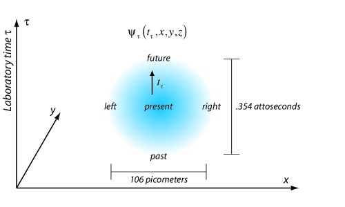
figure-images-bound-disp-0\hyper@anchorend

It takes about 150 attoseconds for an electron to circle the nucleus of an atom. An attosecond is 10-18 seconds long, or, expressed in another way, an attosecond is related to a second as a second is related to the age of the universe.

— Johan Mauritsson [924]

We now estimate the dispersion in quantum time of the wave functions.

We recall that the Coulomb potential is mediated by the exchange of virtual photons between electron and nucleus. These make it energetically favorable for oppositely charged particles to stay closer, subject to the restrictions of the Heisenberg uncertainty principle and the Pauli exclusion principle.

It is reasonable to suppose that if the paths of nucleus and electron get too far apart in time – or too close – the joint path will be disfavored for the same reasons.

By our principle of the maximum possible symmetry between time and space, our best order of magnitude estimate of the width of an atomic state in time is its width in space, divided by the speed of light. In natural units:

\Hy@raisedlink\hyper@anchorstartequationbounddispbounddisp9\hyper@anchorendσn¯22dr|ξn¯(r)|2r2similar-to\Hy@raisedlink\hyper@anchorstart𝑒𝑞𝑢𝑎𝑡𝑖𝑜𝑛𝑏𝑜𝑢𝑛𝑑𝑑𝑖𝑠𝑝𝑏𝑜𝑢𝑛𝑑𝑑𝑖𝑠𝑝9\hyper@anchorendsuperscriptsubscript𝜎¯𝑛22d𝑟superscriptsubscript𝜉¯𝑛𝑟2superscript𝑟2\Hy@raisedlink{\hyper@anchorstart{equation-bound-disp-bound-disp-9}\hyper@anchorend}\frac{{\sigma}_{\overline{n}}^{2}}{2}\sim{\displaystyle\int\text{d}\overrightarrow{r}{\left|{\xi}_{\overline{n}}\left(\overrightarrow{r}\right)\right|}^{2}{\overrightarrow{r}}^{2}} (4.159)

For an argon atom, as used in [734], the radius of the atom is 106 picometers. So our order of magnitude estimate of the width in time is less than an attosecond:

\Hy@raisedlink\hyper@anchorstartequationbounddispbounddisp8\hyper@anchorend1061012m3.00108m/s=.3541018s\Hy@raisedlink\hyper@anchorstart𝑒𝑞𝑢𝑎𝑡𝑖𝑜𝑛𝑏𝑜𝑢𝑛𝑑𝑑𝑖𝑠𝑝𝑏𝑜𝑢𝑛𝑑𝑑𝑖𝑠𝑝8\hyper@anchorend106superscript1012𝑚3.00superscript108𝑚𝑠.354superscript1018𝑠\Hy@raisedlink{\hyper@anchorstart{equation-bound-disp-bound-disp-8}\hyper@anchorend}\frac{106\cdot{10}^{-12}m}{3.00\cdot{10}^{8}m/s}=.354\cdot{10}^{-18}s (4.160)

This is exceedingly small 101010In practice we might want to work with Rydberg atoms, with very high principal quantum number, as these can be much wider..

As noted, to compute the dispersion from first principles we would have to calculate the bound states. To do this we would have to extend temporal quantization to the multi-particle case, then compute the ladder diagrams corresponding to virtual photon exchange between electron and nucleus. The poles in the resulting kernel give the bound state energies; the residues at the poles the wave functions.

However extending temporal quantization to the multi-particle case is a significant project in its own right, not part of this "testable chunk".

Chapter 5 Experimental Tests

\Hy@raisedlink\hyper@anchorstart

xt\hyper@anchorend

5.1 Overview

\Hy@raisedlink\hyper@anchorstart

xt-intro\hyper@anchorend

I will listen to any hypothesis but on one condition–that you show me a method by which it can be tested.

— August William Von Hoffman [751]

In the previous chapter we were looking at limits in which temporal quantization reduces to standard quantum theory. In this we are looking for differences, for ways to test for temporal quantization.

Our analysis is simplified by the absence of free parameters in temporal quantization; the properties of quantum time are forced by the requirement of manifest covariance. It is complicated by the fact we do not know what the initial wave function looks like.

In general we can force the issue by running the particle or beam through a chopper before making use of it in the experiment proper. If the chopper is open for a time $\Delta{\tau}_{chopper}$, and the particle has a roughly equal chance of getting through at any time, then it is reasonable to assume that the wave function has dispersion in time of order $\Delta{\tau}_{chopper}$:

\Hy@raisedlink\hyper@anchorstartequationxtintroxtinitial1\hyper@anchorendt2t2Δτchopper2similar-to\Hy@raisedlink\hyper@anchorstart𝑒𝑞𝑢𝑎𝑡𝑖𝑜𝑛𝑥𝑡𝑖𝑛𝑡𝑟𝑜𝑥𝑡𝑖𝑛𝑖𝑡𝑖𝑎𝑙1\hyper@anchorenddelimited-⟨⟩superscript𝑡2superscriptdelimited-⟨⟩𝑡2Δsuperscriptsubscript𝜏𝑐𝑜𝑝𝑝𝑒𝑟2\Hy@raisedlink{\hyper@anchorstart{equation-xt-intro-xt-initial-1}\hyper@anchorend}\langle{t}^{2}\rangle-{\langle t\rangle}^{2}\sim\Delta{\tau}_{chopper}^{2} (5.1)

If we think in terms of a classic experiment – beam aimed at target – then in addition to working with a particle with known or estimated dispersion in time, we will need to work with a target which in some way varies in time. Otherwise any effects are likely to be averaged away.

There are three obvious approaches. We can:

  1. 1.

    Start with an existing foundational experiment in quantum mechanics 111See the reviews of experimental tests of quantum mechanics in [715][462][105]., then interchange time and a space dimension. For instance, the double slit experiment becomes the double slit in time experiment if we replace the slits with choppers.

  2. 2.

    Run a particle with known dispersion in time through an electromagnetic field which is varying rapidly in time.

  3. 3.

    Take an experiment which implicitly takes a holistic view of time – the quantum eraser ([1030]), the Aharonov-Bohm experiment ([14]), tests of the Aharonov-Bergmann-Lebowitz ([13]) time-symmetric measurement – and re-examine from the perspective of quantum time.

We will look at examples of each of these approaches in turn, considering:

  1. 1.

    Slits in Time,

  2. 2.

    Time-varying Magnetic and Electric Fields,

  3. 3.

    And the Aharonov-Bohm Experiment.

As noted, we primarily interested in "proof-of-concept" here, so we will only look at the lowest nontrivial corrections resulting from quantum time. We will discuss various ways to make the treatments exact at the end of this chapter.

5.2 Slits in Time

\Hy@raisedlink\hyper@anchorstart

xt-gates\hyper@anchorend

5.2.1 Overview

\Hy@raisedlink\hyper@anchorstart

xt-gintro\hyper@anchorend

Here no one else can enter, since this gate was only for you. I now close it.

— K’s Gatekeeper [646]

At the narrow passage, there is no brother, no friend.

— Arab Proverb

Experiments

We will look at:

  1. 1.

    The Free Case,

  2. 2.

    The Single Slit Experiment,

  3. 3.

    The Double Slit Experiment,

  4. 4.

    And Lindner’s Attosecond Double Slit in Time  ([734]).

Approach

We take the particles as going left to right in the x  direction; the slits as choppers in the time direction. We start the particles off at x  position zero. The distance from the start to the gate is ${L}_{G}$, the distance from the start to the detector is ${L}_{D}$.

We model the particles as a set of rays in momentum space 222This is an example of the breakout of the initial wave function into Gaussian test functions proposed in Covariant Definition of Laboratory Time., each with an associated wave function in quantum time:

\Hy@raisedlink\hyper@anchorstartequationxtgintroxtgates3\hyper@anchorendψ(t,p)=χ(t,p)ξ^(p)\Hy@raisedlink\hyper@anchorstart𝑒𝑞𝑢𝑎𝑡𝑖𝑜𝑛𝑥𝑡𝑔𝑖𝑛𝑡𝑟𝑜𝑥𝑡𝑔𝑎𝑡𝑒𝑠3\hyper@anchorend𝜓𝑡𝑝𝜒𝑡𝑝^𝜉𝑝\Hy@raisedlink{\hyper@anchorstart{equation-xt-gintro-xt-gates-3}\hyper@anchorend}\psi\left(t,p\right)=\chi\left(t,p\right)\widehat{\xi}\left(p\right) (5.2)

To do the corresponding analysis for the standard quantum theory case we drop the wave function in time. Essentially we are using the momentum rays as carriers.

To simplify the analysis we assume the laboratory time and corresponding momentum are related in a deterministic way by 333Since p  and $\delta\tau$  are equivalent we can parameterize the space part/carrier ray with either.:

\Hy@raisedlink\hyper@anchorstartequationxtgintroxtgatesptr\hyper@anchorendp=mLτ\Hy@raisedlink\hyper@anchorstart𝑒𝑞𝑢𝑎𝑡𝑖𝑜𝑛𝑥𝑡𝑔𝑖𝑛𝑡𝑟𝑜𝑥𝑡𝑔𝑎𝑡𝑒𝑠𝑝𝑡𝑟\hyper@anchorend𝑝𝑚𝐿𝜏\Hy@raisedlink{\hyper@anchorstart{equation-xt-gintro-xt-gates-ptr}\hyper@anchorend}p=\frac{mL}{\tau} (5.3)

Where $\tau$  and L  are the laboratory time and the distance. We will frequently expand this around the averages, keeping only terms of first order:

\Hy@raisedlink\hyper@anchorstartequationxtgintroxtgatesfirst\hyper@anchorendp¯+δp=mLτ¯+δτδpp¯δττ¯,δττ¯δpp¯formulae-sequence\Hy@raisedlink\hyper@anchorstart𝑒𝑞𝑢𝑎𝑡𝑖𝑜𝑛𝑥𝑡𝑔𝑖𝑛𝑡𝑟𝑜𝑥𝑡𝑔𝑎𝑡𝑒𝑠𝑓𝑖𝑟𝑠𝑡\hyper@anchorend¯𝑝𝛿𝑝𝑚𝐿¯𝜏𝛿𝜏𝛿𝑝¯𝑝𝛿𝜏¯𝜏𝛿𝜏¯𝜏𝛿𝑝¯𝑝\Hy@raisedlink{\hyper@anchorstart{equation-xt-gintro-xt-gates-first}\hyper@anchorend}\overline{p}+\delta p=\frac{mL}{\overline{\tau}+\delta\tau}\rightarrow\delta p\approx-\overline{p}\frac{\delta\tau}{\overline{\tau}},\delta\tau\approx-\overline{\tau}\frac{\delta p}{\overline{p}} (5.4)

To further simplify we will work with Gaussian gates, rather than the more traditional square. This was suggested by Feynman and Hibbs ([403]). These are easier to work with and a better fit to Lindner’s Attosecond Double Slit in Time, discussed below. In principle, thanks to Morlet wavelet decomposition, they are fully general.

We work in the non-relativistic regime. We use the non-relativistic decomposition in Time/Momentum Representation. We assume $\gamma=\frac{E}{m}\approx 1$.

We will assume we are able to estimate the initial dispersion in time, and that this dispersion does not vary significantly as a function of the momentum.

5.2.2 Free Case

\Hy@raisedlink\hyper@anchorstart

xt-free\hyper@anchorend

Refer to caption
Figure 5.1: Free Case
\Hy@raisedlink
\hyper@anchorstart

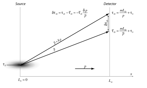
figure-images-xt-free-0\hyper@anchorend

We start by looking at the free case, to provide a reference point and to check the normalization.

Standard Quantum Theory

Per the analysis in Time/Momentum Representation  we take as the initial wave function in momentum:

\Hy@raisedlink\hyper@anchorstartequationxtfreextfreecarrier0\hyper@anchorendξ^S(p)=1πσ^124exp(δp22σ^12)\Hy@raisedlink\hyper@anchorstart𝑒𝑞𝑢𝑎𝑡𝑖𝑜𝑛𝑥𝑡𝑓𝑟𝑒𝑒𝑥𝑡𝑓𝑟𝑒𝑒𝑐𝑎𝑟𝑟𝑖𝑒𝑟0\hyper@anchorendsubscript^𝜉𝑆𝑝41𝜋superscriptsubscript^𝜎12exp𝛿superscript𝑝22superscriptsubscript^𝜎12\Hy@raisedlink{\hyper@anchorstart{equation-xt-free-xt-free-carrier-0}\hyper@anchorend}{\widehat{\xi}}_{S}\left(p\right)=\sqrt[4]{\frac{1}{\pi{\widehat{\sigma}}_{1}^{2}}}\mathrm{exp}\left(-\frac{\delta{p}^{2}}{2{\widehat{\sigma}}_{1}^{2}}\right) (5.5)

And get that the wave function at the detector is:

\Hy@raisedlink\hyper@anchorstartequationxtfreextfreecarrier2b\hyper@anchorendξ^D(p)=1πσ^124exp(δp22σ^12ip22mτDS)\Hy@raisedlink\hyper@anchorstart𝑒𝑞𝑢𝑎𝑡𝑖𝑜𝑛𝑥𝑡𝑓𝑟𝑒𝑒𝑥𝑡𝑓𝑟𝑒𝑒𝑐𝑎𝑟𝑟𝑖𝑒𝑟2𝑏\hyper@anchorendsubscript^𝜉𝐷𝑝41𝜋superscriptsubscript^𝜎12exp𝛿superscript𝑝22superscriptsubscript^𝜎12𝑖superscript𝑝22𝑚subscript𝜏𝐷𝑆\Hy@raisedlink{\hyper@anchorstart{equation-xt-free-xt-free-carrier-2b}\hyper@anchorend}{\widehat{\xi}}_{D}\left(p\right)=\sqrt[4]{\frac{1}{\pi{\widehat{\sigma}}_{1}^{2}}}\mathrm{exp}\left(-\frac{\delta{p}^{2}}{2{\widehat{\sigma}}_{1}^{2}}-i\frac{{p}^{2}}{2m}{\tau}_{DS}\right) (5.6)

With probability density:

\Hy@raisedlink\hyper@anchorstartequationxtfreextfreecarrier3\hyper@anchorendρ¯^D(δp)=1πσ^12exp(δp2σ^12)\Hy@raisedlink\hyper@anchorstart𝑒𝑞𝑢𝑎𝑡𝑖𝑜𝑛𝑥𝑡𝑓𝑟𝑒𝑒𝑥𝑡𝑓𝑟𝑒𝑒𝑐𝑎𝑟𝑟𝑖𝑒𝑟3\hyper@anchorendsubscript^¯𝜌𝐷𝛿𝑝1𝜋superscriptsubscript^𝜎12exp𝛿superscript𝑝2superscriptsubscript^𝜎12\Hy@raisedlink{\hyper@anchorstart{equation-xt-free-xt-free-carrier-3}\hyper@anchorend}{\widehat{\overline{\rho}}}_{D}\left(\delta p\right)=\sqrt{\frac{1}{\pi{\widehat{\sigma}}_{1}^{2}}}\mathrm{exp}\left(-\frac{\delta{p}^{2}}{{\widehat{\sigma}}_{1}^{2}}\right) (5.7)

Actual measurements are of clicks per unit time, not per unit momentum.

In going from momentum to laboratory time the probability density scales as the Jacobian:

\Hy@raisedlink\hyper@anchorstartequationxtfreextfreecarrier8\hyper@anchorenddpp¯τ¯Ddτρ¯^(δp)p¯τ¯Dρ¯^(p¯δτDτ¯D)=ρ¯(δτD)\Hy@raisedlink\hyper@anchorstart𝑒𝑞𝑢𝑎𝑡𝑖𝑜𝑛𝑥𝑡𝑓𝑟𝑒𝑒𝑥𝑡𝑓𝑟𝑒𝑒𝑐𝑎𝑟𝑟𝑖𝑒𝑟8\hyper@anchorendd𝑝¯𝑝subscript¯𝜏𝐷d𝜏^¯𝜌𝛿𝑝¯𝑝subscript¯𝜏𝐷^¯𝜌¯𝑝𝛿subscript𝜏𝐷subscript¯𝜏𝐷¯𝜌𝛿subscript𝜏𝐷\Hy@raisedlink{\hyper@anchorstart{equation-xt-free-xt-free-carrier-8}\hyper@anchorend}\text{d}p\rightarrow\frac{\overline{p}}{{\overline{\tau}}_{D}}\text{d}\tau\Rightarrow\widehat{\overline{\rho}}\left(\delta p\right)\rightarrow\frac{\overline{p}}{{\overline{\tau}}_{D}}\widehat{\overline{\rho}}\left(-\overline{p}\frac{\delta{\tau}_{D}}{{\overline{\tau}}_{D}}\right)=\overline{\rho}\left(\delta{\tau}_{D}\right) (5.8)

So the wave function scales as the square root of the Jacobian:

\Hy@raisedlink\hyper@anchorstartequationxtfreextfreecarrier9\hyper@anchorendξ^D(δpD)p¯τ¯DξD(δτD)\Hy@raisedlink\hyper@anchorstart𝑒𝑞𝑢𝑎𝑡𝑖𝑜𝑛𝑥𝑡𝑓𝑟𝑒𝑒𝑥𝑡𝑓𝑟𝑒𝑒𝑐𝑎𝑟𝑟𝑖𝑒𝑟9\hyper@anchorendsubscript^𝜉𝐷𝛿subscript𝑝𝐷¯𝑝subscript¯𝜏𝐷subscript𝜉𝐷𝛿subscript𝜏𝐷\Hy@raisedlink{\hyper@anchorstart{equation-xt-free-xt-free-carrier-9}\hyper@anchorend}{\widehat{\xi}}_{D}\left(\delta{p}_{D}\right)\rightarrow\sqrt{\frac{\overline{p}}{{\overline{\tau}}_{D}}}{\xi}_{D}\left(\delta{\tau}_{D}\right) (5.9)

The wave function as a function of $\delta{\tau}_{D}$  is then (dropping a term cubic in $\delta{\tau}_{D}$):

\Hy@raisedlink\hyper@anchorstartequationxtfreextfreecarrierc\hyper@anchorendξD(δτD)=1πσ¯D24exp(δτD22σ¯D2ip¯22mτ¯D+ip¯22mδτD+ip¯22mδτD2τ¯D)\Hy@raisedlink\hyper@anchorstart𝑒𝑞𝑢𝑎𝑡𝑖𝑜𝑛𝑥𝑡𝑓𝑟𝑒𝑒𝑥𝑡𝑓𝑟𝑒𝑒𝑐𝑎𝑟𝑟𝑖𝑒𝑟𝑐\hyper@anchorendsubscript𝜉𝐷𝛿subscript𝜏𝐷41𝜋superscriptsubscript¯𝜎𝐷2exp𝛿superscriptsubscript𝜏𝐷22superscriptsubscript¯𝜎𝐷2𝑖superscript¯𝑝22𝑚subscript¯𝜏𝐷𝑖superscript¯𝑝22𝑚𝛿subscript𝜏𝐷𝑖superscript¯𝑝22𝑚𝛿superscriptsubscript𝜏𝐷2subscript¯𝜏𝐷\Hy@raisedlink{\hyper@anchorstart{equation-xt-free-xt-free-carrier-c}\hyper@anchorend}{\xi}_{D}\left(\delta{\tau}_{D}\right)=\sqrt[4]{\frac{1}{\pi{\overline{\sigma}}_{D}^{2}}}\mathrm{exp}\left(-\frac{\delta{\tau}_{D}^{2}}{2{\overline{\sigma}}_{D}^{2}}-i\frac{{\overline{p}}^{2}}{2m}{\overline{\tau}}_{D}+i\frac{{\overline{p}}^{2}}{2m}\delta{\tau}_{D}+i\frac{{\overline{p}}^{2}}{2m}\frac{\delta{\tau}_{D}^{2}}{{\overline{\tau}}_{D}}\right) (5.10)

With the dispersion in laboratory time:

\Hy@raisedlink\hyper@anchorstartequationxtfreextfreecarrierf\hyper@anchorendσ¯D2=σ^12p¯2τ¯D2\Hy@raisedlink\hyper@anchorstart𝑒𝑞𝑢𝑎𝑡𝑖𝑜𝑛𝑥𝑡𝑓𝑟𝑒𝑒𝑥𝑡𝑓𝑟𝑒𝑒𝑐𝑎𝑟𝑟𝑖𝑒𝑟𝑓\hyper@anchorendsuperscriptsubscript¯𝜎𝐷2superscriptsubscript^𝜎12superscript¯𝑝2superscriptsubscript¯𝜏𝐷2\Hy@raisedlink{\hyper@anchorstart{equation-xt-free-xt-free-carrier-f}\hyper@anchorend}{\overline{\sigma}}_{D}^{2}=\frac{{\widehat{\sigma}}_{1}^{2}}{{\overline{p}}^{2}}{\overline{\tau}}_{D}^{2} (5.11)

This is the angular width of the beam, $\frac{{\widehat{\sigma}}_{1}}{\overline{p}}$, scaled by the laboratory time.

The probability density as a function of $\delta{\tau}_{D}$  is:

\Hy@raisedlink\hyper@anchorstartequationxtfreextfreecarriere\hyper@anchorendρ¯D(δτD)=1πσ¯D2exp(δτD2σ¯D2)\Hy@raisedlink\hyper@anchorstart𝑒𝑞𝑢𝑎𝑡𝑖𝑜𝑛𝑥𝑡𝑓𝑟𝑒𝑒𝑥𝑡𝑓𝑟𝑒𝑒𝑐𝑎𝑟𝑟𝑖𝑒𝑟𝑒\hyper@anchorendsubscript¯𝜌𝐷𝛿subscript𝜏𝐷1𝜋superscriptsubscript¯𝜎𝐷2exp𝛿superscriptsubscript𝜏𝐷2superscriptsubscript¯𝜎𝐷2\Hy@raisedlink{\hyper@anchorstart{equation-xt-free-xt-free-carrier-e}\hyper@anchorend}{\overline{\rho}}_{D}\left(\delta{\tau}_{D}\right)=\sqrt{\frac{1}{\pi{\overline{\sigma}}_{D}^{2}}}\mathrm{exp}\left(-\frac{\delta{\tau}_{D}^{2}}{{\overline{\sigma}}_{D}^{2}}\right) (5.12)

The normalization is already correct; no adjustment is required.

Temporal Quantization

We start at laboratory time ${\tau}_{\text{S}}$. We have the corresponding wave function in quantum time, non-relativistic, again from the analysis in Time/Momentum Representation:

\Hy@raisedlink\hyper@anchorstartequationxtfreextfree00\hyper@anchorendχS(tS,p)=1πσ024exp(iE¯ptS(tSt¯S)2σ02)\Hy@raisedlink\hyper@anchorstart𝑒𝑞𝑢𝑎𝑡𝑖𝑜𝑛𝑥𝑡𝑓𝑟𝑒𝑒𝑥𝑡𝑓𝑟𝑒𝑒00\hyper@anchorendsubscript𝜒𝑆subscript𝑡𝑆𝑝41𝜋superscriptsubscript𝜎02exp𝑖subscript¯𝐸𝑝subscript𝑡𝑆subscript𝑡𝑆subscript¯𝑡𝑆2superscriptsubscript𝜎02\Hy@raisedlink{\hyper@anchorstart{equation-xt-free-xt-free-00}\hyper@anchorend}{\chi}_{S}\left({t}_{S},p\right)=\sqrt[4]{\frac{1}{\pi{\sigma}_{0}^{2}}}\mathrm{exp}\left(-i{\overline{E}}_{p}{t}_{S}-\frac{\left({t}_{S}-{\overline{t}}_{S}\right)}{2{\sigma}_{0}^{2}}\right) (5.13)

The relative time at the start is defined as ${t}_{S}\equiv t-{\tau}_{S}$. We assume the average relative time at the start is zero: ${\overline{t}}_{S}=0$.

We assume that the initial energy is onshell:

\Hy@raisedlink\hyper@anchorstartequationxtfreextfree1\hyper@anchorendE¯pm2+p2m+p22m\Hy@raisedlink\hyper@anchorstart𝑒𝑞𝑢𝑎𝑡𝑖𝑜𝑛𝑥𝑡𝑓𝑟𝑒𝑒𝑥𝑡𝑓𝑟𝑒𝑒1\hyper@anchorendsubscript¯𝐸𝑝superscript𝑚2superscript𝑝2𝑚superscript𝑝22𝑚\Hy@raisedlink{\hyper@anchorstart{equation-xt-free-xt-free-1}\hyper@anchorend}{\overline{E}}_{p}\equiv\sqrt{{m}^{2}+{p}^{2}}\approx m+\frac{{p}^{2}}{2m} (5.14)

And therefore at the detector:

\Hy@raisedlink\hyper@anchorstartequationxtfreextfree0\hyper@anchorendχD(tD,p)=1πσ02fDS(0)4exp(iE¯ptD(tDt¯D)22σ02fDS(0)imτDS)\Hy@raisedlink\hyper@anchorstart𝑒𝑞𝑢𝑎𝑡𝑖𝑜𝑛𝑥𝑡𝑓𝑟𝑒𝑒𝑥𝑡𝑓𝑟𝑒𝑒0\hyper@anchorendsubscript𝜒𝐷subscript𝑡𝐷𝑝41𝜋superscriptsubscript𝜎02superscriptsubscript𝑓𝐷𝑆0exp𝑖subscript¯𝐸𝑝subscript𝑡𝐷superscriptsubscript𝑡𝐷subscript¯𝑡𝐷22superscriptsubscript𝜎02superscriptsubscript𝑓𝐷𝑆0𝑖𝑚subscript𝜏𝐷𝑆\Hy@raisedlink{\hyper@anchorstart{equation-xt-free-xt-free-0}\hyper@anchorend}{\chi}_{D}\left({t}_{D},p\right)=\sqrt[4]{\frac{1}{\pi{\sigma}_{0}^{2}{f}_{DS}^{\left(0\right)}}}\mathrm{exp}\left(-i{\overline{E}}_{p}{t}_{D}-\frac{{\left({t}_{D}-{\overline{t}}_{D}\right)}^{2}}{2{\sigma}_{0}^{2}{f}_{DS}^{\left(0\right)}}-im{\tau}_{DS}\right) (5.15)

With:

\Hy@raisedlink\hyper@anchorstartequationxtfreextfree2\hyper@anchorendt¯D=t¯S+(E¯pm1)τDS0\Hy@raisedlink\hyper@anchorstart𝑒𝑞𝑢𝑎𝑡𝑖𝑜𝑛𝑥𝑡𝑓𝑟𝑒𝑒𝑥𝑡𝑓𝑟𝑒𝑒2\hyper@anchorendsubscript¯𝑡𝐷subscript¯𝑡𝑆subscript¯𝐸𝑝𝑚1subscript𝜏𝐷𝑆0\Hy@raisedlink{\hyper@anchorstart{equation-xt-free-xt-free-2}\hyper@anchorend}{\overline{t}}_{D}={\overline{t}}_{S}+\left(\frac{{\overline{E}}_{p}}{m}-1\right){\tau}_{DS}\approx 0 (5.16)

Further we assume that the variation in starting time ${\tau}_{\text{S}}$  is small compared to the time to the detector ${\tau}_{\text{D}}$  so:

\Hy@raisedlink\hyper@anchorstartequationxtfreextfree3b\hyper@anchorendfDS(0)=1iτDSmσ021iτDmσ02\Hy@raisedlink\hyper@anchorstart𝑒𝑞𝑢𝑎𝑡𝑖𝑜𝑛𝑥𝑡𝑓𝑟𝑒𝑒𝑥𝑡𝑓𝑟𝑒𝑒3𝑏\hyper@anchorendsuperscriptsubscript𝑓𝐷𝑆01𝑖subscript𝜏𝐷𝑆𝑚superscriptsubscript𝜎021𝑖subscript𝜏𝐷𝑚superscriptsubscript𝜎02\Hy@raisedlink{\hyper@anchorstart{equation-xt-free-xt-free-3b}\hyper@anchorend}{f}_{DS}^{\left(0\right)}=1-i\frac{{\tau}_{DS}}{m{\sigma}_{0}^{2}}\approx 1-i\frac{{\tau}_{D}}{m{\sigma}_{0}^{2}} (5.17)

The wave function in time is then:

\Hy@raisedlink\hyper@anchorstartequationxtfreextfree5\hyper@anchorendχD(tD,p)=1πσ02fD(0)4exp(iE¯ptDtD22σ02fD(0)imτDS)\Hy@raisedlink\hyper@anchorstart𝑒𝑞𝑢𝑎𝑡𝑖𝑜𝑛𝑥𝑡𝑓𝑟𝑒𝑒𝑥𝑡𝑓𝑟𝑒𝑒5\hyper@anchorendsubscript𝜒𝐷subscript𝑡𝐷𝑝41𝜋superscriptsubscript𝜎02superscriptsubscript𝑓𝐷0exp𝑖subscript¯𝐸𝑝subscript𝑡𝐷superscriptsubscript𝑡𝐷22superscriptsubscript𝜎02superscriptsubscript𝑓𝐷0𝑖𝑚subscript𝜏𝐷𝑆\Hy@raisedlink{\hyper@anchorstart{equation-xt-free-xt-free-5}\hyper@anchorend}{\chi}_{D}\left({t}_{D},p\right)=\sqrt[4]{\frac{1}{\pi{\sigma}_{0}^{2}{f}_{D}^{\left(0\right)}}}\mathrm{exp}\left(-i{\overline{E}}_{p}{t}_{D}-\frac{{t}_{D}^{2}}{2{\sigma}_{0}^{2}{f}_{D}^{\left(0\right)}}-im{\tau}_{DS}\right) (5.18)

With the corresponding probability density in time for a specific ray p:

\Hy@raisedlink\hyper@anchorstartequationxtfreextfreetime8\hyper@anchorendρD(tD,p)=1πσD2exp(tD2σD2),σD2σ02|fD(0)|2=σ02(1+τ¯D2m2σ04)\Hy@raisedlink{\hyper@anchorstart{equation-xt-free-xt-free-time-8}\hyper@anchorend}{\stackrel{{\scriptstyle\frown}}{{\rho}}}_{D}\left({t}_{D},p\right)=\sqrt{\frac{1}{\pi{\stackrel{{\scriptstyle\frown}}{{\sigma}}}_{D}^{2}}}\mathrm{exp}\left(-\frac{{t}_{D}^{2}}{{\stackrel{{\scriptstyle\frown}}{{\sigma}}}_{D}^{2}}\right),{\stackrel{{\scriptstyle\frown}}{{\sigma}}}_{D}^{2}\equiv{\sigma}_{0}^{2}{\left|{f}_{D}^{\left(0\right)}\right|}^{2}={\sigma}_{0}^{2}\left(1+\frac{{\overline{\tau}}_{D}^{2}}{{m}^{2}{\sigma}_{0}^{4}}\right) (5.19)

The full wave function, in time and momentum, is:

\Hy@raisedlink\hyper@anchorstartequationxtfreextfree6\hyper@anchorendψD(tD,p)=1πσ02fD(0)4exp(iE¯ptDtD22σ02fD(0)imτDS)1πσ^124exp(δp22σ^12ip22mτDS)\Hy@raisedlink\hyper@anchorstart𝑒𝑞𝑢𝑎𝑡𝑖𝑜𝑛𝑥𝑡𝑓𝑟𝑒𝑒𝑥𝑡𝑓𝑟𝑒𝑒6\hyper@anchorendsubscript𝜓𝐷subscript𝑡𝐷𝑝41𝜋superscriptsubscript𝜎02superscriptsubscript𝑓𝐷0exp𝑖subscript¯𝐸𝑝subscript𝑡𝐷superscriptsubscript𝑡𝐷22superscriptsubscript𝜎02superscriptsubscript𝑓𝐷0𝑖𝑚subscript𝜏𝐷𝑆41𝜋superscriptsubscript^𝜎12exp𝛿superscript𝑝22superscriptsubscript^𝜎12𝑖superscript𝑝22𝑚subscript𝜏𝐷𝑆\Hy@raisedlink{\hyper@anchorstart{equation-xt-free-xt-free-6}\hyper@anchorend}{\psi}_{D}\left({t}_{D},p\right)=\sqrt[4]{\frac{1}{\pi{\sigma}_{0}^{2}{f}_{D}^{\left(0\right)}}}\mathrm{exp}\left(-i{\overline{E}}_{p}{t}_{D}-\frac{{t}_{D}^{2}}{2{\sigma}_{0}^{2}{f}_{D}^{\left(0\right)}}-im{\tau}_{DS}\right)\sqrt[4]{\frac{1}{\pi{\widehat{\sigma}}_{1}^{2}}}\mathrm{exp}\left(-\frac{\delta{p}^{2}}{2{\widehat{\sigma}}_{1}^{2}}-i\frac{{p}^{2}}{2m}{\tau}_{DS}\right) (5.20)

And the corresponding probability density is:

\Hy@raisedlink\hyper@anchorstartequationxtfreextfreetime9\hyper@anchorendρD(tD,δp)=ρD(tD,δp)ρ¯D(δp)\Hy@raisedlink{\hyper@anchorstart{equation-xt-free-xt-free-time-9}\hyper@anchorend}{\rho}_{D}\left({t}_{D},\delta p\right)={\stackrel{{\scriptstyle\frown}}{{\rho}}}_{D}\left({t}_{D},\delta p\right){\overline{\rho}}_{D}\left(\delta p\right) (5.21)

Each wave function in time is centered on a different p  and therefore a different time at the detector ${\tau}_{\text{D}}$. To combine the wave functions in time, we first expand the laboratory time as a function of the momentum p, keeping only the first order correction in $\delta p$:

\Hy@raisedlink\hyper@anchorstartequationxtfreextfreetimeb\hyper@anchorendtD=tτD=tτ¯DδτDtτ¯D+τ¯Dδpp¯\Hy@raisedlink\hyper@anchorstart𝑒𝑞𝑢𝑎𝑡𝑖𝑜𝑛𝑥𝑡𝑓𝑟𝑒𝑒𝑥𝑡𝑓𝑟𝑒𝑒𝑡𝑖𝑚𝑒𝑏\hyper@anchorendsubscript𝑡𝐷𝑡subscript𝜏𝐷𝑡subscript¯𝜏𝐷𝛿subscript𝜏𝐷𝑡subscript¯𝜏𝐷subscript¯𝜏𝐷𝛿𝑝¯𝑝\Hy@raisedlink{\hyper@anchorstart{equation-xt-free-xt-free-time-b}\hyper@anchorend}{t}_{D}=t-{\tau}_{D}=t-{\overline{\tau}}_{D}-\delta{\tau}_{D}\approx t-{\overline{\tau}}_{D}+{\overline{\tau}}_{D}\frac{\delta p}{\overline{p}}-\cdots (5.22)

We rewrite the probability density for the time part:

\Hy@raisedlink\hyper@anchorstartequationxtfreextfreetimec\hyper@anchorendρD(t,δp)=1πσD2exp((tτ¯D+τ¯Dδpp¯)2σD2)1πσ^12exp(δp2σ^12)\Hy@raisedlink\hyper@anchorstart𝑒𝑞𝑢𝑎𝑡𝑖𝑜𝑛𝑥𝑡𝑓𝑟𝑒𝑒𝑥𝑡𝑓𝑟𝑒𝑒𝑡𝑖𝑚𝑒𝑐\hyper@anchorendsubscript𝜌𝐷𝑡𝛿𝑝1superscriptsubscriptsuperscript𝜎𝐷2𝜋absentexpsuperscript𝑡subscript¯𝜏𝐷subscript¯𝜏𝐷𝛿𝑝¯𝑝2superscriptsubscriptsuperscript𝜎𝐷21𝜋superscriptsubscript^𝜎12exp𝛿superscript𝑝2superscriptsubscript^𝜎12\Hy@raisedlink{\hyper@anchorstart{equation-xt-free-xt-free-time-c}\hyper@anchorend}{\rho}_{D}\left(t,\delta p\right)=\sqrt{\frac{1}{\pi{\stackrel{{\scriptstyle\frown}}{{\sigma}}}_{D}^{2}}}\mathrm{exp}\left(-\frac{{\left(t-{\overline{\tau}}_{D}+{\overline{\tau}}_{D}\frac{\delta p}{\overline{p}}\right)}^{2}}{{\stackrel{{\scriptstyle\frown}}{{\sigma}}}_{D}^{2}}\right)\sqrt{\frac{1}{\pi{\widehat{\sigma}}_{1}^{2}}}\mathrm{exp}\left(-\frac{\delta{p}^{2}}{{\widehat{\sigma}}_{1}^{2}}\right) (5.23)
Probability Density as a Function of Time

To get the probability density as a function of time we integrate over the momentum p:

\Hy@raisedlink\hyper@anchorstartequationxtfreextfreetimef\hyper@anchorendρD(t)=dp1πσD2exp((tτ¯D+τ¯Dδpp¯)2σD2)1πσ^12exp(δp2σ^12)\Hy@raisedlink\hyper@anchorstart𝑒𝑞𝑢𝑎𝑡𝑖𝑜𝑛𝑥𝑡𝑓𝑟𝑒𝑒𝑥𝑡𝑓𝑟𝑒𝑒𝑡𝑖𝑚𝑒𝑓\hyper@anchorendsubscript𝜌𝐷𝑡d𝑝1superscriptsubscriptsuperscript𝜎𝐷2𝜋absentexpsuperscript𝑡subscript¯𝜏𝐷subscript¯𝜏𝐷𝛿𝑝¯𝑝2superscriptsubscriptsuperscript𝜎𝐷21𝜋superscriptsubscript^𝜎12exp𝛿superscript𝑝2superscriptsubscript^𝜎12\Hy@raisedlink{\hyper@anchorstart{equation-xt-free-xt-free-time-f}\hyper@anchorend}{\rho}_{D}\left(t\right)={\displaystyle\int\text{d}p\sqrt{\frac{1}{\pi{\stackrel{{\scriptstyle\frown}}{{\sigma}}}_{D}^{2}}}\mathrm{exp}\left(-\frac{{\left(t-{\overline{\tau}}_{D}+{\overline{\tau}}_{D}\frac{\delta p}{\overline{p}}\right)}^{2}}{{\stackrel{{\scriptstyle\frown}}{{\sigma}}}_{D}^{2}}\right)\sqrt{\frac{1}{\pi{\widehat{\sigma}}_{1}^{2}}}\mathrm{exp}\left(-\frac{\delta{p}^{2}}{{\widehat{\sigma}}_{1}^{2}}\right)} (5.24)

Which gives:

\Hy@raisedlink\hyper@anchorstartequationxtfreextfreetimeg\hyper@anchorendρD(t)=1πσD2exp((tτ¯D)2σD2)\Hy@raisedlink\hyper@anchorstart𝑒𝑞𝑢𝑎𝑡𝑖𝑜𝑛𝑥𝑡𝑓𝑟𝑒𝑒𝑥𝑡𝑓𝑟𝑒𝑒𝑡𝑖𝑚𝑒𝑔\hyper@anchorendsubscript𝜌𝐷𝑡1𝜋superscriptsubscript𝜎𝐷2expsuperscript𝑡subscript¯𝜏𝐷2superscriptsubscript𝜎𝐷2\Hy@raisedlink{\hyper@anchorstart{equation-xt-free-xt-free-time-g}\hyper@anchorend}{\rho}_{D}\left(t\right)=\frac{1}{\sqrt{\pi{\sigma}_{D}^{2}}}\mathrm{exp}\left(-\frac{{\left(t-{\overline{\tau}}_{D}\right)}^{2}}{{\sigma}_{D}^{2}}\right) (5.25)

Where the total dispersion in time breaks out cleanly into the sum of $t$  and p  parts:

\Hy@raisedlink\hyper@anchorstartequationxtfreextfreetimeh\hyper@anchorendσD2=σD2+σ¯D2\Hy@raisedlink{\hyper@anchorstart{equation-xt-free-xt-free-time-h}\hyper@anchorend}{\sigma}_{D}^{2}={\stackrel{{\scriptstyle\frown}}{{\sigma}}}_{D}^{2}+{\overline{\sigma}}_{D}^{2} (5.26)

Or:

\Hy@raisedlink\hyper@anchorstartequationxtfreextfreetimei\hyper@anchorendσD2=σ02+(1m2σ02+σ^12p¯2)τ¯D2>σ¯D2=σ^12p¯2τ¯D2\Hy@raisedlink\hyper@anchorstart𝑒𝑞𝑢𝑎𝑡𝑖𝑜𝑛𝑥𝑡𝑓𝑟𝑒𝑒𝑥𝑡𝑓𝑟𝑒𝑒𝑡𝑖𝑚𝑒𝑖\hyper@anchorendsuperscriptsubscript𝜎𝐷2superscriptsubscript𝜎021superscript𝑚2superscriptsubscript𝜎02superscriptsubscript^𝜎12superscript¯𝑝2superscriptsubscript¯𝜏𝐷2superscriptsubscript¯𝜎𝐷2superscriptsubscript^𝜎12superscript¯𝑝2superscriptsubscript¯𝜏𝐷2\Hy@raisedlink{\hyper@anchorstart{equation-xt-free-xt-free-time-i}\hyper@anchorend}{\sigma}_{D}^{2}={\sigma}_{0}^{2}+\left(\frac{1}{{m}^{2}{\sigma}_{0}^{2}}+\frac{{\widehat{\sigma}}_{1}^{2}}{{\overline{p}}^{2}}\right){\overline{\tau}}_{D}^{2}>{\overline{\sigma}}_{D}^{2}=\frac{{\widehat{\sigma}}_{1}^{2}}{{\overline{p}}^{2}}{\overline{\tau}}_{D}^{2} (5.27)

By comparison to the standard quantum theory’s dispersion in laboratory time, the dispersion in laboratory time in temporal quantization:

  1. 1.

    Starts off non-zero (from the initial dispersion of the wave function in time),

  2. 2.

    Grows more rapidly with laboratory time (as one would expect from a theory of fuzzy time).

5.2.3 Single Slit Experiment

\Hy@raisedlink\hyper@anchorstart

xt-single\hyper@anchorend

Refer to caption
Figure 5.2: Single Slit With Gaussian Gate
\Hy@raisedlink
\hyper@anchorstart

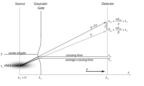
figure-images-xt-single-1\hyper@anchorend

With the results for the free particle in hand, we look at what happens when the free Gaussian test function encounters a gate.

The single gate experiment is:

  1. 1.

    Interesting in its own right,

  2. 2.

    A fundamental building block in the analysis of the double slit experiment,

  3. 3.

    And a useful preparatory step in most tests of quantum time.

5.2.3.1 Gaussian Gates
\Hy@raisedlink\hyper@anchorstart

xt-sgate\hyper@anchorend

In Laboratory Time

We work with Gaussian gates (see [403]). We take the gate as centered on time T  with width ${\Sigma}_{G}$. As a function of laboratory time ${\tau}_{\text{G}}$  the gate is given by:

\Hy@raisedlink\hyper@anchorstartequationxtsgatextsgate00\hyper@anchorendG¯G(T)=exp((τGT)22ΣG2)=exp(TG22ΣG2)\Hy@raisedlink\hyper@anchorstart𝑒𝑞𝑢𝑎𝑡𝑖𝑜𝑛𝑥𝑡𝑠𝑔𝑎𝑡𝑒𝑥𝑡𝑠𝑔𝑎𝑡𝑒00\hyper@anchorendsuperscriptsubscript¯𝐺𝐺𝑇expsuperscriptsubscript𝜏𝐺𝑇22superscriptsubscriptΣ𝐺2expsuperscriptsubscript𝑇𝐺22superscriptsubscriptΣ𝐺2\Hy@raisedlink{\hyper@anchorstart{equation-xt-sgate-xt-sgate-00}\hyper@anchorend}{\overline{G}}_{G}^{\left(T\right)}=\mathrm{exp}\left(-\frac{{\left({\tau}_{G}-T\right)}^{2}}{2{\Sigma}_{G}^{2}}\right)=\mathrm{exp}\left(-\frac{{T}_{G}^{2}}{2{\Sigma}_{G}^{2}}\right) (5.28)

Given p, the time of arrival at the gate is given by ${\tau}_{\text{G}}$:

\Hy@raisedlink\hyper@anchorstartequationxtsgatextsgate0\hyper@anchorendτG=mLGp+τS,τ¯G=mLGp¯+τSformulae-sequence\Hy@raisedlink\hyper@anchorstart𝑒𝑞𝑢𝑎𝑡𝑖𝑜𝑛𝑥𝑡𝑠𝑔𝑎𝑡𝑒𝑥𝑡𝑠𝑔𝑎𝑡𝑒0\hyper@anchorendsubscript𝜏𝐺𝑚subscript𝐿𝐺𝑝subscript𝜏𝑆subscript¯𝜏𝐺𝑚subscript𝐿𝐺¯𝑝subscript𝜏𝑆\Hy@raisedlink{\hyper@anchorstart{equation-xt-sgate-xt-sgate-0}\hyper@anchorend}{\tau}_{G}=\frac{m{L}_{G}}{p}+{\tau}_{S},{\overline{\tau}}_{G}=\frac{m{L}_{G}}{\overline{p}}+{\tau}_{S} (5.29)

We can write the T  associated with the gate in relative time:

\Hy@raisedlink\hyper@anchorstartequationxtsgatextsgate3\hyper@anchorendTGTτG,TG¯Tτ¯Gformulae-sequence\Hy@raisedlink\hyper@anchorstart𝑒𝑞𝑢𝑎𝑡𝑖𝑜𝑛𝑥𝑡𝑠𝑔𝑎𝑡𝑒𝑥𝑡𝑠𝑔𝑎𝑡𝑒3\hyper@anchorendsubscript𝑇𝐺𝑇subscript𝜏𝐺subscript𝑇¯𝐺𝑇subscript¯𝜏𝐺\Hy@raisedlink{\hyper@anchorstart{equation-xt-sgate-xt-sgate-3}\hyper@anchorend}{T}_{G}\equiv T-{\tau}_{G},{T}_{\overline{G}}\equiv T-{\overline{\tau}}_{G} (5.30)

${T}_{\overline{G}}=0$  means the beam is dead center on the gate.

In Momentum Space

To solve for the single slit case in standard quantum theory we will need the gate as a function of the momentum p. To get this, we expand ${T}_{G}$  in terms of the momentum:

\Hy@raisedlink\hyper@anchorstartequationxtsgatextsgate1\hyper@anchorendTG=TG¯+τ¯Gδpp¯\Hy@raisedlink\hyper@anchorstart𝑒𝑞𝑢𝑎𝑡𝑖𝑜𝑛𝑥𝑡𝑠𝑔𝑎𝑡𝑒𝑥𝑡𝑠𝑔𝑎𝑡𝑒1\hyper@anchorendsubscript𝑇𝐺subscript𝑇¯𝐺subscript¯𝜏𝐺𝛿𝑝¯𝑝\Hy@raisedlink{\hyper@anchorstart{equation-xt-sgate-xt-sgate-1}\hyper@anchorend}{T}_{G}={T}_{\overline{G}}+{\overline{\tau}}_{G}\frac{\delta p}{\overline{p}} (5.31)

We use this to rewrite the gate function in momentum space:

\Hy@raisedlink\hyper@anchorstartequationxtsgatextsgate7\hyper@anchorendG¯^(P)(δp)=exp((δpP)22Σ^G2)\Hy@raisedlink\hyper@anchorstart𝑒𝑞𝑢𝑎𝑡𝑖𝑜𝑛𝑥𝑡𝑠𝑔𝑎𝑡𝑒𝑥𝑡𝑠𝑔𝑎𝑡𝑒7\hyper@anchorendsuperscript^¯𝐺𝑃𝛿𝑝expsuperscript𝛿𝑝𝑃22superscriptsubscript^Σ𝐺2\Hy@raisedlink{\hyper@anchorstart{equation-xt-sgate-xt-sgate-7}\hyper@anchorend}{\widehat{\overline{G}}}^{\left(P\right)}\left(\delta p\right)=\mathrm{exp}\left(-\frac{{\left(\delta p-P\right)}^{2}}{2{\widehat{\Sigma}}_{G}^{2}}\right) (5.32)

With the "effective momentum" of the gate:

\Hy@raisedlink\hyper@anchorstartequationxtsgatextsgate9\hyper@anchorendPTG¯τ¯Gp¯\Hy@raisedlink\hyper@anchorstart𝑒𝑞𝑢𝑎𝑡𝑖𝑜𝑛𝑥𝑡𝑠𝑔𝑎𝑡𝑒𝑥𝑡𝑠𝑔𝑎𝑡𝑒9\hyper@anchorend𝑃subscript𝑇¯𝐺subscript¯𝜏𝐺¯𝑝\Hy@raisedlink{\hyper@anchorstart{equation-xt-sgate-xt-sgate-9}\hyper@anchorend}P\equiv-\frac{{T}_{\overline{G}}}{{\overline{\tau}}_{G}}\overline{p} (5.33)

And the dispersion of the gate in momentum space:

\Hy@raisedlink\hyper@anchorstartequationxtsgatextsgate8\hyper@anchorendΣ^G2ΣG2τ¯G2p¯2\Hy@raisedlink\hyper@anchorstart𝑒𝑞𝑢𝑎𝑡𝑖𝑜𝑛𝑥𝑡𝑠𝑔𝑎𝑡𝑒𝑥𝑡𝑠𝑔𝑎𝑡𝑒8\hyper@anchorendsuperscriptsubscript^Σ𝐺2superscriptsubscriptΣ𝐺2superscriptsubscript¯𝜏𝐺2superscript¯𝑝2\Hy@raisedlink{\hyper@anchorstart{equation-xt-sgate-xt-sgate-8}\hyper@anchorend}{\widehat{\Sigma}}_{G}^{2}\equiv\frac{{\Sigma}_{G}^{2}}{{\overline{\tau}}_{G}^{2}}{\overline{p}}^{2} (5.34)
In Quantum Time

In block time the gate is:

\Hy@raisedlink\hyper@anchorstartequationxtsgatextsgatee\hyper@anchorendG(T)(t)=exp((tT)22ΣG2)\Hy@raisedlink\hyper@anchorstart𝑒𝑞𝑢𝑎𝑡𝑖𝑜𝑛𝑥𝑡𝑠𝑔𝑎𝑡𝑒𝑥𝑡𝑠𝑔𝑎𝑡𝑒𝑒\hyper@anchorendsuperscript𝐺𝑇𝑡expsuperscript𝑡𝑇22superscriptsubscriptΣ𝐺2\Hy@raisedlink{\hyper@anchorstart{equation-xt-sgate-xt-sgate-e}\hyper@anchorend}{G}^{\left(T\right)}\left(t\right)=\mathrm{exp}\left(-\frac{{\left(t-T\right)}^{2}}{2{\Sigma}_{G}^{2}}\right) (5.35)

In relative time the gate is:

\Hy@raisedlink\hyper@anchorstartequationxtsgatextsgatef\hyper@anchorendG(TG)(tG)=exp((tGTG)22ΣG2)\Hy@raisedlink\hyper@anchorstart𝑒𝑞𝑢𝑎𝑡𝑖𝑜𝑛𝑥𝑡𝑠𝑔𝑎𝑡𝑒𝑥𝑡𝑠𝑔𝑎𝑡𝑒𝑓\hyper@anchorendsuperscript𝐺subscript𝑇𝐺subscript𝑡𝐺expsuperscriptsubscript𝑡𝐺subscript𝑇𝐺22superscriptsubscriptΣ𝐺2\Hy@raisedlink{\hyper@anchorstart{equation-xt-sgate-xt-sgate-f}\hyper@anchorend}{G}^{\left({T}_{G}\right)}\left({t}_{G}\right)=\mathrm{exp}\left(-\frac{{\left({t}_{G}-{T}_{G}\right)}^{2}}{2{\Sigma}_{G}^{2}}\right) (5.36)
5.2.3.2 Standard Quantum Theory
\Hy@raisedlink\hyper@anchorstart

xt-ssqt\hyper@anchorend

We first solve for the probability distribution in time at the detector in standard quantum theory. To get the wave function at the detector we use a kernel to get the wave function up to the detector, multiply by the gate function, then apply another kernel to get from gate to detector.

In Momentum Space

The wave function at the detector in momentum space is given by:

\Hy@raisedlink\hyper@anchorstartequationxtssqtxtssqtderiv0\hyper@anchorendξ^D(pD)=dpGK¯^DG(pD;pG)G¯^(P)(pG)dpSK¯^G(pG;pS)ξ^S(pS)\Hy@raisedlink\hyper@anchorstart𝑒𝑞𝑢𝑎𝑡𝑖𝑜𝑛𝑥𝑡𝑠𝑠𝑞𝑡𝑥𝑡𝑠𝑠𝑞𝑡𝑑𝑒𝑟𝑖𝑣0\hyper@anchorendsubscript^𝜉𝐷subscript𝑝𝐷dsubscript𝑝𝐺subscript^¯𝐾𝐷𝐺subscript𝑝𝐷subscript𝑝𝐺superscript^¯𝐺𝑃subscript𝑝𝐺dsubscript𝑝𝑆subscript^¯𝐾𝐺subscript𝑝𝐺subscript𝑝𝑆subscript^𝜉𝑆subscript𝑝𝑆\Hy@raisedlink{\hyper@anchorstart{equation-xt-ssqt-xt-ssqt-deriv-0}\hyper@anchorend}{\widehat{\xi}}_{D}\left({p}_{D}\right)={\displaystyle\int\text{d}{p}_{G}{\widehat{\overline{K}}}_{DG}\left({p}_{D};{p}_{G}\right){\widehat{\overline{G}}}^{\left(P\right)}\left({p}_{G}\right){\displaystyle\int\text{d}{p}_{S}{\widehat{\overline{K}}}_{G}\left({p}_{G};{p}_{S}\right){\widehat{\xi}}_{S}\left({p}_{S}\right)}} (5.37)

The kernels are just $\delta$  functions with a bit of phase, so the integrals are trivial:

\Hy@raisedlink\hyper@anchorstartequationxtssqtxtssqtderiv3\hyper@anchorendξ^D(δp)=1πσ^124exp(P22Σ^G2+PΣ^G2δpδp22Σ^G2δp22σ^12)exp(ip22mτDS)\Hy@raisedlink\hyper@anchorstart𝑒𝑞𝑢𝑎𝑡𝑖𝑜𝑛𝑥𝑡𝑠𝑠𝑞𝑡𝑥𝑡𝑠𝑠𝑞𝑡𝑑𝑒𝑟𝑖𝑣3\hyper@anchorendsubscript^𝜉𝐷𝛿𝑝41𝜋superscriptsubscript^𝜎12expsuperscript𝑃22superscriptsubscript^Σ𝐺2𝑃superscriptsubscript^Σ𝐺2𝛿𝑝𝛿superscript𝑝22superscriptsubscript^Σ𝐺2𝛿superscript𝑝22superscriptsubscript^𝜎12exp𝑖superscript𝑝22𝑚subscript𝜏𝐷𝑆\Hy@raisedlink{\hyper@anchorstart{equation-xt-ssqt-xt-ssqt-deriv-3}\hyper@anchorend}{\widehat{\xi}}_{D}\left(\delta p\right)=\sqrt[4]{\frac{1}{\pi{\widehat{\sigma}}_{1}^{2}}}\mathrm{exp}\left(-\frac{{P}^{2}}{2{\widehat{\Sigma}}_{G}^{2}}+\frac{P}{{\widehat{\Sigma}}_{G}^{2}}\delta p-\frac{\delta{p}^{2}}{2{\widehat{\Sigma}}_{G}^{2}}-\frac{\delta{p}^{2}}{2{\widehat{\sigma}}_{1}^{2}}\right)\mathrm{exp}\left(-i\frac{{p}^{2}}{2m}{\tau}_{DS}\right) (5.38)

We rewrite as a Gaussian test function times a normalization factor 444Essentially we are completing the square.:

\Hy@raisedlink\hyper@anchorstartequationxtssqtxtssqtderiv4\hyper@anchorendξ^D(δp)=N¯^(sqt)1πσ¯^G(sqt)24exp((δpδp(sqt))22σ¯^G(sqt)2ip22mτDS)\Hy@raisedlink\hyper@anchorstart𝑒𝑞𝑢𝑎𝑡𝑖𝑜𝑛𝑥𝑡𝑠𝑠𝑞𝑡𝑥𝑡𝑠𝑠𝑞𝑡𝑑𝑒𝑟𝑖𝑣4\hyper@anchorendsubscript^𝜉𝐷𝛿𝑝superscript^¯𝑁𝑠𝑞𝑡41𝜋superscriptsubscript^¯𝜎𝐺𝑠𝑞𝑡2expsuperscript𝛿𝑝𝛿superscript𝑝𝑠𝑞𝑡22superscriptsubscript^¯𝜎𝐺𝑠𝑞𝑡2𝑖superscript𝑝22𝑚subscript𝜏𝐷𝑆\Hy@raisedlink{\hyper@anchorstart{equation-xt-ssqt-xt-ssqt-deriv-4}\hyper@anchorend}{\widehat{\xi}}_{D}\left(\delta p\right)={\widehat{\overline{N}}}^{\left(sqt\right)}\sqrt[4]{\frac{1}{\pi{\widehat{\overline{\sigma}}}_{G}^{\left(sqt\right)2}}}\mathrm{exp}\left(-\frac{{\left(\delta p-\delta{p}^{\left(sqt\right)}\right)}^{2}}{2{\widehat{\overline{\sigma}}}_{G}^{\left(sqt\right)2}}-i\frac{{p}^{2}}{2m}{\tau}_{DS}\right) (5.39)

With dispersion, offset, and normalization:

\Hy@raisedlink\hyper@anchorstartequationxtssqtxtssqtderiv5\hyper@anchorendσ¯^G(sqt)2Σ^G2σ^12Σ^G2+σ^12\Hy@raisedlink\hyper@anchorstart𝑒𝑞𝑢𝑎𝑡𝑖𝑜𝑛𝑥𝑡𝑠𝑠𝑞𝑡𝑥𝑡𝑠𝑠𝑞𝑡𝑑𝑒𝑟𝑖𝑣5\hyper@anchorendsuperscriptsubscript^¯𝜎𝐺𝑠𝑞𝑡2superscriptsubscript^Σ𝐺2superscriptsubscript^𝜎12superscriptsubscript^Σ𝐺2superscriptsubscript^𝜎12\Hy@raisedlink{\hyper@anchorstart{equation-xt-ssqt-xt-ssqt-deriv-5}\hyper@anchorend}{\widehat{\overline{\sigma}}}_{G}^{\left(sqt\right)2}\equiv\frac{{\widehat{\Sigma}}_{G}^{2}{\widehat{\sigma}}_{1}^{2}}{{\widehat{\Sigma}}_{G}^{2}+{\widehat{\sigma}}_{1}^{2}} (5.40)
\Hy@raisedlink\hyper@anchorstartequationxtssqtxtssqtderiv6\hyper@anchorendδp(sqt)PΣ^G2σ¯^G(sqt)2\Hy@raisedlink\hyper@anchorstart𝑒𝑞𝑢𝑎𝑡𝑖𝑜𝑛𝑥𝑡𝑠𝑠𝑞𝑡𝑥𝑡𝑠𝑠𝑞𝑡𝑑𝑒𝑟𝑖𝑣6\hyper@anchorend𝛿superscript𝑝𝑠𝑞𝑡𝑃superscriptsubscript^Σ𝐺2superscriptsubscript^¯𝜎𝐺𝑠𝑞𝑡2\Hy@raisedlink{\hyper@anchorstart{equation-xt-ssqt-xt-ssqt-deriv-6}\hyper@anchorend}\delta{p}^{\left(sqt\right)}\equiv\frac{P}{{\widehat{\Sigma}}_{G}^{2}}{\widehat{\overline{\sigma}}}_{G}^{\left(sqt\right)2} (5.41)
\Hy@raisedlink\hyper@anchorstartequationxtssqtxtssqtderiv7\hyper@anchorendN¯^(sqt)σ¯^G(sqt)2σ^124exp(P22Σ^G2+δp(sqt)22σ¯^G(sqt)2)=Σ^G2Σ^G2+σ^124exp(12P2Σ^G2+σ^12)\Hy@raisedlink\hyper@anchorstart𝑒𝑞𝑢𝑎𝑡𝑖𝑜𝑛𝑥𝑡𝑠𝑠𝑞𝑡𝑥𝑡𝑠𝑠𝑞𝑡𝑑𝑒𝑟𝑖𝑣7\hyper@anchorendsuperscript^¯𝑁𝑠𝑞𝑡4superscriptsubscript^¯𝜎𝐺𝑠𝑞𝑡2superscriptsubscript^𝜎12expsuperscript𝑃22superscriptsubscript^Σ𝐺2𝛿superscript𝑝𝑠𝑞𝑡22superscriptsubscript^¯𝜎𝐺𝑠𝑞𝑡24superscriptsubscript^Σ𝐺2superscriptsubscript^Σ𝐺2superscriptsubscript^𝜎12exp12superscript𝑃2superscriptsubscript^Σ𝐺2superscriptsubscript^𝜎12\Hy@raisedlink{\hyper@anchorstart{equation-xt-ssqt-xt-ssqt-deriv-7}\hyper@anchorend}{\widehat{\overline{N}}}^{\left(sqt\right)}\equiv\sqrt[4]{\frac{{\widehat{\overline{\sigma}}}_{G}^{\left(sqt\right)2}}{{\widehat{\sigma}}_{1}^{2}}}\mathrm{exp}\left(-\frac{{P}^{2}}{2{\widehat{\Sigma}}_{G}^{2}}+\frac{\delta{p}^{\left(sqt\right)2}}{2{\widehat{\overline{\sigma}}}_{G}^{\left(sqt\right)2}}\right)=\sqrt[4]{\frac{{\widehat{\Sigma}}_{G}^{2}}{{\widehat{\Sigma}}_{G}^{2}+{\widehat{\sigma}}_{1}^{2}}}\mathrm{exp}\left(-\frac{1}{2}\frac{{P}^{2}}{{\widehat{\Sigma}}_{G}^{2}+{\widehat{\sigma}}_{1}^{2}}\right) (5.42)

And probability density:

\Hy@raisedlink\hyper@anchorstartequationxtssqtxtssqtderiv8\hyper@anchorendρ¯^D(δp)=N¯(sqt)21πσ¯^G(sqt)2exp((δpδp(sqt))2σ¯^G(sqt)2)\Hy@raisedlink\hyper@anchorstart𝑒𝑞𝑢𝑎𝑡𝑖𝑜𝑛𝑥𝑡𝑠𝑠𝑞𝑡𝑥𝑡𝑠𝑠𝑞𝑡𝑑𝑒𝑟𝑖𝑣8\hyper@anchorendsubscript^¯𝜌𝐷𝛿𝑝superscript¯𝑁𝑠𝑞𝑡21𝜋superscriptsubscript^¯𝜎𝐺𝑠𝑞𝑡2expsuperscript𝛿𝑝𝛿superscript𝑝𝑠𝑞𝑡2superscriptsubscript^¯𝜎𝐺𝑠𝑞𝑡2\Hy@raisedlink{\hyper@anchorstart{equation-xt-ssqt-xt-ssqt-deriv-8}\hyper@anchorend}{\widehat{\overline{\rho}}}_{D}\left(\delta p\right)={\overline{N}}^{\left(sqt\right)2}\sqrt{\frac{1}{\pi{\widehat{\overline{\sigma}}}_{G}^{\left(sqt\right)2}}}\mathrm{exp}\left(-\frac{{\left(\delta p-\delta{p}^{\left(sqt\right)}\right)}^{2}}{{\widehat{\overline{\sigma}}}_{G}^{\left(sqt\right)2}}\right) (5.43)
In Laboratory Time

We change coordinates from $\delta p$  to $\delta{\tau}_{D}$  using $\delta p\approx-\overline{p}\frac{\delta\tau}{\overline{\tau}}$:

\Hy@raisedlink\hyper@anchorstartequationxtssqtxtsingletau2\hyper@anchorendξD(δτD)=N¯(sqt)1πσ¯D(sqt)24exp((δτDδτD(sqt))22σ¯D(sqt)2)exp(ip¯22mτ¯D+ip¯22mδτD+ip¯22mδτD2τ¯D)\Hy@raisedlink\hyper@anchorstart𝑒𝑞𝑢𝑎𝑡𝑖𝑜𝑛𝑥𝑡𝑠𝑠𝑞𝑡𝑥𝑡𝑠𝑖𝑛𝑔𝑙𝑒𝑡𝑎𝑢2\hyper@anchorendsubscript𝜉𝐷𝛿subscript𝜏𝐷superscript¯𝑁𝑠𝑞𝑡41𝜋superscriptsubscript¯𝜎𝐷𝑠𝑞𝑡2expsuperscript𝛿subscript𝜏𝐷𝛿superscriptsubscript𝜏𝐷𝑠𝑞𝑡22superscriptsubscript¯𝜎𝐷𝑠𝑞𝑡2exp𝑖superscript¯𝑝22𝑚subscript¯𝜏𝐷𝑖superscript¯𝑝22𝑚𝛿subscript𝜏𝐷𝑖superscript¯𝑝22𝑚𝛿superscriptsubscript𝜏𝐷2subscript¯𝜏𝐷\Hy@raisedlink{\hyper@anchorstart{equation-xt-ssqt-xt-single-tau-2}\hyper@anchorend}{\xi}_{D}\left(\delta{\tau}_{D}\right)={\overline{N}}^{\left(sqt\right)}\sqrt[4]{\frac{1}{\pi{\overline{\sigma}}_{D}^{\left(sqt\right)2}}}\mathrm{exp}\left(-\frac{{\left(\delta{\tau}_{D}-\delta{\tau}_{D}^{\left(sqt\right)}\right)}^{2}}{2{\overline{\sigma}}_{D}^{\left(sqt\right)2}}\right)\mathrm{exp}\left(-i\frac{{\overline{p}}^{2}}{2m}{\overline{\tau}}_{D}+i\frac{{\overline{p}}^{2}}{2m}\delta{\tau}_{D}+i\frac{{\overline{p}}^{2}}{2m}\frac{\delta{\tau}_{D}^{2}}{{\overline{\tau}}_{D}}\right) (5.44)

With dispersion, offset, and normalization:

\Hy@raisedlink\hyper@anchorstartequationxtssqtxtsingletau3\hyper@anchorendσ¯D(sqt)2=ΣG2σ¯G2ΣG2+σ¯G2τ¯D2τ¯G2,σ¯G2=σ^12p¯2τ¯G2formulae-sequence\Hy@raisedlink\hyper@anchorstart𝑒𝑞𝑢𝑎𝑡𝑖𝑜𝑛𝑥𝑡𝑠𝑠𝑞𝑡𝑥𝑡𝑠𝑖𝑛𝑔𝑙𝑒𝑡𝑎𝑢3\hyper@anchorendsuperscriptsubscript¯𝜎𝐷𝑠𝑞𝑡2superscriptsubscriptΣ𝐺2superscriptsubscript¯𝜎𝐺2superscriptsubscriptΣ𝐺2superscriptsubscript¯𝜎𝐺2superscriptsubscript¯𝜏𝐷2superscriptsubscript¯𝜏𝐺2superscriptsubscript¯𝜎𝐺2superscriptsubscript^𝜎12superscript¯𝑝2superscriptsubscript¯𝜏𝐺2\Hy@raisedlink{\hyper@anchorstart{equation-xt-ssqt-xt-single-tau-3}\hyper@anchorend}{\overline{\sigma}}_{D}^{\left(sqt\right)2}=\frac{{\Sigma}_{G}^{2}{\overline{\sigma}}_{G}^{2}}{{\Sigma}_{G}^{2}+{\overline{\sigma}}_{G}^{2}}\frac{{\overline{\tau}}_{D}^{2}}{{\overline{\tau}}_{G}^{2}},{\overline{\sigma}}_{G}^{2}=\frac{{\widehat{\sigma}}_{1}^{2}}{{\overline{p}}^{2}}{\overline{\tau}}_{G}^{2} (5.45)
\Hy@raisedlink\hyper@anchorstartequationxtssqtxtsingletau4\hyper@anchorendδτD(sqt)=σ¯G2ΣG2+σ¯G2TG¯τ¯Gτ¯D\Hy@raisedlink\hyper@anchorstart𝑒𝑞𝑢𝑎𝑡𝑖𝑜𝑛𝑥𝑡𝑠𝑠𝑞𝑡𝑥𝑡𝑠𝑖𝑛𝑔𝑙𝑒𝑡𝑎𝑢4\hyper@anchorend𝛿superscriptsubscript𝜏𝐷𝑠𝑞𝑡superscriptsubscript¯𝜎𝐺2superscriptsubscriptΣ𝐺2superscriptsubscript¯𝜎𝐺2subscript𝑇¯𝐺subscript¯𝜏𝐺subscript¯𝜏𝐷\Hy@raisedlink{\hyper@anchorstart{equation-xt-ssqt-xt-single-tau-4}\hyper@anchorend}\delta{\tau}_{D}^{\left(sqt\right)}=-\frac{{\overline{\sigma}}_{G}^{2}}{{\Sigma}_{G}^{2}+{\overline{\sigma}}_{G}^{2}}\frac{{T}_{\overline{G}}}{{\overline{\tau}}_{G}}{\overline{\tau}}_{D} (5.46)
\Hy@raisedlink\hyper@anchorstartequationxtssqtxtsingletau5\hyper@anchorendN¯(sqt)=ΣG2ΣG2+σ¯G24exp(12TG¯2ΣG2+σ¯G2)\Hy@raisedlink\hyper@anchorstart𝑒𝑞𝑢𝑎𝑡𝑖𝑜𝑛𝑥𝑡𝑠𝑠𝑞𝑡𝑥𝑡𝑠𝑖𝑛𝑔𝑙𝑒𝑡𝑎𝑢5\hyper@anchorendsuperscript¯𝑁𝑠𝑞𝑡4superscriptsubscriptΣ𝐺2superscriptsubscriptΣ𝐺2superscriptsubscript¯𝜎𝐺2exp12superscriptsubscript𝑇¯𝐺2superscriptsubscriptΣ𝐺2superscriptsubscript¯𝜎𝐺2\Hy@raisedlink{\hyper@anchorstart{equation-xt-ssqt-xt-single-tau-5}\hyper@anchorend}{\overline{N}}^{\left(sqt\right)}=\sqrt[4]{\frac{{\Sigma}_{G}^{2}}{{\Sigma}_{G}^{2}+{\overline{\sigma}}_{G}^{2}}}\mathrm{exp}\left(-\frac{1}{2}\frac{{T}_{\overline{G}}^{2}}{{\Sigma}_{G}^{2}+{\overline{\sigma}}_{G}^{2}}\right) (5.47)

The dispersion is dominated by the narrower of the gate and the beam. The offset has the opposite sense of ${T}_{\overline{G}}\equiv T-{\tau}_{\overline{G}}$, so nudges the beam closer to the center of the gate. The square of the normalization constant gives the probability of going through the gate.

The probability density is:

\Hy@raisedlink\hyper@anchorstartequationxtssqtxtsingletau9\hyper@anchorendρ¯D(δτD)=N¯(sqt)21πσ¯D(sqt)2exp((δτDδτD(sqt))2σ¯D(sqt)2)\Hy@raisedlink\hyper@anchorstart𝑒𝑞𝑢𝑎𝑡𝑖𝑜𝑛𝑥𝑡𝑠𝑠𝑞𝑡𝑥𝑡𝑠𝑖𝑛𝑔𝑙𝑒𝑡𝑎𝑢9\hyper@anchorendsubscript¯𝜌𝐷𝛿subscript𝜏𝐷superscript¯𝑁𝑠𝑞𝑡21𝜋superscriptsubscript¯𝜎𝐷𝑠𝑞𝑡2expsuperscript𝛿subscript𝜏𝐷𝛿superscriptsubscript𝜏𝐷𝑠𝑞𝑡2superscriptsubscript¯𝜎𝐷𝑠𝑞𝑡2\Hy@raisedlink{\hyper@anchorstart{equation-xt-ssqt-xt-single-tau-9}\hyper@anchorend}{\overline{\rho}}_{D}\left(\delta{\tau}_{D}\right)={\overline{N}}^{\left(sqt\right)2}\sqrt{\frac{1}{\pi{\overline{\sigma}}_{D}^{\left(sqt\right)2}}}\mathrm{exp}\left(-\frac{{\left(\delta{\tau}_{D}-\delta{\tau}_{D}^{\left(sqt\right)}\right)}^{2}}{{\overline{\sigma}}_{D}^{\left(sqt\right)2}}\right) (5.48)
Fast and Slow Gates

As the gate shuts, the effective dispersion in laboratory time scales as the width of the gate:

\Hy@raisedlink\hyper@anchorstartequationxtssqtxtsinglesqt4\hyper@anchorendlimΣG0σ¯D(sqt)2ΣG2τ¯G2τ¯D2\Hy@raisedlink\hyper@anchorstart𝑒𝑞𝑢𝑎𝑡𝑖𝑜𝑛𝑥𝑡𝑠𝑠𝑞𝑡𝑥𝑡𝑠𝑖𝑛𝑔𝑙𝑒𝑠𝑞𝑡4\hyper@anchorendsubscriptΣ𝐺0limsuperscriptsubscript¯𝜎𝐷𝑠𝑞𝑡2superscriptsubscriptΣ𝐺2superscriptsubscript¯𝜏𝐺2superscriptsubscript¯𝜏𝐷2\Hy@raisedlink{\hyper@anchorstart{equation-xt-ssqt-xt-single-sqt-4}\hyper@anchorend}\underset{{\Sigma}_{G}\rightarrow 0}{\mathrm{lim}}{\overline{\sigma}}_{D}^{\left(sqt\right)2}\rightarrow\frac{{\Sigma}_{G}^{2}}{{\overline{\tau}}_{G}^{2}}{\overline{\tau}}_{D}^{2} (5.49)

As the gate opens, the offset goes to zero, the effective dispersion in laboratory time goes to the free dispersion, and the probability distribution in $\delta{\tau}_{D}$  goes to the free probability distribution:

\Hy@raisedlink\hyper@anchorstartequationxtssqtxtsinglesqt5\hyper@anchorendlimΣGσ¯D(sqt)2=σ¯D2,limΣGρ¯D(δτD)=1πσ¯D2exp(δτD2σ¯D2)formulae-sequence\Hy@raisedlink\hyper@anchorstart𝑒𝑞𝑢𝑎𝑡𝑖𝑜𝑛𝑥𝑡𝑠𝑠𝑞𝑡𝑥𝑡𝑠𝑖𝑛𝑔𝑙𝑒𝑠𝑞𝑡5\hyper@anchorendsubscriptΣ𝐺limsuperscriptsubscript¯𝜎𝐷𝑠𝑞𝑡2superscriptsubscript¯𝜎𝐷2subscriptΣ𝐺limsubscript¯𝜌𝐷𝛿subscript𝜏𝐷1𝜋superscriptsubscript¯𝜎𝐷2exp𝛿superscriptsubscript𝜏𝐷2superscriptsubscript¯𝜎𝐷2\Hy@raisedlink{\hyper@anchorstart{equation-xt-ssqt-xt-single-sqt-5}\hyper@anchorend}\underset{{\Sigma}_{G}\rightarrow\infty}{\mathrm{lim}}{\overline{\sigma}}_{D}^{\left(sqt\right)2}={\overline{\sigma}}_{D}^{2},\underset{{\Sigma}_{G}\rightarrow\infty}{\mathrm{lim}}{\overline{\rho}}_{D}\left(\delta{\tau}_{D}\right)=\sqrt{\frac{1}{\pi{\overline{\sigma}}_{D}^{2}}}\mathrm{exp}\left(-\frac{\delta{\tau}_{D}^{2}}{{\overline{\sigma}}_{D}^{2}}\right) (5.50)
5.2.3.3 Temporal Quantization
\Hy@raisedlink\hyper@anchorstart

xt-stq\hyper@anchorend

Now we compute the probability density in time at the detector in temporal quantization. The final wave function in time for one ray p  is given by the product of the wave function at the gate, the gate itself, and the kernel from gate to detector, integrated over the quantum time and momentum at the gate:

\Hy@raisedlink\hyper@anchorstartequationxtstqxtsofttime00\hyper@anchorendψD(tD,pD)=dtGdpGKDG(tD,pD;tG,pG)G(TG)(tG)dtSdpSKG(tG,pG;tS,pS)ψS(tS,pS)\Hy@raisedlink\hyper@anchorstart𝑒𝑞𝑢𝑎𝑡𝑖𝑜𝑛𝑥𝑡𝑠𝑡𝑞𝑥𝑡𝑠𝑜𝑓𝑡𝑡𝑖𝑚𝑒00\hyper@anchorendsubscript𝜓𝐷subscript𝑡𝐷subscript𝑝𝐷dsubscript𝑡𝐺dsubscript𝑝𝐺subscript𝐾𝐷𝐺subscript𝑡𝐷subscript𝑝𝐷subscript𝑡𝐺subscript𝑝𝐺superscript𝐺subscript𝑇𝐺subscript𝑡𝐺dsubscript𝑡𝑆dsubscript𝑝𝑆subscript𝐾𝐺subscript𝑡𝐺subscript𝑝𝐺subscript𝑡𝑆subscript𝑝𝑆subscript𝜓𝑆subscript𝑡𝑆subscript𝑝𝑆\Hy@raisedlink{\hyper@anchorstart{equation-xt-stq-xt-soft-time-00}\hyper@anchorend}{\psi}_{D}\left({t}_{D},{p}_{D}\right)={\displaystyle\int\text{d}{t}_{G}\text{d}{p}_{G}{K}_{DG}\left({t}_{D},{p}_{D};{t}_{G},{p}_{G}\right){G}^{\left({T}_{G}\right)}\left({t}_{G}\right){\displaystyle\int\text{d}{t}_{S}\text{d}{p}_{S}{K}_{G}\left({t}_{G},{p}_{G};{t}_{S},{p}_{S}\right){\psi}_{S}\left({t}_{S},{p}_{S}\right)}} (5.51)
Probability Density in Time and Momentum

We break out the time part:

\Hy@raisedlink\hyper@anchorstartequationxtstqxtsofttime0\hyper@anchorendχD(tD,p)=dtGKDG(tD;tG)G(TG)(tG)dtSKG(tG;tS)χS(tS,p)\Hy@raisedlink\hyper@anchorstart𝑒𝑞𝑢𝑎𝑡𝑖𝑜𝑛𝑥𝑡𝑠𝑡𝑞𝑥𝑡𝑠𝑜𝑓𝑡𝑡𝑖𝑚𝑒0\hyper@anchorendsubscript𝜒𝐷subscript𝑡𝐷𝑝dsubscript𝑡𝐺subscriptsuperscript𝐾𝐷𝐺subscript𝑡𝐷subscript𝑡𝐺superscript𝐺subscript𝑇𝐺subscript𝑡𝐺dsubscript𝑡𝑆subscriptsuperscript𝐾𝐺subscript𝑡𝐺subscript𝑡𝑆subscript𝜒𝑆subscript𝑡𝑆𝑝\Hy@raisedlink{\hyper@anchorstart{equation-xt-stq-xt-soft-time-0}\hyper@anchorend}{\chi}_{D}\left({t}_{D},p\right)={\displaystyle\int\text{d}{t}_{G}{\stackrel{{\scriptstyle\frown}}{{K}}}_{DG}\left({t}_{D};{t}_{G}\right){G}^{\left({T}_{G}\right)}\left({t}_{G}\right){\displaystyle\int\text{d}{t}_{S}{\stackrel{{\scriptstyle\frown}}{{K}}}_{G}\left({t}_{G};{t}_{S}\right){\chi}_{S}\left({t}_{S},p\right)}} (5.52)

Explicitly:

\Hy@raisedlink\hyper@anchorstartequationxtstqxtstqcheck3end\hyper@anchorendχD(tD,p)=dtGim2πτDG(exp(im(tDtG)22τDGim(tDtG)imτDG)exp((tGTG)22ΣG2)×1πσ02fG(0)24exp(iE¯ptG(tG(γ1)τGS)22σ02fG(0)imτGS))\Hy@raisedlink\hyper@anchorstart𝑒𝑞𝑢𝑎𝑡𝑖𝑜𝑛𝑥𝑡𝑠𝑡𝑞𝑥𝑡𝑠𝑡𝑞𝑐𝑒𝑐𝑘3𝑒𝑛𝑑\hyper@anchorendsubscript𝜒𝐷subscript𝑡𝐷𝑝dsubscript𝑡𝐺𝑖𝑚2𝜋subscript𝜏𝐷𝐺exp𝑖𝑚superscriptsubscript𝑡𝐷subscript𝑡𝐺22subscript𝜏𝐷𝐺𝑖𝑚subscript𝑡𝐷subscript𝑡𝐺𝑖𝑚subscript𝜏𝐷𝐺expsuperscriptsubscript𝑡𝐺subscript𝑇𝐺22superscriptsubscriptΣ𝐺2absent41𝜋superscriptsubscript𝜎02superscriptsubscript𝑓𝐺02exp𝑖subscript¯𝐸𝑝subscript𝑡𝐺superscriptsubscript𝑡𝐺𝛾1subscript𝜏𝐺𝑆22superscriptsubscript𝜎02superscriptsubscript𝑓𝐺0𝑖𝑚subscript𝜏𝐺𝑆\Hy@raisedlink{\hyper@anchorstart{equation-xt-stq-xt-stq-check3-end}\hyper@anchorend}{\chi}_{D}\left({t}_{D},p\right)={\displaystyle\int\text{d}{t}_{G}\sqrt{\frac{im}{2\pi{\tau}_{DG}}}\left(\begin{array}[]{l}\mathrm{exp}\left(-im\frac{{\left({t}_{D}-{t}_{G}\right)}^{2}}{2{\tau}_{DG}}-im\left({t}_{D}-{t}_{G}\right)-im{\tau}_{DG}\right)\mathrm{exp}\left(-\frac{{\left({t}_{G}-{T}_{G}\right)}^{2}}{2{\Sigma}_{G}^{2}}\right)\\ \times\sqrt[4]{\frac{1}{\pi{\sigma}_{0}^{2}{f}_{G}^{\left(0\right)2}}}\mathrm{exp}\left(-i{\overline{E}}_{p}{t}_{G}-\frac{{\left({t}_{G}-\left(\gamma-1\right){\tau}_{GS}\right)}^{2}}{2{\sigma}_{0}^{2}{f}_{G}^{\left(0\right)}}-im{\tau}_{GS}\right)\end{array}\right)} (5.53)

We solve this by ansatz; we compare this integral to that for a free wave function, then set the parameters for the free wave function to match those for the gated integral. Since we know the free result, we are then done.

Consider a free wave function with initial dispersion ${\sigma}_{X}^{2}$  and starting point ${\overline{t}}_{X}$. We can get the wave function at the detector by integrating the kernel from gate to detector times the wave function at the gate.

\Hy@raisedlink\hyper@anchorstartequationxtstqxtstqcheck3start\hyper@anchorendχD(X)(tD,p)=dtGim2πτDG(exp(im(tDtG)22τDGim(tDtG)imτDG)×1πσX2fG(X)(0)4exp(iE¯ptG(tG(t¯X+(γ1)τGS))22σX2fG(X)(0)imτGS))\Hy@raisedlink\hyper@anchorstart𝑒𝑞𝑢𝑎𝑡𝑖𝑜𝑛𝑥𝑡𝑠𝑡𝑞𝑥𝑡𝑠𝑡𝑞𝑐𝑒𝑐𝑘3𝑠𝑡𝑎𝑟𝑡\hyper@anchorendsuperscriptsubscript𝜒𝐷𝑋subscript𝑡𝐷𝑝dsubscript𝑡𝐺𝑖𝑚2𝜋subscript𝜏𝐷𝐺exp𝑖𝑚superscriptsubscript𝑡𝐷subscript𝑡𝐺22subscript𝜏𝐷𝐺𝑖𝑚subscript𝑡𝐷subscript𝑡𝐺𝑖𝑚subscript𝜏𝐷𝐺absent41𝜋superscriptsubscript𝜎𝑋2superscriptsubscript𝑓𝐺𝑋0exp𝑖subscript¯𝐸𝑝subscript𝑡𝐺superscriptsubscript𝑡𝐺subscript¯𝑡𝑋𝛾1subscript𝜏𝐺𝑆22superscriptsubscript𝜎𝑋2superscriptsubscript𝑓𝐺𝑋0𝑖𝑚subscript𝜏𝐺𝑆\Hy@raisedlink{\hyper@anchorstart{equation-xt-stq-xt-stq-check3-start}\hyper@anchorend}{\chi}_{D}^{\left(X\right)}\left({t}_{D},p\right)={\displaystyle\int\text{d}{t}_{G}\sqrt{\frac{im}{2\pi{\tau}_{DG}}}\left(\begin{array}[]{l}\mathrm{exp}\left(-im\frac{{\left({t}_{D}-{t}_{G}\right)}^{2}}{2{\tau}_{DG}}-im\left({t}_{D}-{t}_{G}\right)-im{\tau}_{DG}\right)\\ \times\sqrt[4]{\frac{1}{\pi{\sigma}_{X}^{2}{f}_{G}^{\left(X\right)\left(0\right)}}}\mathrm{exp}\left(-i{\overline{E}}_{p}{t}_{G}-\frac{{\left({t}_{G}-\left({\overline{t}}_{X}+\left(\gamma-1\right){\tau}_{GS}\right)\right)}^{2}}{2{\sigma}_{X}^{2}{f}_{G}^{\left(X\right)\left(0\right)}}-im{\tau}_{GS}\right)\end{array}\right)} (5.54)

Which gives (Time/Space Representation):

\Hy@raisedlink\hyper@anchorstartequationxtstqxtstqcheck3answer\hyper@anchorendχD(X)(tD,p)=1πσX2fDS(X)(0)4exp(iE¯ptD(tD(t¯X+(γ1)τDS))22σX2fDS(X)(0)imτDS)\Hy@raisedlink\hyper@anchorstart𝑒𝑞𝑢𝑎𝑡𝑖𝑜𝑛𝑥𝑡𝑠𝑡𝑞𝑥𝑡𝑠𝑡𝑞𝑐𝑒𝑐𝑘3𝑎𝑛𝑠𝑤𝑒𝑟\hyper@anchorendsuperscriptsubscript𝜒𝐷𝑋subscript𝑡𝐷𝑝41𝜋superscriptsubscript𝜎𝑋2superscriptsubscript𝑓𝐷𝑆𝑋0exp𝑖subscript¯𝐸𝑝subscript𝑡𝐷superscriptsubscript𝑡𝐷subscript¯𝑡𝑋𝛾1subscript𝜏𝐷𝑆22superscriptsubscript𝜎𝑋2superscriptsubscript𝑓𝐷𝑆𝑋0𝑖𝑚subscript𝜏𝐷𝑆\Hy@raisedlink{\hyper@anchorstart{equation-xt-stq-xt-stq-check3-answer}\hyper@anchorend}{\chi}_{D}^{\left(X\right)}\left({t}_{D},p\right)=\sqrt[4]{\frac{1}{\pi{\sigma}_{X}^{2}{f}_{DS}^{\left(X\right)\left(0\right)}}}\mathrm{exp}\left(-i{\overline{E}}_{p}{t}_{D}-\frac{{\left({t}_{D}-\left({\overline{t}}_{X}+\left(\gamma-1\right){\tau}_{DS}\right)\right)}^{2}}{2{\sigma}_{X}^{2}{f}_{DS}^{\left(X\right)\left(0\right)}}-im{\tau}_{DS}\right) (5.55)

We make the assumptions that the system is nonrelativistic, that there is a short run from source to gate ("near gate"), and that there is a long run from gate to detector ("far detector"):

\Hy@raisedlink\hyper@anchorstartequationxtstqxtstqcheck3assump\hyper@anchorendγ=1τG0fG(0),fG(X)(0)=1iτGmσ0,X21τDτGfDS(X)(0)=1iτDGmσX2fD(X)(0)=1iτDmσX2\Hy@raisedlink\hyper@anchorstart𝑒𝑞𝑢𝑎𝑡𝑖𝑜𝑛𝑥𝑡𝑠𝑡𝑞𝑥𝑡𝑠𝑡𝑞𝑐𝑒𝑐𝑘3𝑎𝑠𝑠𝑢𝑚𝑝\hyper@anchorend𝛾1formulae-sequencesubscript𝜏𝐺0superscriptsubscript𝑓𝐺0superscriptsubscript𝑓𝐺𝑋01𝑖subscript𝜏𝐺𝑚superscriptsubscript𝜎0𝑋21much-greater-thansubscript𝜏𝐷subscript𝜏𝐺superscriptsubscript𝑓𝐷𝑆𝑋01𝑖subscript𝜏𝐷𝐺𝑚superscriptsubscript𝜎𝑋2superscriptsubscript𝑓𝐷𝑋01𝑖subscript𝜏𝐷𝑚superscriptsubscript𝜎𝑋2\Hy@raisedlink{\hyper@anchorstart{equation-xt-stq-xt-stq-check3-assump}\hyper@anchorend}\begin{array}[]{l}\gamma=1\\ {\tau}_{G}\rightarrow 0\Rightarrow{f}_{G}^{\left(0\right)},{f}_{G}^{\left(X\right)\left(0\right)}=1-i\frac{{\tau}_{G}}{m{\sigma}_{0,X}^{2}}\rightarrow 1\\ {\tau}_{D}\gg{\tau}_{G}\rightarrow{f}_{DS}^{\left(X\right)\left(0\right)}=1-i\frac{{\tau}_{DG}}{m{\sigma}_{X}^{2}}\rightarrow{f}_{D}^{\left(X\right)\left(0\right)}=1-i\frac{{\tau}_{D}}{m{\sigma}_{X}^{2}}\end{array} (5.56)

With these assumptions the gated case is:

\Hy@raisedlink\hyper@anchorstartequationxtstqxtstqcheck4end1\hyper@anchorendχD(tD,p)=dtGim2πτDG(exp(im(tDtG)22τDGim(tDtG)imτDG)exp((tGTG)22ΣG2)×1πσ024exp(iE¯ptGtG22σ02imτGS))\Hy@raisedlink\hyper@anchorstart𝑒𝑞𝑢𝑎𝑡𝑖𝑜𝑛𝑥𝑡𝑠𝑡𝑞𝑥𝑡𝑠𝑡𝑞𝑐𝑒𝑐𝑘4𝑒𝑛𝑑1\hyper@anchorendsubscript𝜒𝐷subscript𝑡𝐷𝑝dsubscript𝑡𝐺𝑖𝑚2𝜋subscript𝜏𝐷𝐺exp𝑖𝑚superscriptsubscript𝑡𝐷subscript𝑡𝐺22subscript𝜏𝐷𝐺𝑖𝑚subscript𝑡𝐷subscript𝑡𝐺𝑖𝑚subscript𝜏𝐷𝐺expsuperscriptsubscript𝑡𝐺subscript𝑇𝐺22superscriptsubscriptΣ𝐺2absent41𝜋superscriptsubscript𝜎02exp𝑖subscript¯𝐸𝑝subscript𝑡𝐺superscriptsubscript𝑡𝐺22superscriptsubscript𝜎02𝑖𝑚subscript𝜏𝐺𝑆\Hy@raisedlink{\hyper@anchorstart{equation-xt-stq-xt-stq-check4-end1}\hyper@anchorend}{\chi}_{D}\left({t}_{D},p\right)={\displaystyle\int\text{d}{t}_{G}\sqrt{\frac{im}{2\pi{\tau}_{DG}}}\left(\begin{array}[]{l}\mathrm{exp}\left(-im\frac{{\left({t}_{D}-{t}_{G}\right)}^{2}}{2{\tau}_{DG}}-im\left({t}_{D}-{t}_{G}\right)-im{\tau}_{DG}\right)\mathrm{exp}\left(-\frac{{\left({t}_{G}-{T}_{G}\right)}^{2}}{2{\Sigma}_{G}^{2}}\right)\\ \times\sqrt[4]{\frac{1}{\pi{\sigma}_{0}^{2}}}\mathrm{exp}\left(-i{\overline{E}}_{p}{t}_{G}-\frac{{t}_{G}^{2}}{2{\sigma}_{0}^{2}}-im{\tau}_{GS}\right)\end{array}\right)} (5.57)

And the free case is:

\Hy@raisedlink\hyper@anchorstartequationxtstqxtstqcheck4start1\hyper@anchorendχD(X)(tD,p)=dtGim2πτDG(exp(im(tDtG)22τDGim(tDtG)imτDG)×1πσX24exp(iE¯ptG(tGt¯X)22σX2imτGS))\Hy@raisedlink\hyper@anchorstart𝑒𝑞𝑢𝑎𝑡𝑖𝑜𝑛𝑥𝑡𝑠𝑡𝑞𝑥𝑡𝑠𝑡𝑞𝑐𝑒𝑐𝑘4𝑠𝑡𝑎𝑟𝑡1\hyper@anchorendsuperscriptsubscript𝜒𝐷𝑋subscript𝑡𝐷𝑝dsubscript𝑡𝐺𝑖𝑚2𝜋subscript𝜏𝐷𝐺exp𝑖𝑚superscriptsubscript𝑡𝐷subscript𝑡𝐺22subscript𝜏𝐷𝐺𝑖𝑚subscript𝑡𝐷subscript𝑡𝐺𝑖𝑚subscript𝜏𝐷𝐺absent41𝜋superscriptsubscript𝜎𝑋2exp𝑖subscript¯𝐸𝑝subscript𝑡𝐺superscriptsubscript𝑡𝐺subscript¯𝑡𝑋22superscriptsubscript𝜎𝑋2𝑖𝑚subscript𝜏𝐺𝑆\Hy@raisedlink{\hyper@anchorstart{equation-xt-stq-xt-stq-check4-start1}\hyper@anchorend}{\chi}_{D}^{\left(X\right)}\left({t}_{D},p\right)={\displaystyle\int\text{d}{t}_{G}\sqrt{\frac{im}{2\pi{\tau}_{DG}}}\left(\begin{array}[]{l}\mathrm{exp}\left(-im\frac{{\left({t}_{D}-{t}_{G}\right)}^{2}}{2{\tau}_{DG}}-im\left({t}_{D}-{t}_{G}\right)-im{\tau}_{DG}\right)\\ \times\sqrt[4]{\frac{1}{\pi{\sigma}_{X}^{2}}}\mathrm{exp}\left(-i{\overline{E}}_{p}{t}_{G}-\frac{{\left({t}_{G}-{\overline{t}}_{X}\right)}^{2}}{2{\sigma}_{X}^{2}}-im{\tau}_{GS}\right)\end{array}\right)} (5.58)

With result:

\Hy@raisedlink\hyper@anchorstartequationxtstqxtstqcheck4answer1\hyper@anchorendχD(X)(tD,p)=1πσX2fD(X)(0)4exp(iE¯ptD(tDt¯X)22σX2fD(X)(0)imτDS)\Hy@raisedlink\hyper@anchorstart𝑒𝑞𝑢𝑎𝑡𝑖𝑜𝑛𝑥𝑡𝑠𝑡𝑞𝑥𝑡𝑠𝑡𝑞𝑐𝑒𝑐𝑘4𝑎𝑛𝑠𝑤𝑒𝑟1\hyper@anchorendsuperscriptsubscript𝜒𝐷𝑋subscript𝑡𝐷𝑝41𝜋superscriptsubscript𝜎𝑋2superscriptsubscript𝑓𝐷𝑋0exp𝑖subscript¯𝐸𝑝subscript𝑡𝐷superscriptsubscript𝑡𝐷subscript¯𝑡𝑋22superscriptsubscript𝜎𝑋2superscriptsubscript𝑓𝐷𝑋0𝑖𝑚subscript𝜏𝐷𝑆\Hy@raisedlink{\hyper@anchorstart{equation-xt-stq-xt-stq-check4-answer1}\hyper@anchorend}{\chi}_{D}^{\left(X\right)}\left({t}_{D},p\right)=\sqrt[4]{\frac{1}{\pi{\sigma}_{X}^{2}{f}_{D}^{\left(X\right)\left(0\right)}}}\mathrm{exp}\left(-i{\overline{E}}_{p}{t}_{D}-\frac{{\left({t}_{D}-{\overline{t}}_{X}\right)}^{2}}{2{\sigma}_{X}^{2}{f}_{D}^{\left(X\right)\left(0\right)}}-im{\tau}_{DS}\right) (5.59)

To match the term quadratic in ${t}_{G}$  we set:

\Hy@raisedlink\hyper@anchorstartequationxtstqxtstqcheck4quad\hyper@anchorend1σX2=1ΣG2+1σ02σX2=ΣG2σ02ΣG2+σ02\Hy@raisedlink\hyper@anchorstart𝑒𝑞𝑢𝑎𝑡𝑖𝑜𝑛𝑥𝑡𝑠𝑡𝑞𝑥𝑡𝑠𝑡𝑞𝑐𝑒𝑐𝑘4𝑞𝑢𝑎𝑑\hyper@anchorend1superscriptsubscript𝜎𝑋21superscriptsubscriptΣ𝐺21superscriptsubscript𝜎02superscriptsubscript𝜎𝑋2superscriptsubscriptΣ𝐺2superscriptsubscript𝜎02superscriptsubscriptΣ𝐺2superscriptsubscript𝜎02\Hy@raisedlink{\hyper@anchorstart{equation-xt-stq-xt-stq-check4-quad}\hyper@anchorend}\frac{1}{{\sigma}_{X}^{2}}=\frac{1}{{\Sigma}_{G}^{2}}+\frac{1}{{\sigma}_{0}^{2}}\rightarrow{\sigma}_{X}^{2}=\frac{{\Sigma}_{G}^{2}{\sigma}_{0}^{2}}{{\Sigma}_{G}^{2}+{\sigma}_{0}^{2}} (5.60)

To match the term linear in ${t}_{G}$  we set:

\Hy@raisedlink\hyper@anchorstartequationxtstqxtstqcheck4linear\hyper@anchorendt¯XσX2tG=TGΣG2tGt¯X=TGσ02ΣG2+σ02\Hy@raisedlink\hyper@anchorstart𝑒𝑞𝑢𝑎𝑡𝑖𝑜𝑛𝑥𝑡𝑠𝑡𝑞𝑥𝑡𝑠𝑡𝑞𝑐𝑒𝑐𝑘4𝑙𝑖𝑛𝑒𝑎𝑟\hyper@anchorendsubscript¯𝑡𝑋superscriptsubscript𝜎𝑋2subscript𝑡𝐺subscript𝑇𝐺superscriptsubscriptΣ𝐺2subscript𝑡𝐺subscript¯𝑡𝑋subscript𝑇𝐺superscriptsubscript𝜎02superscriptsubscriptΣ𝐺2superscriptsubscript𝜎02\Hy@raisedlink{\hyper@anchorstart{equation-xt-stq-xt-stq-check4-linear}\hyper@anchorend}\frac{{\overline{t}}_{X}}{{\sigma}_{X}^{2}}{t}_{G}=\frac{{T}_{G}}{{\Sigma}_{G}^{2}}{t}_{G}\rightarrow{\overline{t}}_{X}=\frac{{T}_{G}{\sigma}_{0}^{2}}{{\Sigma}_{G}^{2}+{\sigma}_{0}^{2}} (5.61)

And to match the normalization we define:

\Hy@raisedlink\hyper@anchorstartequationxtstqxtstqcheck4norm\hyper@anchorendN=σX2σ024exp(TG22ΣG2+t¯X22σX2)=σX2σ024exp(12TG2ΣG2+σ02)\Hy@raisedlink{\hyper@anchorstart{equation-xt-stq-xt-stq-check4-norm}\hyper@anchorend}\stackrel{{\scriptstyle\frown}}{{N}}=\sqrt[4]{\frac{{\sigma}_{X}^{2}}{{\sigma}_{0}^{2}}}\mathrm{exp}\left(-\frac{{T}_{G}^{2}}{2{\Sigma}_{G}^{2}}+\frac{{\overline{t}}_{X}^{2}}{2{\sigma}_{X}^{2}}\right)=\sqrt[4]{\frac{{\sigma}_{X}^{2}}{{\sigma}_{0}^{2}}}\mathrm{exp}\left(-\frac{1}{2}\frac{{T}_{G}^{2}}{{\Sigma}_{G}^{2}+{\sigma}_{0}^{2}}\right) (5.62)

With this normalization the free and gated cases match giving:

\Hy@raisedlink\hyper@anchorstartequationxtstqxtstqcheck4chi\hyper@anchorendχD(tD,p)=N1πσX2fD(X)(0)4exp(iE¯ptD(tDt¯X)22σX2fD(X)(0)imτDS)\Hy@raisedlink{\hyper@anchorstart{equation-xt-stq-xt-stq-check4-chi}\hyper@anchorend}{\chi}_{D}\left({t}_{D},p\right)=\stackrel{{\scriptstyle\frown}}{{N}}\sqrt[4]{\frac{1}{\pi{\sigma}_{X}^{2}{f}_{D}^{\left(X\right)\left(0\right)}}}\mathrm{exp}\left(-i{\overline{E}}_{p}{t}_{D}-\frac{{\left({t}_{D}-{\overline{t}}_{X}\right)}^{2}}{2{\sigma}_{X}^{2}{f}_{D}^{\left(X\right)\left(0\right)}}-im{\tau}_{DS}\right) (5.63)

With the time part of the probability density:

\Hy@raisedlink\hyper@anchorstartequationxtstqxtstqcheck4rho\hyper@anchorendρD(tD,p)=N21πσD2exp((tDt¯X)2σD2)\Hy@raisedlink{\hyper@anchorstart{equation-xt-stq-xt-stq-check4-rho}\hyper@anchorend}{\stackrel{{\scriptstyle\frown}}{{\rho}}}_{D}\left({t}_{D},p\right)={\stackrel{{\scriptstyle\frown}}{{N}}}^{2}\sqrt{\frac{1}{\pi{\stackrel{{\scriptstyle\frown}}{{\sigma}}}_{D}^{2}}}\mathrm{exp}\left(-\frac{{\left({t}_{D}-{\overline{t}}_{X}\right)}^{2}}{{\stackrel{{\scriptstyle\frown}}{{\sigma}}}_{D}^{2}}\right) (5.64)

And the dispersion in time:

\Hy@raisedlink\hyper@anchorstartequationxtstqxtstqcheck4sigtd\hyper@anchorendσD2σX2|fD(X)(0)|2=σX2|1+(τDmσX2)2|\Hy@raisedlink{\hyper@anchorstart{equation-xt-stq-xt-stq-check4-sigtd}\hyper@anchorend}{\stackrel{{\scriptstyle\frown}}{{\sigma}}}_{D}^{2}\equiv{\sigma}_{X}^{2}{\left|{f}_{D}^{\left(X\right)\left(0\right)}\right|}^{2}={\sigma}_{X}^{2}\left|1+{\left(\frac{{\tau}_{D}}{m{\sigma}_{X}^{2}}\right)}^{2}\right| (5.65)

The probability density in time and momentum is:

\Hy@raisedlink\hyper@anchorstartequationxtstqxtstqcheck4rho2\hyper@anchorendρD(tD,p)=N21πσD2exp((tDt¯X)2σD2)1πσ^12exp(δp2σ^12)\Hy@raisedlink{\hyper@anchorstart{equation-xt-stq-xt-stq-check4-rho2}\hyper@anchorend}{\rho}_{D}\left({t}_{D},p\right)={\stackrel{{\scriptstyle\frown}}{{N}}}^{2}\sqrt{\frac{1}{\pi{\stackrel{{\scriptstyle\frown}}{{\sigma}}}_{D}^{2}}}\mathrm{exp}\left(-\frac{{\left({t}_{D}-{\overline{t}}_{X}\right)}^{2}}{{\stackrel{{\scriptstyle\frown}}{{\sigma}}}_{D}^{2}}\right)\sqrt{\frac{1}{\pi{\widehat{\sigma}}_{1}^{2}}}\mathrm{exp}\left(-\frac{\delta{p}^{2}}{{\widehat{\sigma}}_{1}^{2}}\right) (5.66)
Gateless Gate

We verify that in the limit as the width of the gate, ${\Sigma}_{G}$, goes to infinity we recover the free case. We have:

\Hy@raisedlink\hyper@anchorstartequationxtstqxtstqcheck5free1\hyper@anchorendlimΣGσX2σ02,tX0,N1,ρ(tD,δp)=ρD(free)(tD,δp)\Hy@raisedlink{\hyper@anchorstart{equation-xt-stq-xt-stq-check5-free1}\hyper@anchorend}\underset{{\Sigma}_{G}\rightarrow\infty}{\mathrm{lim}}{\sigma}_{X}^{2}\rightarrow{\sigma}_{0}^{2},{t}_{X}\rightarrow 0,\stackrel{{\scriptstyle\frown}}{{N}}\rightarrow 1,\rho\left({t}_{D},\delta p\right)={\rho}_{D}^{\left(free\right)}\left({t}_{D},\delta p\right) (5.67)
Probability Density in Time Only

To get the probability density in time only we integrate over the momentum p:

\Hy@raisedlink\hyper@anchorstartequationxtstqxtstqcheck7int0\hyper@anchorendρD(tD)=dδpρD(tD,δp)\Hy@raisedlink\hyper@anchorstart𝑒𝑞𝑢𝑎𝑡𝑖𝑜𝑛𝑥𝑡𝑠𝑡𝑞𝑥𝑡𝑠𝑡𝑞𝑐𝑒𝑐𝑘7𝑖𝑛𝑡0\hyper@anchorendsubscript𝜌𝐷subscript𝑡𝐷d𝛿𝑝subscript𝜌𝐷subscript𝑡𝐷𝛿𝑝\Hy@raisedlink{\hyper@anchorstart{equation-xt-stq-xt-stq-check7-int0}\hyper@anchorend}{\rho}_{D}\left({t}_{D}\right)={\displaystyle\int\text{d}\delta p{\rho}_{D}\left({t}_{D},\delta p\right)} (5.68)

Explicitly:

\Hy@raisedlink\hyper@anchorstartequationxtstqxtstqcheck7explicit\hyper@anchorenddδpσX2σ02exp((TG¯+τ¯Gδpp¯)2ΣG2+σ02)1πσD2exp((tτ¯D+τ¯Dδpp¯)2σD2)1πσ^12exp(δp2σ^12)\Hy@raisedlink\hyper@anchorstart𝑒𝑞𝑢𝑎𝑡𝑖𝑜𝑛𝑥𝑡𝑠𝑡𝑞𝑥𝑡𝑠𝑡𝑞𝑐𝑒𝑐𝑘7𝑒𝑥𝑝𝑙𝑖𝑐𝑖𝑡\hyper@anchorendd𝛿𝑝superscriptsubscript𝜎𝑋2superscriptsubscript𝜎02expsuperscriptsubscript𝑇¯𝐺subscript¯𝜏𝐺𝛿𝑝¯𝑝2superscriptsubscriptΣ𝐺2superscriptsubscript𝜎021superscriptsubscriptsuperscript𝜎𝐷2𝜋absentexpsuperscript𝑡subscript¯𝜏𝐷subscript¯𝜏𝐷𝛿𝑝¯𝑝2superscriptsubscriptsuperscript𝜎𝐷21𝜋superscriptsubscript^𝜎12exp𝛿superscript𝑝2superscriptsubscript^𝜎12\Hy@raisedlink{\hyper@anchorstart{equation-xt-stq-xt-stq-check7-explicit}\hyper@anchorend}{\displaystyle\int\text{d}\delta p\sqrt{\frac{{\sigma}_{X}^{2}}{{\sigma}_{0}^{2}}}\mathrm{exp}\left(-\frac{{\left({T}_{\overline{G}}+{\overline{\tau}}_{G}\frac{\delta p}{\overline{p}}\right)}^{2}}{{\Sigma}_{G}^{2}+{\sigma}_{0}^{2}}\right)\sqrt{\frac{1}{\pi{\stackrel{{\scriptstyle\frown}}{{\sigma}}}_{D}^{2}}}\mathrm{exp}\left(-\frac{{\left(t-{\overline{\tau}}_{D}+{\overline{\tau}}_{D}\frac{\delta p}{\overline{p}}\right)}^{2}}{{\stackrel{{\scriptstyle\frown}}{{\sigma}}}_{D}^{2}}\right)\sqrt{\frac{1}{\pi{\widehat{\sigma}}_{1}^{2}}}\mathrm{exp}\left(-\frac{\delta{p}^{2}}{{\widehat{\sigma}}_{1}^{2}}\right)} (5.69)

We translate the dispersion in time, ${\sigma}_{0}$, of the wave function to momentum space:

\Hy@raisedlink\hyper@anchorstartequationxtstqxtstqcheck7trick\hyper@anchorendσ^02σ02τ¯G2p¯2\Hy@raisedlink\hyper@anchorstart𝑒𝑞𝑢𝑎𝑡𝑖𝑜𝑛𝑥𝑡𝑠𝑡𝑞𝑥𝑡𝑠𝑡𝑞𝑐𝑒𝑐𝑘7𝑡𝑟𝑖𝑐𝑘\hyper@anchorendsuperscriptsubscript^𝜎02superscriptsubscript𝜎02superscriptsubscript¯𝜏𝐺2superscript¯𝑝2\Hy@raisedlink{\hyper@anchorstart{equation-xt-stq-xt-stq-check7-trick}\hyper@anchorend}{\widehat{\sigma}}_{0}^{2}\equiv\frac{{\sigma}_{0}^{2}}{{\overline{\tau}}_{G}^{2}}{\overline{p}}^{2} (5.70)

And we translate the norm to momentum space:

\Hy@raisedlink\hyper@anchorstartequationxtstqxtstqcheck7norm\hyper@anchorendexp((TG¯+τ¯Gδpp¯)2ΣG2+σ02)=exp((Pδp)2Σ^G2+σ^02)\Hy@raisedlink\hyper@anchorstart𝑒𝑞𝑢𝑎𝑡𝑖𝑜𝑛𝑥𝑡𝑠𝑡𝑞𝑥𝑡𝑠𝑡𝑞𝑐𝑒𝑐𝑘7𝑛𝑜𝑟𝑚\hyper@anchorendexpsuperscriptsubscript𝑇¯𝐺subscript¯𝜏𝐺𝛿𝑝¯𝑝2superscriptsubscriptΣ𝐺2superscriptsubscript𝜎02expsuperscript𝑃𝛿𝑝2superscriptsubscript^Σ𝐺2superscriptsubscript^𝜎02\Hy@raisedlink{\hyper@anchorstart{equation-xt-stq-xt-stq-check7-norm}\hyper@anchorend}\mathrm{exp}\left(-\frac{{\left({T}_{\overline{G}}+{\overline{\tau}}_{G}\frac{\delta p}{\overline{p}}\right)}^{2}}{{\Sigma}_{G}^{2}+{\sigma}_{0}^{2}}\right)=\mathrm{exp}\left(-\frac{{\left(P-\delta p\right)}^{2}}{{\widehat{\Sigma}}_{G}^{2}+{\widehat{\sigma}}_{0}^{2}}\right) (5.71)

We define the momentum part of the probability density:

\Hy@raisedlink\hyper@anchorstartequationxtstqxtstqcheck7rescale\hyper@anchorendρ¯^D(tq)(δp)exp((Pδp)2Σ^G2+σ^02)1πσ^12exp(δp2σ^12)\Hy@raisedlink\hyper@anchorstart𝑒𝑞𝑢𝑎𝑡𝑖𝑜𝑛𝑥𝑡𝑠𝑡𝑞𝑥𝑡𝑠𝑡𝑞𝑐𝑒𝑐𝑘7𝑟𝑒𝑠𝑐𝑎𝑙𝑒\hyper@anchorendsuperscriptsubscript^¯𝜌𝐷𝑡𝑞𝛿𝑝expsuperscript𝑃𝛿𝑝2superscriptsubscript^Σ𝐺2superscriptsubscript^𝜎021𝜋superscriptsubscript^𝜎12exp𝛿superscript𝑝2superscriptsubscript^𝜎12\Hy@raisedlink{\hyper@anchorstart{equation-xt-stq-xt-stq-check7-rescale}\hyper@anchorend}{\widehat{\overline{\rho}}}_{D}^{\left(tq\right)}\left(\delta p\right)\equiv\mathrm{exp}\left(-\frac{{\left(P-\delta p\right)}^{2}}{{\widehat{\Sigma}}_{G}^{2}+{\widehat{\sigma}}_{0}^{2}}\right)\sqrt{\frac{1}{\pi{\widehat{\sigma}}_{1}^{2}}}\mathrm{exp}\left(-\frac{\delta{p}^{2}}{{\widehat{\sigma}}_{1}^{2}}\right) (5.72)

Now the integral is:

\Hy@raisedlink\hyper@anchorstartequationxtstqxtstqcheck7int2\hyper@anchorendρD(tD)=dδpσX2σ021πσD2exp((tτ¯D+τ¯Dδpp¯)2σD2)ρ¯^D(tq)(δp)\Hy@raisedlink\hyper@anchorstart𝑒𝑞𝑢𝑎𝑡𝑖𝑜𝑛𝑥𝑡𝑠𝑡𝑞𝑥𝑡𝑠𝑡𝑞𝑐𝑒𝑐𝑘7𝑖𝑛𝑡2\hyper@anchorendsubscript𝜌𝐷subscript𝑡𝐷d𝛿𝑝superscriptsubscript𝜎𝑋2superscriptsubscript𝜎021superscriptsubscriptsuperscript𝜎𝐷2𝜋absentexpsuperscript𝑡subscript¯𝜏𝐷subscript¯𝜏𝐷𝛿𝑝¯𝑝2superscriptsubscriptsuperscript𝜎𝐷2superscriptsubscript^¯𝜌𝐷𝑡𝑞𝛿𝑝\Hy@raisedlink{\hyper@anchorstart{equation-xt-stq-xt-stq-check7-int2}\hyper@anchorend}{\rho}_{D}\left({t}_{D}\right)={\displaystyle\int\text{d}\delta p\sqrt{\frac{{\sigma}_{X}^{2}}{{\sigma}_{0}^{2}}}\sqrt{\frac{1}{\pi{\stackrel{{\scriptstyle\frown}}{{\sigma}}}_{D}^{2}}}\mathrm{exp}\left(-\frac{{\left(t-{\overline{\tau}}_{D}+{\overline{\tau}}_{D}\frac{\delta p}{\overline{p}}\right)}^{2}}{{\stackrel{{\scriptstyle\frown}}{{\sigma}}}_{D}^{2}}\right){\widehat{\overline{\rho}}}_{D}^{\left(tq\right)}\left(\delta p\right)} (5.73)

We rewrite the momentum part of the probability density as:

\Hy@raisedlink\hyper@anchorstartequationxtstqxtstqcheck7newxi\hyper@anchorendρ¯^D(tq)(δp)=N¯(tq)21πσ¯^G(tq)2exp((δpδp(tq))2σ¯^G(tq)2)\Hy@raisedlink\hyper@anchorstart𝑒𝑞𝑢𝑎𝑡𝑖𝑜𝑛𝑥𝑡𝑠𝑡𝑞𝑥𝑡𝑠𝑡𝑞𝑐𝑒𝑐𝑘7𝑛𝑒𝑤𝑥𝑖\hyper@anchorendsuperscriptsubscript^¯𝜌𝐷𝑡𝑞𝛿𝑝superscript¯𝑁𝑡𝑞21𝜋superscriptsubscript^¯𝜎𝐺𝑡𝑞2expsuperscript𝛿𝑝𝛿superscript𝑝𝑡𝑞2superscriptsubscript^¯𝜎𝐺𝑡𝑞2\Hy@raisedlink{\hyper@anchorstart{equation-xt-stq-xt-stq-check7-newxi}\hyper@anchorend}{\widehat{\overline{\rho}}}_{D}^{\left(tq\right)}\left(\delta p\right)={\overline{N}}^{\left(tq\right)2}\sqrt{\frac{1}{\pi{\widehat{\overline{\sigma}}}_{G}^{\left(tq\right)2}}}\mathrm{exp}\left(-\frac{{\left(\delta p-\delta{p}^{\left(tq\right)}\right)}^{2}}{{\widehat{\overline{\sigma}}}_{G}^{\left(tq\right)2}}\right) (5.74)

With dispersion, offset, and normalization:

\Hy@raisedlink\hyper@anchorstartequationxtstqxtstqcheck7others\hyper@anchorendσ¯^G(tq)2(Σ^G2+σ^02)σ^12Σ^G2+σ^02+σ^12δp(tq)PΣ^G2+σ^02σ¯^G(tq)2N¯^(tq)σ¯^G(tq)2σ^124exp(12P2Σ^G2+σ^02+12δp(tq)2σ¯^G(tq)2)=Σ^G2+σ^02Σ^G2+σ^02+σ^124exp(12P2Σ^G2+σ^02+σ^12)\Hy@raisedlink\hyper@anchorstart𝑒𝑞𝑢𝑎𝑡𝑖𝑜𝑛𝑥𝑡𝑠𝑡𝑞𝑥𝑡𝑠𝑡𝑞𝑐𝑒𝑐𝑘7𝑜𝑡𝑒𝑟𝑠\hyper@anchorendsuperscriptsubscript^¯𝜎𝐺𝑡𝑞2superscriptsubscript^Σ𝐺2superscriptsubscript^𝜎02superscriptsubscript^𝜎12superscriptsubscript^Σ𝐺2superscriptsubscript^𝜎02superscriptsubscript^𝜎12𝛿superscript𝑝𝑡𝑞𝑃superscriptsubscript^Σ𝐺2superscriptsubscript^𝜎02superscriptsubscript^¯𝜎𝐺𝑡𝑞2superscript^¯𝑁𝑡𝑞4superscriptsubscript^¯𝜎𝐺𝑡𝑞2superscriptsubscript^𝜎12exp12superscript𝑃2superscriptsubscript^Σ𝐺2superscriptsubscript^𝜎0212𝛿superscript𝑝𝑡𝑞2superscriptsubscript^¯𝜎𝐺𝑡𝑞24superscriptsubscript^Σ𝐺2superscriptsubscript^𝜎02superscriptsubscript^Σ𝐺2superscriptsubscript^𝜎02superscriptsubscript^𝜎12exp12superscript𝑃2superscriptsubscript^Σ𝐺2superscriptsubscript^𝜎02superscriptsubscript^𝜎12\Hy@raisedlink{\hyper@anchorstart{equation-xt-stq-xt-stq-check7-others}\hyper@anchorend}\begin{array}[]{l}{\widehat{\overline{\sigma}}}_{G}^{\left(tq\right)2}\equiv\frac{\left({\widehat{\Sigma}}_{G}^{2}+{\widehat{\sigma}}_{0}^{2}\right){\widehat{\sigma}}_{1}^{2}}{{\widehat{\Sigma}}_{G}^{2}+{\widehat{\sigma}}_{0}^{2}+{\widehat{\sigma}}_{1}^{2}}\\ \delta{p}^{\left(tq\right)}\equiv\frac{P}{{\widehat{\Sigma}}_{G}^{2}+{\widehat{\sigma}}_{0}^{2}}{\widehat{\overline{\sigma}}}_{G}^{\left(tq\right)2}\\ {\widehat{\overline{N}}}^{\left(tq\right)}\equiv\sqrt[4]{\frac{{\widehat{\overline{\sigma}}}_{G}^{\left(tq\right)2}}{{\widehat{\sigma}}_{1}^{2}}}\mathrm{exp}\left(-\frac{1}{2}\frac{{P}^{2}}{{\widehat{\Sigma}}_{G}^{2}+{\widehat{\sigma}}_{0}^{2}}+\frac{1}{2}\frac{\delta{p}^{\left(tq\right)2}}{{\widehat{\overline{\sigma}}}_{G}^{\left(tq\right)2}}\right)=\sqrt[4]{\frac{{\widehat{\Sigma}}_{G}^{2}+{\widehat{\sigma}}_{0}^{2}}{{\widehat{\Sigma}}_{G}^{2}+{\widehat{\sigma}}_{0}^{2}+{\widehat{\sigma}}_{1}^{2}}}\mathrm{exp}\left(-\frac{1}{2}\frac{{P}^{2}}{{\widehat{\Sigma}}_{G}^{2}+{\widehat{\sigma}}_{0}^{2}+{\widehat{\sigma}}_{1}^{2}}\right)\end{array} (5.75)

The temporal quantization probability density is the standard quantum theory probability density with the rescaling:

\Hy@raisedlink\hyper@anchorstartequationxtstqxtstqcheck7trans\hyper@anchorendΣ^G2Σ^G2+σ^02ρ¯^D(sqt)(δp)ρ¯^D(tq)(δp)\Hy@raisedlink\hyper@anchorstart𝑒𝑞𝑢𝑎𝑡𝑖𝑜𝑛𝑥𝑡𝑠𝑡𝑞𝑥𝑡𝑠𝑡𝑞𝑐𝑒𝑐𝑘7𝑡𝑟𝑎𝑛𝑠\hyper@anchorendsuperscriptsubscript^Σ𝐺2superscriptsubscript^Σ𝐺2superscriptsubscript^𝜎02superscriptsubscript^¯𝜌𝐷𝑠𝑞𝑡𝛿𝑝superscriptsubscript^¯𝜌𝐷𝑡𝑞𝛿𝑝\Hy@raisedlink{\hyper@anchorstart{equation-xt-stq-xt-stq-check7-trans}\hyper@anchorend}{\widehat{\Sigma}}_{G}^{2}\rightarrow{\widehat{\Sigma}}_{G}^{2}+{\widehat{\sigma}}_{0}^{2}\Rightarrow{\widehat{\overline{\rho}}}_{D}^{\left(sqt\right)}\left(\delta p\right)\rightarrow{\widehat{\overline{\rho}}}_{D}^{\left(tq\right)}\left(\delta p\right) (5.76)

We have already done this integral a few times. Again we shift variables from p  to $\delta{\tau}_{D}$:

\Hy@raisedlink\hyper@anchorstartequationxtstqxtstqcheck80\hyper@anchorendρD(tD)=dδτDσX2σ021πσD2exp((tτ¯DδτD)2σD2)ρ¯D(tq)(δτD)\Hy@raisedlink\hyper@anchorstart𝑒𝑞𝑢𝑎𝑡𝑖𝑜𝑛𝑥𝑡𝑠𝑡𝑞𝑥𝑡𝑠𝑡𝑞𝑐𝑒𝑐𝑘80\hyper@anchorendsubscript𝜌𝐷subscript𝑡𝐷d𝛿subscript𝜏𝐷superscriptsubscript𝜎𝑋2superscriptsubscript𝜎021superscriptsubscriptsuperscript𝜎𝐷2𝜋absentexpsuperscript𝑡subscript¯𝜏𝐷𝛿subscript𝜏𝐷2superscriptsubscriptsuperscript𝜎𝐷2superscriptsubscript¯𝜌𝐷𝑡𝑞𝛿subscript𝜏𝐷\Hy@raisedlink{\hyper@anchorstart{equation-xt-stq-xt-stq-check8-0}\hyper@anchorend}{\rho}_{D}\left({t}_{D}\right)={\displaystyle\int\text{d}\delta{\tau}_{D}\sqrt{\frac{{\sigma}_{X}^{2}}{{\sigma}_{0}^{2}}}\sqrt{\frac{1}{\pi{\stackrel{{\scriptstyle\frown}}{{\sigma}}}_{D}^{2}}}\mathrm{exp}\left(-\frac{{\left(t-{\overline{\tau}}_{D}-\delta{\tau}_{D}\right)}^{2}}{{\stackrel{{\scriptstyle\frown}}{{\sigma}}}_{D}^{2}}\right){\overline{\rho}}_{D}^{\left(tq\right)}\left(\delta{\tau}_{D}\right)} (5.77)

With the space part of the probability density:

\Hy@raisedlink\hyper@anchorstartequationxtstqxtstqcheck81\hyper@anchorendρ¯D(tq)(δτD)=N¯(tq)21πσ¯D(tq)2exp((δτDδτD(tq))2σ¯D(tq)2)\Hy@raisedlink\hyper@anchorstart𝑒𝑞𝑢𝑎𝑡𝑖𝑜𝑛𝑥𝑡𝑠𝑡𝑞𝑥𝑡𝑠𝑡𝑞𝑐𝑒𝑐𝑘81\hyper@anchorendsuperscriptsubscript¯𝜌𝐷𝑡𝑞𝛿subscript𝜏𝐷superscript¯𝑁𝑡𝑞21𝜋superscriptsubscript¯𝜎𝐷𝑡𝑞2expsuperscript𝛿subscript𝜏𝐷𝛿superscriptsubscript𝜏𝐷𝑡𝑞2superscriptsubscript¯𝜎𝐷𝑡𝑞2\Hy@raisedlink{\hyper@anchorstart{equation-xt-stq-xt-stq-check8-1}\hyper@anchorend}{\overline{\rho}}_{D}^{\left(tq\right)}\left(\delta{\tau}_{D}\right)={\overline{N}}^{\left(tq\right)2}\sqrt{\frac{1}{\pi{\overline{\sigma}}_{D}^{\left(tq\right)2}}}\mathrm{exp}\left(-\frac{{\left(\delta{\tau}_{D}-\delta{\tau}_{D}^{\left(tq\right)}\right)}^{2}}{{\overline{\sigma}}_{D}^{\left(tq\right)2}}\right) (5.78)

With dispersion, offset, and normalization:

\Hy@raisedlink\hyper@anchorstartequationxtstqxtstqcheck82\hyper@anchorendσ¯D(tq)2=(ΣG2+σ02)σ¯G2ΣG2+σ02+σ¯G2τ¯D2τ¯G2\Hy@raisedlink\hyper@anchorstart𝑒𝑞𝑢𝑎𝑡𝑖𝑜𝑛𝑥𝑡𝑠𝑡𝑞𝑥𝑡𝑠𝑡𝑞𝑐𝑒𝑐𝑘82\hyper@anchorendsuperscriptsubscript¯𝜎𝐷𝑡𝑞2superscriptsubscriptΣ𝐺2superscriptsubscript𝜎02superscriptsubscript¯𝜎𝐺2superscriptsubscriptΣ𝐺2superscriptsubscript𝜎02superscriptsubscript¯𝜎𝐺2superscriptsubscript¯𝜏𝐷2superscriptsubscript¯𝜏𝐺2\Hy@raisedlink{\hyper@anchorstart{equation-xt-stq-xt-stq-check8-2}\hyper@anchorend}{\overline{\sigma}}_{D}^{\left(tq\right)2}=\frac{\left({\Sigma}_{G}^{2}+{\sigma}_{0}^{2}\right){\overline{\sigma}}_{G}^{2}}{{\Sigma}_{G}^{2}+{\sigma}_{0}^{2}+{\overline{\sigma}}_{G}^{2}}\frac{{\overline{\tau}}_{D}^{2}}{{\overline{\tau}}_{G}^{2}} (5.79)
\Hy@raisedlink\hyper@anchorstartequationxtstqxtstqcheck83\hyper@anchorendδτD(tq)=σ¯G2ΣG2+σ02+σ¯G2TG¯τ¯Gτ¯D\Hy@raisedlink\hyper@anchorstart𝑒𝑞𝑢𝑎𝑡𝑖𝑜𝑛𝑥𝑡𝑠𝑡𝑞𝑥𝑡𝑠𝑡𝑞𝑐𝑒𝑐𝑘83\hyper@anchorend𝛿superscriptsubscript𝜏𝐷𝑡𝑞superscriptsubscript¯𝜎𝐺2superscriptsubscriptΣ𝐺2superscriptsubscript𝜎02superscriptsubscript¯𝜎𝐺2subscript𝑇¯𝐺subscript¯𝜏𝐺subscript¯𝜏𝐷\Hy@raisedlink{\hyper@anchorstart{equation-xt-stq-xt-stq-check8-3}\hyper@anchorend}\delta{\tau}_{D}^{\left(tq\right)}=-\frac{{\overline{\sigma}}_{G}^{2}}{{\Sigma}_{G}^{2}+{\sigma}_{0}^{2}+{\overline{\sigma}}_{G}^{2}}\frac{{T}_{\overline{G}}}{{\overline{\tau}}_{G}}{\overline{\tau}}_{D} (5.80)
\Hy@raisedlink\hyper@anchorstartequationxtstqxtstqcheck84\hyper@anchorendN¯(tq)=ΣG2ΣG2+σ02+σ¯G24exp(12TG¯2ΣG2+σ02+σ¯G2)\Hy@raisedlink\hyper@anchorstart𝑒𝑞𝑢𝑎𝑡𝑖𝑜𝑛𝑥𝑡𝑠𝑡𝑞𝑥𝑡𝑠𝑡𝑞𝑐𝑒𝑐𝑘84\hyper@anchorendsuperscript¯𝑁𝑡𝑞4superscriptsubscriptΣ𝐺2superscriptsubscriptΣ𝐺2superscriptsubscript𝜎02superscriptsubscript¯𝜎𝐺2exp12superscriptsubscript𝑇¯𝐺2superscriptsubscriptΣ𝐺2superscriptsubscript𝜎02superscriptsubscript¯𝜎𝐺2\Hy@raisedlink{\hyper@anchorstart{equation-xt-stq-xt-stq-check8-4}\hyper@anchorend}{\overline{N}}^{\left(tq\right)}=\sqrt[4]{\frac{{\Sigma}_{G}^{2}}{{\Sigma}_{G}^{2}+{\sigma}_{0}^{2}+{\overline{\sigma}}_{G}^{2}}}\mathrm{exp}\left(-\frac{1}{2}\frac{{T}_{\overline{G}}^{2}}{{\Sigma}_{G}^{2}+{\sigma}_{0}^{2}+{\overline{\sigma}}_{G}^{2}}\right) (5.81)

This is the standard quantum theory result with the replacement ${\Sigma}_{G}^{2}\rightarrow{\Sigma}_{G}^{2}+{\sigma}_{0}^{2}$.

The final result for the probability density in time is:

\Hy@raisedlink\hyper@anchorstartequationxtstqxtstqcheck85\hyper@anchorendρD(tD)=ΣG2ΣG2+σ021πσD2exp((tτ¯DδτD(tq))2σD2)\Hy@raisedlink\hyper@anchorstart𝑒𝑞𝑢𝑎𝑡𝑖𝑜𝑛𝑥𝑡𝑠𝑡𝑞𝑥𝑡𝑠𝑡𝑞𝑐𝑒𝑐𝑘85\hyper@anchorendsubscript𝜌𝐷subscript𝑡𝐷superscriptsubscriptΣ𝐺2superscriptsubscriptΣ𝐺2superscriptsubscript𝜎021𝜋superscriptsubscript𝜎𝐷2expsuperscript𝑡subscript¯𝜏𝐷𝛿superscriptsubscript𝜏𝐷𝑡𝑞2superscriptsubscript𝜎𝐷2\Hy@raisedlink{\hyper@anchorstart{equation-xt-stq-xt-stq-check8-5}\hyper@anchorend}{\rho}_{D}\left({t}_{D}\right)=\sqrt{\frac{{\Sigma}_{G}^{2}}{{\Sigma}_{G}^{2}+{\sigma}_{0}^{2}}}\sqrt{\frac{1}{\pi{\sigma}_{D}^{2}}}\mathrm{exp}\left(-\frac{{\left(t-{\overline{\tau}}_{D}-\delta{\tau}_{D}^{\left(tq\right)}\right)}^{2}}{{\sigma}_{D}^{2}}\right) (5.82)

With the dispersion the sum of the time and space parts, as before:

\Hy@raisedlink\hyper@anchorstartequationxtstqxtstqcheck86\hyper@anchorendσD2=σD2+σ¯D(tq)2\Hy@raisedlink{\hyper@anchorstart{equation-xt-stq-xt-stq-check8-6}\hyper@anchorend}{\sigma}_{D}^{2}={\stackrel{{\scriptstyle\frown}}{{\sigma}}}_{D}^{2}+{\overline{\sigma}}_{D}^{\left(tq\right)2} (5.83)

The effect of temporal quantization is to increase the dispersion in time. The total dispersion in time is increased by the dispersion of the time part:

\Hy@raisedlink\hyper@anchorstartequationxtstqxtstqcheck87\hyper@anchorendσD2=σD(free)2|σ02σX2ΣG2σ02ΣG2+σ02\Hy@raisedlink{\hyper@anchorstart{equation-xt-stq-xt-stq-check8-7}\hyper@anchorend}{\stackrel{{\scriptstyle\frown}}{{\sigma}}}_{D}^{2}={{\sigma}_{D}^{\left(free\right)2}|}_{{\sigma}_{0}^{2}\rightarrow{\sigma}_{X}^{2}\equiv\frac{{\Sigma}_{G}^{2}{\sigma}_{0}^{2}}{{\Sigma}_{G}^{2}+{\sigma}_{0}^{2}}} (5.84)

And by the increased dispersion in the space part.

\Hy@raisedlink\hyper@anchorstartequationxtstqxtstqcheck88\hyper@anchorendσ¯D(tq)2=σ¯D(sqt)2|ΣG2ΣG2+σ02\Hy@raisedlink\hyper@anchorstart𝑒𝑞𝑢𝑎𝑡𝑖𝑜𝑛𝑥𝑡𝑠𝑡𝑞𝑥𝑡𝑠𝑡𝑞𝑐𝑒𝑐𝑘88\hyper@anchorendsuperscriptsubscript¯𝜎𝐷𝑡𝑞2evaluated-atsuperscriptsubscript¯𝜎𝐷𝑠𝑞𝑡2superscriptsubscriptΣ𝐺2superscriptsubscriptΣ𝐺2superscriptsubscript𝜎02\Hy@raisedlink{\hyper@anchorstart{equation-xt-stq-xt-stq-check8-8}\hyper@anchorend}{\overline{\sigma}}_{D}^{\left(tq\right)2}={{\overline{\sigma}}_{D}^{\left(sqt\right)2}|}_{{\Sigma}_{G}^{2}\rightarrow{\Sigma}_{G}^{2}+{\sigma}_{0}^{2}} (5.85)

In spite of the careless enthusiasm of our approximations, these results seem reasonable enough: temporal quantization induces fuzziness in time and additional fuzziness in space.

5.2.4 Double Slit Experiment

\Hy@raisedlink\hyper@anchorstart

xt-double\hyper@anchorend

You’ll take the high road

And I’ll take the low road

And I’ll be in Scotland afore ye

— Loch Lomond

We will take the gates as:

\Hy@raisedlink\hyper@anchorstartequationxtdoublextdouble4\hyper@anchorendG(1,2)(t)=exp((tT1,2)22ΣG2),T1,2=TΔTformulae-sequence\Hy@raisedlink\hyper@anchorstart𝑒𝑞𝑢𝑎𝑡𝑖𝑜𝑛𝑥𝑡𝑑𝑜𝑢𝑏𝑙𝑒𝑥𝑡𝑑𝑜𝑢𝑏𝑙𝑒4\hyper@anchorendsuperscript𝐺12𝑡expsuperscript𝑡subscript𝑇1222superscriptsubscriptΣ𝐺2subscript𝑇12minus-or-plus𝑇Δ𝑇\Hy@raisedlink{\hyper@anchorstart{equation-xt-double-xt-double-4}\hyper@anchorend}{G}^{\left(1,2\right)}\left(t\right)=\mathrm{exp}\left(-\frac{{\left(t-{T}_{1,2}\right)}^{2}}{2{\Sigma}_{G}^{2}}\right),{T}_{1,2}=T\mp\Delta T (5.86)

We will make the same "near gate, far detector" assumptions of the previous section. In keeping with that, we will take the distance between the gates small relative to the distance to the detector $\Delta T\ll{\tau}_{D}$.

5.2.4.1 Relative Lack of Interference in the Simplest Case
\Hy@raisedlink\hyper@anchorstart

xt-dnull\hyper@anchorend

Refer to caption
Figure 5.3: Double Slit With a Single Source
\Hy@raisedlink
\hyper@anchorstart

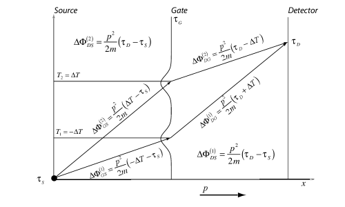
figure-images-xt-double-4\hyper@anchorend

The classic double slit experiment posits a single source that then shines through two slits.

The phase comes from the kinetic energy times the time. From source to gate we have:

\Hy@raisedlink\hyper@anchorstartequationxtdnullxtdouble6\hyper@anchorendΔΦGS=p22m(T1,2τS)\Hy@raisedlink\hyper@anchorstart𝑒𝑞𝑢𝑎𝑡𝑖𝑜𝑛𝑥𝑡𝑑𝑛𝑢𝑙𝑙𝑥𝑡𝑑𝑜𝑢𝑏𝑙𝑒6\hyper@anchorendΔsubscriptΦ𝐺𝑆superscript𝑝22𝑚subscript𝑇12subscript𝜏𝑆\Hy@raisedlink{\hyper@anchorstart{equation-xt-dnull-xt-double-6}\hyper@anchorend}\Delta{\Phi}_{GS}=\frac{{p}^{2}}{2m}\left({T}_{1,2}-{\tau}_{S}\right) (5.87)

And from gate to detector:

\Hy@raisedlink\hyper@anchorstartequationxtdnullxtdouble7\hyper@anchorendΔΦDG=p22m(τDT1,2)\Hy@raisedlink\hyper@anchorstart𝑒𝑞𝑢𝑎𝑡𝑖𝑜𝑛𝑥𝑡𝑑𝑛𝑢𝑙𝑙𝑥𝑡𝑑𝑜𝑢𝑏𝑙𝑒7\hyper@anchorendΔsubscriptΦ𝐷𝐺superscript𝑝22𝑚subscript𝜏𝐷subscript𝑇12\Hy@raisedlink{\hyper@anchorstart{equation-xt-dnull-xt-double-7}\hyper@anchorend}\Delta{\Phi}_{DG}=\frac{{p}^{2}}{2m}\left({\tau}_{D}-{T}_{1,2}\right) (5.88)

So, for a specific ray p, the total contribution of the kinetic energy to the phase is the same for either gate:

\Hy@raisedlink\hyper@anchorstartequationxtdnullxtdouble8\hyper@anchorendΔΦDS=ΔΦDG+ΔΦGS=p22mτDS\Hy@raisedlink\hyper@anchorstart𝑒𝑞𝑢𝑎𝑡𝑖𝑜𝑛𝑥𝑡𝑑𝑛𝑢𝑙𝑙𝑥𝑡𝑑𝑜𝑢𝑏𝑙𝑒8\hyper@anchorendΔsubscriptΦ𝐷𝑆ΔsubscriptΦ𝐷𝐺ΔsubscriptΦ𝐺𝑆superscript𝑝22𝑚subscript𝜏𝐷𝑆\Hy@raisedlink{\hyper@anchorstart{equation-xt-dnull-xt-double-8}\hyper@anchorend}\Delta{\Phi}_{DS}=\Delta{\Phi}_{DG}+\Delta{\Phi}_{GS}=\frac{{p}^{2}}{2m}{\tau}_{DS} (5.89)

Since we are associating each time ${\tau}_{\text{D}}$  at the detector with one ray p, the kinetic energy contribution to the phase will be the same whichever path we take 555We will see the same logic, with kinetic energy replaced by mass, when we look at the time part of the wave function in Double Slit in Temporal Quantization..

This does not eliminate all interference at the detector. Rays with different p  will interfere one with another. But it does mean that any interference pattern will be weak.

We therefore look at a more interesting case which is, in addition, a better fit to Lindner’s Attosecond Double Slit in Time. We model the double slit experiment in terms of two correlated sources. We look at the simplest possible approach: two free sources. We start the sources at ${\tau}_{S}^{\left(1,2\right)}=\mp\Delta T$  with identical distributions in momentum and quantum time, but with relative phase:

\Hy@raisedlink\hyper@anchorstartequationxtdnullxtdoublea\hyper@anchorendψG(1,2)exp(iϕ1,2),ϕ1,2=ϕ0Δϕformulae-sequencesimilar-to\Hy@raisedlink\hyper@anchorstart𝑒𝑞𝑢𝑎𝑡𝑖𝑜𝑛𝑥𝑡𝑑𝑛𝑢𝑙𝑙𝑥𝑡𝑑𝑜𝑢𝑏𝑙𝑒𝑎\hyper@anchorendsuperscriptsubscript𝜓𝐺12exp𝑖subscriptitalic-ϕ12subscriptitalic-ϕ12minus-or-plussubscriptitalic-ϕ0Δitalic-ϕ\Hy@raisedlink{\hyper@anchorstart{equation-xt-dnull-xt-double-a}\hyper@anchorend}{\psi}_{G}^{\left(1,2\right)}\sim\mathrm{exp}\left(-i{\phi}_{1,2}\right),{\phi}_{1,2}={\phi}_{0}\mp\Delta\phi (5.90)
5.2.4.2 Double Slit in Standard Quantum Theory
\Hy@raisedlink\hyper@anchorstart

xt-dsqt\hyper@anchorend

Refer to caption
Figure 5.4: Double Slit With Two Correlated Sources
\Hy@raisedlink
\hyper@anchorstart

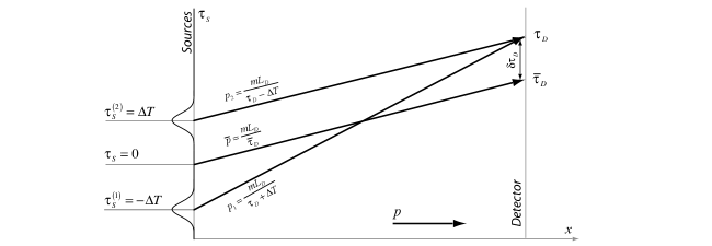
figure-images-xt-dtq-1\hyper@anchorend

We start with the wave function from the free case:

\Hy@raisedlink\hyper@anchorstartequationxtdsqtxtdsrcssqtxi12\hyper@anchorendξD(1,2)(δτD)=1πσ¯D24exp((δτD±ΔT)22σ¯D2ip¯22mτ¯D+ip¯22m(δτD±ΔT)+ip¯22m(δτD±ΔT)2τ¯Diϕ0±iΔϕ)\Hy@raisedlink\hyper@anchorstart𝑒𝑞𝑢𝑎𝑡𝑖𝑜𝑛𝑥𝑡𝑑𝑠𝑞𝑡𝑥𝑡𝑑𝑠𝑟𝑐𝑠𝑠𝑞𝑡𝑥𝑖12\hyper@anchorendsuperscriptsubscript𝜉𝐷12𝛿subscript𝜏𝐷41𝜋superscriptsubscript¯𝜎𝐷2expplus-or-minussuperscriptplus-or-minus𝛿subscript𝜏𝐷Δ𝑇22superscriptsubscript¯𝜎𝐷2𝑖superscript¯𝑝22𝑚subscript¯𝜏𝐷𝑖superscript¯𝑝22𝑚plus-or-minus𝛿subscript𝜏𝐷Δ𝑇𝑖superscript¯𝑝22𝑚superscriptplus-or-minus𝛿subscript𝜏𝐷Δ𝑇2subscript¯𝜏𝐷𝑖subscriptitalic-ϕ0𝑖Δitalic-ϕ\Hy@raisedlink{\hyper@anchorstart{equation-xt-dsqt-xt-dsrcs-sqt-xi12}\hyper@anchorend}{\xi}_{D}^{\left(1,2\right)}\left(\delta{\tau}_{D}\right)=\sqrt[4]{\frac{1}{\pi{\overline{\sigma}}_{D}^{2}}}\mathrm{exp}\left(-\frac{{\left(\delta{\tau}_{D}\pm\Delta T\right)}^{2}}{2{\overline{\sigma}}_{D}^{2}}-i\frac{{\overline{p}}^{2}}{2m}{\overline{\tau}}_{D}+i\frac{{\overline{p}}^{2}}{2m}\left(\delta{\tau}_{D}\pm\Delta T\right)+i\frac{{\overline{p}}^{2}}{2m}\frac{{\left(\delta{\tau}_{D}\pm\Delta T\right)}^{2}}{{\overline{\tau}}_{D}}-i{\phi}_{0}\pm i\Delta\phi\right) (5.91)

The full wave function is the sum of the terms from each gate:

\Hy@raisedlink\hyper@anchorstartequationxtdsqtxtdsrcssqt8\hyper@anchorendξD(δτD)=ξD(1)(δτD)+ξD(2)(δτD)\Hy@raisedlink\hyper@anchorstart𝑒𝑞𝑢𝑎𝑡𝑖𝑜𝑛𝑥𝑡𝑑𝑠𝑞𝑡𝑥𝑡𝑑𝑠𝑟𝑐𝑠𝑠𝑞𝑡8\hyper@anchorendsubscript𝜉𝐷𝛿subscript𝜏𝐷superscriptsubscript𝜉𝐷1𝛿subscript𝜏𝐷superscriptsubscript𝜉𝐷2𝛿subscript𝜏𝐷\Hy@raisedlink{\hyper@anchorstart{equation-xt-dsqt-xt-dsrcs-sqt-8}\hyper@anchorend}{\xi}_{D}\left(\delta{\tau}_{D}\right)={\xi}_{D}^{\left(1\right)}\left(\delta{\tau}_{D}\right)+{\xi}_{D}^{\left(2\right)}\left(\delta{\tau}_{D}\right) (5.92)

The probability density includes a normalization constant:

\Hy@raisedlink\hyper@anchorstartequationxtdsqtxtdsrcssqt9\hyper@anchorendρ¯D(δτD)=N¯2|ξD(1)(δτD)+ξD(2)(δτD)|2\Hy@raisedlink\hyper@anchorstart𝑒𝑞𝑢𝑎𝑡𝑖𝑜𝑛𝑥𝑡𝑑𝑠𝑞𝑡𝑥𝑡𝑑𝑠𝑟𝑐𝑠𝑠𝑞𝑡9\hyper@anchorendsubscript¯𝜌𝐷𝛿subscript𝜏𝐷superscript¯𝑁2superscriptsuperscriptsubscript𝜉𝐷1𝛿subscript𝜏𝐷superscriptsubscript𝜉𝐷2𝛿subscript𝜏𝐷2\Hy@raisedlink{\hyper@anchorstart{equation-xt-dsqt-xt-dsrcs-sqt-9}\hyper@anchorend}{\overline{\rho}}_{D}\left(\delta{\tau}_{D}\right)={\overline{N}}^{2}{\left|{\xi}_{D}^{\left(1\right)}\left(\delta{\tau}_{D}\right)+{\xi}_{D}^{\left(2\right)}\left(\delta{\tau}_{D}\right)\right|}^{2} (5.93)

Which is:

\Hy@raisedlink\hyper@anchorstartequationxtdsqtxtdsrcssqta\hyper@anchorendN¯2=1dτD|ξD(1)(δτD)+ξD(2)(δτD)|2\Hy@raisedlink\hyper@anchorstart𝑒𝑞𝑢𝑎𝑡𝑖𝑜𝑛𝑥𝑡𝑑𝑠𝑞𝑡𝑥𝑡𝑑𝑠𝑟𝑐𝑠𝑠𝑞𝑡𝑎\hyper@anchorendsuperscript¯𝑁21dsubscript𝜏𝐷superscriptsuperscriptsubscript𝜉𝐷1𝛿subscript𝜏𝐷superscriptsubscript𝜉𝐷2𝛿subscript𝜏𝐷2\Hy@raisedlink{\hyper@anchorstart{equation-xt-dsqt-xt-dsrcs-sqt-a}\hyper@anchorend}{\overline{N}}^{2}=\frac{1}{{\displaystyle\int\text{d}{\tau}_{D}{\left|{\xi}_{D}^{\left(1\right)}\left(\delta{\tau}_{D}\right)+{\xi}_{D}^{\left(2\right)}\left(\delta{\tau}_{D}\right)\right|}^{2}}} (5.94)

The probability density is given by three terms:

\Hy@raisedlink\hyper@anchorstartequationxtdsqtxtdsrcssqtb\hyper@anchorendρ¯D(δτD)=N¯2(ρ¯D(1)(δτD)+2ρ¯D(12)(δτD)+ρ¯D(2)(δτD))\Hy@raisedlink\hyper@anchorstart𝑒𝑞𝑢𝑎𝑡𝑖𝑜𝑛𝑥𝑡𝑑𝑠𝑞𝑡𝑥𝑡𝑑𝑠𝑟𝑐𝑠𝑠𝑞𝑡𝑏\hyper@anchorendsubscript¯𝜌𝐷𝛿subscript𝜏𝐷superscript¯𝑁2superscriptsubscript¯𝜌𝐷1𝛿subscript𝜏𝐷2superscriptsubscript¯𝜌𝐷tensor-product12𝛿subscript𝜏𝐷superscriptsubscript¯𝜌𝐷2𝛿subscript𝜏𝐷\Hy@raisedlink{\hyper@anchorstart{equation-xt-dsqt-xt-dsrcs-sqt-b}\hyper@anchorend}{\overline{\rho}}_{D}\left(\delta{\tau}_{D}\right)={\overline{N}}^{2}\left({\overline{\rho}}_{D}^{\left(1\right)}\left(\delta{\tau}_{D}\right)+2{\overline{\rho}}_{D}^{\left(1\otimes 2\right)}\left(\delta{\tau}_{D}\right)+{\overline{\rho}}_{D}^{\left(2\right)}\left(\delta{\tau}_{D}\right)\right) (5.95)

There are two outer humps, corresponding to each gate considered singly:

\Hy@raisedlink\hyper@anchorstartequationxtdsqtxtdsrcssqtc\hyper@anchorendρ¯D(1,2)(δτD)=ρ¯D(free)(δτD±ΔT)\Hy@raisedlink\hyper@anchorstart𝑒𝑞𝑢𝑎𝑡𝑖𝑜𝑛𝑥𝑡𝑑𝑠𝑞𝑡𝑥𝑡𝑑𝑠𝑟𝑐𝑠𝑠𝑞𝑡𝑐\hyper@anchorendsuperscriptsubscript¯𝜌𝐷12𝛿subscript𝜏𝐷superscriptsubscript¯𝜌𝐷𝑓𝑟𝑒𝑒plus-or-minus𝛿subscript𝜏𝐷Δ𝑇\Hy@raisedlink{\hyper@anchorstart{equation-xt-dsqt-xt-dsrcs-sqt-c}\hyper@anchorend}{\overline{\rho}}_{D}^{\left(1,2\right)}\left(\delta{\tau}_{D}\right)={\overline{\rho}}_{D}^{\left(free\right)}\left(\delta{\tau}_{D}\pm\Delta T\right) (5.96)

With:

\Hy@raisedlink\hyper@anchorstartequationxtdsqtxtdsrcssqtd\hyper@anchorendρ¯D(free)(δτD)=1πσ¯D2exp(δτD2σ¯D2)\Hy@raisedlink\hyper@anchorstart𝑒𝑞𝑢𝑎𝑡𝑖𝑜𝑛𝑥𝑡𝑑𝑠𝑞𝑡𝑥𝑡𝑑𝑠𝑟𝑐𝑠𝑠𝑞𝑡𝑑\hyper@anchorendsuperscriptsubscript¯𝜌𝐷𝑓𝑟𝑒𝑒𝛿subscript𝜏𝐷1𝜋superscriptsubscript¯𝜎𝐷2exp𝛿superscriptsubscript𝜏𝐷2superscriptsubscript¯𝜎𝐷2\Hy@raisedlink{\hyper@anchorstart{equation-xt-dsqt-xt-dsrcs-sqt-d}\hyper@anchorend}{\overline{\rho}}_{D}^{\left(free\right)}\left(\delta{\tau}_{D}\right)=\sqrt{\frac{1}{\pi{\overline{\sigma}}_{D}^{2}}}\mathrm{exp}\left(-\frac{\delta{\tau}_{D}^{2}}{{\overline{\sigma}}_{D}^{2}}\right) (5.97)

And a cross term in the middle:

\Hy@raisedlink\hyper@anchorstartequationxtdsqtxtdsrcssqtf\hyper@anchorendρ¯D(12)(δτD)=exp(ΔT2σ¯D2)cos(ϕ¯+f¯δτD)ρ¯D(free)(δτD)\Hy@raisedlink\hyper@anchorstart𝑒𝑞𝑢𝑎𝑡𝑖𝑜𝑛𝑥𝑡𝑑𝑠𝑞𝑡𝑥𝑡𝑑𝑠𝑟𝑐𝑠𝑠𝑞𝑡𝑓\hyper@anchorendsuperscriptsubscript¯𝜌𝐷tensor-product12𝛿subscript𝜏𝐷expΔsuperscript𝑇2superscriptsubscript¯𝜎𝐷2cos¯italic-ϕ¯𝑓𝛿subscript𝜏𝐷superscriptsubscript¯𝜌𝐷𝑓𝑟𝑒𝑒𝛿subscript𝜏𝐷\Hy@raisedlink{\hyper@anchorstart{equation-xt-dsqt-xt-dsrcs-sqt-f}\hyper@anchorend}{\overline{\rho}}_{D}^{\left(1\otimes 2\right)}\left(\delta{\tau}_{D}\right)=\mathrm{exp}\left(-\frac{\Delta{T}^{2}}{{\overline{\sigma}}_{D}^{2}}\right)\mathrm{cos}\left(\overline{\phi}+\overline{f}\delta{\tau}_{D}\right){\overline{\rho}}_{D}^{\left(free\right)}\left(\delta{\tau}_{D}\right) (5.98)

With frequency and angular offset:

\Hy@raisedlink\hyper@anchorstartequationxtdsqtxtdsrcssqtg\hyper@anchorendf¯4p¯22mΔTτ¯D\Hy@raisedlink\hyper@anchorstart𝑒𝑞𝑢𝑎𝑡𝑖𝑜𝑛𝑥𝑡𝑑𝑠𝑞𝑡𝑥𝑡𝑑𝑠𝑟𝑐𝑠𝑠𝑞𝑡𝑔\hyper@anchorend¯𝑓4superscript¯𝑝22𝑚Δ𝑇subscript¯𝜏𝐷\Hy@raisedlink{\hyper@anchorstart{equation-xt-dsqt-xt-dsrcs-sqt-g}\hyper@anchorend}\overline{f}\equiv 4\frac{{\overline{p}}^{2}}{2m}\frac{\Delta T}{{\overline{\tau}}_{D}} (5.99)
\Hy@raisedlink\hyper@anchorstartequationxtdsqtxtdsrcssqth\hyper@anchorendϕ¯2p¯22mΔT+2Δϕ\Hy@raisedlink\hyper@anchorstart𝑒𝑞𝑢𝑎𝑡𝑖𝑜𝑛𝑥𝑡𝑑𝑠𝑞𝑡𝑥𝑡𝑑𝑠𝑟𝑐𝑠𝑠𝑞𝑡\hyper@anchorend¯italic-ϕ2superscript¯𝑝22𝑚Δ𝑇2Δitalic-ϕ\Hy@raisedlink{\hyper@anchorstart{equation-xt-dsqt-xt-dsrcs-sqt-h}\hyper@anchorend}\overline{\phi}\equiv 2\frac{{\overline{p}}^{2}}{2m}\Delta T+2\Delta\phi (5.100)

Normalization:

\Hy@raisedlink\hyper@anchorstartequationxtdsqtxtdsrcssqti\hyper@anchorenddδτD(ρ¯D(1)(δτD)+2ρ¯D(12)(δτD)+ρ¯D(2)(δτD))=2+2exp(ΔT2σ¯D2f¯24σ¯D2)cos(ϕ¯)\Hy@raisedlink\hyper@anchorstart𝑒𝑞𝑢𝑎𝑡𝑖𝑜𝑛𝑥𝑡𝑑𝑠𝑞𝑡𝑥𝑡𝑑𝑠𝑟𝑐𝑠𝑠𝑞𝑡𝑖\hyper@anchorendd𝛿subscript𝜏𝐷superscriptsubscript¯𝜌𝐷1𝛿subscript𝜏𝐷2superscriptsubscript¯𝜌𝐷tensor-product12𝛿subscript𝜏𝐷superscriptsubscript¯𝜌𝐷2𝛿subscript𝜏𝐷22expΔsuperscript𝑇2superscriptsubscript¯𝜎𝐷2superscript¯𝑓24superscriptsubscript¯𝜎𝐷2cos¯italic-ϕ\Hy@raisedlink{\hyper@anchorstart{equation-xt-dsqt-xt-dsrcs-sqt-i}\hyper@anchorend}{\displaystyle\int\text{d}\delta{\tau}_{D}\left({\overline{\rho}}_{D}^{\left(1\right)}\left(\delta{\tau}_{D}\right)+2{\overline{\rho}}_{D}^{\left(1\otimes 2\right)}\left(\delta{\tau}_{D}\right)+{\overline{\rho}}_{D}^{\left(2\right)}\left(\delta{\tau}_{D}\right)\right)}=2+2\mathrm{exp}\left(-\frac{\Delta{T}^{2}}{{\overline{\sigma}}_{D}^{2}}-\frac{{\overline{f}}^{2}}{4}{\overline{\sigma}}_{D}^{2}\right)\mathrm{cos}\left(\overline{\phi}\right) (5.101)

Normalized probability density:

\Hy@raisedlink\hyper@anchorstartequationxtdsqtxtdsrcssqtk\hyper@anchorendρ¯D(δτD)=1πσ¯D2exp((δτD+ΔT)2σ¯D2)+2exp(δτD2+ΔT2σ¯D2)cos(ϕ¯+f¯δτD)+exp((δτDΔT)2σ¯D2)2+2exp(ΔT2σ¯D2f¯24σ¯D2)cos(ϕ¯)\Hy@raisedlink\hyper@anchorstart𝑒𝑞𝑢𝑎𝑡𝑖𝑜𝑛𝑥𝑡𝑑𝑠𝑞𝑡𝑥𝑡𝑑𝑠𝑟𝑐𝑠𝑠𝑞𝑡𝑘\hyper@anchorendsubscript¯𝜌𝐷𝛿subscript𝜏𝐷1𝜋superscriptsubscript¯𝜎𝐷2expsuperscript𝛿subscript𝜏𝐷Δ𝑇2superscriptsubscript¯𝜎𝐷22exp𝛿superscriptsubscript𝜏𝐷2Δsuperscript𝑇2superscriptsubscript¯𝜎𝐷2cos¯italic-ϕ¯𝑓𝛿subscript𝜏𝐷expsuperscript𝛿subscript𝜏𝐷Δ𝑇2superscriptsubscript¯𝜎𝐷222expΔsuperscript𝑇2superscriptsubscript¯𝜎𝐷2superscript¯𝑓24superscriptsubscript¯𝜎𝐷2cos¯italic-ϕ\Hy@raisedlink{\hyper@anchorstart{equation-xt-dsqt-xt-dsrcs-sqt-k}\hyper@anchorend}{\overline{\rho}}_{D}\left(\delta{\tau}_{D}\right)=\sqrt{\frac{1}{\pi{\overline{\sigma}}_{D}^{2}}}\frac{\mathrm{exp}\left(-\frac{{\left(\delta{\tau}_{D}+\Delta T\right)}^{2}}{{\overline{\sigma}}_{D}^{2}}\right)+2\mathrm{exp}\left(-\frac{\delta{\tau}_{D}^{2}+\Delta{T}^{2}}{{\overline{\sigma}}_{D}^{2}}\right)\mathrm{cos}\left(\overline{\phi}+\overline{f}\delta{\tau}_{D}\right)+\mathrm{exp}\left(-\frac{{\left(\delta{\tau}_{D}-\Delta T\right)}^{2}}{{\overline{\sigma}}_{D}^{2}}\right)}{2+2\mathrm{exp}\left(-\frac{\Delta{T}^{2}}{{\overline{\sigma}}_{D}^{2}}-\frac{{\overline{f}}^{2}}{4}{\overline{\sigma}}_{D}^{2}\right)\mathrm{cos}\left(\overline{\phi}\right)} (5.102)

When the initial sources are well-separated we see only the two outer humps. When they are closer together we see an interference pattern in the center.

5.2.4.3 Double Slit in Temporal Quantization
\Hy@raisedlink\hyper@anchorstart

xt-dtq\hyper@anchorend

We apply the same approach, using two free sources separated in time, to analyze the temporal quantization case. The two sources give:

\Hy@raisedlink\hyper@anchorstartequationxtdtqxtdsrcstq1\hyper@anchorendψD(1,2)(t,δp)=χD(1,2)(t,δp)ξD(1,2)(δp)\Hy@raisedlink\hyper@anchorstart𝑒𝑞𝑢𝑎𝑡𝑖𝑜𝑛𝑥𝑡𝑑𝑡𝑞𝑥𝑡𝑑𝑠𝑟𝑐𝑠𝑡𝑞1\hyper@anchorendsuperscriptsubscript𝜓𝐷12𝑡𝛿𝑝superscriptsubscript𝜒𝐷12𝑡𝛿𝑝superscriptsubscript𝜉𝐷12𝛿𝑝\Hy@raisedlink{\hyper@anchorstart{equation-xt-dtq-xt-dsrcs-tq-1}\hyper@anchorend}{\psi}_{D}^{\left(1,2\right)}\left(t,\delta p\right)={\chi}_{D}^{\left(1,2\right)}\left(t,\delta p\right){\xi}_{D}^{\left(1,2\right)}\left(\delta p\right) (5.103)

With time parts:

\Hy@raisedlink\hyper@anchorstartequationxtdtqxtdsrcstq2\hyper@anchorendχD(1,2)(t,δp)=1πσ02fD(0)24exp(iE¯1,2tDtD22σ02fD(0)im(τD±ΔT))\Hy@raisedlink\hyper@anchorstart𝑒𝑞𝑢𝑎𝑡𝑖𝑜𝑛𝑥𝑡𝑑𝑡𝑞𝑥𝑡𝑑𝑠𝑟𝑐𝑠𝑡𝑞2\hyper@anchorendsuperscriptsubscript𝜒𝐷12𝑡𝛿𝑝41𝜋superscriptsubscript𝜎02superscriptsubscript𝑓𝐷02exp𝑖subscript¯𝐸12subscript𝑡𝐷superscriptsubscript𝑡𝐷22superscriptsubscript𝜎02superscriptsubscript𝑓𝐷0𝑖𝑚plus-or-minussubscript𝜏𝐷Δ𝑇\Hy@raisedlink{\hyper@anchorstart{equation-xt-dtq-xt-dsrcs-tq-2}\hyper@anchorend}{\chi}_{D}^{\left(1,2\right)}\left(t,\delta p\right)=\sqrt[4]{\frac{1}{\pi{\sigma}_{0}^{2}{f}_{D}^{\left(0\right)2}}}\mathrm{exp}\left(-i{\overline{E}}_{1,2}{t}_{D}-\frac{{t}_{D}^{2}}{2{\sigma}_{0}^{2}{f}_{D}^{\left(0\right)}}-im\left({\tau}_{D}\pm\Delta T\right)\right) (5.104)

And space parts:

\Hy@raisedlink\hyper@anchorstartequationxtdtqxtdsrcstq3\hyper@anchorendξ^D(1,2)(δp)=1πσ^124exp(δp22σ^12)exp(ip22m(τD±ΔT)iϕ1,2)\Hy@raisedlink\hyper@anchorstart𝑒𝑞𝑢𝑎𝑡𝑖𝑜𝑛𝑥𝑡𝑑𝑡𝑞𝑥𝑡𝑑𝑠𝑟𝑐𝑠𝑡𝑞3\hyper@anchorendsuperscriptsubscript^𝜉𝐷12𝛿𝑝41𝜋superscriptsubscript^𝜎12exp𝛿superscript𝑝22superscriptsubscript^𝜎12exp𝑖superscript𝑝22𝑚plus-or-minussubscript𝜏𝐷Δ𝑇𝑖subscriptitalic-ϕ12\Hy@raisedlink{\hyper@anchorstart{equation-xt-dtq-xt-dsrcs-tq-3}\hyper@anchorend}{\widehat{\xi}}_{D}^{\left(1,2\right)}\left(\delta p\right)=\sqrt[4]{\frac{1}{\pi{\widehat{\sigma}}_{1}^{2}}}\mathrm{exp}\left(-\frac{\delta{p}^{2}}{2{\widehat{\sigma}}_{1}^{2}}\right)\mathrm{exp}\left(-i\frac{{p}^{2}}{2m}\left({\tau}_{D}\pm\Delta T\right)-i{\phi}_{1,2}\right) (5.105)
Probability Density in Time and Space

If we imagine a pencil beam coming from each of our two gates, aimed at a specific point, it will take sharply different momenta to arrive at the detector at the same ${\tau}_{\text{D}}$:

\Hy@raisedlink\hyper@anchorstartequationxtdtqxtdsrcspoint0\hyper@anchorendτD=mLDp1ΔT=mLDp2+ΔT\Hy@raisedlink\hyper@anchorstart𝑒𝑞𝑢𝑎𝑡𝑖𝑜𝑛𝑥𝑡𝑑𝑡𝑞𝑥𝑡𝑑𝑠𝑟𝑐𝑠𝑝𝑜𝑖𝑛𝑡0\hyper@anchorendsubscript𝜏𝐷𝑚subscript𝐿𝐷subscript𝑝1Δ𝑇𝑚subscript𝐿𝐷subscript𝑝2Δ𝑇\Hy@raisedlink{\hyper@anchorstart{equation-xt-dtq-xt-dsrcs-point-0}\hyper@anchorend}{\tau}_{D}=\frac{m{L}_{D}}{{p}_{1}}-\Delta T=\frac{m{L}_{D}}{{p}_{2}}+\Delta T (5.106)

Implying (working as usual only to first order):

\Hy@raisedlink\hyper@anchorstartequationxtdtqxtdsrcspoint1\hyper@anchorendp1,2=mLDτD±ΔT=mLDτ¯D+δτD±ΔT=p¯(1δτD±ΔTτ¯D)δp1,2=δτD±ΔTτ¯Dp¯\Hy@raisedlink\hyper@anchorstart𝑒𝑞𝑢𝑎𝑡𝑖𝑜𝑛𝑥𝑡𝑑𝑡𝑞𝑥𝑡𝑑𝑠𝑟𝑐𝑠𝑝𝑜𝑖𝑛𝑡1\hyper@anchorendsubscript𝑝12𝑚subscript𝐿𝐷plus-or-minussubscript𝜏𝐷Δ𝑇𝑚subscript𝐿𝐷plus-or-minussubscript¯𝜏𝐷𝛿subscript𝜏𝐷Δ𝑇¯𝑝1plus-or-minus𝛿subscript𝜏𝐷Δ𝑇subscript¯𝜏𝐷𝛿subscript𝑝12plus-or-minus𝛿subscript𝜏𝐷Δ𝑇subscript¯𝜏𝐷¯𝑝\Hy@raisedlink{\hyper@anchorstart{equation-xt-dtq-xt-dsrcs-point-1}\hyper@anchorend}{p}_{1,2}=\frac{m{L}_{D}}{{\tau}_{D}\pm\Delta T}=\frac{m{L}_{D}}{{\overline{\tau}}_{D}+\delta{\tau}_{D}\pm\Delta T}=\overline{p}\left(1-\frac{\delta{\tau}_{D}\pm\Delta T}{{\overline{\tau}}_{D}}\right)\Rightarrow\delta{p}_{1,2}=-\frac{\delta{\tau}_{D}\pm\Delta T}{{\overline{\tau}}_{D}}\overline{p} (5.107)

These shifts give us, not surprisingly, the previous standard quantum theory wave functions:

\Hy@raisedlink\hyper@anchorstartequationxtdtqxtdsrcssqtxi12\hyper@anchorendξD(1,2)(δτD)=1πσ¯D24exp((δτD±ΔT)22σ¯D2ip¯22mτ¯D+ip¯22m(δτD±ΔT)+ip¯22m(δτD±ΔT)2τ¯Diϕ0±iΔϕ)\Hy@raisedlink\hyper@anchorstart𝑒𝑞𝑢𝑎𝑡𝑖𝑜𝑛𝑥𝑡𝑑𝑡𝑞𝑥𝑡𝑑𝑠𝑟𝑐𝑠𝑠𝑞𝑡𝑥𝑖12\hyper@anchorendsuperscriptsubscript𝜉𝐷12𝛿subscript𝜏𝐷41𝜋superscriptsubscript¯𝜎𝐷2expplus-or-minussuperscriptplus-or-minus𝛿subscript𝜏𝐷Δ𝑇22superscriptsubscript¯𝜎𝐷2𝑖superscript¯𝑝22𝑚subscript¯𝜏𝐷𝑖superscript¯𝑝22𝑚plus-or-minus𝛿subscript𝜏𝐷Δ𝑇𝑖superscript¯𝑝22𝑚superscriptplus-or-minus𝛿subscript𝜏𝐷Δ𝑇2subscript¯𝜏𝐷𝑖subscriptitalic-ϕ0𝑖Δitalic-ϕ\Hy@raisedlink{\hyper@anchorstart{equation-xt-dtq-xt-dsrcs-sqt-xi12}\hyper@anchorend}{\xi}_{D}^{\left(1,2\right)}\left(\delta{\tau}_{D}\right)=\sqrt[4]{\frac{1}{\pi{\overline{\sigma}}_{D}^{2}}}\mathrm{exp}\left(-\frac{{\left(\delta{\tau}_{D}\pm\Delta T\right)}^{2}}{2{\overline{\sigma}}_{D}^{2}}-i\frac{{\overline{p}}^{2}}{2m}{\overline{\tau}}_{D}+i\frac{{\overline{p}}^{2}}{2m}\left(\delta{\tau}_{D}\pm\Delta T\right)+i\frac{{\overline{p}}^{2}}{2m}\frac{{\left(\delta{\tau}_{D}\pm\Delta T\right)}^{2}}{{\overline{\tau}}_{D}}-i{\phi}_{0}\pm i\Delta\phi\right) (5.108)

In the time part of the wave function we have still to consider the factor $\mathrm{exp}\left(\mp im\Delta T\right)$.

We make the same argument as was made earlier with respect to the non-interference in the single source case (Relative Lack of Interference in the Simplest Case). The part of the wave function going through the first gate gets a total phase:

\Hy@raisedlink\hyper@anchorstartequationxtdtqxtdsrcspoint4\hyper@anchorendm(ΔTτS)m(τD+ΔT)\Hy@raisedlink\hyper@anchorstart𝑒𝑞𝑢𝑎𝑡𝑖𝑜𝑛𝑥𝑡𝑑𝑡𝑞𝑥𝑡𝑑𝑠𝑟𝑐𝑠𝑝𝑜𝑖𝑛𝑡4\hyper@anchorend𝑚Δ𝑇subscript𝜏𝑆𝑚subscript𝜏𝐷Δ𝑇\Hy@raisedlink{\hyper@anchorstart{equation-xt-dtq-xt-dsrcs-point-4}\hyper@anchorend}-m\left(-\Delta T-{\tau}_{S}\right)-m\left({\tau}_{D}+\Delta T\right) (5.109)

The second:

\Hy@raisedlink\hyper@anchorstartequationxtdtqxtdsrcspoint5\hyper@anchorendm(ΔTτS)m(τDΔT)\Hy@raisedlink\hyper@anchorstart𝑒𝑞𝑢𝑎𝑡𝑖𝑜𝑛𝑥𝑡𝑑𝑡𝑞𝑥𝑡𝑑𝑠𝑟𝑐𝑠𝑝𝑜𝑖𝑛𝑡5\hyper@anchorend𝑚Δ𝑇subscript𝜏𝑆𝑚subscript𝜏𝐷Δ𝑇\Hy@raisedlink{\hyper@anchorstart{equation-xt-dtq-xt-dsrcs-point-5}\hyper@anchorend}-m\left(\Delta T-{\tau}_{S}\right)-m\left({\tau}_{D}-\Delta T\right) (5.110)

These are equal so irrelevant. Formally, we can absorb these phases into the angle:

\Hy@raisedlink\hyper@anchorstartequationxtdtqxtdsrcspoint6\hyper@anchorendϕ1ϕ1+m(ΔTτS)ϕ2ϕ2+m(ΔTτS)\Hy@raisedlink\hyper@anchorstart𝑒𝑞𝑢𝑎𝑡𝑖𝑜𝑛𝑥𝑡𝑑𝑡𝑞𝑥𝑡𝑑𝑠𝑟𝑐𝑠𝑝𝑜𝑖𝑛𝑡6\hyper@anchorendsubscriptitalic-ϕ1subscriptitalic-ϕ1𝑚Δ𝑇subscript𝜏𝑆subscriptitalic-ϕ2subscriptitalic-ϕ2𝑚Δ𝑇subscript𝜏𝑆\Hy@raisedlink{\hyper@anchorstart{equation-xt-dtq-xt-dsrcs-point-6}\hyper@anchorend}\begin{array}[]{l}{\phi}_{1}\rightarrow{\phi}_{1}+m\left(-\Delta T-{\tau}_{S}\right)\\ {\phi}_{2}\rightarrow{\phi}_{2}+m\left(\Delta T-{\tau}_{S}\right)\end{array} (5.111)

The probability density in time and space is now:

\Hy@raisedlink\hyper@anchorstartequationxtdtqxtdsrcspdens0\hyper@anchorendρD(tD,δτD)=|ψD(1)(tD,δτD)+ψD(2)(tD,δτD)|2\Hy@raisedlink\hyper@anchorstart𝑒𝑞𝑢𝑎𝑡𝑖𝑜𝑛𝑥𝑡𝑑𝑡𝑞𝑥𝑡𝑑𝑠𝑟𝑐𝑠𝑝𝑑𝑒𝑛𝑠0\hyper@anchorendsubscript𝜌𝐷subscript𝑡𝐷𝛿subscript𝜏𝐷superscriptsuperscriptsubscript𝜓𝐷1subscript𝑡𝐷𝛿subscript𝜏𝐷superscriptsubscript𝜓𝐷2subscript𝑡𝐷𝛿subscript𝜏𝐷2\Hy@raisedlink{\hyper@anchorstart{equation-xt-dtq-xt-dsrcs-pdens-0}\hyper@anchorend}{\rho}_{D}\left({t}_{D},\delta{\tau}_{D}\right)={\left|{\psi}_{D}^{\left(1\right)}\left({t}_{D},\delta{\tau}_{D}\right)+{\psi}_{D}^{\left(2\right)}\left({t}_{D},\delta{\tau}_{D}\right)\right|}^{2} (5.112)

There are three terms as before:

\Hy@raisedlink\hyper@anchorstartequationxtdtqxtdsrcspdens1\hyper@anchorendρD(tD,δτD)=ρD(1)(tD,δτD)+2ρD(12)(tD,δτD)+ρD(2)(tD,δτD)\Hy@raisedlink\hyper@anchorstart𝑒𝑞𝑢𝑎𝑡𝑖𝑜𝑛𝑥𝑡𝑑𝑡𝑞𝑥𝑡𝑑𝑠𝑟𝑐𝑠𝑝𝑑𝑒𝑛𝑠1\hyper@anchorendsubscript𝜌𝐷subscript𝑡𝐷𝛿subscript𝜏𝐷superscriptsubscript𝜌𝐷1subscript𝑡𝐷𝛿subscript𝜏𝐷2superscriptsubscript𝜌𝐷tensor-product12subscript𝑡𝐷𝛿subscript𝜏𝐷superscriptsubscript𝜌𝐷2subscript𝑡𝐷𝛿subscript𝜏𝐷\Hy@raisedlink{\hyper@anchorstart{equation-xt-dtq-xt-dsrcs-pdens-1}\hyper@anchorend}{\rho}_{D}\left({t}_{D},\delta{\tau}_{D}\right)={\rho}_{D}^{\left(1\right)}\left({t}_{D},\delta{\tau}_{D}\right)+2{\rho}_{D}^{\left(1\otimes 2\right)}\left({t}_{D},\delta{\tau}_{D}\right)+{\rho}_{D}^{\left(2\right)}\left({t}_{D},\delta{\tau}_{D}\right) (5.113)

The outer humps are:

\Hy@raisedlink\hyper@anchorstartequationxtdtqxtdsrcspdens2\hyper@anchorendρD(1,2)(tD,δτD)=ρD(free)(tD,δτD)ρ¯D(free)(δτ±ΔT)\Hy@raisedlink{\hyper@anchorstart{equation-xt-dtq-xt-dsrcs-pdens-2}\hyper@anchorend}{\rho}_{D}^{\left(1,2\right)}\left({t}_{D},\delta{\tau}_{D}\right)={\stackrel{{\scriptstyle\frown}}{{\rho}}}_{D}^{\left(free\right)}\left({t}_{D},\delta{\tau}_{D}\right){\overline{\rho}}_{D}^{\left(free\right)}\left(\delta\tau\pm\Delta T\right) (5.114)

With:

\Hy@raisedlink\hyper@anchorstartequationxtdtqxtdsrcspdens3\hyper@anchorendρD(free)(tD,δτD)=1πσ02|fD(0)|2exp(tD2σ02|fD(0)|2)superscriptsubscriptsuperscript𝜌𝐷𝑓𝑟𝑒𝑒\Hy@raisedlink\hyper@anchorstart𝑒𝑞𝑢𝑎𝑡𝑖𝑜𝑛𝑥𝑡𝑑𝑡𝑞𝑥𝑡𝑑𝑠𝑟𝑐𝑠𝑝𝑑𝑒𝑛𝑠3\hyper@anchorendsubscript𝑡𝐷𝛿subscript𝜏𝐷1𝜋superscriptsubscript𝜎02superscriptsuperscriptsubscript𝑓𝐷02expsuperscriptsubscript𝑡𝐷2superscriptsubscript𝜎02superscriptsuperscriptsubscript𝑓𝐷02\Hy@raisedlink{\hyper@anchorstart{equation-xt-dtq-xt-dsrcs-pdens-3}\hyper@anchorend}{\stackrel{{\scriptstyle\frown}}{{\rho}}}_{D}^{\left(free\right)}\left({t}_{D},\delta{\tau}_{D}\right)=\sqrt{\frac{1}{\pi{\sigma}_{0}^{2}{\left|{f}_{D}^{\left(0\right)}\right|}^{2}}}\mathrm{exp}\left(-\frac{{t}_{D}^{2}}{{\sigma}_{0}^{2}{\left|{f}_{D}^{\left(0\right)}\right|}^{2}}\right) (5.115)

The cross term is now:

\Hy@raisedlink\hyper@anchorstartequationxtdtqxtdsrcspdens5\hyper@anchorendρD(12)(tD,δτD)=12ρD(free)(tD,δτD)(ξD(1)(δτD+ΔT)ξD(2)(δτDΔT)+ξD(1)(δτD+ΔT)ξD(2)(δτDΔT))\Hy@raisedlink\hyper@anchorstart𝑒𝑞𝑢𝑎𝑡𝑖𝑜𝑛𝑥𝑡𝑑𝑡𝑞𝑥𝑡𝑑𝑠𝑟𝑐𝑠𝑝𝑑𝑒𝑛𝑠5\hyper@anchorendsuperscriptsubscript𝜌𝐷tensor-product12subscript𝑡𝐷𝛿subscript𝜏𝐷12superscriptsubscriptsuperscript𝜌𝐷𝑓𝑟𝑒𝑒subscript𝑡𝐷𝛿subscript𝜏𝐷superscriptsubscript𝜉𝐷1𝛿subscript𝜏𝐷Δ𝑇superscriptsubscript𝜉𝐷2𝛿subscript𝜏𝐷Δ𝑇superscriptsubscript𝜉𝐷1𝛿subscript𝜏𝐷Δ𝑇superscriptsubscript𝜉𝐷2𝛿subscript𝜏𝐷Δ𝑇\Hy@raisedlink{\hyper@anchorstart{equation-xt-dtq-xt-dsrcs-pdens-5}\hyper@anchorend}{\rho}_{D}^{\left(1\otimes 2\right)}\left({t}_{D},\delta{\tau}_{D}\right)=\frac{1}{2}{\stackrel{{\scriptstyle\frown}}{{\rho}}}_{D}^{\left(free\right)}\left({t}_{D},\delta{\tau}_{D}\right)\left({\xi}_{D}^{\left(1\right)\ast}\left(\delta{\tau}_{D}+\Delta T\right){\xi}_{D}^{\left(2\right)}\left(\delta{\tau}_{D}-\Delta T\right)+{\xi}_{D}^{\left(1\right)}\left(\delta{\tau}_{D}+\Delta T\right){\xi}_{D}^{\left(2\right)\ast}\left(\delta{\tau}_{D}-\Delta T\right)\right) (5.116)

Which is the free quantum time wave function times the momentum space cross term.

Therefore we can factor out the probability density in time from the total probability density 666 If we had generalized the dispersion in time to include dependence on momentum ${\sigma}_{0}^{2}\rightarrow{\sigma}_{0}^{2}\left(p\right)$  or had taken $\gamma>1$  we would not have been able to factor out the time part. :

\Hy@raisedlink\hyper@anchorstartequationxtdtqxtdsrcspdens7\hyper@anchorendρD(t,δτD)=ρD(free)(tD,δτD)ρ¯D(δτD)\Hy@raisedlink{\hyper@anchorstart{equation-xt-dtq-xt-dsrcs-pdens-7}\hyper@anchorend}{\rho}_{D}\left(t,\delta{\tau}_{D}\right)={\stackrel{{\scriptstyle\frown}}{{\rho}}}_{D}^{\left(free\right)}\left({t}_{D},\delta{\tau}_{D}\right){\overline{\rho}}_{D}\left(\delta{\tau}_{D}\right) (5.117)
Probability Density in Time Only

The probability density in time only is given by:

\Hy@raisedlink\hyper@anchorstartequationxtdtqxtdsrcsfinal1\hyper@anchorendρD(tD¯)=dδτDρD(tD,δτD)ρ¯D(δτD)\Hy@raisedlink\hyper@anchorstart𝑒𝑞𝑢𝑎𝑡𝑖𝑜𝑛𝑥𝑡𝑑𝑡𝑞𝑥𝑡𝑑𝑠𝑟𝑐𝑠𝑓𝑖𝑛𝑎𝑙1\hyper@anchorendsubscript𝜌𝐷subscript𝑡¯𝐷d𝛿subscript𝜏𝐷subscriptsuperscript𝜌𝐷subscript𝑡𝐷𝛿subscript𝜏𝐷subscript¯𝜌𝐷𝛿subscript𝜏𝐷\Hy@raisedlink{\hyper@anchorstart{equation-xt-dtq-xt-dsrcs-final-1}\hyper@anchorend}{\rho}_{D}\left({t}_{\overline{D}}\right)={\displaystyle\int\text{d}\delta{\tau}_{D}{\stackrel{{\scriptstyle\frown}}{{\rho}}}_{D}\left({t}_{D},\delta{\tau}_{D}\right){\overline{\rho}}_{D}\left(\delta{\tau}_{D}\right)} (5.118)

Explicitly:

\Hy@raisedlink\hyper@anchorstartequationxtdtqxtdsrcsfinal1b\hyper@anchorendρD(tD¯)=dδτD1πσD2exp((tD¯δτD)2σD2)1πσ¯D2(exp((δτD+ΔT)2σ¯D2)+2exp(δτD2+ΔT2σ¯D2)cos(ϕ¯+f¯δτD)+exp((δτDΔT)2σ¯D2))\Hy@raisedlink\hyper@anchorstart𝑒𝑞𝑢𝑎𝑡𝑖𝑜𝑛𝑥𝑡𝑑𝑡𝑞𝑥𝑡𝑑𝑠𝑟𝑐𝑠𝑓𝑖𝑛𝑎𝑙1𝑏\hyper@anchorendsubscript𝜌𝐷subscript𝑡¯𝐷d𝛿subscript𝜏𝐷1superscriptsubscriptsuperscript𝜎𝐷2𝜋absentexpsuperscriptsubscript𝑡¯𝐷𝛿subscript𝜏𝐷2superscriptsubscriptsuperscript𝜎𝐷21𝜋superscriptsubscript¯𝜎𝐷2expsuperscript𝛿subscript𝜏𝐷Δ𝑇2superscriptsubscript¯𝜎𝐷22exp𝛿superscriptsubscript𝜏𝐷2Δsuperscript𝑇2superscriptsubscript¯𝜎𝐷2cos¯italic-ϕ¯𝑓𝛿subscript𝜏𝐷expsuperscript𝛿subscript𝜏𝐷Δ𝑇2superscriptsubscript¯𝜎𝐷2\Hy@raisedlink{\hyper@anchorstart{equation-xt-dtq-xt-dsrcs-final-1b}\hyper@anchorend}{\rho}_{D}\left({t}_{\overline{D}}\right)={\displaystyle\int\text{d}\delta{\tau}_{D}\sqrt{\frac{1}{\pi{\stackrel{{\scriptstyle\frown}}{{\sigma}}}_{D}^{2}}}\mathrm{exp}\left(-\frac{{\left({t}_{\overline{D}}-\delta{\tau}_{D}\right)}^{2}}{{\stackrel{{\scriptstyle\frown}}{{\sigma}}}_{D}^{2}}\right)\sqrt{\frac{1}{\pi{\overline{\sigma}}_{D}^{2}}}\left(\begin{array}[]{l}\mathrm{exp}\left(-\frac{{\left(\delta{\tau}_{D}+\Delta T\right)}^{2}}{{\overline{\sigma}}_{D}^{2}}\right)\\ +2\mathrm{exp}\left(-\frac{\delta{\tau}_{D}^{2}+\Delta{T}^{2}}{{\overline{\sigma}}_{D}^{2}}\right)\mathrm{cos}\left(\overline{\phi}+\overline{f}\delta{\tau}_{D}\right)\\ +\mathrm{exp}\left(-\frac{{\left(\delta{\tau}_{D}-\Delta T\right)}^{2}}{{\overline{\sigma}}_{D}^{2}}\right)\end{array}\right)} (5.119)

Giving:

\Hy@raisedlink\hyper@anchorstartequationxtdtqxtdsrcsfinal2\hyper@anchorendρD(tD¯)=(1πσD2exp((tD¯+ΔT)2σD2)+2exp(ΔT2σ¯D2σD2σ¯D24σD2f¯2)cos(ϕ¯+σ¯D2σD2+σ¯D2f¯tD¯)1πσD2exp(tD¯2σD2)+1πσD2exp((tD¯ΔT)2σD2))\Hy@raisedlink\hyper@anchorstart𝑒𝑞𝑢𝑎𝑡𝑖𝑜𝑛𝑥𝑡𝑑𝑡𝑞𝑥𝑡𝑑𝑠𝑟𝑐𝑠𝑓𝑖𝑛𝑎𝑙2\hyper@anchorendsubscript𝜌𝐷subscript𝑡¯𝐷1𝜋superscriptsubscript𝜎𝐷2expsuperscriptsubscript𝑡¯𝐷Δ𝑇2superscriptsubscript𝜎𝐷22expΔsuperscript𝑇2superscriptsubscript¯𝜎𝐷2superscriptsubscriptsuperscript𝜎𝐷2absentsuperscriptsubscript¯𝜎𝐷24superscriptsubscript𝜎𝐷2superscript¯𝑓2cos¯italic-ϕsuperscriptsubscript¯𝜎𝐷2superscriptsubscriptsuperscript𝜎𝐷2absentsuperscriptsubscript¯𝜎𝐷2¯𝑓subscript𝑡¯𝐷1𝜋superscriptsubscript𝜎𝐷2expsuperscriptsubscript𝑡¯𝐷2superscriptsubscript𝜎𝐷21𝜋superscriptsubscript𝜎𝐷2expsuperscriptsubscript𝑡¯𝐷Δ𝑇2superscriptsubscript𝜎𝐷2\Hy@raisedlink{\hyper@anchorstart{equation-xt-dtq-xt-dsrcs-final-2}\hyper@anchorend}{\rho}_{D}\left({t}_{\overline{D}}\right)=\left(\begin{array}[]{l}\sqrt{\frac{1}{\pi{\sigma}_{D}^{2}}}\mathrm{exp}\left(-\frac{{\left({t}_{\overline{D}}+\Delta T\right)}^{2}}{{\sigma}_{D}^{2}}\right)\\ +2\mathrm{exp}\left(-\frac{\Delta{T}^{2}}{{\overline{\sigma}}_{D}^{2}}-\frac{{\stackrel{{\scriptstyle\frown}}{{\sigma}}}_{D}^{2}{\overline{\sigma}}_{D}^{2}}{4{\sigma}_{D}^{2}}{\overline{f}}^{2}\right)\mathrm{cos}\left(\overline{\phi}+\frac{{\overline{\sigma}}_{D}^{2}}{{\stackrel{{\scriptstyle\frown}}{{\sigma}}}_{D}^{2}+{\overline{\sigma}}_{D}^{2}}\overline{f}{t}_{\overline{D}}\right)\sqrt{\frac{1}{\pi{\sigma}_{D}^{2}}}\mathrm{exp}\left(-\frac{{t}_{\overline{D}}^{2}}{{\sigma}_{D}^{2}}\right)\\ +\sqrt{\frac{1}{\pi{\sigma}_{D}^{2}}}\mathrm{exp}\left(-\frac{{\left({t}_{\overline{D}}-\Delta T\right)}^{2}}{{\sigma}_{D}^{2}}\right)\end{array}\right) (5.120)

The effects of temporal quantization are three:

  1. 1.

    All three humps are widened by the familiar factor:

    \Hy@raisedlink\hyper@anchorstartequationxtdtqxtdsrcsfinal3\hyper@anchorendσ¯D2σD2=σD2+σ¯D2\Hy@raisedlink{\hyper@anchorstart{equation-xt-dtq-xt-dsrcs-final-3}\hyper@anchorend}{\overline{\sigma}}_{D}^{2}\rightarrow{\sigma}_{D}^{2}={\stackrel{{\scriptstyle\frown}}{{\sigma}}}_{D}^{2}+{\overline{\sigma}}_{D}^{2} (5.121)
  2. 2.

    The frequency is reduced:

    \Hy@raisedlink\hyper@anchorstartequationxtdtqxtdsrcsfinal4\hyper@anchorendf¯σ¯D2σD2+σ¯D2f¯\Hy@raisedlink\hyper@anchorstart𝑒𝑞𝑢𝑎𝑡𝑖𝑜𝑛𝑥𝑡𝑑𝑡𝑞𝑥𝑡𝑑𝑠𝑟𝑐𝑠𝑓𝑖𝑛𝑎𝑙4\hyper@anchorend¯𝑓superscriptsubscript¯𝜎𝐷2superscriptsubscriptsuperscript𝜎𝐷2absentsuperscriptsubscript¯𝜎𝐷2¯𝑓\Hy@raisedlink{\hyper@anchorstart{equation-xt-dtq-xt-dsrcs-final-4}\hyper@anchorend}\overline{f}\rightarrow\frac{{\overline{\sigma}}_{D}^{2}}{{\stackrel{{\scriptstyle\frown}}{{\sigma}}}_{D}^{2}+{\overline{\sigma}}_{D}^{2}}\overline{f} (5.122)
  3. 3.

    The central hump is suppressed:

    \Hy@raisedlink\hyper@anchorstartequationxtdtqxtdsrcsfinal5\hyper@anchorendexp(ΔT2σ¯D2)exp(ΔT2σ¯D2σD2σ¯D24σD2f¯2)\Hy@raisedlink\hyper@anchorstart𝑒𝑞𝑢𝑎𝑡𝑖𝑜𝑛𝑥𝑡𝑑𝑡𝑞𝑥𝑡𝑑𝑠𝑟𝑐𝑠𝑓𝑖𝑛𝑎𝑙5\hyper@anchorendexpΔsuperscript𝑇2superscriptsubscript¯𝜎𝐷2expΔsuperscript𝑇2superscriptsubscript¯𝜎𝐷2superscriptsubscriptsuperscript𝜎𝐷2absentsuperscriptsubscript¯𝜎𝐷24superscriptsubscript𝜎𝐷2superscript¯𝑓2\Hy@raisedlink{\hyper@anchorstart{equation-xt-dtq-xt-dsrcs-final-5}\hyper@anchorend}\mathrm{exp}\left(-\frac{\Delta{T}^{2}}{{\overline{\sigma}}_{D}^{2}}\right)\rightarrow\mathrm{exp}\left(-\frac{\Delta{T}^{2}}{{\overline{\sigma}}_{D}^{2}}-\frac{{\stackrel{{\scriptstyle\frown}}{{\sigma}}}_{D}^{2}{\overline{\sigma}}_{D}^{2}}{4{\sigma}_{D}^{2}}{\overline{f}}^{2}\right) (5.123)

Essentially each individual crest is widened while the oscillatory "comb" is stretched out and flattened at the same time.

5.2.5 Attosecond Double Slit in Time

\Hy@raisedlink\hyper@anchorstart

xt-lind\hyper@anchorend

5.2.5.1 Overview
\Hy@raisedlink\hyper@anchorstart

xt-linintro\hyper@anchorend

Refer to caption
Figure 5.5: Electric Field as Source
\Hy@raisedlink
\hyper@anchorstart

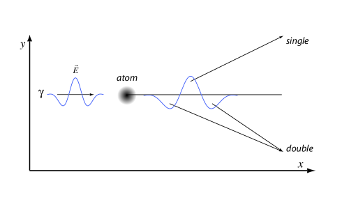
figure-images-xt-lind-4\hyper@anchorend

In Lindner et al’s 2005 experiment Attosecond Double Slit in Time [734], a strong short electric pulse ionizes a bound electron. Like water shaken off by a dog, the electron can come off to right or left.

The pulses are extremely short, with one hump on one side, two on the other. If the electron is shaken off by the one humped side, we have a single slit experiment. If the electron is shaken off by the two humped side, we have a double slit experiment: the wave functions generated by the two humps will interfere with each other.

The experiment itself is one of those that put the "non" into "nontrivial"; the associated calculations are difficult as well. We will therefore look only at an extremely simplified model of the Lindner experiment.

5.2.5.2 Model Experiment
\Hy@raisedlink\hyper@anchorstart

xt-linmodel\hyper@anchorend

Electric Field

We take a photon going from left to right in x  direction, with an electric field in y, centered at time zero on the atom, located at position zero. We write the electric field as a Gaussian:

\Hy@raisedlink\hyper@anchorstartequationxtlinmodelxtlindfield0\hyper@anchorendEτ(x)=E0cos(ωτkx+ϕ)exp((ωτkx)2σ2)y^\Hy@raisedlink\hyper@anchorstart𝑒𝑞𝑢𝑎𝑡𝑖𝑜𝑛𝑥𝑡𝑙𝑖𝑛𝑚𝑜𝑑𝑒𝑙𝑥𝑡𝑙𝑖𝑛𝑑𝑓𝑖𝑒𝑙𝑑0\hyper@anchorendsubscriptE𝜏𝑥subscriptE0cos𝜔𝜏𝑘𝑥italic-ϕexpsuperscript𝜔𝜏𝑘𝑥2superscript𝜎2^𝑦\Hy@raisedlink{\hyper@anchorstart{equation-xt-linmodel-xt-lind-field-0}\hyper@anchorend}{\overrightarrow{{\rm E}}}_{\tau}\left(\overrightarrow{x}\right)={{\rm E}}_{0}\mathrm{cos}\left(\omega\tau-kx+\phi\right)\mathrm{exp}\left(-\frac{{\left(\omega\tau-kx\right)}^{2}}{{\sigma}^{2}}\right)\widehat{y} (5.124)

For a physically acceptable wave form, we have to subtract out the DC  component. This, as it happens, is the defining condition of a Morlet wavelet ([651]), so we can write the photon electric field as the real part of a Morlet wavelet 777 We have used Morlet wavelets to define the initial wave functions, ensure convergence of the path integral, define a covariant laboratory time, ensure convergence of the fluctuation factor in the semi-classical approximation, argue that our Gaussian gates are fully general, and now define the electric field. Perhaps we should follow Humpty Dumpty’s advice: ”’When I make a word do a lot of work like that,’ said Humpty Dumpty, ’I always pay it extra.’” Unfortunately Alice did not find from him what he paid them with. :

\Hy@raisedlink\hyper@anchorstartequationxtlinmodelxtlindfield1\hyper@anchorendEτ(x)=Re(E0exp(iϕ)2σ(ei(ωτkxσ)e14)exp((ωτkxσ)2))y^\Hy@raisedlink\hyper@anchorstart𝑒𝑞𝑢𝑎𝑡𝑖𝑜𝑛𝑥𝑡𝑙𝑖𝑛𝑚𝑜𝑑𝑒𝑙𝑥𝑡𝑙𝑖𝑛𝑑𝑓𝑖𝑒𝑙𝑑1\hyper@anchorendsubscriptE𝜏𝑥ResubscriptE0exp𝑖italic-ϕ2𝜎superscript𝑒𝑖𝜔𝜏𝑘𝑥𝜎superscript𝑒14expsuperscript𝜔𝜏𝑘𝑥𝜎2^𝑦\Hy@raisedlink{\hyper@anchorstart{equation-xt-linmodel-xt-lind-field-1}\hyper@anchorend}{\overrightarrow{{\rm E}}}_{\tau}\left(\overrightarrow{x}\right)=\mathrm{Re}\left({{\rm E}}_{0}\mathrm{exp}\left(i\phi\right)\frac{\sqrt{2}}{\sqrt{\sigma}}\left({e}^{-i\left(\frac{\omega\tau-kx}{\sigma}\right)}-{e}^{-\frac{1}{4}}\right)\mathrm{exp}\left(-{\left(\frac{\omega\tau-kx}{\sigma}\right)}^{2}\right)\right)\widehat{y} (5.125)

By correct tuning of $\phi$  and the other parameters, we can get one hump, two humps, or as many humps as the Loch Ness monster, depending on our requirements. For now we will assume (with Lindner) one or two.

Ionization only happens at the peak of the field, letting us approximate the peaks as point sources:

\Hy@raisedlink\hyper@anchorstartequationxtlinmodelxtlindfield2\hyper@anchorendEτ(single)Eδ(τ)Eτ(double)E(δ(τ+ΔT)+δ(τΔT))\Hy@raisedlink\hyper@anchorstart𝑒𝑞𝑢𝑎𝑡𝑖𝑜𝑛𝑥𝑡𝑙𝑖𝑛𝑚𝑜𝑑𝑒𝑙𝑥𝑡𝑙𝑖𝑛𝑑𝑓𝑖𝑒𝑙𝑑2\hyper@anchorendsimilar-tosuperscriptsubscriptE𝜏𝑠𝑖𝑛𝑔𝑙𝑒𝐸𝛿𝜏similar-tosuperscriptsubscript𝐸𝜏𝑑𝑜𝑢𝑏𝑙𝑒𝐸𝛿𝜏Δ𝑇𝛿𝜏Δ𝑇\Hy@raisedlink{\hyper@anchorstart{equation-xt-linmodel-xt-lind-field-2}\hyper@anchorend}\begin{array}[]{l}{\overrightarrow{{\rm E}}}_{\tau}^{\left(single\right)}\sim\overrightarrow{E}\delta\left(\tau\right)\\ {\overrightarrow{E}}_{\tau}^{\left(double\right)}\sim\overrightarrow{E}\left(\delta\left(\tau+\Delta T\right)+\delta\left(\tau-\Delta T\right)\right)\end{array} (5.126)

We ignore the off-axis part of momentum: the ${p}_{x}$  and ${p}_{z}$  components.

Initial Wave Function

The initial wave function of the atomic electron is a bound state a:

\Hy@raisedlink\hyper@anchorstartequationxtlinmodelxtlinmodelbound3\hyper@anchorendψτ(a)(tτ,p)=χa(tτ)ξ^a¯(p)exp(iE¯a¯τ)\Hy@raisedlink\hyper@anchorstart𝑒𝑞𝑢𝑎𝑡𝑖𝑜𝑛𝑥𝑡𝑙𝑖𝑛𝑚𝑜𝑑𝑒𝑙𝑥𝑡𝑙𝑖𝑛𝑚𝑜𝑑𝑒𝑙𝑏𝑜𝑢𝑛𝑑3\hyper@anchorendsuperscriptsubscript𝜓𝜏𝑎subscript𝑡𝜏𝑝subscript𝜒𝑎subscript𝑡𝜏subscript^𝜉¯𝑎𝑝exp𝑖subscript¯𝐸¯𝑎𝜏\Hy@raisedlink{\hyper@anchorstart{equation-xt-linmodel-xt-linmodel-bound-3}\hyper@anchorend}{\psi}_{\tau}^{\left(a\right)}\left({t}_{\tau},\overrightarrow{p}\right)={\chi}_{a}\left({t}_{\tau}\right){\widehat{\xi}}_{\overline{a}}\left(\overrightarrow{p}\right)\mathrm{exp}\left(-i{\overline{E}}_{\overline{a}}\tau\right) (5.127)

With wave function in time:

\Hy@raisedlink\hyper@anchorstartequationxtlinmodelxtlinmodelbound4\hyper@anchorendχa(t)=1πσa¯24exp(iE¯a¯tτtτ22σa¯2)\Hy@raisedlink\hyper@anchorstart𝑒𝑞𝑢𝑎𝑡𝑖𝑜𝑛𝑥𝑡𝑙𝑖𝑛𝑚𝑜𝑑𝑒𝑙𝑥𝑡𝑙𝑖𝑛𝑚𝑜𝑑𝑒𝑙𝑏𝑜𝑢𝑛𝑑4\hyper@anchorendsubscript𝜒𝑎𝑡41𝜋superscriptsubscript𝜎¯𝑎2exp𝑖subscript¯𝐸¯𝑎subscript𝑡𝜏superscriptsubscript𝑡𝜏22superscriptsubscript𝜎¯𝑎2\Hy@raisedlink{\hyper@anchorstart{equation-xt-linmodel-xt-linmodel-bound-4}\hyper@anchorend}{\chi}_{a}\left(t\right)=\sqrt[4]{\frac{1}{\pi{\sigma}_{\overline{a}}^{2}}}\mathrm{exp}\left(-i{\overline{E}}_{\overline{a}}{t}_{\tau}-\frac{{t}_{\tau}^{2}}{2{\sigma}_{\overline{a}}^{2}}\right) (5.128)

With quantum energy ${\overline{E}}_{\overline{a}}=m+{\overline{\mathscr{E}}}_{\overline{a}}$  (where ${\overline{\mathscr{E}}}_{\overline{a}}$  is the binding energy of the electron) and with estimated dispersion in time (Estimate of Uncertainty in Time):

\Hy@raisedlink\hyper@anchorstartequationxtlinmodelxtlinmodelbound6\hyper@anchorendσa¯22dr|ξa¯(r)|2r2similar-to\Hy@raisedlink\hyper@anchorstart𝑒𝑞𝑢𝑎𝑡𝑖𝑜𝑛𝑥𝑡𝑙𝑖𝑛𝑚𝑜𝑑𝑒𝑙𝑥𝑡𝑙𝑖𝑛𝑚𝑜𝑑𝑒𝑙𝑏𝑜𝑢𝑛𝑑6\hyper@anchorendsuperscriptsubscript𝜎¯𝑎22d𝑟superscriptsubscript𝜉¯𝑎𝑟2superscript𝑟2\Hy@raisedlink{\hyper@anchorstart{equation-xt-linmodel-xt-linmodel-bound-6}\hyper@anchorend}{\sigma}_{\overline{a}}^{2}\sim 2{\displaystyle\int\text{d}\overrightarrow{r}{\left|{\xi}_{\overline{a}}\left(\overrightarrow{r}\right)\right|}^{2}{\overrightarrow{r}}^{2}} (5.129)

In energy space (Energy/Momentum Representation):

\Hy@raisedlink\hyper@anchorstartequationxtlinmodelxtlinmodelbound7\hyper@anchorendχ^a(E)=1πσa¯24exp(i(EE¯a¯)tτ(EE¯a¯)22σ^a¯2)1πσa¯24exp((EE¯a¯)22σ^a¯2)\Hy@raisedlink\hyper@anchorstart𝑒𝑞𝑢𝑎𝑡𝑖𝑜𝑛𝑥𝑡𝑙𝑖𝑛𝑚𝑜𝑑𝑒𝑙𝑥𝑡𝑙𝑖𝑛𝑚𝑜𝑑𝑒𝑙𝑏𝑜𝑢𝑛𝑑7\hyper@anchorendsubscript^𝜒𝑎𝐸41𝜋superscriptsubscript𝜎¯𝑎2exp𝑖𝐸subscript¯𝐸¯𝑎delimited-⟨⟩subscript𝑡𝜏superscript𝐸subscript¯𝐸¯𝑎22superscriptsubscript^𝜎¯𝑎241𝜋superscriptsubscript𝜎¯𝑎2expsuperscript𝐸subscript¯𝐸¯𝑎22superscriptsubscript^𝜎¯𝑎2\Hy@raisedlink{\hyper@anchorstart{equation-xt-linmodel-xt-linmodel-bound-7}\hyper@anchorend}{\widehat{\chi}}_{a}\left(E\right)=\sqrt[4]{\frac{1}{\pi{\sigma}_{\overline{a}}^{2}}}\mathrm{exp}\left(-i\left(E-{\overline{E}}_{\overline{a}}\right)\langle{t}_{\tau}\rangle-\frac{{\left(E-{\overline{E}}_{\overline{a}}\right)}^{2}}{2{\widehat{\sigma}}_{\overline{a}}^{2}}\right)\approx\sqrt[4]{\frac{1}{\pi{\sigma}_{\overline{a}}^{2}}}\mathrm{exp}\left(-\frac{{\left(E-{\overline{E}}_{\overline{a}}\right)}^{2}}{2{\widehat{\sigma}}_{\overline{a}}^{2}}\right) (5.130)

With dispersion estimated as ${\widehat{\sigma}}_{\overline{a}}^{2}=1/{\sigma}_{\overline{a}}^{2}$  and the average relative time estimated as zero: $\langle{t}_{\tau}\rangle\approx 0$.

Final Wave Function of the Ionized Electron

The transition matrix from the initial state a  to the final state p  is:

\Hy@raisedlink\hyper@anchorstartequationxtlinmodelxtlinmodelfinal0\hyper@anchorendp|V^τ(ω)|a\Hy@raisedlink\hyper@anchorstart𝑒𝑞𝑢𝑎𝑡𝑖𝑜𝑛𝑥𝑡𝑙𝑖𝑛𝑚𝑜𝑑𝑒𝑙𝑥𝑡𝑙𝑖𝑛𝑚𝑜𝑑𝑒𝑙𝑓𝑖𝑛𝑎𝑙0\hyper@anchorendquantum-operator-product𝑝subscript^𝑉𝜏𝜔𝑎\Hy@raisedlink{\hyper@anchorstart{equation-xt-linmodel-xt-linmodel-final-0}\hyper@anchorend}\langle p|{\widehat{V}}_{\tau}\left(\omega\right)|a\rangle (5.131)

We assume we can write this as a product of time and space parts:

\Hy@raisedlink\hyper@anchorstartequationxtlinmodelxtlinmodelfinal1\hyper@anchorendp|V^τ|a=Ep|V^τ(ω)|Eap|V¯^τ(ω)|a¯δ(τT)\Hy@raisedlink\hyper@anchorstart𝑒𝑞𝑢𝑎𝑡𝑖𝑜𝑛𝑥𝑡𝑙𝑖𝑛𝑚𝑜𝑑𝑒𝑙𝑥𝑡𝑙𝑖𝑛𝑚𝑜𝑑𝑒𝑙𝑓𝑖𝑛𝑎𝑙1\hyper@anchorendquantum-operator-product𝑝subscript^𝑉𝜏𝑎quantum-operator-productsubscript𝐸𝑝subscript^superscript𝑉𝜏𝜔subscript𝐸𝑎quantum-operator-product𝑝subscript^¯𝑉𝜏𝜔¯𝑎𝛿𝜏𝑇\Hy@raisedlink{\hyper@anchorstart{equation-xt-linmodel-xt-linmodel-final-1}\hyper@anchorend}\langle p|{\widehat{V}}_{\tau}|a\rangle=\langle{E}_{p}|{\widehat{\stackrel{{\scriptstyle\frown}}{{V}}}}_{\tau}\left(\omega\right)|{E}_{a}\rangle\langle\overrightarrow{p}|{\widehat{\overline{V}}}_{\tau}\left(\omega\right)|\overline{a}\rangle\delta\left(\tau-T\right) (5.132)

And we take the time/energy part as the simplest possible matrix element, a $\delta$  function in energy:

\Hy@raisedlink\hyper@anchorstartequationxtlinmodelxtlinmodelfinal2\hyper@anchorendEp|V^τ(ω)|Ea=δ(EpEaω)\Hy@raisedlink\hyper@anchorstart𝑒𝑞𝑢𝑎𝑡𝑖𝑜𝑛𝑥𝑡𝑙𝑖𝑛𝑚𝑜𝑑𝑒𝑙𝑥𝑡𝑙𝑖𝑛𝑚𝑜𝑑𝑒𝑙𝑓𝑖𝑛𝑎𝑙2\hyper@anchorendquantum-operator-productsubscript𝐸𝑝subscript^superscript𝑉𝜏𝜔subscript𝐸𝑎𝛿subscript𝐸𝑝subscript𝐸𝑎𝜔\Hy@raisedlink{\hyper@anchorstart{equation-xt-linmodel-xt-linmodel-final-2}\hyper@anchorend}\langle{E}_{p}|{\widehat{\stackrel{{\scriptstyle\frown}}{{V}}}}_{\tau}\left(\omega\right)|{E}_{a}\rangle=\delta\left({E}_{p}-{E}_{a}-\omega\right) (5.133)

The wave function at the detector is given in first order perturbation by:

\Hy@raisedlink\hyper@anchorstartequationxtlinmodelxtlinmodelfinal3\hyper@anchorendψ^τ(E,p)=idτdEdpdE′′dp′′K^ττ(E,p;E,p)V^τ(E,p;E′′,p′′)ψ^τ(a)(E′′,p′′)\Hy@raisedlink\hyper@anchorstart𝑒𝑞𝑢𝑎𝑡𝑖𝑜𝑛𝑥𝑡𝑙𝑖𝑛𝑚𝑜𝑑𝑒𝑙𝑥𝑡𝑙𝑖𝑛𝑚𝑜𝑑𝑒𝑙𝑓𝑖𝑛𝑎𝑙3\hyper@anchorendsubscript^𝜓𝜏𝐸𝑝𝑖infinitydsuperscript𝜏dsuperscript𝐸dsuperscript𝑝dsuperscript𝐸′′dsuperscript𝑝′′subscript^𝐾𝜏superscript𝜏𝐸𝑝superscript𝐸superscript𝑝subscript^𝑉superscript𝜏superscript𝐸superscript𝑝superscript𝐸′′superscript𝑝′′superscriptsubscript^𝜓superscript𝜏𝑎superscript𝐸′′superscript𝑝′′\Hy@raisedlink{\hyper@anchorstart{equation-xt-linmodel-xt-linmodel-final-3}\hyper@anchorend}{\widehat{\psi}}_{\tau}\left(E,p\right)=-i{\displaystyle\underset{-\infty}{\overset{\infty}{\int}}\text{d}{\tau}^{\prime}{\displaystyle\int\text{d}{E}^{\prime}\text{d}{p}^{\prime}\text{d}{E}^{{{}^{\prime\prime}}}\text{d}{p}^{{{}^{\prime\prime}}}{\widehat{K}}_{\tau{\tau}^{\prime}}\left(E,p;{E}^{\prime},{p}^{\prime}\right){\widehat{V}}_{{\tau}^{\prime}}\left({E}^{\prime},{p}^{\prime};{E}^{{{}^{\prime\prime}}},{p}^{{{}^{\prime\prime}}}\right){\widehat{\psi}}_{{\tau}^{\prime}}^{\left(a\right)}\left({E}^{{{}^{\prime\prime}}},{p}^{{{}^{\prime\prime}}}\right)}} (5.134)

The space part of it, just after ionization:

\Hy@raisedlink\hyper@anchorstartequationxtlinmodelxtlinmodelfinal4\hyper@anchorendξ^T(p)=idp′′V¯^T(p,p′′)ξ^T(a¯)(p′′)\Hy@raisedlink\hyper@anchorstart𝑒𝑞𝑢𝑎𝑡𝑖𝑜𝑛𝑥𝑡𝑙𝑖𝑛𝑚𝑜𝑑𝑒𝑙𝑥𝑡𝑙𝑖𝑛𝑚𝑜𝑑𝑒𝑙𝑓𝑖𝑛𝑎𝑙4\hyper@anchorendsubscript^𝜉𝑇superscript𝑝𝑖dsuperscript𝑝′′subscript^¯𝑉𝑇superscript𝑝superscript𝑝′′superscriptsubscript^𝜉𝑇¯𝑎superscript𝑝′′\Hy@raisedlink{\hyper@anchorstart{equation-xt-linmodel-xt-linmodel-final-4}\hyper@anchorend}{\widehat{\xi}}_{T}\left({p}^{\prime}\right)=-i{\displaystyle\int\text{d}{p}^{{{}^{\prime\prime}}}{\widehat{\overline{V}}}_{T}\left({p}^{\prime},{p}^{{{}^{\prime\prime}}}\right){\widehat{\xi}}_{T}^{\left(\overline{a}\right)}\left({p}^{{{}^{\prime\prime}}}\right)} (5.135)

The space part at the detector:

\Hy@raisedlink\hyper@anchorstartequationxtlinmodelxtlinmodelfinal5\hyper@anchorendξ^τ(p)=ξ^T(p)exp(ip22m(τT))\Hy@raisedlink\hyper@anchorstart𝑒𝑞𝑢𝑎𝑡𝑖𝑜𝑛𝑥𝑡𝑙𝑖𝑛𝑚𝑜𝑑𝑒𝑙𝑥𝑡𝑙𝑖𝑛𝑚𝑜𝑑𝑒𝑙𝑓𝑖𝑛𝑎𝑙5\hyper@anchorendsubscript^𝜉𝜏𝑝subscript^𝜉𝑇𝑝exp𝑖superscript𝑝22𝑚𝜏𝑇\Hy@raisedlink{\hyper@anchorstart{equation-xt-linmodel-xt-linmodel-final-5}\hyper@anchorend}{\widehat{\xi}}_{\tau}\left(p\right)={\widehat{\xi}}_{T}\left(p\right)\mathrm{exp}\left(-i\frac{{p}^{2}}{2m}\left(\tau-T\right)\right) (5.136)

We know the average energy from conservation of energy:

\Hy@raisedlink\hyper@anchorstartequationxtlinmodelxtlinmodelfinal6\hyper@anchorendp¯22m=ω+a¯\Hy@raisedlink\hyper@anchorstart𝑒𝑞𝑢𝑎𝑡𝑖𝑜𝑛𝑥𝑡𝑙𝑖𝑛𝑚𝑜𝑑𝑒𝑙𝑥𝑡𝑙𝑖𝑛𝑚𝑜𝑑𝑒𝑙𝑓𝑖𝑛𝑎𝑙6\hyper@anchorendsuperscript¯𝑝22𝑚𝜔subscript¯𝑎\Hy@raisedlink{\hyper@anchorstart{equation-xt-linmodel-xt-linmodel-final-6}\hyper@anchorend}\frac{{\overline{p}}^{2}}{2m}=\omega+{\mathscr{E}}_{\overline{a}} (5.137)

The energy parts of the kernel and transition matrix are just $\delta$  functions, so they merely push the energy part of the bound state wave function out to the detector:

\Hy@raisedlink\hyper@anchorstartequationxtlinmodelxtlinmodelfinal8\hyper@anchorendχ^τ(E,p)=1πσ^a¯24exp((EE¯p)22σ^a¯2)\Hy@raisedlink\hyper@anchorstart𝑒𝑞𝑢𝑎𝑡𝑖𝑜𝑛𝑥𝑡𝑙𝑖𝑛𝑚𝑜𝑑𝑒𝑙𝑥𝑡𝑙𝑖𝑛𝑚𝑜𝑑𝑒𝑙𝑓𝑖𝑛𝑎𝑙8\hyper@anchorendsubscript^𝜒𝜏𝐸𝑝41𝜋superscriptsubscript^𝜎¯𝑎2expsuperscript𝐸subscript¯𝐸𝑝22superscriptsubscript^𝜎¯𝑎2\Hy@raisedlink{\hyper@anchorstart{equation-xt-linmodel-xt-linmodel-final-8}\hyper@anchorend}{\widehat{\chi}}_{\tau}\left(E,p\right)=\sqrt[4]{\frac{1}{\pi{\widehat{\sigma}}_{\overline{a}}^{2}}}\mathrm{exp}\left(-\frac{{\left(E-{\overline{E}}_{p}\right)}^{2}}{2{\widehat{\sigma}}_{\overline{a}}^{2}}\right) (5.138)

With the average energy being:

\Hy@raisedlink\hyper@anchorstartequationxtlinmodelxtlinmodelfinal9\hyper@anchorendE¯p=m+p22m\Hy@raisedlink\hyper@anchorstart𝑒𝑞𝑢𝑎𝑡𝑖𝑜𝑛𝑥𝑡𝑙𝑖𝑛𝑚𝑜𝑑𝑒𝑙𝑥𝑡𝑙𝑖𝑛𝑚𝑜𝑑𝑒𝑙𝑓𝑖𝑛𝑎𝑙9\hyper@anchorendsubscript¯𝐸𝑝𝑚superscript𝑝22𝑚\Hy@raisedlink{\hyper@anchorstart{equation-xt-linmodel-xt-linmodel-final-9}\hyper@anchorend}{\overline{E}}_{p}=m+\frac{{p}^{2}}{2m} (5.139)

So the final electron wave function in time is:

\Hy@raisedlink\hyper@anchorstartequationxtlinmodelxtlinmodelfinala\hyper@anchorendχτ(tτ)=1πσa¯24exp(iE¯ptτtτ22σa¯2)\Hy@raisedlink\hyper@anchorstart𝑒𝑞𝑢𝑎𝑡𝑖𝑜𝑛𝑥𝑡𝑙𝑖𝑛𝑚𝑜𝑑𝑒𝑙𝑥𝑡𝑙𝑖𝑛𝑚𝑜𝑑𝑒𝑙𝑓𝑖𝑛𝑎𝑙𝑎\hyper@anchorendsubscript𝜒𝜏subscript𝑡𝜏41𝜋superscriptsubscript𝜎¯𝑎2exp𝑖subscript¯𝐸𝑝subscript𝑡𝜏superscriptsubscript𝑡𝜏22superscriptsubscript𝜎¯𝑎2\Hy@raisedlink{\hyper@anchorstart{equation-xt-linmodel-xt-linmodel-final-a}\hyper@anchorend}{\chi}_{\tau}\left({t}_{\tau}\right)=\sqrt[4]{\frac{1}{\pi{\sigma}_{\overline{a}}^{2}}}\mathrm{exp}\left(-i{\overline{E}}_{p}{t}_{\tau}-\frac{{t}_{\tau}^{2}}{2{\sigma}_{\overline{a}}^{2}}\right) (5.140)

We therefore have what we need to use the results of the previous sections for single and double slit.

5.2.5.3 Single Slit
\Hy@raisedlink\hyper@anchorstart

xt-linsingle\hyper@anchorend

For the single source case, we have one prediction: the width of the hump will be widened by an amount dependent on the width of the bound state in time. If the standard quantum theory dispersion is:

\Hy@raisedlink\hyper@anchorstartequationxtlinsinglextlinsingle0\hyper@anchorendσ¯D2\Hy@raisedlink\hyper@anchorstart𝑒𝑞𝑢𝑎𝑡𝑖𝑜𝑛𝑥𝑡𝑙𝑖𝑛𝑠𝑖𝑛𝑔𝑙𝑒𝑥𝑡𝑙𝑖𝑛𝑠𝑖𝑛𝑔𝑙𝑒0\hyper@anchorendsuperscriptsubscript¯𝜎𝐷2\Hy@raisedlink{\hyper@anchorstart{equation-xt-linsingle-xt-linsingle-0}\hyper@anchorend}{\overline{\sigma}}_{D}^{2} (5.141)

Then the temporal quantization prediction is:

\Hy@raisedlink\hyper@anchorstartequationxtlinsinglextlinsingle1\hyper@anchorendσ¯D2σa¯2+σ¯D2\Hy@raisedlink\hyper@anchorstart𝑒𝑞𝑢𝑎𝑡𝑖𝑜𝑛𝑥𝑡𝑙𝑖𝑛𝑠𝑖𝑛𝑔𝑙𝑒𝑥𝑡𝑙𝑖𝑛𝑠𝑖𝑛𝑔𝑙𝑒1\hyper@anchorendsuperscriptsubscript¯𝜎𝐷2superscriptsubscript𝜎¯𝑎2superscriptsubscript¯𝜎𝐷2\Hy@raisedlink{\hyper@anchorstart{equation-xt-linsingle-xt-linsingle-1}\hyper@anchorend}{\overline{\sigma}}_{D}^{2}\rightarrow{\sigma}_{\overline{a}}^{2}+{\overline{\sigma}}_{D}^{2} (5.142)
5.2.5.4 Double Slit
\Hy@raisedlink\hyper@anchorstart

xt-lindouble\hyper@anchorend

For the double source case, we predict the same widening for each crest as in the single source case 888 As expected the factor of $\mathrm{exp}\left(-im\Delta T\right)$  cancels out. The path from the first hump accumulates this factor after it leaves the atom; the path from the second hump accumulates this factor before it leaves. .

Further we predict that the "comb" associated with the central peak with be spread out, with the frequency decreasing as:

\Hy@raisedlink\hyper@anchorstartequationxtlindoublextlindouble1\hyper@anchorendf¯σ¯D2σa¯2+σ¯D2f¯\Hy@raisedlink\hyper@anchorstart𝑒𝑞𝑢𝑎𝑡𝑖𝑜𝑛𝑥𝑡𝑙𝑖𝑛𝑑𝑜𝑢𝑏𝑙𝑒𝑥𝑡𝑙𝑖𝑛𝑑𝑜𝑢𝑏𝑙𝑒1\hyper@anchorend¯𝑓superscriptsubscript¯𝜎𝐷2superscriptsubscript𝜎¯𝑎2superscriptsubscript¯𝜎𝐷2¯𝑓\Hy@raisedlink{\hyper@anchorstart{equation-xt-lindouble-xt-lindouble-1}\hyper@anchorend}\overline{f}\rightarrow\frac{{\overline{\sigma}}_{D}^{2}}{{\sigma}_{\overline{a}}^{2}+{\overline{\sigma}}_{D}^{2}}\overline{f} (5.143)

And the central peak flattening as:

\Hy@raisedlink\hyper@anchorstartequationxtlindoublextlindouble3\hyper@anchorendexp(ΔT2σ¯D2)exp(ΔT2σ¯D2)exp(14σa¯2σ¯D2σa¯2+σ¯D2f¯2)\Hy@raisedlink\hyper@anchorstart𝑒𝑞𝑢𝑎𝑡𝑖𝑜𝑛𝑥𝑡𝑙𝑖𝑛𝑑𝑜𝑢𝑏𝑙𝑒𝑥𝑡𝑙𝑖𝑛𝑑𝑜𝑢𝑏𝑙𝑒3\hyper@anchorendexpΔsuperscript𝑇2superscriptsubscript¯𝜎𝐷2expΔsuperscript𝑇2superscriptsubscript¯𝜎𝐷2exp14superscriptsubscript𝜎¯𝑎2superscriptsubscript¯𝜎𝐷2superscriptsubscript𝜎¯𝑎2superscriptsubscript¯𝜎𝐷2superscript¯𝑓2\Hy@raisedlink{\hyper@anchorstart{equation-xt-lindouble-xt-lindouble-3}\hyper@anchorend}\mathrm{exp}\left(-\frac{\Delta{T}^{2}}{{\overline{\sigma}}_{D}^{2}}\right)\rightarrow\mathrm{exp}\left(-\frac{\Delta{T}^{2}}{{\overline{\sigma}}_{D}^{2}}\right)\mathrm{exp}\left(-\frac{1}{4}\frac{{\sigma}_{\overline{a}}^{2}{\overline{\sigma}}_{D}^{2}}{{\sigma}_{\overline{a}}^{2}+{\overline{\sigma}}_{D}^{2}}{\overline{f}}^{2}\right) (5.144)

Both effects are independent of the original size; it should not matter how we computed the original frequency or height; the relative prediction is the important one.

5.2.6 Discussion

\Hy@raisedlink\hyper@anchorstart

xt-gdisc\hyper@anchorend

If temporal quantization is true, there will be additional dispersion in time.

In the single slit experiment we see reduced dispersion in standard quantum theory, increased in temporal quantization. In standard quantum theory, a particle going through a gate in time will be clipped by the gate, reducing its dispersion in time. In temporal quantization, the particle will be clipped but it will also be diffracted as well, increasing its dispersion in time (relative to the standard quantum theory result). This can only happen with temporal quantization and is, in principle, a clear signal.

In the double slit experiment we see similar effects: in temporal quantization the individual peaks will be widened and the "comb" of interference peaks widened as well.

Lindner’s double slit in time experiment acts like an escalator, lifting the fuzziness in time associated with a bound state out to the detector.

From Estimate of Uncertainty in Time  above, we estimate this fuzziness as of order a third of an attosecond. This is small and would probably be difficult to pick out from other sources of dispersion in time.

It might be possible to increase the initial dispersion in time by working with Rydberg atoms, given their greater dispersion in space. To make more than order of magnitude estimates, we have to work out the implications of temporal quantization for the multi-particle case.

5.3 Time-varying Magnetic and Electric Fields

\Hy@raisedlink\hyper@anchorstart

xt-fields\hyper@anchorend

5.3.1 Overview

\Hy@raisedlink\hyper@anchorstart

xt-fintro\hyper@anchorend

We will look at what happens to a particle when it goes through a time-varying electromagnetic field.

The effects of quantum time will depend on the extent to which the particle is extended in time; we will look at corrections from terms linear and quadratic in ${t}_{\tau}$.

We will assume we have forced the values of $\langle{t}_{\tau}\rangle$  and $\langle{t}_{\tau}^{2}\rangle$  using a chopper, as above (Slits in Time).

The derivative of the expectation of an operator O  with respect to $\tau$  is given (Operators in Time) by:

\Hy@raisedlink\hyper@anchorstartequationxtfintrotqopprooffirst\hyper@anchorenddOdτ=i[O,H]+Oτ\Hy@raisedlink\hyper@anchorstart𝑒𝑞𝑢𝑎𝑡𝑖𝑜𝑛𝑥𝑡𝑓𝑖𝑛𝑡𝑟𝑜𝑡𝑞𝑜𝑝𝑝𝑟𝑜𝑜𝑓𝑓𝑖𝑟𝑠𝑡\hyper@anchorend𝑑delimited-⟨⟩𝑂𝑑𝜏𝑖𝑂𝐻𝑂𝜏\Hy@raisedlink{\hyper@anchorstart{equation-xt-fintro-tq-op-proof-first}\hyper@anchorend}\frac{d\langle O\rangle}{d\tau}=-i\left[O,H\right]+\frac{\partial O}{\partial\tau} (5.145)

We assume that we can write the Hamiltonian as:

\Hy@raisedlink\hyper@anchorstartequationxtfintroxtfields1\hyper@anchorendH=H(free)+H¯+Vτ\Hy@raisedlink{\hyper@anchorstart{equation-xt-fintro-xt-fields-1}\hyper@anchorend}H={\stackrel{{\scriptstyle\frown}}{{H}}}^{\left(free\right)}+\overline{H}+{V}_{\tau} (5.146)

To lowest order the change in O  resulting from temporal quantization will be given by:

\Hy@raisedlink\hyper@anchorstartequationxtfintroxtfields2\hyper@anchorendddτδO=i[O,Vτ]\Hy@raisedlink\hyper@anchorstart𝑒𝑞𝑢𝑎𝑡𝑖𝑜𝑛𝑥𝑡𝑓𝑖𝑛𝑡𝑟𝑜𝑥𝑡𝑓𝑖𝑒𝑙𝑑𝑠2\hyper@anchorend𝑑𝑑𝜏𝛿delimited-⟨⟩𝑂𝑖delimited-⟨⟩𝑂subscript𝑉𝜏\Hy@raisedlink{\hyper@anchorstart{equation-xt-fintro-xt-fields-2}\hyper@anchorend}\frac{d}{d\tau}\delta\langle O\rangle=-i\langle\left[O,{V}_{\tau}\right]\rangle (5.147)

With a cumulative effect of temporal quantization:

\Hy@raisedlink\hyper@anchorstartequationxtfintroxtfields3\hyper@anchorendδOtotal=i0𝜏dτ[O,Vτ]\Hy@raisedlink\hyper@anchorstart𝑒𝑞𝑢𝑎𝑡𝑖𝑜𝑛𝑥𝑡𝑓𝑖𝑛𝑡𝑟𝑜𝑥𝑡𝑓𝑖𝑒𝑙𝑑𝑠3\hyper@anchorend𝛿subscriptdelimited-⟨⟩𝑂𝑡𝑜𝑡𝑎𝑙𝑖0𝜏dsuperscript𝜏delimited-⟨⟩𝑂subscript𝑉𝜏\Hy@raisedlink{\hyper@anchorstart{equation-xt-fintro-xt-fields-3}\hyper@anchorend}\delta{\langle O\rangle}_{total}=-i{\displaystyle\underset{0}{\overset{\tau}{\int}}\text{d}{\tau}^{\prime}\langle\left[O,{V}_{\tau}\right]\rangle} (5.148)

If we write the potential in terms of powers of the relative time:

\Hy@raisedlink\hyper@anchorstartequationxtfintroxtfields4\hyper@anchorendVτ=Vτ(1)tτ+Vτ(2)tτ2+O[tτ3]\Hy@raisedlink\hyper@anchorstart𝑒𝑞𝑢𝑎𝑡𝑖𝑜𝑛𝑥𝑡𝑓𝑖𝑛𝑡𝑟𝑜𝑥𝑡𝑓𝑖𝑒𝑙𝑑𝑠4\hyper@anchorendsubscript𝑉𝜏superscriptsubscript𝑉𝜏1subscript𝑡𝜏superscriptsubscript𝑉𝜏2superscriptsubscript𝑡𝜏2𝑂delimited-[]superscriptsubscript𝑡𝜏3\Hy@raisedlink{\hyper@anchorstart{equation-xt-fintro-xt-fields-4}\hyper@anchorend}{V}_{\tau}={V}_{\tau}^{\left(1\right)}{t}_{\tau}+{V}_{\tau}^{\left(2\right)}{t}_{\tau}^{2}+O\left[{t}_{\tau}^{3}\right] (5.149)

Then the first order effect of quantum time on an observable will be given by:

\Hy@raisedlink\hyper@anchorstartequationxtfintroxtfields5\hyper@anchorendδOtotali0𝜏dτ(Vτ(1)tτ+Vτ(2)tτ2)\Hy@raisedlink\hyper@anchorstart𝑒𝑞𝑢𝑎𝑡𝑖𝑜𝑛𝑥𝑡𝑓𝑖𝑛𝑡𝑟𝑜𝑥𝑡𝑓𝑖𝑒𝑙𝑑𝑠5\hyper@anchorend𝛿subscriptdelimited-⟨⟩𝑂𝑡𝑜𝑡𝑎𝑙𝑖0𝜏dsuperscript𝜏superscriptsubscript𝑉𝜏1subscript𝑡𝜏superscriptsubscript𝑉𝜏2superscriptsubscript𝑡𝜏2\Hy@raisedlink{\hyper@anchorstart{equation-xt-fintro-xt-fields-5}\hyper@anchorend}\delta{\langle O\rangle}_{total}\approx-i{\displaystyle\underset{0}{\overset{\tau}{\int}}\text{d}{\tau}^{\prime}\left({V}_{\tau}^{\left(1\right)}{t}_{\tau}+{V}_{\tau}^{\left(2\right)}{t}_{\tau}^{2}\right)} (5.150)

For example, we apply this to the evolution of the expectation of the relative time:

\Hy@raisedlink\hyper@anchorstartequationxtfintroxtfields6\hyper@anchorendddτtτ=i[tτ,H]=i[tτ,H(free)]=Em1=γ1\Hy@raisedlink\hyper@anchorstart𝑒𝑞𝑢𝑎𝑡𝑖𝑜𝑛𝑥𝑡𝑓𝑖𝑛𝑡𝑟𝑜𝑥𝑡𝑓𝑖𝑒𝑙𝑑𝑠6\hyper@anchorend𝑑𝑑𝜏delimited-⟨⟩subscript𝑡𝜏𝑖subscript𝑡𝜏𝐻𝑖subscript𝑡𝜏superscriptsuperscript𝐻𝑓𝑟𝑒𝑒𝐸𝑚1𝛾1\Hy@raisedlink{\hyper@anchorstart{equation-xt-fintro-xt-fields-6}\hyper@anchorend}\frac{d}{d\tau}\langle{t}_{\tau}\rangle=-i\left[{t}_{\tau},H\right]=-i\left[{t}_{\tau},{\stackrel{{\scriptstyle\frown}}{{H}}}^{\left(free\right)}\right]=\frac{E}{m}-1=\gamma-1 (5.151)

Getting same the result seen in Time/Space Representation:

\Hy@raisedlink\hyper@anchorstartequationxtfintroxtfields7\hyper@anchorendtτ=t0+(γ1)τ\Hy@raisedlink\hyper@anchorstart𝑒𝑞𝑢𝑎𝑡𝑖𝑜𝑛𝑥𝑡𝑓𝑖𝑛𝑡𝑟𝑜𝑥𝑡𝑓𝑖𝑒𝑙𝑑𝑠7\hyper@anchorenddelimited-⟨⟩subscript𝑡𝜏delimited-⟨⟩subscript𝑡0𝛾1𝜏\Hy@raisedlink{\hyper@anchorstart{equation-xt-fintro-xt-fields-7}\hyper@anchorend}\langle{t}_{\tau}\rangle=\langle{t}_{0}\rangle+\left(\gamma-1\right)\tau (5.152)

We expect increased dispersion in time from temporal quantization in all  cases – time-varying and constant fields alike. We will get the clearest signal if we look at time-varying fields. We look at the cases:

  1. 1.

    Time Dependent Magnetic Field,

  2. 2.

    And Time Dependent Electric Field.

5.3.2 Time Dependent Magnetic Field

\Hy@raisedlink\hyper@anchorstart

xt-magt\hyper@anchorend

We assume a time-varying magnetic field pointing in the z  direction. We write the magnetic field in a power expansion in time, keeping only terms up through second order:

\Hy@raisedlink\hyper@anchorstartequationxtmagtxtmagtcalc0\hyper@anchorendB(t)=B(t)z^=(B0+B1t+B22t2)z^\Hy@raisedlink\hyper@anchorstart𝑒𝑞𝑢𝑎𝑡𝑖𝑜𝑛𝑥𝑡𝑚𝑎𝑔𝑡𝑥𝑡𝑚𝑎𝑔𝑡𝑐𝑎𝑙𝑐0\hyper@anchorend𝐵𝑡𝐵𝑡^𝑧subscript𝐵0subscript𝐵1𝑡subscript𝐵22superscript𝑡2^𝑧\Hy@raisedlink{\hyper@anchorstart{equation-xt-magt-xt-magt-calc-0}\hyper@anchorend}\overrightarrow{B}\left(t\right)=B\left(t\right)\widehat{z}=\left({B}_{0}+{B}_{1}t+\frac{{B}_{2}}{2}{t}^{2}\right)\widehat{z} (5.153)

Or in relative time:

\Hy@raisedlink\hyper@anchorstartequationxtmagtxtmagtcalc1\hyper@anchorendBτ(tτ)=(B0+B1(τ+tτ)+B22(τ+tτ)2)z^=(Bτ(0)+Bτ(1)tτ+Bτ(2)2tτ2)z^=Bτ(tτ)z^\Hy@raisedlink\hyper@anchorstart𝑒𝑞𝑢𝑎𝑡𝑖𝑜𝑛𝑥𝑡𝑚𝑎𝑔𝑡𝑥𝑡𝑚𝑎𝑔𝑡𝑐𝑎𝑙𝑐1\hyper@anchorendsubscript𝐵𝜏subscript𝑡𝜏subscript𝐵0subscript𝐵1𝜏subscript𝑡𝜏subscript𝐵22superscript𝜏subscript𝑡𝜏2^𝑧superscriptsubscript𝐵𝜏0superscriptsubscript𝐵𝜏1subscript𝑡𝜏superscriptsubscript𝐵𝜏22superscriptsubscript𝑡𝜏2^𝑧subscript𝐵𝜏subscript𝑡𝜏^𝑧\Hy@raisedlink{\hyper@anchorstart{equation-xt-magt-xt-magt-calc-1}\hyper@anchorend}{\overrightarrow{B}}_{\tau}\left({t}_{\tau}\right)=\left({B}_{0}+{B}_{1}\left(\tau+{t}_{\tau}\right)+\frac{{B}_{2}}{2}{\left(\tau+{t}_{\tau}\right)}^{2}\right)\widehat{z}=\left({B}_{\tau}^{\left(0\right)}+{B}_{\tau}^{\left(1\right)}{t}_{\tau}+\frac{{B}_{\tau}^{\left(2\right)}}{2}{t}_{\tau}^{2}\right)\widehat{z}={B}_{\tau}\left({t}_{\tau}\right)\widehat{z} (5.154)

With:

\Hy@raisedlink\hyper@anchorstartequationxtmagtxtmagtcalc2\hyper@anchorendBτ(0)=B0+B1τ+B2τ2=Bτ(0),Bτ(1)=B1+B2τ,Bτ(2)=B2formulae-sequence\Hy@raisedlink\hyper@anchorstart𝑒𝑞𝑢𝑎𝑡𝑖𝑜𝑛𝑥𝑡𝑚𝑎𝑔𝑡𝑥𝑡𝑚𝑎𝑔𝑡𝑐𝑎𝑙𝑐2\hyper@anchorendsuperscriptsubscript𝐵𝜏0subscript𝐵0subscript𝐵1𝜏subscript𝐵2superscript𝜏2subscript𝐵𝜏0formulae-sequencesuperscriptsubscript𝐵𝜏1subscript𝐵1subscript𝐵2𝜏superscriptsubscript𝐵𝜏2subscript𝐵2\Hy@raisedlink{\hyper@anchorstart{equation-xt-magt-xt-magt-calc-2}\hyper@anchorend}{B}_{\tau}^{\left(0\right)}={B}_{0}+{B}_{1}\tau+{B}_{2}{\tau}^{2}={B}_{\tau}\left(0\right),{B}_{\tau}^{\left(1\right)}={B}_{1}+{B}_{2}\tau,{B}_{\tau}^{\left(2\right)}={B}_{2} (5.155)

We write the magnetic field as the curl of the vector potential:

\Hy@raisedlink\hyper@anchorstartequationxtmagtxtmagtcalc3\hyper@anchorendAτ(tτ,x)=Bτ(tτ)2(y,x,0)=Aτ(0)+Aτ(1)tτ+Aτ(2)tτ2\Hy@raisedlink\hyper@anchorstart𝑒𝑞𝑢𝑎𝑡𝑖𝑜𝑛𝑥𝑡𝑚𝑎𝑔𝑡𝑥𝑡𝑚𝑎𝑔𝑡𝑐𝑎𝑙𝑐3\hyper@anchorendsubscript𝐴𝜏subscript𝑡𝜏𝑥subscript𝐵𝜏subscript𝑡𝜏2𝑦𝑥0superscriptsubscript𝐴𝜏0superscriptsubscript𝐴𝜏1subscript𝑡𝜏superscriptsubscript𝐴𝜏2superscriptsubscript𝑡𝜏2\Hy@raisedlink{\hyper@anchorstart{equation-xt-magt-xt-magt-calc-3}\hyper@anchorend}{\overrightarrow{A}}_{\tau}\left({t}_{\tau},\overrightarrow{x}\right)=\frac{{B}_{\tau}\left({t}_{\tau}\right)}{2}\left(-y,x,0\right)={\overrightarrow{A}}_{\tau}^{\left(0\right)}+{\overrightarrow{A}}_{\tau}^{\left(1\right)}{t}_{\tau}+{\overrightarrow{A}}_{\tau}^{\left(2\right)}{t}_{\tau}^{2} (5.156)

With:

\Hy@raisedlink\hyper@anchorstartequationxtmagtxtmagtcalc4\hyper@anchorendAτ(n)(x)=Bτ(n)2(y,x,0)\Hy@raisedlink\hyper@anchorstart𝑒𝑞𝑢𝑎𝑡𝑖𝑜𝑛𝑥𝑡𝑚𝑎𝑔𝑡𝑥𝑡𝑚𝑎𝑔𝑡𝑐𝑎𝑙𝑐4\hyper@anchorendsuperscriptsubscript𝐴𝜏𝑛𝑥superscriptsubscript𝐵𝜏𝑛2𝑦𝑥0\Hy@raisedlink{\hyper@anchorstart{equation-xt-magt-xt-magt-calc-4}\hyper@anchorend}{\overrightarrow{A}}_{\tau}^{\left(n\right)}\left(\overrightarrow{x}\right)=\frac{{B}_{\tau}^{\left(n\right)}}{2}\left(-y,x,0\right) (5.157)

The time-varying magnetic field will induce an electric field:

\Hy@raisedlink\hyper@anchorstartequationxtmagtxtmagtcalc5\hyper@anchorendE=At=12Bτ(t)t(y,x,0)\Hy@raisedlink\hyper@anchorstart𝑒𝑞𝑢𝑎𝑡𝑖𝑜𝑛𝑥𝑡𝑚𝑎𝑔𝑡𝑥𝑡𝑚𝑎𝑔𝑡𝑐𝑎𝑙𝑐5\hyper@anchorend𝐸𝐴𝑡12subscript𝐵𝜏𝑡𝑡𝑦𝑥0\Hy@raisedlink{\hyper@anchorstart{equation-xt-magt-xt-magt-calc-5}\hyper@anchorend}\overrightarrow{E}=-\frac{\partial\overrightarrow{A}}{\partial t}=-\frac{1}{2}\frac{\partial{B}_{\tau}\left(t\right)}{\partial t}\left(-y,x,0\right) (5.158)

As noted in Time Dependent Magnetic Field, this is already accounted for in the Hamiltonian.

In this case, rather than explicitly expand the cross potential in powers of the relative time, it is easier to rewrite the full Hamiltonian as:

\Hy@raisedlink\hyper@anchorstartequationxtmagtxtmagt9\hyper@anchorendH=(EE22m+m2)+(p22mepAτ(tτ,x)m+e2Aτ(tτ,x)22m)\Hy@raisedlink\hyper@anchorstart𝑒𝑞𝑢𝑎𝑡𝑖𝑜𝑛𝑥𝑡𝑚𝑎𝑔𝑡𝑥𝑡𝑚𝑎𝑔𝑡9\hyper@anchorend𝐻𝐸superscript𝐸22𝑚𝑚2superscript𝑝22𝑚𝑒𝑝subscript𝐴𝜏subscript𝑡𝜏𝑥𝑚superscript𝑒2subscript𝐴𝜏superscriptsubscript𝑡𝜏𝑥22𝑚\Hy@raisedlink{\hyper@anchorstart{equation-xt-magt-xt-magt-9}\hyper@anchorend}H=\left(E-\frac{{E}^{2}}{2m}+\frac{m}{2}\right)+\left(\frac{{\overrightarrow{p}}^{2}}{2m}-e\frac{\overrightarrow{p}\cdot{\overrightarrow{A}}_{\tau}\left({t}_{\tau},\overrightarrow{x}\right)}{m}+{e}^{2}\frac{{\overrightarrow{A}}_{\tau}{\left({t}_{\tau},\overrightarrow{x}\right)}^{2}}{2m}\right) (5.159)

We get the equations of motion by taking the commutators (Operators in Time), getting the Euler-Lagrange equations for the space coordinates:

\Hy@raisedlink\hyper@anchorstartequationxtmagtxtmagtcoord3\hyper@anchorendd2xdτ2=[[x,H],H]=(ωτ(tτ)y˙,ωτ(tτ)x˙,0)\Hy@raisedlink\hyper@anchorstart𝑒𝑞𝑢𝑎𝑡𝑖𝑜𝑛𝑥𝑡𝑚𝑎𝑔𝑡𝑥𝑡𝑚𝑎𝑔𝑡𝑐𝑜𝑜𝑟𝑑3\hyper@anchorendsuperscript𝑑2𝑥𝑑superscript𝜏2𝑥𝐻𝐻subscript𝜔𝜏subscript𝑡𝜏˙𝑦subscript𝜔𝜏subscript𝑡𝜏˙𝑥0\Hy@raisedlink{\hyper@anchorstart{equation-xt-magt-xt-magt-coord-3}\hyper@anchorend}\frac{{d}^{2}\overrightarrow{x}}{d{\tau}^{2}}=-\left[\left[\overrightarrow{x},H\right],H\right]=\left({\omega}_{\tau}\left({t}_{\tau}\right)\dot{y},-{\omega}_{\tau}\left({t}_{\tau}\right)\dot{x},0\right) (5.160)

With time dependent Larmor frequency:

\Hy@raisedlink\hyper@anchorstartequationxtmagtxtmagtcoord4\hyper@anchorendωτ(tτ)emBτ(tτ)\Hy@raisedlink\hyper@anchorstart𝑒𝑞𝑢𝑎𝑡𝑖𝑜𝑛𝑥𝑡𝑚𝑎𝑔𝑡𝑥𝑡𝑚𝑎𝑔𝑡𝑐𝑜𝑜𝑟𝑑4\hyper@anchorendsubscript𝜔𝜏subscript𝑡𝜏𝑒𝑚subscript𝐵𝜏subscript𝑡𝜏\Hy@raisedlink{\hyper@anchorstart{equation-xt-magt-xt-magt-coord-4}\hyper@anchorend}{\omega}_{\tau}\left({t}_{\tau}\right)\equiv\frac{e}{m}{B}_{\tau}\left({t}_{\tau}\right) (5.161)

Which we can break up into standard quantum theory and temporal quantization parts:

\Hy@raisedlink\hyper@anchorstartequationxtmagtxtmagtcoord5\hyper@anchorendωτ(tτ)=ω¯τ+ωτ(tτ)=emBτ(0)+em(Bτ(tτ)Bτ(0))\Hy@raisedlink\hyper@anchorstart𝑒𝑞𝑢𝑎𝑡𝑖𝑜𝑛𝑥𝑡𝑚𝑎𝑔𝑡𝑥𝑡𝑚𝑎𝑔𝑡𝑐𝑜𝑜𝑟𝑑5\hyper@anchorendsubscript𝜔𝜏subscript𝑡𝜏limit-fromsubscript¯𝜔𝜏subscriptsuperscript𝜔𝜏subscript𝑡𝜏𝑒𝑚superscriptsubscript𝐵𝜏0𝑒𝑚subscript𝐵𝜏subscript𝑡𝜏superscriptsubscript𝐵𝜏0\Hy@raisedlink{\hyper@anchorstart{equation-xt-magt-xt-magt-coord-5}\hyper@anchorend}{\omega}_{\tau}\left({t}_{\tau}\right)={\overline{\omega}}_{\tau}+{\stackrel{{\scriptstyle\frown}}{{\omega}}}_{\tau}\left({t}_{\tau}\right)=\frac{e}{m}{B}_{\tau}^{\left(0\right)}+\frac{e}{m}\left({B}_{\tau}\left({t}_{\tau}\right)-{B}_{\tau}^{\left(0\right)}\right) (5.162)

The practical effect is to change the effective Larmor frequency, adding terms depending on $\langle{t}_{\tau}\rangle$  and $\langle{t}_{\tau}^{2}\rangle$:

\Hy@raisedlink\hyper@anchorstartequationxtmagtxtmagtcoord9\hyper@anchorendω¯τωτ=ω¯τ+ωτ,ω¯τ=emBτ(0),ωτ=em(Bτ(1)tτ+12Bτ(2)σ022)=em(B1+12B2τ)tτ+14emB2σ02\Hy@raisedlink{\hyper@anchorstart{equation-xt-magt-xt-magt-coord-9}\hyper@anchorend}\begin{array}[]{l}{\overline{\omega}}_{\tau}\rightarrow{\omega}_{\tau}={\overline{\omega}}_{\tau}+{\stackrel{{\scriptstyle\frown}}{{\omega}}}_{\tau},\\ {\overline{\omega}}_{\tau}=\frac{e}{m}{B}_{\tau}^{\left(0\right)},\\ {\stackrel{{\scriptstyle\frown}}{{\omega}}}_{\tau}=\frac{e}{m}\left({B}_{\tau}^{\left(1\right)}\langle{t}_{\tau}\rangle+\frac{1}{2}{B}_{\tau}^{\left(2\right)}\frac{{\sigma}_{0}^{2}}{2}\right)=\frac{e}{m}\left({B}_{1}+\frac{1}{2}{B}_{2}\tau\right)\langle{t}_{\tau}\rangle+\frac{1}{4}\frac{e}{m}{B}_{2}{\sigma}_{0}^{2}\end{array} (5.163)

We can integrate over $\tau$  to get the cumulative effect.

We can easily extend the approach here to include more complex behavior of the magnetic field (i.e. sinusoidal), more interesting wave functions, and higher orders of perturbative corrections, depending on our requirements.

The general result is that if our particle is sufficiently spread out in time, and going through a magnetic field that varies rapidly enough in time, the effective magnetic field will include components that result from sampling past and future.

5.3.3 Time Dependent Electric Field

\Hy@raisedlink\hyper@anchorstart

xt-elect\hyper@anchorend

The present life of man, O king, seems to me, in comparison of that time which is unknown to us, like to the swift flight of a sparrow through the room wherein you sit at supper in winter, with your commanders and ministers, and a good fire in the midst, whilst the storms of rain and snow prevail abroad; the sparrow, I say, flying in at one door, and immediately out at another, whilst he is within, is safe from the wintry storm; but after a short space of fair weather, he immediately vanishes out of your sight, into the dark winter from which he had emerged.

— The Venerable Bede [133]

We assume a time-varying electric field in the x  direction. For instance, we might have a capacitor with a hole in it, a particle going through the hole, and the voltage on the capacitor changing even while the particle is in flight. We keep the terms through ${t}^{2}$. We assume no space dependence in the electric field. We take the potential:

\Hy@raisedlink\hyper@anchorstartequationxtelectxtelect0\hyper@anchorendΦ(t,x)=E(t)x=(E0+E1t+12E2t2)x\Hy@raisedlink\hyper@anchorstart𝑒𝑞𝑢𝑎𝑡𝑖𝑜𝑛𝑥𝑡𝑒𝑙𝑒𝑐𝑡𝑥𝑡𝑒𝑙𝑒𝑐𝑡0\hyper@anchorendΦ𝑡𝑥𝐸𝑡𝑥subscript𝐸0subscript𝐸1𝑡12subscript𝐸2superscript𝑡2𝑥\Hy@raisedlink{\hyper@anchorstart{equation-xt-elect-xt-elect-0}\hyper@anchorend}\Phi\left(t,x\right)=E\left(t\right)x=-\left({E}_{0}+{E}_{1}t+\frac{1}{2}{E}_{2}{t}^{2}\right)x (5.164)

The potential produces a longitudinal electric field:

\Hy@raisedlink\hyper@anchorstartequationxtelectxtelect1\hyper@anchorendE(long)(t)=Φ=E(t)x^\Hy@raisedlink\hyper@anchorstart𝑒𝑞𝑢𝑎𝑡𝑖𝑜𝑛𝑥𝑡𝑒𝑙𝑒𝑐𝑡𝑥𝑡𝑒𝑙𝑒𝑐𝑡1\hyper@anchorendsuperscript𝐸𝑙𝑜𝑛𝑔𝑡Φ𝐸𝑡^𝑥\Hy@raisedlink{\hyper@anchorstart{equation-xt-elect-xt-elect-1}\hyper@anchorend}{\overrightarrow{E}}^{\left(long\right)}\left(t\right)=-\nabla\Phi=E\left(t\right)\widehat{x} (5.165)

The time derivative of the electric field is the displacement current, which induces a magnetic field:

\Hy@raisedlink\hyper@anchorstartequationxtelectxtelect2\hyper@anchorend×B=E(long)t,B=12Et(0,z,y)formulae-sequence\Hy@raisedlink\hyper@anchorstart𝑒𝑞𝑢𝑎𝑡𝑖𝑜𝑛𝑥𝑡𝑒𝑙𝑒𝑐𝑡𝑥𝑡𝑒𝑙𝑒𝑐𝑡2\hyper@anchorend𝐵superscript𝐸𝑙𝑜𝑛𝑔𝑡𝐵12𝐸𝑡0𝑧𝑦\Hy@raisedlink{\hyper@anchorstart{equation-xt-elect-xt-elect-2}\hyper@anchorend}\nabla\times\overrightarrow{B}=\frac{\partial{\overrightarrow{E}}^{\left(long\right)}}{\partial t},\overrightarrow{B}=\frac{1}{2}\frac{\partial E}{\partial t}\left(0,-z,y\right) (5.166)

We write the magnetic field in terms of a vector potential $\overrightarrow{A}$:

\Hy@raisedlink\hyper@anchorstartequationxtelectxtelect4\hyper@anchorendB=×A,A=14Et(y2+z2,0,0)formulae-sequence\Hy@raisedlink\hyper@anchorstart𝑒𝑞𝑢𝑎𝑡𝑖𝑜𝑛𝑥𝑡𝑒𝑙𝑒𝑐𝑡𝑥𝑡𝑒𝑙𝑒𝑐𝑡4\hyper@anchorend𝐵𝐴𝐴14𝐸𝑡superscript𝑦2superscript𝑧200\Hy@raisedlink{\hyper@anchorstart{equation-xt-elect-xt-elect-4}\hyper@anchorend}\overrightarrow{B}=\nabla\times\overrightarrow{A},\overrightarrow{A}=-\frac{1}{4}\frac{\partial E}{\partial t}\left({y}^{2}+{z}^{2},0,0\right) (5.167)

The time derivative of the vector potential induces a transverse electric field:

\Hy@raisedlink\hyper@anchorstartequationxtelectxtelect6\hyper@anchorendE(trans)At=142Et2(y2+z2,0,0)\Hy@raisedlink\hyper@anchorstart𝑒𝑞𝑢𝑎𝑡𝑖𝑜𝑛𝑥𝑡𝑒𝑙𝑒𝑐𝑡𝑥𝑡𝑒𝑙𝑒𝑐𝑡6\hyper@anchorendsuperscript𝐸𝑡𝑟𝑎𝑛𝑠𝐴𝑡14superscript2𝐸superscript𝑡2superscript𝑦2superscript𝑧200\Hy@raisedlink{\hyper@anchorstart{equation-xt-elect-xt-elect-6}\hyper@anchorend}{\overrightarrow{E}}^{\left(trans\right)}\equiv-\frac{\partial\overrightarrow{A}}{\partial t}=\frac{1}{4}\frac{{\partial}^{2}E}{\partial{t}^{2}}\left({y}^{2}+{z}^{2},0,0\right) (5.168)

In principle, this should induce a further correction to the magnetic field. However because we are keeping only through the second order in time, this is zero:

\Hy@raisedlink\hyper@anchorstartequationxtelectxtelect7\hyper@anchorend×B=E(trans)t=143Et3(y2+z2,0,0)=0\Hy@raisedlink\hyper@anchorstart𝑒𝑞𝑢𝑎𝑡𝑖𝑜𝑛𝑥𝑡𝑒𝑙𝑒𝑐𝑡𝑥𝑡𝑒𝑙𝑒𝑐𝑡7\hyper@anchorendsuperscript𝐵superscript𝐸𝑡𝑟𝑎𝑛𝑠𝑡14superscript3𝐸superscript𝑡3superscript𝑦2superscript𝑧2000\Hy@raisedlink{\hyper@anchorstart{equation-xt-elect-xt-elect-7}\hyper@anchorend}\nabla\times{\overrightarrow{B}}^{\prime}=\frac{\partial{\overrightarrow{E}}^{\left(trans\right)}}{\partial t}=\frac{1}{4}\frac{{\partial}^{3}E}{\partial{t}^{3}}\left({y}^{2}+{z}^{2},0,0\right)=0 (5.169)

The longitudinal electric field can be expanded in terms of the relative time:

\Hy@raisedlink\hyper@anchorstartequationxtelectxtelect8\hyper@anchorendEτ(long)(tτ)=(E0+E1(τ+tτ)+12E2(τ+tτ)2)x^=(Eτ(0)+Eτ(1)tτ+12Eτ(2)tτ2)x^=Eτ(tτ)x^\Hy@raisedlink\hyper@anchorstart𝑒𝑞𝑢𝑎𝑡𝑖𝑜𝑛𝑥𝑡𝑒𝑙𝑒𝑐𝑡𝑥𝑡𝑒𝑙𝑒𝑐𝑡8\hyper@anchorendsuperscriptsubscript𝐸𝜏𝑙𝑜𝑛𝑔subscript𝑡𝜏subscript𝐸0subscript𝐸1𝜏subscript𝑡𝜏12subscript𝐸2superscript𝜏subscript𝑡𝜏2^𝑥superscriptsubscript𝐸𝜏0superscriptsubscript𝐸𝜏1subscript𝑡𝜏12superscriptsubscript𝐸𝜏2superscriptsubscript𝑡𝜏2^𝑥subscript𝐸𝜏subscript𝑡𝜏^𝑥\Hy@raisedlink{\hyper@anchorstart{equation-xt-elect-xt-elect-8}\hyper@anchorend}{\overrightarrow{E}}_{\tau}^{\left(long\right)}\left({t}_{\tau}\right)=\left({E}_{0}+{E}_{1}\left(\tau+{t}_{\tau}\right)+\frac{1}{2}{E}_{2}{\left(\tau+{t}_{\tau}\right)}^{2}\right)\widehat{x}=\left({E}_{\tau}^{\left(0\right)}+{E}_{\tau}^{\left(1\right)}{t}_{\tau}+\frac{1}{2}{E}_{\tau}^{\left(2\right)}{t}_{\tau}^{2}\right)\widehat{x}={E}_{\tau}\left({t}_{\tau}\right)\widehat{x} (5.170)

With:

\Hy@raisedlink\hyper@anchorstartequationxtelectxtelect9\hyper@anchorendEτ(0)=E0+E1τ+12E2τ2,Eτ(1)=E1+E2τ,Eτ(2)=E2formulae-sequence\Hy@raisedlink\hyper@anchorstart𝑒𝑞𝑢𝑎𝑡𝑖𝑜𝑛𝑥𝑡𝑒𝑙𝑒𝑐𝑡𝑥𝑡𝑒𝑙𝑒𝑐𝑡9\hyper@anchorendsuperscriptsubscript𝐸𝜏0subscript𝐸0subscript𝐸1𝜏12subscript𝐸2superscript𝜏2formulae-sequencesuperscriptsubscript𝐸𝜏1subscript𝐸1subscript𝐸2𝜏superscriptsubscript𝐸𝜏2subscript𝐸2\Hy@raisedlink{\hyper@anchorstart{equation-xt-elect-xt-elect-9}\hyper@anchorend}{E}_{\tau}^{\left(0\right)}={E}_{0}+{E}_{1}\tau+\frac{1}{2}{E}_{2}{\tau}^{2},{E}_{\tau}^{\left(1\right)}={E}_{1}+{E}_{2}\tau,{E}_{\tau}^{\left(2\right)}={E}_{2} (5.171)

And we can expand the vector potential in powers of the relative time as well:

\Hy@raisedlink\hyper@anchorstartequationxtelectxtelecta\hyper@anchorendAτ=(14(Eτ(1)+Eτ(2)tτ)(y2+z2),0,0)\Hy@raisedlink\hyper@anchorstart𝑒𝑞𝑢𝑎𝑡𝑖𝑜𝑛𝑥𝑡𝑒𝑙𝑒𝑐𝑡𝑥𝑡𝑒𝑙𝑒𝑐𝑡𝑎\hyper@anchorendsubscript𝐴𝜏14superscriptsubscript𝐸𝜏1superscriptsubscript𝐸𝜏2subscript𝑡𝜏superscript𝑦2superscript𝑧200\Hy@raisedlink{\hyper@anchorstart{equation-xt-elect-xt-elect-a}\hyper@anchorend}{\overrightarrow{A}}_{\tau}=\left(-\frac{1}{4}\left({E}_{\tau}^{\left(1\right)}+{E}_{\tau}^{\left(2\right)}{t}_{\tau}\right)\left({y}^{2}+{z}^{2}\right),0,0\right) (5.172)

The standard quantum theory parts of the electric and vector potentials (${t}_{\tau}=0$) are:

\Hy@raisedlink\hyper@anchorstartequationxtelectxtelectb\hyper@anchorendΦτ(x)=Eτ(0)x,Aτ(x)=(14Eτ(1)(y2+z2),0,0)formulae-sequence\Hy@raisedlink\hyper@anchorstart𝑒𝑞𝑢𝑎𝑡𝑖𝑜𝑛𝑥𝑡𝑒𝑙𝑒𝑐𝑡𝑥𝑡𝑒𝑙𝑒𝑐𝑡𝑏\hyper@anchorendsubscriptΦ𝜏𝑥superscriptsubscript𝐸𝜏0𝑥subscript𝐴𝜏𝑥14superscriptsubscript𝐸𝜏1superscript𝑦2superscript𝑧200\Hy@raisedlink{\hyper@anchorstart{equation-xt-elect-xt-elect-b}\hyper@anchorend}{\Phi}_{\tau}\left(\overrightarrow{x}\right)=-{E}_{\tau}^{\left(0\right)}x,{\overrightarrow{A}}_{\tau}\left(\overrightarrow{x}\right)=\left(-\frac{1}{4}{E}_{\tau}^{\left(1\right)}\left({y}^{2}+{z}^{2}\right),0,0\right) (5.173)

Time smoothed longitudinal electric field:

\Hy@raisedlink\hyper@anchorstartequationxtelectxtelectc\hyper@anchorendEτ(long)(tτ,x)=(Eτ(0)+12Eτ(1)tτ+16Eτ(2)tτ2)x^\Hy@raisedlink\hyper@anchorstart𝑒𝑞𝑢𝑎𝑡𝑖𝑜𝑛𝑥𝑡𝑒𝑙𝑒𝑐𝑡𝑥𝑡𝑒𝑙𝑒𝑐𝑡𝑐\hyper@anchorenddelimited-⟨⟩superscriptsubscript𝐸𝜏𝑙𝑜𝑛𝑔subscript𝑡𝜏𝑥superscriptsubscript𝐸𝜏012superscriptsubscript𝐸𝜏1subscript𝑡𝜏16superscriptsubscript𝐸𝜏2superscriptsubscript𝑡𝜏2^𝑥\Hy@raisedlink{\hyper@anchorstart{equation-xt-elect-xt-elect-c}\hyper@anchorend}\langle{\overrightarrow{E}}_{\tau}^{\left(long\right)}\left({t}_{\tau},\overrightarrow{x}\right)\rangle=\left({E}_{\tau}^{\left(0\right)}+\frac{1}{2}{E}_{\tau}^{\left(1\right)}{t}_{\tau}+\frac{1}{6}{E}_{\tau}^{\left(2\right)}{t}_{\tau}^{2}\right)\widehat{x} (5.174)

And time smoothed vector potential:

\Hy@raisedlink\hyper@anchorstartequationxtelectxtelectd\hyper@anchorendAτ(tτ,x)tτ=14Eτ(2)(y2+z2)x^\Hy@raisedlink\hyper@anchorstart𝑒𝑞𝑢𝑎𝑡𝑖𝑜𝑛𝑥𝑡𝑒𝑙𝑒𝑐𝑡𝑥𝑡𝑒𝑙𝑒𝑐𝑡𝑑\hyper@anchorenddelimited-⟨⟩subscript𝐴𝜏subscript𝑡𝜏𝑥subscript𝑡𝜏14superscriptsubscript𝐸𝜏2superscript𝑦2superscript𝑧2^𝑥\Hy@raisedlink{\hyper@anchorstart{equation-xt-elect-xt-elect-d}\hyper@anchorend}\langle\frac{\partial{\overrightarrow{A}}_{\tau}\left({t}_{\tau},\overrightarrow{x}\right)}{\partial{t}_{\tau}}\rangle=-\frac{1}{4}{E}_{\tau}^{\left(2\right)}\left({y}^{2}+{z}^{2}\right)\widehat{x} (5.175)

The full temporal quantization Hamiltonian is:

\Hy@raisedlink\hyper@anchorstartequationxtelectxtelectfinal0\hyper@anchorendH=H(free)+H¯(elec+mag)+Vτ\Hy@raisedlink{\hyper@anchorstart{equation-xt-elect-xt-elect-final-0}\hyper@anchorend}H={\stackrel{{\scriptstyle\frown}}{{H}}}^{\left(free\right)}+{\overline{H}}^{\left(elec+mag\right)}+{V}_{\tau} (5.176)

Standard quantum theory part:

\Hy@raisedlink\hyper@anchorstartequationxtelectxtelectfinal2\hyper@anchorendH¯(elec+mag)=(p+e4Eτ(1)(y2+z2))22meEτ(0)x\Hy@raisedlink\hyper@anchorstart𝑒𝑞𝑢𝑎𝑡𝑖𝑜𝑛𝑥𝑡𝑒𝑙𝑒𝑐𝑡𝑥𝑡𝑒𝑙𝑒𝑐𝑡𝑓𝑖𝑛𝑎𝑙2\hyper@anchorendsuperscript¯𝐻𝑒𝑙𝑒𝑐𝑚𝑎𝑔superscript𝑝𝑒4superscriptsubscript𝐸𝜏1superscript𝑦2superscript𝑧222𝑚𝑒superscriptsubscript𝐸𝜏0𝑥\Hy@raisedlink{\hyper@anchorstart{equation-xt-elect-xt-elect-final-2}\hyper@anchorend}{\overline{H}}^{\left(elec+mag\right)}=\frac{{\left(\overrightarrow{p}+\frac{e}{4}{E}_{\tau}^{\left(1\right)}\left({y}^{2}+{z}^{2}\right)\right)}^{2}}{2m}-e{E}_{\tau}^{\left(0\right)}x (5.177)

Cross potential (dropping terms higher than quadratic in relative time):

\Hy@raisedlink\hyper@anchorstartequationxtelectxtelectfinal3\hyper@anchorendVτ=(e(px+14eEτ(1)(y2+z2))(y2+z2)Eτ(2)4mtτ+e2Eτ(2)2(y2+z2)232mtτ2+e(Eτ(0)+12Eτ(1)tτ)mpxtτ+e2Eτ(0)22mtτ2)\Hy@raisedlink\hyper@anchorstart𝑒𝑞𝑢𝑎𝑡𝑖𝑜𝑛𝑥𝑡𝑒𝑙𝑒𝑐𝑡𝑥𝑡𝑒𝑙𝑒𝑐𝑡𝑓𝑖𝑛𝑎𝑙3\hyper@anchorendsubscript𝑉𝜏𝑒subscript𝑝𝑥14𝑒superscriptsubscript𝐸𝜏1superscript𝑦2superscript𝑧2superscript𝑦2superscript𝑧2superscriptsubscript𝐸𝜏24𝑚subscript𝑡𝜏superscript𝑒2superscriptsubscript𝐸𝜏22superscriptsuperscript𝑦2superscript𝑧2232𝑚superscriptsubscript𝑡𝜏2𝑒superscriptsubscript𝐸𝜏012superscriptsubscript𝐸𝜏1subscript𝑡𝜏𝑚subscript𝑝𝑥subscript𝑡𝜏superscript𝑒2superscriptsubscript𝐸𝜏022𝑚superscriptsubscript𝑡𝜏2\Hy@raisedlink{\hyper@anchorstart{equation-xt-elect-xt-elect-final-3}\hyper@anchorend}{V}_{\tau}=\left(\begin{array}[]{l}e\frac{\left({p}_{x}+\frac{1}{4}e{E}_{\tau}^{\left(1\right)}\left({y}^{2}+{z}^{2}\right)\right)\left({y}^{2}+{z}^{2}\right){E}_{\tau}^{\left(2\right)}}{4m}{t}_{\tau}+{e}^{2}\frac{{E}_{\tau}^{\left(2\right)2}{\left({y}^{2}+{z}^{2}\right)}^{2}}{32m}{t}_{\tau}^{2}\\ +e\frac{\left({E}_{\tau}^{\left(0\right)}+\frac{1}{2}{E}_{\tau}^{\left(1\right)}{t}_{\tau}\right)}{m}{p}_{x}{t}_{\tau}+{e}^{2}\frac{{E}_{\tau}^{\left(0\right)2}}{2m}{t}_{\tau}^{2}\end{array}\right) (5.178)

Rate of change of discrepancy in x  is:

\Hy@raisedlink\hyper@anchorstartequationxtelectxtelectfinal4\hyper@anchorendτδx=i[x,Vτ]=eEτ(2)4m(y2+z2)tτ+eEτ(0)mtτ+eEτ(1)2mtτ2\Hy@raisedlink\hyper@anchorstart𝑒𝑞𝑢𝑎𝑡𝑖𝑜𝑛𝑥𝑡𝑒𝑙𝑒𝑐𝑡𝑥𝑡𝑒𝑙𝑒𝑐𝑡𝑓𝑖𝑛𝑎𝑙4\hyper@anchorend𝜏delimited-⟨⟩𝛿𝑥𝑖𝑥subscript𝑉𝜏𝑒superscriptsubscript𝐸𝜏24𝑚superscript𝑦2superscript𝑧2subscript𝑡𝜏𝑒superscriptsubscript𝐸𝜏0𝑚subscript𝑡𝜏𝑒superscriptsubscript𝐸𝜏12𝑚superscriptsubscript𝑡𝜏2\Hy@raisedlink{\hyper@anchorstart{equation-xt-elect-xt-elect-final-4}\hyper@anchorend}\frac{\partial}{\partial\tau}\langle\delta x\rangle=-i\left[x,{V}_{\tau}\right]=e\frac{{E}_{\tau}^{\left(2\right)}}{4m}\left({y}^{2}+{z}^{2}\right){t}_{\tau}+e\frac{{E}_{\tau}^{\left(0\right)}}{m}{t}_{\tau}+e\frac{{E}_{\tau}^{\left(1\right)}}{2m}{t}_{\tau}^{2} (5.179)

So the rate of change of the discrepancy in x  is approximately:

\Hy@raisedlink\hyper@anchorstartequationxtelectxtelectfinal6\hyper@anchorendτδxeEτ(2)4my2+z2tτ+eEτ(0)mtτ+eEτ(1)2mtτ2\Hy@raisedlink\hyper@anchorstart𝑒𝑞𝑢𝑎𝑡𝑖𝑜𝑛𝑥𝑡𝑒𝑙𝑒𝑐𝑡𝑥𝑡𝑒𝑙𝑒𝑐𝑡𝑓𝑖𝑛𝑎𝑙6\hyper@anchorend𝜏delimited-⟨⟩𝛿𝑥𝑒superscriptsubscript𝐸𝜏24𝑚delimited-⟨⟩superscript𝑦2superscript𝑧2delimited-⟨⟩subscript𝑡𝜏𝑒superscriptsubscript𝐸𝜏0𝑚delimited-⟨⟩subscript𝑡𝜏𝑒superscriptsubscript𝐸𝜏12𝑚delimited-⟨⟩superscriptsubscript𝑡𝜏2\Hy@raisedlink{\hyper@anchorstart{equation-xt-elect-xt-elect-final-6}\hyper@anchorend}\frac{\partial}{\partial\tau}\langle\delta x\rangle\approx e\frac{{E}_{\tau}^{\left(2\right)}}{4m}\langle{y}^{2}+{z}^{2}\rangle\langle{t}_{\tau}\rangle+e\frac{{E}_{\tau}^{\left(0\right)}}{m}\langle{t}_{\tau}\rangle+e\frac{{E}_{\tau}^{\left(1\right)}}{2m}\langle{t}_{\tau}^{2}\rangle (5.180)

In general, terms linear in the relative time are likely to average to zero, so the final result is:

\Hy@raisedlink\hyper@anchorstartequationxtelectxtelectfinal7\hyper@anchorendτδxeEτ(1)2mtτ2\Hy@raisedlink\hyper@anchorstart𝑒𝑞𝑢𝑎𝑡𝑖𝑜𝑛𝑥𝑡𝑒𝑙𝑒𝑐𝑡𝑥𝑡𝑒𝑙𝑒𝑐𝑡𝑓𝑖𝑛𝑎𝑙7\hyper@anchorend𝜏delimited-⟨⟩𝛿𝑥𝑒superscriptsubscript𝐸𝜏12𝑚delimited-⟨⟩superscriptsubscript𝑡𝜏2\Hy@raisedlink{\hyper@anchorstart{equation-xt-elect-xt-elect-final-7}\hyper@anchorend}\frac{\partial}{\partial\tau}\langle\delta x\rangle\approx e\frac{{E}_{\tau}^{\left(1\right)}}{2m}\langle{t}_{\tau}^{2}\rangle (5.181)

5.4 Aharonov-Bohm Experiment

\Hy@raisedlink\hyper@anchorstart

xt-ab\hyper@anchorend

Refer to caption
Figure 5.6: Aharonov-Bohm Experiment in Space
\Hy@raisedlink
\hyper@anchorstart

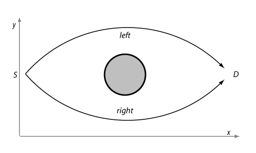
figure-images-xt-ab-0\hyper@anchorend

5.4.1 The Aharonov-Bohm Experiment in Space

In the Aharonov-Bohm experiment ([14]) a particle is sent through a splitter so its wave function is divided in two. One part of the wave function is routed around the left of an ideal solenoid, the other around the right. Outside an ideal solenoid the magnetic field is zero, so the two parts of the wave function see no magnetic field.

They do see a vector potential however. In semi-classical approximation the lowest order phase shift due to the vector potential is given by:

\Hy@raisedlink\hyper@anchorstartequationxtabxtab0\hyper@anchorendieττ′′dτx˙A(x(τ))\Hy@raisedlink\hyper@anchorstart𝑒𝑞𝑢𝑎𝑡𝑖𝑜𝑛𝑥𝑡𝑎𝑏𝑥𝑡𝑎𝑏0\hyper@anchorend𝑖𝑒superscript𝜏superscript𝜏′′d𝜏˙𝑥𝐴𝑥𝜏\Hy@raisedlink{\hyper@anchorstart{equation-xt-ab-xt-ab-0}\hyper@anchorend}ie{\displaystyle\underset{{\tau}^{\prime}}{\overset{{\tau}^{{{}^{\prime\prime}}}}{\int}}\text{d}\tau\dot{\overrightarrow{x}}\cdot\overrightarrow{A}\left(\overrightarrow{x}\left(\tau\right)\right)} (5.182)

It is a function of the magnetic field in the solenoid, but different for the left and right paths.

By changing the magnetic field in the solenoid we can induce a change in the relative phase shift experienced along each path. This in turn includes changes in the interference pattern at the detector.

These have been detected ([871]). Extraordinary.

If the vector potential still has an effect when the magnetic field is zero then the vector potential appears more fundamental than the magnetic field, contrary to all classical thinking.

5.4.2 The Aharonov-Bohm Experiment in Time

As noted, one way to build experimental tests of temporal quantization is to look at "flipped" versions of tests of standard quantum theory, versions with time and a space dimension interchanged.

Flipping time and a space dimension also interchanges the electric and magnetic fields.

Therefore we look a variation on the Aharonov-Bohm experiment where we vary the electric potential in time rather than vary the magnetic potential in space.

Refer to caption
Figure 5.7: Aharonov-Bohm Experiment in Time
\Hy@raisedlink
\hyper@anchorstart

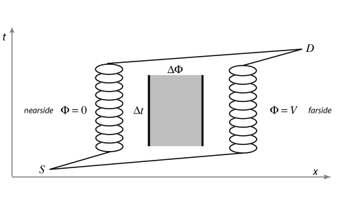
figure-images-xt-ab-1\hyper@anchorend

The setup consists of a splitter, a capacitor we can turn on and off, and a pair of delay loops, one in front of the capacitor, one behind it.

The delay loop has to "park" an electron or other charged particle for a specified (laboratory) time without loss of coherence.

While the capacitor is off we route a particle through the splitter. We send one part of the wave function through a hole in the capacitor, reserving the other part. The near and far sides of the wave function are then fed into delay loops. Then the capacitor is turned on. There is no field outside the capacitor (it is an ideal capacitor) so neither part of the wave function sees a field. However, there is a potential difference between the two sides, so one part sees a potential of V  relative to the other.

Therefore one part of the wave function experiences a phase change given by the integral (per above Constant Potentials):

\Hy@raisedlink\hyper@anchorstartequationxtabxtab1\hyper@anchorendieττ′′dτt˙Φ(x(τ))\Hy@raisedlink\hyper@anchorstart𝑒𝑞𝑢𝑎𝑡𝑖𝑜𝑛𝑥𝑡𝑎𝑏𝑥𝑡𝑎𝑏1\hyper@anchorend𝑖𝑒superscript𝜏superscript𝜏′′d𝜏˙𝑡Φ𝑥𝜏\Hy@raisedlink{\hyper@anchorstart{equation-xt-ab-xt-ab-1}\hyper@anchorend}ie{\displaystyle\underset{{\tau}^{\prime}}{\overset{{\tau}^{{{}^{\prime\prime}}}}{\int}}\text{d}\tau\dot{t}\Phi\left(x\left(\tau\right)\right)} (5.183)

Now the capacitor is turned off and the nearside part of the wave function sent through the hole in the capacitor to be combined with the farside part.

They will interfere destructively or constructively depending on the relative phase change. The relative phase change can be tuned by changing the voltage on the capacitor and the amount of time the capacitor is turned on.

If the potential is V  on the near side and zero on the far side, then the phase shift is:

\Hy@raisedlink\hyper@anchorstartequationxtabxtab2\hyper@anchorendΔϕEmeVΔτ=γeVΔτsimilar-to\Hy@raisedlink\hyper@anchorstart𝑒𝑞𝑢𝑎𝑡𝑖𝑜𝑛𝑥𝑡𝑎𝑏𝑥𝑡𝑎𝑏2\hyper@anchorendΔitalic-ϕ𝐸𝑚𝑒𝑉Δ𝜏𝛾𝑒𝑉Δ𝜏\Hy@raisedlink{\hyper@anchorstart{equation-xt-ab-xt-ab-2}\hyper@anchorend}\Delta\phi\sim-\frac{E}{m}eV\Delta\tau=-\gamma eV\Delta\tau (5.184)

On the farside it is zero.

The interference pattern may therefore be controlled by changing a field after and before the particle passes through the field, with the particle never seeing the field, only the potential $\Phi$.

Discussion

As it happens, we see essentially the same effect in standard quantum theory. The non-relativistic Lagrangian gives:

\Hy@raisedlink\hyper@anchorstartequationxtabxtab3\hyper@anchorendΔϕ¯eVΔτ\Hy@raisedlink\hyper@anchorstart𝑒𝑞𝑢𝑎𝑡𝑖𝑜𝑛𝑥𝑡𝑎𝑏𝑥𝑡𝑎𝑏3\hyper@anchorendΔ¯italic-ϕ𝑒𝑉Δ𝜏\Hy@raisedlink{\hyper@anchorstart{equation-xt-ab-xt-ab-3}\hyper@anchorend}\Delta\overline{\phi}\approx-eV\Delta\tau (5.185)

In the non-relativistic case, the two phase shifts are the same. Therefore the Aharonov-Bohm experiment in time effect is present in standard quantum theory and temporal quantization both.

The original paper by Aharonov and Bohm looked first at the integral over:

\Hy@raisedlink\hyper@anchorstartequationxtabxtab0b\hyper@anchorendieττ′′dτE(x(τ))x˙A(x(τ))\Hy@raisedlink\hyper@anchorstart𝑒𝑞𝑢𝑎𝑡𝑖𝑜𝑛𝑥𝑡𝑎𝑏𝑥𝑡𝑎𝑏0𝑏\hyper@anchorend𝑖𝑒superscript𝜏superscript𝜏′′d𝜏𝐸𝑥𝜏˙𝑥𝐴𝑥𝜏\Hy@raisedlink{\hyper@anchorstart{equation-xt-ab-xt-ab-0b}\hyper@anchorend}-ie{\displaystyle\underset{{\tau}^{\prime}}{\overset{{\tau}^{{{}^{\prime\prime}}}}{\int}}\text{d}\tau E\left(\overrightarrow{x}\left(\tau\right)\right)-\dot{\overrightarrow{x}}\cdot\overrightarrow{A}\left(\overrightarrow{x}\left(\tau\right)\right)} (5.186)

Which includes this contribution from the electric field. Contributions to the Aharonov-Bohm experiment from the electric part have been seen [872].

The novelty is that we are modulating the electric field in time, not just in space, to produce the effect.

Since Aharonov and Rohrlich ([38]) have shown the effect is needed to ensure the self-consistency of quantum mechanics in the case of the vector potential, we expect it is needed to ensure the self-consistency of quantum mechanics in the case of the electric potential as well.

The Aharonov-Bohm experiment in time does not discriminate decisively between temporal quantization and standard quantum theory. But it does suggest that temporal quantization offers a useful way to develop new experiments in time.

5.5 Discussion

\Hy@raisedlink\hyper@anchorstart

xt-disc\hyper@anchorend

A theory is an experiment’s way of creating new experiments.

— Anonymous

Exact Solutions

We have used some fairly rough approximations here.

There is an indirect benefit to use of approximate methods: it avoids excessive dependence on the specifics of temporal quantization, making the predictions if cruder more robust.

With that said, the expressions for the kernel and the Schrödinger equation are exact and in some cases can be solved exactly. Approaches:

  1. 1.

    We can solve the Schrödinger equation directly, posit reasonable initial boundary conditions (i.e. a plane wave to left of the gate, emptiness to its right) and work along the lines developed by Moshinsky ([821], [822]).

  2. 2.

    We can solve for the path integral kernel by using a discrete grid for space and time and discrete steps in laboratory time, then sum over the paths using generating functions and other techniques from discrete analysis, along the lines developed in Feller ([394], [395]) and Graham, Knuth, and Patashnik ([507]).

  3. 3.

    We can model the gates and detector as absorbing walls and apply the methods developed in Marchewka and Schuss ([760], [761]).

Further Experiments

Temporal quantization is an experiment factory.

We have developed just a few experiments here, enough to establish the basic rules, but obviously only a small subset of what is possible.

To date there have been relatively few experiments aimed directly at time: in addition to Lindner’s, we have diffraction in time ([479]) and the delayed choice quantum eraser ([1030], [1032], [688]) as the most obvious.

Further, the most obvious effect of quantum time is to produce increased dispersion in time. It is possible re-mining existing datasets may provide evidence for or against quantum time.

As noted, most foundational experiments can serve as a starting point to develop a test of quantum time; there are potentially hundreds of tests.

We might look at:

  1. 1.

    The Aharonov-Bohm Experiment  (in space) with time-varying solenoid.

  2. 2.

    Tunneling in time: a quantum cat nervous about the occasional appearances of hydrocyanic acid in its chamber might understandably choose to tunnel past the times when the acid is present ([1012]).

  3. 3.

    Gates in energy rather than time.

  4. 4.

    Particle-particle scattering experiments looking for the effects of dispersion in time.

  5. 5.

    Particle-particle scattering experiments taking advantage of the point that if the particle’s wave function is anti-symmetric in time it can have the "wrong" symmetry in space and still satisfy its symmetry requirements.

  6. 6.

    Experiments where we mix rather than flip time and space, as relativistic scattering experiments analyzed from multiple frames.

  7. 7.

    Variations on the Michelson-Morley experiment ([798]). See for instance [220].

  8. 8.

    Apparent violations of dispersion relations. While temporal quantization satisfies unitarity (see Unitarity  above) it does so in four dimensions, not three. This is the sort of thing that will not normally be seen unless explicitly looked for (but see [145], [146], [147], disputed in [1151]).

  9. 9.

    Variations on the experimental designs being used by Hestenes and Catillion to look for Zitterbewegung, used to look for fluctuations in time as well.

  10. 10.

    Variations on electro-magnetically induced transparency (EIT), slow light, the quantum Zeno effect, the quantum eraser, and so on.

To analyze some of these we would have to extend the ideas in this work to the multi-particle case.

Chapter 6 Discussion

\Hy@raisedlink\hyper@anchorstart

disc\hyper@anchorend

The only way of discovering the limits of the possible is to venture a little way past them into the impossible.

— Arthur C. Clarke’s Second Law [263]

Theories need to be pushed as far as they can go before deciding they no longer apply in a given domain.

— Victor Stenger [1075]

Analysis

Our goal has been to quantize time using the rules that we use to quantize space, then see what breaks.

We started with laboratory time $\tau$, time as defined by clocks, laser beams, and graduate students. We posited quantum time $t$, time quantized the same way we quantize space. Laboratory and quantum time represent two ways of looking at same thing: laboratory time or clock time is time as parameter, quantum time is time as observable.

To define what this means in operational terms, we used path integrals (Feynman Path Integrals). We generalized the paths to include motion in time, but made no other changes to the path integrals themselves.

We used Morlet wavelets to analyze the initial wave functions, demonstrate the convergence of the integrals (Convergence), and define a covariant form of the laboratory time (Covariant Definition of Laboratory Time).

The work product of the analysis is the expression for the path integral:

\Hy@raisedlink\hyper@anchorstartequationdisctqfpifinalfullkernel\hyper@anchorendKτ(x′′;x)=limN𝒟xexp(ij=1N+1(m(xjxj1)22ϵ+e(xjxj1)A(xj)+A(xj1)2+m2ϵ))\Hy@raisedlink\hyper@anchorstart𝑒𝑞𝑢𝑎𝑡𝑖𝑜𝑛𝑑𝑖𝑠𝑐𝑡𝑞𝑓𝑝𝑖𝑓𝑖𝑛𝑎𝑙𝑓𝑢𝑙subscript𝑙𝑘𝑒𝑟𝑛𝑒𝑙\hyper@anchorendsubscript𝐾𝜏superscript𝑥′′superscript𝑥𝑁lim𝒟𝑥exp𝑖superscriptsubscript𝑗1𝑁1𝑚superscriptsubscript𝑥𝑗subscript𝑥𝑗122italic-ϵ𝑒subscript𝑥𝑗subscript𝑥𝑗1𝐴subscript𝑥𝑗𝐴subscript𝑥𝑗12𝑚2italic-ϵ\Hy@raisedlink{\hyper@anchorstart{equation-disc-tq-fpi-final-full_{k}ernel}\hyper@anchorend}{K}_{\tau}\left({x}^{{{}^{\prime\prime}}};{x}^{\prime}\right)=\underset{N\rightarrow\infty}{\mathrm{lim}}{\displaystyle\int\mathcal{D}x\mathrm{exp}\left(-i{\displaystyle\sum_{j=1}^{N+1}\left(m\frac{{\left({x}_{j}-{x}_{j-1}\right)}^{2}}{2\epsilon}+e\left({x}_{j}-{x}_{j-1}\right)\frac{A\left({x}_{j}\right)+A\left({x}_{j-1}\right)}{2}+\frac{m}{2}\epsilon\right)}\right)} (6.1)

With measure:

\Hy@raisedlink\hyper@anchorstartequationdisctqfpifinalmeasure\hyper@anchorend𝒟x(im24π2ϵ2)N+1n=1n=Nd4xn\Hy@raisedlink\hyper@anchorstart𝑒𝑞𝑢𝑎𝑡𝑖𝑜𝑛𝑑𝑖𝑠𝑐𝑡𝑞𝑓𝑝𝑖𝑓𝑖𝑛𝑎𝑙𝑚𝑒𝑎𝑠𝑢𝑟𝑒\hyper@anchorend𝒟𝑥superscript𝑖superscript𝑚24superscript𝜋2superscriptitalic-ϵ2𝑁1superscriptsubscriptproduct𝑛1𝑛𝑁superscriptd4subscript𝑥𝑛\Hy@raisedlink{\hyper@anchorstart{equation-disc-tq-fpi-final-measure}\hyper@anchorend}\mathcal{D}x\equiv{\left(-\frac{i{m}^{2}}{4{\pi}^{2}{\epsilon}^{2}}\right)}^{N+1}{\displaystyle\prod_{n=1}^{n=N}{\text{d}}^{\text{4}}{x}_{n}} (6.2)

We used the short time limit of the path integral to derive the Schrödinger equation:

\Hy@raisedlink\hyper@anchorstartequationdisctqseqnderivseqn\hyper@anchorendidψτ(x)dτ=12m((peA)2m2)ψτ(x)\Hy@raisedlink\hyper@anchorstart𝑒𝑞𝑢𝑎𝑡𝑖𝑜𝑛𝑑𝑖𝑠𝑐𝑡𝑞𝑠𝑒𝑞𝑛𝑑𝑒𝑟𝑖𝑣𝑠𝑒𝑞𝑛\hyper@anchorend𝑖𝑑subscript𝜓𝜏𝑥𝑑𝜏12𝑚superscript𝑝𝑒𝐴2superscript𝑚2subscript𝜓𝜏𝑥\Hy@raisedlink{\hyper@anchorstart{equation-disc-tq-seqn-deriv-seqn}\hyper@anchorend}i\frac{d{\psi}_{\tau}\left(x\right)}{d\tau}=-\frac{1}{2m}\left({\left(p-eA\right)}^{2}-{m}^{2}\right){\psi}_{\tau}\left(x\right) (6.3)

Or:

\Hy@raisedlink\hyper@anchorstartequationdisctqseqncoordseqn\hyper@anchorendidψτdτ(t,x)=12m((t+ieΦ(t,x))2(ieA(t,x))2+m2)ψτ(t,x)\Hy@raisedlink\hyper@anchorstart𝑒𝑞𝑢𝑎𝑡𝑖𝑜𝑛𝑑𝑖𝑠𝑐𝑡𝑞𝑠𝑒𝑞𝑛𝑐𝑜𝑜𝑟𝑑𝑠𝑒𝑞𝑛\hyper@anchorend𝑖𝑑subscript𝜓𝜏𝑑𝜏𝑡𝑥12𝑚superscriptsubscript𝑡𝑖𝑒Φ𝑡𝑥2superscript𝑖𝑒𝐴𝑡𝑥2superscript𝑚2subscript𝜓𝜏𝑡𝑥\Hy@raisedlink{\hyper@anchorstart{equation-disc-tq-seqn-coord-seqn}\hyper@anchorend}i\frac{d{\psi}_{\tau}}{d\tau}\left(t,\overrightarrow{x}\right)=\frac{1}{2m}\left({\left({\partial}_{t}+ie\Phi\left(t,\overrightarrow{x}\right)\right)}^{2}-{\left(\overrightarrow{\nabla}-ie\overrightarrow{A}\left(t,\overrightarrow{x}\right)\right)}^{2}+{m}^{2}\right){\psi}_{\tau}\left(t,\overrightarrow{x}\right) (6.4)

We used the Schrödinger equation to demonstrate unitarity (Unitarity)   and analyze the effect of gauge transformations (Gauge Transformations for the Schrödinger Equation).

We derived an operator formalism from the Schrödinger equation (Operators in Time), canonical path integrals from the operator formalism (Canonical Path Integrals), and the original Feynman path integrals from the canonical path integrals (Closing the Circle) – thus closing the circle, and establishing the consistency of all four approaches with each other.

We worked out an invariant definition of the laboratory time (Covariant Definition of Laboratory Time) by breaking the wave function up into its component wavelets and finding an invariant definition of the laboratory time for each.

Slow, Large, and Long Time Limits

We then showed we recover standard quantum theory from temporal quantization in various limits.

  1. 1.

    In the non-relativistic limit (Non-relativistic Limit), we showed we can separate the system into time and space parts, with the space part being the usual standard quantum theory part. In this limit the effect of temporal quantization is to create a kind of temporal fuzz around the baseline standard quantum theory solutions.

  2. 2.

    In the semi-classical limit (Planck’s constant goes to zero), we again got temporal quantization as standard quantum theory plus some fuzz in time (Semi-classical Limit). The expectations are the same for both, but in temporal quantization we see additional dispersion in time. Temporal quantization is to standard quantum theory (with respect to time) as standard quantum theory is to classical mechanics.

  3. 3.

    In the long time limit (Long Time Limit), we got standard quantum theory as the time average of temporal quantization. Over longer periods of time (which might not be that long, anything more than a few hundred attoseconds might do) the stationary states, those with no variation with respect to laboratory time, will dominate. These will be the ones with laboratory energy $\mathscr{E}$  zero:

    \Hy@raisedlink\hyper@anchorstartequationdiscdisc0\hyper@anchorendiddτψτ(t,x)=0Hψτ(t,x)=0=0\Hy@raisedlink\hyper@anchorstart𝑒𝑞𝑢𝑎𝑡𝑖𝑜𝑛𝑑𝑖𝑠𝑐𝑑𝑖𝑠𝑐0\hyper@anchorend𝑖𝑑𝑑𝜏subscript𝜓𝜏𝑡𝑥0𝐻subscript𝜓𝜏𝑡𝑥00\Hy@raisedlink{\hyper@anchorstart{equation-disc-disc-0}\hyper@anchorend}i\frac{d}{d\tau}{\psi}_{\tau}\left(t,\overrightarrow{x}\right)=0\Rightarrow H{\psi}_{\tau}\left(t,\overrightarrow{x}\right)=0\Rightarrow\mathscr{E}=0 (6.5)

    To take advantage of this limit we looked at the cases of non-singular potentials and of bound states:

    1. (a)

      For non-singular potentials (Non-singular Potentials), we reformulated the Schrödinger equation using relative time $\langle{t}_{\tau}\rangle$  and the time gauge:

      \Hy@raisedlink\hyper@anchorstartequationdiscscatterelecttg\hyper@anchorendΛτ(tτ,x)=0tτdtτΦτ(tτ,x)\Hy@raisedlink\hyper@anchorstart𝑒𝑞𝑢𝑎𝑡𝑖𝑜𝑛𝑑𝑖𝑠𝑐𝑠𝑐𝑎𝑡𝑡𝑒𝑟𝑒𝑙𝑒𝑐𝑡𝑡𝑔\hyper@anchorendsubscriptΛ𝜏subscript𝑡𝜏𝑥0subscript𝑡𝜏dsubscriptsuperscript𝑡𝜏subscriptΦ𝜏subscriptsuperscript𝑡𝜏𝑥\Hy@raisedlink{\hyper@anchorstart{equation-disc-scatter-elect-tg}\hyper@anchorend}{\Lambda}_{\tau}\left({t}_{\tau},x\right)={\displaystyle\underset{0}{\overset{{t}_{\tau}}{\int}}\text{d}{{t}^{\prime}}_{\tau}{\Phi}_{\tau}\left({{t}^{\prime}}_{\tau},\overrightarrow{x}\right)} (6.6)

      To expand the Schrödinger equation in powers of the relative time, the difference between quantum and laboratory time.

    2. (b)

      For bound states (Bound States), we used an analysis of the diagonal matrix elements to show that the stationary state condition picks out the usual Bohr orbitals: for each standard quantum theory bound state ${\xi}_{\overline{n}}\left(\overrightarrow{x}\right)$  there is an associated temporal quantization bound state:

      \Hy@raisedlink\hyper@anchorstartequationdiscboundzerolabenergywf\hyper@anchorendψτ(E,n¯)(tτ,x)=12πexp(iEn¯tτ)ξn¯(x)exp(iEn¯τ)\Hy@raisedlink\hyper@anchorstart𝑒𝑞𝑢𝑎𝑡𝑖𝑜𝑛𝑑𝑖𝑠𝑐𝑏𝑜𝑢𝑛𝑑𝑧𝑒𝑟𝑜𝑙𝑎𝑏𝑒𝑛𝑒𝑟𝑔𝑦𝑤𝑓\hyper@anchorendsuperscriptsubscript𝜓𝜏𝐸¯𝑛subscript𝑡𝜏𝑥12𝜋exp𝑖subscript𝐸¯𝑛subscript𝑡𝜏subscript𝜉¯𝑛𝑥exp𝑖subscript𝐸¯𝑛𝜏\Hy@raisedlink{\hyper@anchorstart{equation-disc-bound-zero-labenergy-wf}\hyper@anchorend}{\psi}_{\tau}^{\left(E,\overline{n}\right)}\left({t}_{\tau},\overrightarrow{x}\right)=\frac{1}{\sqrt{2\pi}}\mathrm{exp}\left(-i{E}_{\overline{n}}{t}_{\tau}\right){\xi}_{\overline{n}}\left(\overrightarrow{x}\right)\mathrm{exp}\left(-i{E}_{\overline{n}}\tau\right) (6.7)

      We estimated the dispersion in time (Estimate of Uncertainty in Time) as the same order as the width of the atomic orbitals in space, taking it to under an attosecond in most cases.

Experimental Tests

Having established that temporal quantization looks like standard quantum theory in the slow, large, and long time limits, we turned to asking when would we expect to see effects of fuzzy time? What experimental tests are possible?

We noted that most experiments have two halves, a scatterer and a scatteree. Both have to vary in time or the effects of temporal quantization are likely to average out. This helps explain why quantum time might not have been seen by accident. The most common effect of temporal quantization is additional dispersion in time, easily written off as additional experimental error.

To get a test of quantum time we need to work with time-varying inputs (not steady beams) and work with apparatus that varies in time (choppers, time-varying fields, capacitors that turn on and off, and the like).

We can manufacture tests of quantum time by:

  1. 1.

    Starting with an existing foundational experiment in quantum mechanics then interchanging time and a space dimension.

  2. 2.

    Running a particle with known dispersion in time through an electromagnetic field which is varying rapidly in time.

  3. 3.

    Taking an experiment which implicitly takes a holistic view of time – quantum eraser, Aharonov-Bohm experiment, tests of Aharonov-Bergmann-Lebowitz time-symmetric measurements – and reexamining it from the perspective of quantum time.

We looked at

  1. 1.

    Single and double slit experiments (Slits in Time);

  2. 2.

    Time-varying magnetic fields (Time Dependent Magnetic Field) and electric fields (Time Dependent Electric Field);

  3. 3.

    And a variation on the Aharonov-Bohm experiment (Aharonov-Bohm Experiment).

This is obviously only a small subset of the possible experiments.

Requirements

We therefore argue that temporal quantization satisfies the requirements:

  1. 1.

    Well-defined – with both path integral and Schrödinger equation forms,

  2. 2.

    Manifestly covariant – by construction,

  3. 3.

    Consistent with known experimental results – in the slow, large, and long time limits,

  4. 4.

    Testable – in a large number of ways,

  5. 5.

    And reasonably simple.

The fifth requirement, reasonably simple, is the only one we have not explicitly defended to this point. Arguments in support include:

  1. 1.

    The only change we made to quantize in time was to add motion in time to the usual paths in path integrals. This is the least change we could have made.

  2. 2.

    The demonstration of the convergence of the path integrals is simpler than usual: there are no factors of $i\epsilon$, no artificial Wick rotation, and the like.

  3. 3.

    Unitarity is immediate.

  4. 4.

    By construction, quantum time and the three space coordinates appear in the theory in a fully covariant way 111Recall Weinberg’s observation about the difficulties of demonstrating unitarity and covariance simultaneously.. There is no special role for the quantum time coordinate.

  5. 5.

    The uncertainty principle between quantum time and quantum energy stands on the same basis as the uncertainty principle between space and momentum.

Merits

The principal merit of temporal quantization is that it lets us look at the relationship between time and the quantum in an experimentally testable way.

As noted in the introduction, the possible results are:

  1. 1.

    The behavior of time in quantum mechanics is fully covariant; all quantum effects seen along the space dimensions are seen along the time dimension.

  2. 2.

    We see quantum mechanical effects along the time direction, but they are not fully covariant; the effects along the time direction are less or greater or different than those seen in space.

  3. 3.

    We see no quantum mechanical effects along the time dimension.

In the second and third cases, we might look for associated failures of Lorentz invariance.

In addition, temporal quantization provides a natural starting point for investigation in other areas where time is important, i.e. quantum gravity, quantum computing, and quantum communication.

Further Questions

Areas for further investigation include:

  1. 1.

    Exact solutions for various simple cases.

  2. 2.

    More experimental tests.

  3. 3.

    Further analysis of the semi-classical approximation in temporal quantization.

  4. 4.

    Further clarification of the relationship between the classical, standard quantum theory, and temporal quantization pictures.

  5. 5.

    Extension of temporal quantization to multiple particles.

  6. 6.

    Extension of temporal quantization to statistical mechanics.

  7. 7.

    Implications for the time/energy uncertainty principle.

  8. 8.

    Implications of temporal quantization for the measurement problem.

Appendix A Free Particles

\Hy@raisedlink\hyper@anchorstart

apps\hyper@anchorend

A.1 Overview

\Hy@raisedlink\hyper@anchorstart

free-intro\hyper@anchorend

There is something fascinating about science. One gets such wholesale returns of conjecture out of such a trifling investment of fact.

— Mark Twain [1139]

We assemble some useful properties of the free particle wave functions and kernels here. We look at:

  1. 1.

    The Time/Space Representation,

  2. 2.

    The Energy/Momentum Representation,

  3. 3.

    And the Time/Momentum Representation.

A.2 Time/Space Representation

\Hy@raisedlink\hyper@anchorstart

free-fourt\hyper@anchorend

We look at the block time case then the relative time case.

A.2.1 In Block Time

We look at the kernel, then apply it to plane waves and Gaussian test functions.

Kernel

The free kernel may be written as a product of time and space parts:

\Hy@raisedlink\hyper@anchorstartequationfreefourtfreekernelkprodt\hyper@anchorendKτ(x′′;x)=Kτ(t′′;t)K¯τ(x′′;x)\Hy@raisedlink{\hyper@anchorstart{equation-free-fourt-free-kernel-kprodt}\hyper@anchorend}{K}_{\tau}\left({x}^{{{}^{\prime\prime}}};{x}^{\prime}\right)={\stackrel{{\scriptstyle\frown}}{{K}}}_{\tau}\left({t}^{{{}^{\prime\prime}}};{t}^{\prime}\right){\overline{K}}_{\tau}\left(\overrightarrow{{x}^{{{}^{\prime\prime}}}};\overrightarrow{{x}^{\prime}}\right) (A.1)

Time part:

\Hy@raisedlink\hyper@anchorstartequationfreefourtfreeonetkernel\hyper@anchorendKτ(t′′;t)=im2πτexp(im(t′′t)22τimτ2)subscriptsuperscript𝐾𝜏\Hy@raisedlink\hyper@anchorstart𝑒𝑞𝑢𝑎𝑡𝑖𝑜𝑛𝑓𝑟𝑒𝑒𝑓𝑜𝑢𝑟𝑡𝑓𝑟𝑒𝑒𝑜𝑛𝑒𝑡𝑘𝑒𝑟𝑛𝑒𝑙\hyper@anchorendsuperscript𝑡′′superscript𝑡𝑖𝑚2𝜋𝜏exp𝑖𝑚superscriptsuperscript𝑡′′superscript𝑡22𝜏𝑖𝑚𝜏2\Hy@raisedlink{\hyper@anchorstart{equation-free-fourt-free-onet-kernel}\hyper@anchorend}{\stackrel{{\scriptstyle\frown}}{{K}}}_{\tau}\left({t}^{{{}^{\prime\prime}}};{t}^{\prime}\right)=\sqrt{\frac{im}{2\pi\tau}}\mathrm{exp}\left(-im\frac{{\left({t}^{{{}^{\prime\prime}}}-{t}^{\prime}\right)}^{2}}{2\tau}-im\frac{\tau}{2}\right) (A.2)

Space part:

\Hy@raisedlink\hyper@anchorstartequationfreefourtfreefourtkernel3\hyper@anchorendK¯τ(x′′;x)=m2πiτ3exp(im2τ(x′′x)2)\Hy@raisedlink\hyper@anchorstart𝑒𝑞𝑢𝑎𝑡𝑖𝑜𝑛𝑓𝑟𝑒𝑒𝑓𝑜𝑢𝑟𝑡𝑓𝑟𝑒𝑒𝑓𝑜𝑢𝑟𝑡𝑘𝑒𝑟𝑛𝑒𝑙3\hyper@anchorendsubscript¯𝐾𝜏superscript𝑥′′superscript𝑥superscript𝑚2𝜋𝑖𝜏3exp𝑖𝑚2𝜏superscriptsuperscript𝑥′′superscript𝑥2\Hy@raisedlink{\hyper@anchorstart{equation-free-fourt-free-fourt-kernel3}\hyper@anchorend}{\overline{K}}_{\tau}\left(\overrightarrow{{x}^{{{}^{\prime\prime}}}};\overrightarrow{{x}^{\prime}}\right)={\sqrt{\frac{m}{2\pi i\tau}}}^{3}\mathrm{exp}\left(\frac{im}{2\tau}{\left(\overrightarrow{{x}^{{{}^{\prime\prime}}}}-\overrightarrow{{x}^{\prime}}\right)}^{2}\right) (A.3)
Plane Waves

We take the initial plane wave as:

\Hy@raisedlink\hyper@anchorstartequationfreefourtfreeplanet0\hyper@anchorendϕ0(x)=14π2exp(ipx)\Hy@raisedlink\hyper@anchorstart𝑒𝑞𝑢𝑎𝑡𝑖𝑜𝑛𝑓𝑟𝑒𝑒𝑓𝑜𝑢𝑟𝑡𝑓𝑟𝑒𝑒𝑝𝑙𝑎𝑛𝑒𝑡0\hyper@anchorendsubscriptitalic-ϕ0𝑥14superscript𝜋2exp𝑖𝑝𝑥\Hy@raisedlink{\hyper@anchorstart{equation-free-fourt-free-planet-0}\hyper@anchorend}{\phi}_{0}\left(x\right)=\frac{1}{4{\pi}^{2}}\mathrm{exp}\left(-ipx\right) (A.4)

By applying the kernel we get the dependence on laboratory time:

\Hy@raisedlink\hyper@anchorstartequationfreefourtfreeplanet3\hyper@anchorendϕτ(x)=14π2exp(ipxipτ)\Hy@raisedlink\hyper@anchorstart𝑒𝑞𝑢𝑎𝑡𝑖𝑜𝑛𝑓𝑟𝑒𝑒𝑓𝑜𝑢𝑟𝑡𝑓𝑟𝑒𝑒𝑝𝑙𝑎𝑛𝑒𝑡3\hyper@anchorendsubscriptitalic-ϕ𝜏𝑥14superscript𝜋2exp𝑖𝑝𝑥𝑖subscript𝑝𝜏\Hy@raisedlink{\hyper@anchorstart{equation-free-fourt-free-planet-3}\hyper@anchorend}{\phi}_{\tau}\left(x\right)=\frac{1}{4{\pi}^{2}}\mathrm{exp}\left(-ipx-i{\mathscr{E}}_{p}\tau\right) (A.5)

With the laboratory energy ${\mathscr{E}}_{p}$:

\Hy@raisedlink\hyper@anchorstartequationfreefourtfreeplanet2\hyper@anchorendpE2p2m22m\Hy@raisedlink\hyper@anchorstart𝑒𝑞𝑢𝑎𝑡𝑖𝑜𝑛𝑓𝑟𝑒𝑒𝑓𝑜𝑢𝑟𝑡𝑓𝑟𝑒𝑒𝑝𝑙𝑎𝑛𝑒𝑡2\hyper@anchorendsubscript𝑝superscript𝐸2superscript𝑝2superscript𝑚22𝑚\Hy@raisedlink{\hyper@anchorstart{equation-free-fourt-free-planet-2}\hyper@anchorend}{\mathscr{E}}_{p}\equiv-\frac{{E}^{2}-{\overrightarrow{p}}^{2}-{m}^{2}}{2m} (A.6)

The ${\phi}_{\tau}\left(x\right)$  are eigenstates of the free Hamiltonian with eigenvalues ${\mathscr{E}}_{p}$:

\Hy@raisedlink\hyper@anchorstartequationfreefourtfreeplanet1\hyper@anchorendH(free)ϕτ(x)=pϕτ(x),H(free)=12m(t22+m2)formulae-sequence\Hy@raisedlink\hyper@anchorstart𝑒𝑞𝑢𝑎𝑡𝑖𝑜𝑛𝑓𝑟𝑒𝑒𝑓𝑜𝑢𝑟𝑡𝑓𝑟𝑒𝑒𝑝𝑙𝑎𝑛𝑒𝑡1\hyper@anchorendsuperscript𝐻𝑓𝑟𝑒𝑒subscriptitalic-ϕ𝜏𝑥subscript𝑝subscriptitalic-ϕ𝜏𝑥superscript𝐻𝑓𝑟𝑒𝑒12𝑚superscriptsubscript𝑡2superscript2superscript𝑚2\Hy@raisedlink{\hyper@anchorstart{equation-free-fourt-free-planet-1}\hyper@anchorend}{H}^{\left(free\right)}{\phi}_{\tau}\left(x\right)={\mathscr{E}}_{p}{\phi}_{\tau}\left(x\right),{H}^{\left(free\right)}=\frac{1}{2m}\left({\partial}_{t}^{2}-{\nabla}^{2}+{m}^{2}\right) (A.7)

The stationary states are onshell:

\Hy@raisedlink\hyper@anchorstartequationfreefourtfreeplanet3d\hyper@anchorendiddτϕτ(x)=0p=0E=E¯p\Hy@raisedlink\hyper@anchorstart𝑒𝑞𝑢𝑎𝑡𝑖𝑜𝑛𝑓𝑟𝑒𝑒𝑓𝑜𝑢𝑟𝑡𝑓𝑟𝑒𝑒𝑝𝑙𝑎𝑛𝑒𝑡3𝑑\hyper@anchorend𝑖𝑑𝑑𝜏subscriptitalic-ϕ𝜏𝑥0subscript𝑝0𝐸subscript¯𝐸𝑝\Hy@raisedlink{\hyper@anchorstart{equation-free-fourt-free-planet-3d}\hyper@anchorend}i\frac{d}{d\tau}{\phi}_{\tau}\left(x\right)=0\rightarrow{\mathscr{E}}_{p}=0\rightarrow E={\overline{E}}_{\overrightarrow{p}} (A.8)

With the onshell energy defined as:

\Hy@raisedlink\hyper@anchorstartequationfreefourtfreeplanet3c\hyper@anchorendE¯pp2+m2\Hy@raisedlink\hyper@anchorstart𝑒𝑞𝑢𝑎𝑡𝑖𝑜𝑛𝑓𝑟𝑒𝑒𝑓𝑜𝑢𝑟𝑡𝑓𝑟𝑒𝑒𝑝𝑙𝑎𝑛𝑒𝑡3𝑐\hyper@anchorendsubscript¯𝐸𝑝superscript𝑝2superscript𝑚2\Hy@raisedlink{\hyper@anchorstart{equation-free-fourt-free-planet-3c}\hyper@anchorend}{\overline{E}}_{\overrightarrow{p}}\equiv\sqrt{{\overrightarrow{p}}^{2}+{m}^{2}} (A.9)

Therefore the stationary states are given by:

\Hy@raisedlink\hyper@anchorstartequationfreefourtfreeplanet3b\hyper@anchorendϕτ(onshell)(x)=14π2exp(iE¯pt+ipx)\Hy@raisedlink\hyper@anchorstart𝑒𝑞𝑢𝑎𝑡𝑖𝑜𝑛𝑓𝑟𝑒𝑒𝑓𝑜𝑢𝑟𝑡𝑓𝑟𝑒𝑒𝑝𝑙𝑎𝑛𝑒𝑡3𝑏\hyper@anchorendsuperscriptsubscriptitalic-ϕ𝜏𝑜𝑛𝑠𝑒𝑙𝑙𝑥14superscript𝜋2exp𝑖subscript¯𝐸𝑝𝑡𝑖𝑝𝑥\Hy@raisedlink{\hyper@anchorstart{equation-free-fourt-free-planet-3b}\hyper@anchorend}{\phi}_{\tau}^{\left(onshell\right)}\left(x\right)=\frac{1}{4{\pi}^{2}}\mathrm{exp}\left(-i{\overline{E}}_{\overrightarrow{p}}t+i\overrightarrow{p}\cdot\overrightarrow{x}\right) (A.10)
Gaussian Test Functions

We take the initial Gaussian test function as:

\Hy@raisedlink\hyper@anchorstartequationfreefourtfreefourtphi0\hyper@anchorendψ0(x)=1π4det(Σ0)4exp(ipμ(0)xμ12Σ0μν(xμx¯0μ)(xnx¯0ν))\Hy@raisedlink\hyper@anchorstart𝑒𝑞𝑢𝑎𝑡𝑖𝑜𝑛𝑓𝑟𝑒𝑒𝑓𝑜𝑢𝑟𝑡𝑓𝑟𝑒𝑒𝑓𝑜𝑢𝑟𝑡𝑝𝑖0\hyper@anchorendsubscript𝜓0𝑥41superscript𝜋4detsubscriptΣ0exp𝑖superscriptsubscript𝑝𝜇0superscript𝑥𝜇12superscriptsubscriptΣ0𝜇𝜈superscript𝑥𝜇superscriptsubscript¯𝑥0𝜇superscript𝑥𝑛superscriptsubscript¯𝑥0𝜈\Hy@raisedlink{\hyper@anchorstart{equation-free-fourt-free-fourt-phi0}\hyper@anchorend}{\psi}_{0}\left(x\right)=\sqrt[4]{\frac{1}{{\pi}^{4}\mathrm{det}\left({\Sigma}_{0}\right)}}\mathrm{exp}\left(-i{p}_{\mu}^{\left(0\right)}{x}^{\mu}-\frac{1}{2{\Sigma}_{0}^{\mu\nu}}\left({x}^{\mu}-{\overline{x}}_{0}^{\mu}\right)\left({x}^{n}-{\overline{x}}_{0}^{\nu}\right)\right) (A.11)

With the dispersion matrix $\Sigma$  diagonal:

\Hy@raisedlink\hyper@anchorstartequationfreefourtfreefourtsigma0\hyper@anchorendΣ0μν=(σ020000σ120000σ220000σ32)\Hy@raisedlink\hyper@anchorstart𝑒𝑞𝑢𝑎𝑡𝑖𝑜𝑛𝑓𝑟𝑒𝑒𝑓𝑜𝑢𝑟𝑡𝑓𝑟𝑒𝑒𝑓𝑜𝑢𝑟𝑡𝑠𝑖𝑔𝑚𝑎0\hyper@anchorendsuperscriptsubscriptΣ0𝜇𝜈superscriptsubscript𝜎020000superscriptsubscript𝜎120000superscriptsubscript𝜎220000superscriptsubscript𝜎32\Hy@raisedlink{\hyper@anchorstart{equation-free-fourt-free-fourt-sigma0}\hyper@anchorend}{\Sigma}_{0}^{\mu\nu}=\left(\begin{array}[]{cccc}{\sigma}_{0}^{2}&0&0&0\\ 0&{\sigma}_{1}^{2}&0&0\\ 0&0&{\sigma}_{2}^{2}&0\\ 0&0&0&{\sigma}_{3}^{2}\end{array}\right) (A.12)

By applying the kernel we get the dependence on laboratory time:

\Hy@raisedlink\hyper@anchorstartequationfreefourtfreefourtphitau\hyper@anchorendψτ(x)=det(Σ0μν)π441det(Στμν)exp(ip0μxμ12Στμν(xμx¯τμ)(xνx¯τν)+ip02m22mτ)\Hy@raisedlink\hyper@anchorstart𝑒𝑞𝑢𝑎𝑡𝑖𝑜𝑛𝑓𝑟𝑒𝑒𝑓𝑜𝑢𝑟𝑡𝑓𝑟𝑒𝑒𝑓𝑜𝑢𝑟𝑡𝑝𝑖𝑡𝑎𝑢\hyper@anchorendsubscript𝜓𝜏𝑥4detsuperscriptsubscriptΣ0𝜇𝜈superscript𝜋41detsuperscriptsubscriptΣ𝜏𝜇𝜈exp𝑖superscriptsubscript𝑝0𝜇subscript𝑥𝜇12superscriptsubscriptΣ𝜏𝜇𝜈superscript𝑥𝜇superscriptsubscript¯𝑥𝜏𝜇superscript𝑥𝜈superscriptsubscript¯𝑥𝜏𝜈𝑖superscriptsubscript𝑝02superscript𝑚22𝑚𝜏\Hy@raisedlink{\hyper@anchorstart{equation-free-fourt-free-fourt-phitau}\hyper@anchorend}{\psi}_{\tau}\left(x\right)=\sqrt[4]{\frac{\mathrm{det}\left({\Sigma}_{0}^{\mu\nu}\right)}{{\pi}^{4}}}\sqrt{\frac{1}{\mathrm{det}\left({\Sigma}_{\tau}^{\mu\nu}\right)}}\mathrm{exp}\left(-i{p}_{0}^{\mu}{x}_{\mu}-\frac{1}{2{\Sigma}_{\tau}^{\mu\nu}}\left({x}^{\mu}-{\overline{x}}_{\tau}^{\mu}\right)\left({x}^{\nu}-{\overline{x}}_{\tau}^{\nu}\right)+i\frac{{p}_{0}^{2}-{m}^{2}}{2m}\tau\right) (A.13)

The expectations of coordinates evolve with laboratory time:

\Hy@raisedlink\hyper@anchorstartequationfreefourtfreefourtaverage\hyper@anchorendx¯τμxμτ=x¯0μ+p0μmτ\Hy@raisedlink\hyper@anchorstart𝑒𝑞𝑢𝑎𝑡𝑖𝑜𝑛𝑓𝑟𝑒𝑒𝑓𝑜𝑢𝑟𝑡𝑓𝑟𝑒𝑒𝑓𝑜𝑢𝑟𝑡𝑎𝑣𝑒𝑟𝑎𝑔𝑒\hyper@anchorendsuperscriptsubscript¯𝑥𝜏𝜇subscriptdelimited-⟨⟩superscript𝑥𝜇𝜏superscriptsubscript¯𝑥0𝜇superscriptsubscript𝑝0𝜇𝑚𝜏\Hy@raisedlink{\hyper@anchorstart{equation-free-fourt-free-fourt-average}\hyper@anchorend}{\overline{x}}_{\tau}^{\mu}\equiv{\langle{x}^{\mu}\rangle}_{\tau}={\overline{x}}_{0}^{\mu}+\frac{{p}_{0}^{\mu}}{m}\tau (A.14)

As does the dispersion matrix:

\Hy@raisedlink\hyper@anchorstartequationfreefourtfreefourtsigmatau\hyper@anchorendΣτμν=(σ02iτm0000σ12+iτm0000σ22+iτm0000σ32+iτm)=(σ02fτ(0)0000σ12fτ(1)0000σ22fτ(2)0000σ32fτ(3))\Hy@raisedlink\hyper@anchorstart𝑒𝑞𝑢𝑎𝑡𝑖𝑜𝑛𝑓𝑟𝑒𝑒𝑓𝑜𝑢𝑟𝑡𝑓𝑟𝑒𝑒𝑓𝑜𝑢𝑟𝑡𝑠𝑖𝑔𝑚𝑎𝑡𝑎𝑢\hyper@anchorendsuperscriptsubscriptΣ𝜏𝜇𝜈superscriptsubscript𝜎02𝑖𝜏𝑚0000superscriptsubscript𝜎12𝑖𝜏𝑚0000superscriptsubscript𝜎22𝑖𝜏𝑚0000superscriptsubscript𝜎32𝑖𝜏𝑚superscriptsubscript𝜎02superscriptsubscript𝑓𝜏00000superscriptsubscript𝜎12superscriptsubscript𝑓𝜏10000superscriptsubscript𝜎22superscriptsubscript𝑓𝜏20000superscriptsubscript𝜎32superscriptsubscript𝑓𝜏3\Hy@raisedlink{\hyper@anchorstart{equation-free-fourt-free-fourt-sigmatau}\hyper@anchorend}{\Sigma}_{\tau}^{\mu\nu}=\left(\begin{array}[]{cccc}{\sigma}_{0}^{2}-i\frac{\tau}{m}&0&0&0\\ 0&{\sigma}_{1}^{2}+i\frac{\tau}{m}&0&0\\ 0&0&{\sigma}_{2}^{2}+i\frac{\tau}{m}&0\\ 0&0&0&{\sigma}_{3}^{2}+i\frac{\tau}{m}\end{array}\right)=\left(\begin{array}[]{cccc}{\sigma}_{0}^{2}{f}_{\tau}^{\left(0\right)}&0&0&0\\ 0&{\sigma}_{1}^{2}{f}_{\tau}^{\left(1\right)}&0&0\\ 0&0&{\sigma}_{2}^{2}{f}_{\tau}^{\left(2\right)}&0\\ 0&0&0&{\sigma}_{3}^{2}{f}_{\tau}^{\left(3\right)}\end{array}\right) (A.15)

$\psi$  is not an eigenstate of the free Hamiltonian but it does satisfy the free Schrödinger equation:

\Hy@raisedlink\hyper@anchorstartequationfreefourtfreeseqn0\hyper@anchorendiψτ(x)τ=12m(2t22+m2)ψτ(x)\Hy@raisedlink\hyper@anchorstart𝑒𝑞𝑢𝑎𝑡𝑖𝑜𝑛𝑓𝑟𝑒𝑒𝑓𝑜𝑢𝑟𝑡𝑓𝑟𝑒𝑒𝑠𝑒𝑞𝑛0\hyper@anchorend𝑖subscript𝜓𝜏𝑥𝜏12𝑚superscript2superscript𝑡2superscript2superscript𝑚2subscript𝜓𝜏𝑥\Hy@raisedlink{\hyper@anchorstart{equation-free-fourt-free-seqn-0}\hyper@anchorend}i\frac{\partial{\psi}_{\tau}\left(x\right)}{\partial\tau}=\frac{1}{2m}\left(\frac{{\partial}^{2}}{\partial{t}^{2}}-{\nabla}^{2}+{m}^{2}\right){\psi}_{\tau}\left(x\right) (A.16)

With probability density:

\Hy@raisedlink\hyper@anchorstartequationfreefourtfreefourtrho\hyper@anchorendρτ(x)=1π4μ=03σμ2(1+τ2m2σμ4)exp(μ=03(xμ(x¯0μ+p0μmτ))2σμ2(1+τ2m2σμ4))\Hy@raisedlink\hyper@anchorstart𝑒𝑞𝑢𝑎𝑡𝑖𝑜𝑛𝑓𝑟𝑒𝑒𝑓𝑜𝑢𝑟𝑡𝑓𝑟𝑒𝑒𝑓𝑜𝑢𝑟𝑡𝑟𝑜\hyper@anchorendsubscript𝜌𝜏𝑥1superscript𝜋4superscriptsubscriptproduct𝜇03superscriptsubscript𝜎𝜇21superscript𝜏2superscript𝑚2superscriptsubscript𝜎𝜇4expsuperscriptsubscript𝜇03superscriptsuperscript𝑥𝜇superscriptsubscript¯𝑥0𝜇superscriptsubscript𝑝0𝜇𝑚𝜏2superscriptsubscript𝜎𝜇21superscript𝜏2superscript𝑚2superscriptsubscript𝜎𝜇4\Hy@raisedlink{\hyper@anchorstart{equation-free-fourt-free-fourt-rho}\hyper@anchorend}{\rho}_{\tau}\left(x\right)=\sqrt{\frac{1}{{\pi}^{4}{\displaystyle\prod_{\mu=0}^{3}{\sigma}_{\mu}^{2}\left(1+\frac{{\tau}^{2}}{{m}^{2}{\sigma}_{\mu}^{4}}\right)}}}\mathrm{exp}\left(-{\displaystyle\sum_{\mu=0}^{3}\frac{{\left({x}^{\mu}-\left({\overline{x}}_{0}^{\mu}+\frac{{p}_{0}^{\mu}}{m}\tau\right)\right)}^{2}}{{\sigma}_{\mu}^{2}\left(1+\frac{{\tau}^{2}}{{m}^{2}{\sigma}_{\mu}^{4}}\right)}}\right) (A.17)

And uncertainties:

\Hy@raisedlink\hyper@anchorstartequationfreefourtfreefourtdispersions\hyper@anchorend(xμx¯τμ)2=σμ22|1+τ2m2σμ4|\Hy@raisedlink\hyper@anchorstart𝑒𝑞𝑢𝑎𝑡𝑖𝑜𝑛𝑓𝑟𝑒𝑒𝑓𝑜𝑢𝑟𝑡𝑓𝑟𝑒𝑒𝑓𝑜𝑢𝑟𝑡𝑑𝑖𝑠𝑝𝑒𝑟𝑠𝑖𝑜𝑛𝑠\hyper@anchorenddelimited-⟨⟩superscriptsuperscript𝑥𝜇superscriptsubscript¯𝑥𝜏𝜇2superscriptsubscript𝜎𝜇221superscript𝜏2superscript𝑚2superscriptsubscript𝜎𝜇4\Hy@raisedlink{\hyper@anchorstart{equation-free-fourt-free-fourt-dispersions}\hyper@anchorend}\langle{\left({x}^{\mu}-{\overline{x}}_{\tau}^{\mu}\right)}^{2}\rangle=\frac{{\sigma}_{\mu}^{2}}{2}\left|1+\frac{{\tau}^{2}}{{m}^{2}{\sigma}_{\mu}^{4}}\right| (A.18)

$\psi$  has a natural decomposition into time and space parts:

\Hy@raisedlink\hyper@anchorstartequationfreefourtfreefourtdecomp\hyper@anchorendψτ(t,x)=χτ(t)ξτ(x)\Hy@raisedlink\hyper@anchorstart𝑒𝑞𝑢𝑎𝑡𝑖𝑜𝑛𝑓𝑟𝑒𝑒𝑓𝑜𝑢𝑟𝑡𝑓𝑟𝑒𝑒𝑓𝑜𝑢𝑟𝑡𝑑𝑒𝑐𝑜𝑚𝑝\hyper@anchorendsubscript𝜓𝜏𝑡𝑥subscript𝜒𝜏𝑡subscript𝜉𝜏𝑥\Hy@raisedlink{\hyper@anchorstart{equation-free-fourt-free-fourt-decomp}\hyper@anchorend}{\psi}_{\tau}\left(t,x\right)={\chi}_{\tau}\left(t\right){\xi}_{\tau}\left(\overrightarrow{x}\right) (A.19)

Time part:

\Hy@raisedlink\hyper@anchorstartequationfreefourtfreeonetchitq\hyper@anchorendχτ(t)=1πσ0241fτ(0)exp(iE0t12σ02fτ(0)(tt¯τ)2+iE02m22mτ)\Hy@raisedlink\hyper@anchorstart𝑒𝑞𝑢𝑎𝑡𝑖𝑜𝑛𝑓𝑟𝑒𝑒𝑓𝑜𝑢𝑟𝑡𝑓𝑟𝑒𝑒𝑜𝑛𝑒𝑡𝑐𝑖𝑡𝑞\hyper@anchorendsubscript𝜒𝜏𝑡41𝜋superscriptsubscript𝜎021superscriptsubscript𝑓𝜏0exp𝑖subscript𝐸0𝑡12superscriptsubscript𝜎02superscriptsubscript𝑓𝜏0superscript𝑡subscript¯𝑡𝜏2𝑖superscriptsubscript𝐸02superscript𝑚22𝑚𝜏\Hy@raisedlink{\hyper@anchorstart{equation-free-fourt-free-onet-chitq}\hyper@anchorend}{\chi}_{\tau}\left(t\right)=\sqrt[4]{\frac{1}{\pi{\sigma}_{0}^{2}}}\sqrt{\frac{1}{{f}_{\tau}^{\left(0\right)}}}\mathrm{exp}\left(-i{E}_{0}t-\frac{1}{2{\sigma}_{0}^{2}{f}_{\tau}^{\left(0\right)}}{\left(t-{\overline{t}}_{\tau}\right)}^{2}+i\frac{{E}_{0}^{2}-{m}^{2}}{2m}\tau\right) (A.20)

The space part is the standard quantum theory wave function:

\Hy@raisedlink\hyper@anchorstartequationfreefourtfreethreetxitau\hyper@anchorendξτ(x)=1π3det(Στ)4exp(ip0x(xx¯τ)12Στ(xx¯τ)ip022mτ)\Hy@raisedlink\hyper@anchorstart𝑒𝑞𝑢𝑎𝑡𝑖𝑜𝑛𝑓𝑟𝑒𝑒𝑓𝑜𝑢𝑟𝑡𝑓𝑟𝑒𝑒𝑡𝑟𝑒𝑒𝑡𝑥𝑖𝑡𝑎𝑢\hyper@anchorendsubscript𝜉𝜏𝑥41superscript𝜋3detsubscriptΣ𝜏exp𝑖subscript𝑝0𝑥𝑥subscript¯𝑥𝜏12subscriptΣ𝜏𝑥subscript¯𝑥𝜏𝑖superscriptsubscript𝑝022𝑚𝜏\Hy@raisedlink{\hyper@anchorstart{equation-free-fourt-free-threet-xitau}\hyper@anchorend}{\xi}_{\tau}\left(\overrightarrow{x}\right)=\sqrt[4]{\frac{1}{{\pi}^{3}\mathrm{det}\left({\overleftrightarrow{\Sigma}}_{\tau}\right)}}\mathrm{exp}\left(i{\overrightarrow{p}}_{0}\cdot\overrightarrow{x}-\left(\overrightarrow{x}-{\overline{x}}_{\tau}\right)\cdot\frac{1}{2{\overleftrightarrow{\Sigma}}_{\tau}}\cdot\left(\overrightarrow{x}-{\overline{x}}_{\tau}\right)-i\frac{{\overrightarrow{p}}_{0}^{2}}{2m}\tau\right) (A.21)

A.2.2 In Relative Time

Recall that the relative time is defined as the difference between the absolute quantum time and the laboratory time ${t}_{\tau}\equiv t-\tau$. We look at the relative time kernel, then apply it to plane waves and Gaussian test functions.

Kernel

Only the time part of the kernel is affected by a switch from block time to relative time:

\Hy@raisedlink\hyper@anchorstartequationfreefourtfreereltimetkernel\hyper@anchorendKτ(rel)(t′′τ;t0)=im2πτexp(im(t′′τt0+τ)22τimτ2)superscriptsubscriptsuperscript𝐾𝜏𝑟𝑒𝑙\Hy@raisedlink\hyper@anchorstart𝑒𝑞𝑢𝑎𝑡𝑖𝑜𝑛𝑓𝑟𝑒𝑒𝑓𝑜𝑢𝑟𝑡𝑓𝑟𝑒𝑒𝑟𝑒𝑙𝑡𝑖𝑚𝑒𝑡𝑘𝑒𝑟𝑛𝑒𝑙\hyper@anchorendsubscriptsuperscript𝑡′′𝜏subscriptsuperscript𝑡0𝑖𝑚2𝜋𝜏exp𝑖𝑚superscriptsubscriptsuperscript𝑡′′𝜏subscriptsuperscript𝑡0𝜏22𝜏𝑖𝑚𝜏2\Hy@raisedlink{\hyper@anchorstart{equation-free-fourt-free-reltimet-kernel}\hyper@anchorend}{\stackrel{{\scriptstyle\frown}}{{K}}}_{\tau}^{\left(rel\right)}\left({{t}^{{{}^{\prime\prime}}}}_{\tau};{{t}^{\prime}}_{0}\right)=\sqrt{\frac{im}{2\pi\tau}}\mathrm{exp}\left(-im\frac{{\left({{t}^{{{}^{\prime\prime}}}}_{\tau}-{{t}^{\prime}}_{0}+\tau\right)}^{2}}{2\tau}-im\frac{\tau}{2}\right) (A.22)

Or:

\Hy@raisedlink\hyper@anchorstartequationfreefourtfreereltimetkernel2\hyper@anchorendKτ(rel)(t′′τ;t0)=im2πτexp(im(t′′τt0)22τim(t′′τt0+τ))superscriptsubscriptsuperscript𝐾𝜏𝑟𝑒𝑙\Hy@raisedlink\hyper@anchorstart𝑒𝑞𝑢𝑎𝑡𝑖𝑜𝑛𝑓𝑟𝑒𝑒𝑓𝑜𝑢𝑟𝑡𝑓𝑟𝑒𝑒𝑟𝑒𝑙𝑡𝑖𝑚𝑒𝑡𝑘𝑒𝑟𝑛𝑒𝑙2\hyper@anchorendsubscriptsuperscript𝑡′′𝜏subscriptsuperscript𝑡0𝑖𝑚2𝜋𝜏exp𝑖𝑚superscriptsubscriptsuperscript𝑡′′𝜏subscriptsuperscript𝑡022𝜏𝑖𝑚subscriptsuperscript𝑡′′𝜏subscriptsuperscript𝑡0𝜏\Hy@raisedlink{\hyper@anchorstart{equation-free-fourt-free-reltimet-kernel2}\hyper@anchorend}{\stackrel{{\scriptstyle\frown}}{{K}}}_{\tau}^{\left(rel\right)}\left({{t}^{{{}^{\prime\prime}}}}_{\tau};{{t}^{\prime}}_{0}\right)=\sqrt{\frac{im}{2\pi\tau}}\mathrm{exp}\left(-im\frac{{\left({{t}^{{{}^{\prime\prime}}}}_{\tau}-{{t}^{\prime}}_{0}\right)}^{2}}{2\tau}-im\left({{t}^{{{}^{\prime\prime}}}}_{\tau}-{{t}^{\prime}}_{0}+\tau\right)\right) (A.23)
Plane Waves

The relative time plane wave is:

\Hy@raisedlink\hyper@anchorstartequationfreefourtfreeplanet7\hyper@anchorendϕτ(rel)(x)=14π2exp(iEtτ+ipxi(p+E)τ)\Hy@raisedlink\hyper@anchorstart𝑒𝑞𝑢𝑎𝑡𝑖𝑜𝑛𝑓𝑟𝑒𝑒𝑓𝑜𝑢𝑟𝑡𝑓𝑟𝑒𝑒𝑝𝑙𝑎𝑛𝑒𝑡7\hyper@anchorendsuperscriptsubscriptitalic-ϕ𝜏𝑟𝑒𝑙𝑥14superscript𝜋2exp𝑖𝐸subscript𝑡𝜏𝑖𝑝𝑥𝑖subscript𝑝𝐸𝜏\Hy@raisedlink{\hyper@anchorstart{equation-free-fourt-free-planet-7}\hyper@anchorend}{\phi}_{\tau}^{\left(rel\right)}\left(x\right)=\frac{1}{4{\pi}^{2}}\mathrm{exp}\left(-iE{t}_{\tau}+i\overrightarrow{p}\cdot\overrightarrow{x}-i\left({\mathscr{E}}_{p}+E\right)\tau\right) (A.24)

We break out the quantum energy $E$  into space and time parts:

\Hy@raisedlink\hyper@anchorstartequationfreefourtfreeplanet8\hyper@anchorendE=E¯p+Ep,EpEE¯p\Hy@raisedlink{\hyper@anchorstart{equation-free-fourt-free-planet-8}\hyper@anchorend}E={\overline{E}}_{\overrightarrow{p}}+{\stackrel{{\scriptstyle\frown}}{{E}}}_{p},{\stackrel{{\scriptstyle\frown}}{{E}}}_{p}\equiv E-{\overline{E}}_{\overrightarrow{p}} (A.25)

The relative time laboratory energy is:

\Hy@raisedlink\hyper@anchorstartequationfreefourtfreeplanet9\hyper@anchorendp(rel)=E¯p+p(rel),p(rel)(γp1)EpEp22m,γp11v2=E¯pm\Hy@raisedlink{\hyper@anchorstart{equation-free-fourt-free-planet-9}\hyper@anchorend}{\mathscr{E}}_{p}^{\left(rel\right)}={\overline{E}}_{\overrightarrow{p}}+{\stackrel{{\scriptstyle\frown}}{{\mathscr{E}}}}_{p}^{\left(rel\right)},{\stackrel{{\scriptstyle\frown}}{{\mathscr{E}}}}_{p}^{\left(rel\right)}\equiv-\left({\gamma}_{\overrightarrow{p}}-1\right){\stackrel{{\scriptstyle\frown}}{{E}}}_{p}-\frac{{\stackrel{{\scriptstyle\frown}}{{E}}}_{p}^{2}}{2m},{\gamma}_{\overrightarrow{p}}\equiv\frac{1}{\sqrt{1-{\overrightarrow{v}}^{2}}}=\frac{{\overline{E}}_{\overrightarrow{p}}}{m} (A.26)

With this notation we have for a general free plane wave in relative time:

\Hy@raisedlink\hyper@anchorstartequationfreefourtfreeplanetd\hyper@anchorendϕτ(rel)(x)=14π2exp(i(E¯p+Ep)tτ+ipxi(E¯p+p(rel))τ)\Hy@raisedlink{\hyper@anchorstart{equation-free-fourt-free-planet-d}\hyper@anchorend}{\phi}_{\tau}^{\left(rel\right)}\left(x\right)=\frac{1}{4{\pi}^{2}}\mathrm{exp}\left(-i\left({\overline{E}}_{\overrightarrow{p}}+{\stackrel{{\scriptstyle\frown}}{{E}}}_{p}\right){t}_{\tau}+i\overrightarrow{p}\cdot\overrightarrow{x}-i\left({\overline{E}}_{\overrightarrow{p}}+{\stackrel{{\scriptstyle\frown}}{{\mathscr{E}}}}_{p}^{\left(rel\right)}\right)\tau\right) (A.27)

These are eigenstates of the free relative time Hamiltonian, with eigenvalues ${\mathscr{E}}_{p}^{\left(rel\right)}$:

\Hy@raisedlink\hyper@anchorstartequationfreefourtfreereltime0b\hyper@anchorendH(free,rel)ϕτ(rel)(tτ,x)=p(rel)ϕτ(rel)(tτ,x),H(free,rel)=(itτ+12mtτ212m2+m2)formulae-sequence\Hy@raisedlink\hyper@anchorstart𝑒𝑞𝑢𝑎𝑡𝑖𝑜𝑛𝑓𝑟𝑒𝑒𝑓𝑜𝑢𝑟𝑡𝑓𝑟𝑒𝑒𝑟𝑒𝑙𝑡𝑖𝑚𝑒0𝑏\hyper@anchorendsuperscript𝐻𝑓𝑟𝑒𝑒𝑟𝑒𝑙superscriptsubscriptitalic-ϕ𝜏𝑟𝑒𝑙subscript𝑡𝜏𝑥superscriptsubscript𝑝𝑟𝑒𝑙superscriptsubscriptitalic-ϕ𝜏𝑟𝑒𝑙subscript𝑡𝜏𝑥superscript𝐻𝑓𝑟𝑒𝑒𝑟𝑒𝑙𝑖subscriptsubscript𝑡𝜏12𝑚superscriptsubscriptsubscript𝑡𝜏212𝑚superscript2𝑚2\Hy@raisedlink{\hyper@anchorstart{equation-free-fourt-free-reltime-0b}\hyper@anchorend}{H}^{\left(free,rel\right)}{\phi}_{\tau}^{\left(rel\right)}\left({t}_{\tau},\overrightarrow{x}\right)={\mathscr{E}}_{p}^{\left(rel\right)}{\phi}_{\tau}^{\left(rel\right)}\left({t}_{\tau},\overrightarrow{x}\right),{H}^{\left(free,rel\right)}=\left(i{\partial}_{{t}_{\tau}}+\frac{1}{2m}{\partial}_{{t}_{\tau}}^{2}-\frac{1}{2m}{\overrightarrow{\nabla}}^{2}+\frac{m}{2}\right) (A.28)

The onshell states are:

\Hy@raisedlink\hyper@anchorstartequationfreefourtfreeplanet7b\hyper@anchorendϕτ(rel,onshell)(x)=14π2exp(iE¯ptτ+ipxiE¯pτ)\Hy@raisedlink\hyper@anchorstart𝑒𝑞𝑢𝑎𝑡𝑖𝑜𝑛𝑓𝑟𝑒𝑒𝑓𝑜𝑢𝑟𝑡𝑓𝑟𝑒𝑒𝑝𝑙𝑎𝑛𝑒𝑡7𝑏\hyper@anchorendsuperscriptsubscriptitalic-ϕ𝜏𝑟𝑒𝑙𝑜𝑛𝑠𝑒𝑙𝑙𝑥14superscript𝜋2exp𝑖subscript¯𝐸𝑝subscript𝑡𝜏𝑖𝑝𝑥𝑖subscript¯𝐸𝑝𝜏\Hy@raisedlink{\hyper@anchorstart{equation-free-fourt-free-planet-7b}\hyper@anchorend}{\phi}_{\tau}^{\left(rel,onshell\right)}\left(x\right)=\frac{1}{4{\pi}^{2}}\mathrm{exp}\left(-i{\overline{E}}_{\overrightarrow{p}}{t}_{\tau}+i\overrightarrow{p}\cdot\overrightarrow{x}-i{\overline{E}}_{\overrightarrow{p}}\tau\right) (A.29)

With:

\Hy@raisedlink\hyper@anchorstartequationfreefourtfreeplanet7a\hyper@anchorendiddτϕτ(rel,onshell)(x)=E¯pϕτ(rel,onshell)(x)\Hy@raisedlink\hyper@anchorstart𝑒𝑞𝑢𝑎𝑡𝑖𝑜𝑛𝑓𝑟𝑒𝑒𝑓𝑜𝑢𝑟𝑡𝑓𝑟𝑒𝑒𝑝𝑙𝑎𝑛𝑒𝑡7𝑎\hyper@anchorend𝑖𝑑𝑑𝜏superscriptsubscriptitalic-ϕ𝜏𝑟𝑒𝑙𝑜𝑛𝑠𝑒𝑙𝑙𝑥subscript¯𝐸𝑝superscriptsubscriptitalic-ϕ𝜏𝑟𝑒𝑙𝑜𝑛𝑠𝑒𝑙𝑙𝑥\Hy@raisedlink{\hyper@anchorstart{equation-free-fourt-free-planet-7a}\hyper@anchorend}i\frac{d}{d\tau}{\phi}_{\tau}^{\left(rel,onshell\right)}\left(x\right)={\overline{E}}_{\overrightarrow{p}}{\phi}_{\tau}^{\left(rel,onshell\right)}\left(x\right) (A.30)

In the non-relativistic regime there is a natural division of the laboratory energy into time (m) and space ($\frac{{\overrightarrow{p}}^{2}}{2m}$) parts, giving the wave function a natural division into time and space parts as well:

\Hy@raisedlink\hyper@anchorstartequationfreefourtfreeplanet7c\hyper@anchorendE¯pm+p22mϕτ(rel,onshell,nr)(x)(ϕτ(tτ)12πexp(iE¯ptτimτ)×ϕ¯τ(x)18π3exp(ipxip22mτ))\Hy@raisedlink{\hyper@anchorstart{equation-free-fourt-free-planet-7c}\hyper@anchorend}{\overline{E}}_{\overrightarrow{p}}\approx m+\frac{{\overrightarrow{p}}^{2}}{2m}\rightarrow{\phi}_{\tau}^{\left(rel,onshell,nr\right)}\left(x\right)\approx\left(\begin{array}[]{l}{\stackrel{{\scriptstyle\frown}}{{\phi}}}_{\tau}\left({t}_{\tau}\right)\equiv\frac{1}{\sqrt{2\pi}}\mathrm{exp}\left(-i{\overline{E}}_{\overrightarrow{p}}{t}_{\tau}-im\tau\right)\\ \times{\overline{\phi}}_{\tau}\left(\overrightarrow{x}\right)\equiv\frac{1}{\sqrt{8{\pi}^{3}}}\mathrm{exp}\left(i\overrightarrow{p}\cdot\overrightarrow{x}-i\frac{{\overrightarrow{p}}^{2}}{2m}\tau\right)\end{array}\right) (A.31)

With ${\overline{\phi}}_{\tau}\left(\overrightarrow{x}\right)$  being the usual standard quantum theory plane wave.

Gaussian Test Functions

The relative time wave function at $\tau=0$  is the same as the block time wave function:

\Hy@raisedlink\hyper@anchorstartequationfreefourtfreereltimet000\hyper@anchorendψ0(rel)(t0,x)=χ0(rel)(t0)ξ0(x)\Hy@raisedlink\hyper@anchorstart𝑒𝑞𝑢𝑎𝑡𝑖𝑜𝑛𝑓𝑟𝑒𝑒𝑓𝑜𝑢𝑟𝑡𝑓𝑟𝑒𝑒𝑟𝑒𝑙𝑡𝑖𝑚𝑒𝑡000\hyper@anchorendsuperscriptsubscript𝜓0𝑟𝑒𝑙subscript𝑡0𝑥superscriptsubscript𝜒0𝑟𝑒𝑙subscript𝑡0subscript𝜉0𝑥\Hy@raisedlink{\hyper@anchorstart{equation-free-fourt-free-reltimet-000}\hyper@anchorend}{\psi}_{0}^{\left(rel\right)}\left({t}_{0},\overrightarrow{x}\right)={\chi}_{0}^{\left(rel\right)}\left({t}_{0}\right){\xi}_{0}\left(\overrightarrow{x}\right) (A.32)

By applying the kernel we get:

\Hy@raisedlink\hyper@anchorstartequationfreefourtfreereltimet00\hyper@anchorendψτ(rel)(tτ,x)=(1πσ0241fτ(0)exp(i(E¯p+Ep)tτ(tτt¯τ(rel))22σ02fτ(0)i(E¯p+p(rel))τ)×1π3det(Στ)4exp(ip0(xx0)(xx0)12Στ(xx0)))\Hy@raisedlink{\hyper@anchorstart{equation-free-fourt-free-reltimet-00}\hyper@anchorend}{\psi}_{\tau}^{\left(rel\right)}\left({t}_{\tau},\overrightarrow{x}\right)=\left(\begin{array}[]{l}\sqrt[4]{\frac{1}{\pi{\sigma}_{0}^{2}}}\sqrt{\frac{1}{{f}_{\tau}^{\left(0\right)}}}\mathrm{exp}\left(-i\left({\overline{E}}_{\overrightarrow{p}}+{\stackrel{{\scriptstyle\frown}}{{E}}}_{p}\right){t}_{\tau}-\frac{{\left({t}_{\tau}-{\overline{t}}_{\tau}^{\left(rel\right)}\right)}^{2}}{2{\sigma}_{0}^{2}{f}_{\tau}^{\left(0\right)}}-i\left({\overline{E}}_{\overrightarrow{p}}+{\stackrel{{\scriptstyle\frown}}{{\mathscr{E}}}}_{p}^{\left(rel\right)}\right)\tau\right)\\ \times\sqrt[4]{\frac{1}{{\pi}^{3}\mathrm{det}\left({\overleftrightarrow{\Sigma}}_{\tau}\right)}}\mathrm{exp}\left(i{\overrightarrow{p}}_{0}\cdot\left(\overrightarrow{x}-{\overrightarrow{x}}_{0}\right)-\left(\overrightarrow{x}-{\overrightarrow{x}}_{0}\right)\cdot\frac{1}{2{\overleftrightarrow{\Sigma}}_{\tau}}\cdot\left(\overrightarrow{x}-{\overrightarrow{x}}_{0}\right)\right)\end{array}\right) (A.33)

With the average position in relative time given by:

\Hy@raisedlink\hyper@anchorstartequationfreefourtfreereltimet00b\hyper@anchorendt¯τ(rel)t¯0+(E0m1)τ\Hy@raisedlink\hyper@anchorstart𝑒𝑞𝑢𝑎𝑡𝑖𝑜𝑛𝑓𝑟𝑒𝑒𝑓𝑜𝑢𝑟𝑡𝑓𝑟𝑒𝑒𝑟𝑒𝑙𝑡𝑖𝑚𝑒𝑡00𝑏\hyper@anchorendsuperscriptsubscript¯𝑡𝜏𝑟𝑒𝑙subscript¯𝑡0subscript𝐸0𝑚1𝜏\Hy@raisedlink{\hyper@anchorstart{equation-free-fourt-free-reltimet-00b}\hyper@anchorend}{\overline{t}}_{\tau}^{\left(rel\right)}\equiv{\overline{t}}_{0}+\left(\frac{{E}_{0}}{m}-1\right)\tau (A.34)

The quantum and laboratory energy are the same as for the plane wave.

These Gaussian test functions are not eigenfunctions of the Hamiltonian but they do satisfy the free relative time Schrödinger equation:

\Hy@raisedlink\hyper@anchorstartequationfreefourtfreereltime3\hyper@anchorendiddτψτ(rel)(tτ,x)=(itτ+12mtτ212m2+m2)ψτ(rel)(tτ,x)\Hy@raisedlink\hyper@anchorstart𝑒𝑞𝑢𝑎𝑡𝑖𝑜𝑛𝑓𝑟𝑒𝑒𝑓𝑜𝑢𝑟𝑡𝑓𝑟𝑒𝑒𝑟𝑒𝑙𝑡𝑖𝑚𝑒3\hyper@anchorend𝑖𝑑𝑑𝜏superscriptsubscript𝜓𝜏𝑟𝑒𝑙subscript𝑡𝜏𝑥𝑖subscriptsubscript𝑡𝜏12𝑚superscriptsubscriptsubscript𝑡𝜏212𝑚superscript2𝑚2superscriptsubscript𝜓𝜏𝑟𝑒𝑙subscript𝑡𝜏𝑥\Hy@raisedlink{\hyper@anchorstart{equation-free-fourt-free-reltime-3}\hyper@anchorend}i\frac{d}{d\tau}{\psi}_{\tau}^{\left(rel\right)}\left({t}_{\tau},\overrightarrow{x}\right)=\left(i{\partial}_{{t}_{\tau}}+\frac{1}{2m}{\partial}_{{t}_{\tau}}^{2}-\frac{1}{2m}{\overrightarrow{\nabla}}^{2}+\frac{m}{2}\right){\psi}_{\tau}^{\left(rel\right)}\left({t}_{\tau},\overrightarrow{x}\right) (A.35)

The onshell states are those with the time parts of the quantum energy and the laboratory energy zero. As with the plane waves, in the non-relativistic regime we have a natural division of the laboratory energy into time and space parts:

\Hy@raisedlink\hyper@anchorstartequationfreefourtfreereltimet00c\hyper@anchorendψτ(rel,onshell)(tτ,x)=(χτ(rel,onshell)(tτ)1πσ0241fτ(0)exp(iE¯ptτ(tτt¯τ(rel))22σ02fτ(0)imτ)×ξτ(x)1π3det(Στ)4exp(ip0(xx0)(xx0)12Στ(xx0)ip22mτ))\Hy@raisedlink{\hyper@anchorstart{equation-free-fourt-free-reltimet-00c}\hyper@anchorend}{\psi}_{\tau}^{\left(rel,onshell\right)}\left({t}_{\tau},\overrightarrow{x}\right)=\left(\begin{array}[]{c}{\chi}_{\tau}^{\left(rel,onshell\right)}\left({t}_{\tau}\right)\equiv\sqrt[4]{\frac{1}{\pi{\sigma}_{0}^{2}}}\sqrt{\frac{1}{{f}_{\tau}^{\left(0\right)}}}\mathrm{exp}\left(-i{\overline{E}}_{\overrightarrow{p}}{t}_{\tau}-\frac{{\left({t}_{\tau}-{\overline{t}}_{\tau}^{\left(rel\right)}\right)}^{2}}{2{\sigma}_{0}^{2}{f}_{\tau}^{\left(0\right)}}-im\tau\right)\\ \times{\xi}_{\tau}\left(\overrightarrow{x}\right)\equiv\sqrt[4]{\frac{1}{{\pi}^{3}\mathrm{det}\left({\overleftrightarrow{\Sigma}}_{\tau}\right)}}\mathrm{exp}\left(i{\overrightarrow{p}}_{0}\cdot\left(\overrightarrow{x}-{\overrightarrow{x}}_{0}\right)-\left(\overrightarrow{x}-{\overrightarrow{x}}_{0}\right)\cdot\frac{1}{2{\overleftrightarrow{\Sigma}}_{\tau}}\cdot\left(\overrightarrow{x}-{\overrightarrow{x}}_{0}\right)-i\frac{{\overrightarrow{p}}^{2}}{2m}\tau\right)\end{array}\right) (A.36)

A.3 Energy/Momentum Representation

\Hy@raisedlink\hyper@anchorstart

free-fourE\hyper@anchorend

We define the Fourier transform using opposite signs for the time/energy and space/momentum parts:

\Hy@raisedlink\hyper@anchorstartequationfreefourEconvtransft4\hyper@anchorendf^(E,p)dtdx4π2exp(iEtipx)f(t,x)f(t,x)dEdp4π2exp(iEt+ipx)f^(E,p)\Hy@raisedlink\hyper@anchorstart𝑒𝑞𝑢𝑎𝑡𝑖𝑜𝑛𝑓𝑟𝑒𝑒𝑓𝑜𝑢𝑟𝐸𝑐𝑜𝑛𝑣𝑡𝑟𝑎𝑛𝑠𝑓𝑡4\hyper@anchorend^𝑓𝐸𝑝d𝑡d𝑥4superscript𝜋2exp𝑖𝐸𝑡𝑖𝑝𝑥𝑓𝑡𝑥𝑓𝑡𝑥d𝐸d𝑝4superscript𝜋2exp𝑖𝐸𝑡𝑖𝑝𝑥^𝑓𝐸𝑝\Hy@raisedlink{\hyper@anchorstart{equation-free-fourE-conv-trans-ft4}\hyper@anchorend}\begin{array}[]{l}\widehat{f}\left(E,\overrightarrow{p}\right)\equiv{\displaystyle\int\frac{\text{d}t\text{d}\overrightarrow{x}}{4{\pi}^{2}}\mathrm{exp}\left(iEt-i\overrightarrow{p}\cdot\overrightarrow{x}\right)f\left(t,\overrightarrow{x}\right)}\\ f\left(t,\overrightarrow{x}\right)\equiv{\displaystyle\int\frac{\text{d}E\text{d}\overrightarrow{p}}{4{\pi}^{2}}\mathrm{exp}\left(-iEt+i\overrightarrow{p}\cdot\overrightarrow{x}\right)\widehat{f}\left(E,\overrightarrow{p}\right)}\end{array} (A.37)

For kernels, gates, potentials and other two sided objects we have:

\Hy@raisedlink\hyper@anchorstartequationfreefourEconvtransft5\hyper@anchorendg^(E′′,p′′;E,p)dt′′dx′′dtdx16π4exp(iE′′t′′ip′′x′′)g(t′′,x′′;t,x)exp(iEt+ipx)g(t′′,x′′;t;x)dE′′dp′′dEdp16π4exp(iE′′t′′+ip′′x)g^(E′′,p′′;E,p)exp(iEtipx)\Hy@raisedlink\hyper@anchorstart𝑒𝑞𝑢𝑎𝑡𝑖𝑜𝑛𝑓𝑟𝑒𝑒𝑓𝑜𝑢𝑟𝐸𝑐𝑜𝑛𝑣𝑡𝑟𝑎𝑛𝑠𝑓𝑡5\hyper@anchorend^𝑔superscript𝐸′′superscript𝑝′′superscript𝐸superscript𝑝dsuperscript𝑡′′dsuperscript𝑥′′dsuperscript𝑡dsuperscript𝑥16superscript𝜋4exp𝑖superscript𝐸′′superscript𝑡′′𝑖superscript𝑝′′superscript𝑥′′𝑔superscript𝑡′′superscript𝑥′′superscript𝑡superscript𝑥exp𝑖superscript𝐸superscript𝑡𝑖superscript𝑝superscript𝑥𝑔superscript𝑡′′superscript𝑥′′superscript𝑡superscript𝑥dsuperscript𝐸′′dsuperscript𝑝′′dsuperscript𝐸dsuperscript𝑝16superscript𝜋4exp𝑖superscript𝐸′′superscript𝑡′′𝑖superscript𝑝′′superscript𝑥^𝑔superscript𝐸′′superscript𝑝′′superscript𝐸superscript𝑝exp𝑖superscript𝐸superscript𝑡𝑖superscript𝑝superscript𝑥\Hy@raisedlink{\hyper@anchorstart{equation-free-fourE-conv-trans-ft5}\hyper@anchorend}\begin{array}[]{l}\widehat{g}\left({E}^{{{}^{\prime\prime}}},{\overrightarrow{p}}^{{{}^{\prime\prime}}};{E}^{\prime},{\overrightarrow{p}}^{\prime}\right)\equiv{\displaystyle\int\frac{\text{d}{t}^{{{}^{\prime\prime}}}\text{d}{\overrightarrow{x}}^{{{}^{\prime\prime}}}\text{d}{t}^{\prime}\text{d}{\overrightarrow{x}}^{\prime}}{16{\pi}^{4}}\mathrm{exp}\left(i{E}^{{{}^{\prime\prime}}}{t}^{{{}^{\prime\prime}}}-i{\overrightarrow{p}}^{{{}^{\prime\prime}}}\cdot{\overrightarrow{x}}^{{{}^{\prime\prime}}}\right)g\left({t}^{{{}^{\prime\prime}}},{\overrightarrow{x}}^{{{}^{\prime\prime}}};{t}^{\prime},{\overrightarrow{x}}^{\prime}\right)\mathrm{exp}\left(-i{E}^{\prime}{t}^{\prime}+i{\overrightarrow{p}}^{\prime}\cdot{\overrightarrow{x}}^{\prime}\right)}\\ g\left({t}^{{{}^{\prime\prime}}},{\overrightarrow{x}}^{{{}^{\prime\prime}}};{t}^{\prime};{\overrightarrow{x}}^{\prime}\right)\equiv{\displaystyle\int\frac{\text{d}{E}^{{{}^{\prime\prime}}}\text{d}{\overrightarrow{p}}^{{{}^{\prime\prime}}}\text{d}{E}^{\prime}\text{d}{\overrightarrow{p}}^{\prime}}{16{\pi}^{4}}\mathrm{exp}\left(-i{E}^{{{}^{\prime\prime}}}{t}^{{{}^{\prime\prime}}}+i{\overrightarrow{p}}^{{{}^{\prime\prime}}}\cdot{\overrightarrow{x}}^{\prime}\right)\widehat{g}\left({E}^{{{}^{\prime\prime}}},{\overrightarrow{p}}^{{{}^{\prime\prime}}};{E}^{\prime},{\overrightarrow{p}}^{\prime}\right)\mathrm{exp}\left(i{E}^{\prime}{t}^{\prime}-i{\overrightarrow{p}}^{\prime}\cdot{\overrightarrow{x}}^{\prime}\right)}\end{array} (A.38)

We look at the block time case then the relative time case.

A.3.1 In Block Time

We look at the kernel, then apply it to plane waves and Gaussian test functions.

Kernel

The free kernel may be written as a product of energy and momentum parts:

\Hy@raisedlink\hyper@anchorstartequationfreefourEfreekernelkprodE\hyper@anchorendK^τ(p′′;p)=K^τ(E′′;E)K¯^τ(p′′;p)\Hy@raisedlink\hyper@anchorstart𝑒𝑞𝑢𝑎𝑡𝑖𝑜𝑛𝑓𝑟𝑒𝑒𝑓𝑜𝑢𝑟𝐸𝑓𝑟𝑒𝑒𝑘𝑒𝑟𝑛𝑒𝑙𝑘𝑝𝑟𝑜𝑑𝐸\hyper@anchorendsubscript^𝐾𝜏superscript𝑝′′superscript𝑝subscript^superscript𝐾𝜏superscript𝐸′′superscript𝐸subscript^¯𝐾𝜏superscript𝑝′′superscript𝑝\Hy@raisedlink{\hyper@anchorstart{equation-free-fourE-free-kernel-kprodE}\hyper@anchorend}{\widehat{K}}_{\tau}\left({p}^{{{}^{\prime\prime}}};{p}^{\prime}\right)={\widehat{\stackrel{{\scriptstyle\frown}}{{K}}}}_{\tau}\left({E}^{{{}^{\prime\prime}}};{E}^{\prime}\right){\widehat{\overline{K}}}_{\tau}\left(\overrightarrow{{p}^{{{}^{\prime\prime}}}};\overrightarrow{{p}^{\prime}}\right) (A.39)

Energy part:

\Hy@raisedlink\hyper@anchorstartequationfreefourEfreeoneEkernel\hyper@anchorendK^τ(E′′;E)=δ(E′′E)exp(iE2m22mτ)\Hy@raisedlink\hyper@anchorstart𝑒𝑞𝑢𝑎𝑡𝑖𝑜𝑛𝑓𝑟𝑒𝑒𝑓𝑜𝑢𝑟𝐸𝑓𝑟𝑒𝑒𝑜𝑛𝑒𝐸𝑘𝑒𝑟𝑛𝑒𝑙\hyper@anchorendsubscript^superscript𝐾𝜏superscript𝐸′′superscript𝐸𝛿superscript𝐸′′superscript𝐸exp𝑖superscriptsuperscript𝐸2superscript𝑚22𝑚𝜏\Hy@raisedlink{\hyper@anchorstart{equation-free-fourE-free-oneE-kernel}\hyper@anchorend}{\widehat{\stackrel{{\scriptstyle\frown}}{{K}}}}_{\tau}\left({E}^{{{}^{\prime\prime}}};{E}^{\prime}\right)=\delta\left({E}^{{{}^{\prime\prime}}}-{E}^{\prime}\right)\mathrm{exp}\left(i\frac{{{E}^{\prime}}^{2}-{m}^{2}}{2m}\tau\right) (A.40)

Momentum part:

\Hy@raisedlink\hyper@anchorstartequationfreefourEfreefourEkernel3\hyper@anchorendK¯^τ(p′′;p)=δ(3)(p′′p)exp(ip22mτ)\Hy@raisedlink\hyper@anchorstart𝑒𝑞𝑢𝑎𝑡𝑖𝑜𝑛𝑓𝑟𝑒𝑒𝑓𝑜𝑢𝑟𝐸𝑓𝑟𝑒𝑒𝑓𝑜𝑢𝑟𝐸𝑘𝑒𝑟𝑛𝑒𝑙3\hyper@anchorendsubscript^¯𝐾𝜏superscript𝑝′′superscript𝑝superscript𝛿3superscript𝑝′′superscript𝑝exp𝑖superscriptsuperscript𝑝22𝑚𝜏\Hy@raisedlink{\hyper@anchorstart{equation-free-fourE-free-fourE-kernel3}\hyper@anchorend}{\widehat{\overline{K}}}_{\tau}\left(\overrightarrow{{p}^{{{}^{\prime\prime}}}};\overrightarrow{{p}^{\prime}}\right)={\delta}^{\left(3\right)}\left(\overrightarrow{{p}^{{{}^{\prime\prime}}}}-\overrightarrow{{p}^{\prime}}\right)\mathrm{exp}\left(-i\frac{{\overrightarrow{{p}^{\prime}}}^{2}}{2m}\tau\right) (A.41)
Plane Waves

At laboratory time zero the plane waves of the time/space representation turn into $\delta$  functions:

\Hy@raisedlink\hyper@anchorstartequationfreefourEfreeplaneE0\hyper@anchorendϕ^0(p)=δ(4)(pp0)\Hy@raisedlink\hyper@anchorstart𝑒𝑞𝑢𝑎𝑡𝑖𝑜𝑛𝑓𝑟𝑒𝑒𝑓𝑜𝑢𝑟𝐸𝑓𝑟𝑒𝑒𝑝𝑙𝑎𝑛𝑒𝐸0\hyper@anchorendsubscript^italic-ϕ0𝑝superscript𝛿4𝑝subscript𝑝0\Hy@raisedlink{\hyper@anchorstart{equation-free-fourE-free-planeE-0}\hyper@anchorend}{\widehat{\phi}}_{0}\left(p\right)={\delta}^{\left(4\right)}\left(p-{p}_{0}\right) (A.42)

By applying the kernel we get:

\Hy@raisedlink\hyper@anchorstartequationfreefourEfreeplaneE1\hyper@anchorendϕ^τ(p)=δ(4)(pp0)exp(i0τ)\Hy@raisedlink\hyper@anchorstart𝑒𝑞𝑢𝑎𝑡𝑖𝑜𝑛𝑓𝑟𝑒𝑒𝑓𝑜𝑢𝑟𝐸𝑓𝑟𝑒𝑒𝑝𝑙𝑎𝑛𝑒𝐸1\hyper@anchorendsubscript^italic-ϕ𝜏𝑝superscript𝛿4𝑝subscript𝑝0exp𝑖subscript0𝜏\Hy@raisedlink{\hyper@anchorstart{equation-free-fourE-free-planeE-1}\hyper@anchorend}{\widehat{\phi}}_{\tau}\left(p\right)={\delta}^{\left(4\right)}\left(p-{p}_{0}\right)\mathrm{exp}\left(-i{\mathscr{E}}_{0}\tau\right) (A.43)

With laboratory energy:

\Hy@raisedlink\hyper@anchorstartequationfreefourEfreeplaneE1b\hyper@anchorend0p02m22m\Hy@raisedlink\hyper@anchorstart𝑒𝑞𝑢𝑎𝑡𝑖𝑜𝑛𝑓𝑟𝑒𝑒𝑓𝑜𝑢𝑟𝐸𝑓𝑟𝑒𝑒𝑝𝑙𝑎𝑛𝑒𝐸1𝑏\hyper@anchorendsubscript0superscriptsubscript𝑝02superscript𝑚22𝑚\Hy@raisedlink{\hyper@anchorstart{equation-free-fourE-free-planeE-1b}\hyper@anchorend}{\mathscr{E}}_{0}\equiv-\frac{{p}_{0}^{2}-{m}^{2}}{2m} (A.44)

The ${\widehat{\phi}}_{\tau}\left(p\right)$  are eigenfunctions of the Hamiltonian:

\Hy@raisedlink\hyper@anchorstartequationfreefourEfreeplaneE1c\hyper@anchorendH(free)ϕ^τ(p)=0ϕ^τ(p),H(free)=p2m22mformulae-sequence\Hy@raisedlink\hyper@anchorstart𝑒𝑞𝑢𝑎𝑡𝑖𝑜𝑛𝑓𝑟𝑒𝑒𝑓𝑜𝑢𝑟𝐸𝑓𝑟𝑒𝑒𝑝𝑙𝑎𝑛𝑒𝐸1𝑐\hyper@anchorendsuperscript𝐻𝑓𝑟𝑒𝑒subscript^italic-ϕ𝜏𝑝subscript0subscript^italic-ϕ𝜏𝑝superscript𝐻𝑓𝑟𝑒𝑒superscript𝑝2superscript𝑚22𝑚\Hy@raisedlink{\hyper@anchorstart{equation-free-fourE-free-planeE-1c}\hyper@anchorend}{H}^{\left(free\right)}{\widehat{\phi}}_{\tau}\left(p\right)={\mathscr{E}}_{0}{\widehat{\phi}}_{\tau}\left(p\right),{H}^{\left(free\right)}=-\frac{{p}^{2}-{m}^{2}}{2m} (A.45)
Gaussian Test Functions

The initial wave function is the Fourier transform of the coordinate space initial wave function:

\Hy@raisedlink\hyper@anchorstartequationfreefourEfreefourEphi0\hyper@anchorendψ^0(p)=1π4det(Σ^0)4exp(i(pp0)x¯012Σ^0μν(pμp0μ)(pvp0v))\Hy@raisedlink\hyper@anchorstart𝑒𝑞𝑢𝑎𝑡𝑖𝑜𝑛𝑓𝑟𝑒𝑒𝑓𝑜𝑢𝑟𝐸𝑓𝑟𝑒𝑒𝑓𝑜𝑢𝑟𝐸𝑝𝑖0\hyper@anchorendsubscript^𝜓0𝑝41superscript𝜋4detsubscript^Σ0exp𝑖𝑝subscript𝑝0subscript¯𝑥012superscriptsubscript^Σ0𝜇𝜈superscript𝑝𝜇superscriptsubscript𝑝0𝜇superscript𝑝𝑣superscriptsubscript𝑝0𝑣\Hy@raisedlink{\hyper@anchorstart{equation-free-fourE-free-fourE-phi0}\hyper@anchorend}{\widehat{\psi}}_{0}\left(p\right)=\sqrt[4]{\frac{1}{{\pi}^{4}\mathrm{det}\left({\widehat{\Sigma}}_{0}\right)}}\mathrm{exp}\left(i\left(p-{p}_{0}\right){\overline{x}}_{0}-\frac{1}{2{\widehat{\Sigma}}_{0}^{\mu\nu}}\left({p}^{\mu}-{p}_{0}^{\mu}\right)\left({p}^{v}-{p}_{0}^{v}\right)\right) (A.46)

With the dispersion matrix:

\Hy@raisedlink\hyper@anchorstartequationfreefourEfreefourEsigma0\hyper@anchorendΣ^0μν=(σ^020000σ^120000σ^220000σ^32)=(1Σ0)μν\Hy@raisedlink\hyper@anchorstart𝑒𝑞𝑢𝑎𝑡𝑖𝑜𝑛𝑓𝑟𝑒𝑒𝑓𝑜𝑢𝑟𝐸𝑓𝑟𝑒𝑒𝑓𝑜𝑢𝑟𝐸𝑠𝑖𝑔𝑚𝑎0\hyper@anchorendsuperscriptsubscript^Σ0𝜇𝜈superscriptsubscript^𝜎020000superscriptsubscript^𝜎120000superscriptsubscript^𝜎220000superscriptsubscript^𝜎32superscript1subscriptΣ0𝜇𝜈\Hy@raisedlink{\hyper@anchorstart{equation-free-fourE-free-fourE-sigma0}\hyper@anchorend}{\widehat{\Sigma}}_{0}^{\mu\nu}=\left(\begin{array}[]{cccc}{\widehat{\sigma}}_{0}^{2}&0&0&0\\ 0&{\widehat{\sigma}}_{1}^{2}&0&0\\ 0&0&{\widehat{\sigma}}_{2}^{2}&0\\ 0&0&0&{\widehat{\sigma}}_{3}^{2}\end{array}\right)={\left(\frac{1}{{\Sigma}_{0}}\right)}^{\mu\nu} (A.47)

The time/space and energy/momentum dispersions are reciprocal ${\widehat{\sigma}}_{0}^{2}=1/{\sigma}_{0}^{2},{\widehat{\sigma}}_{i}^{2}=1/{\sigma}_{i}^{2}$.

The wave function as a function of laboratory time is:

\Hy@raisedlink\hyper@anchorstartequationfreefourEfreefourEfulltau\hyper@anchorendψ^τ(p)=1π4det(Σ^0)4exp(i(pp0)x¯012Σ^0μν(pμp0μ)(pvp0v)i0τ)\Hy@raisedlink\hyper@anchorstart𝑒𝑞𝑢𝑎𝑡𝑖𝑜𝑛𝑓𝑟𝑒𝑒𝑓𝑜𝑢𝑟𝐸𝑓𝑟𝑒𝑒𝑓𝑜𝑢𝑟𝐸𝑓𝑢𝑙𝑙𝑡𝑎𝑢\hyper@anchorendsubscript^𝜓𝜏𝑝41superscript𝜋4detsubscript^Σ0exp𝑖𝑝subscript𝑝0subscript¯𝑥012superscriptsubscript^Σ0𝜇𝜈superscript𝑝𝜇superscriptsubscript𝑝0𝜇superscript𝑝𝑣superscriptsubscript𝑝0𝑣𝑖subscript0𝜏\Hy@raisedlink{\hyper@anchorstart{equation-free-fourE-free-fourE-fulltau}\hyper@anchorend}{\widehat{\psi}}_{\tau}\left(p\right)=\sqrt[4]{\frac{1}{{\pi}^{4}\mathrm{det}\left({\widehat{\Sigma}}_{0}\right)}}\mathrm{exp}\left(i\left(p-{p}_{0}\right){\overline{x}}_{0}-\frac{1}{2{\widehat{\Sigma}}_{0}^{\mu\nu}}\left({p}^{\mu}-{p}_{0}^{\mu}\right)\left({p}^{v}-{p}_{0}^{v}\right)-i{\mathscr{E}}_{0}\tau\right) (A.48)

It is an eigenfunction of the Hamiltonian:

\Hy@raisedlink\hyper@anchorstartequationfreefourEfreefourEseqn\hyper@anchorendH(free)ψ^τ(p)=0ψ^τ(p)\Hy@raisedlink\hyper@anchorstart𝑒𝑞𝑢𝑎𝑡𝑖𝑜𝑛𝑓𝑟𝑒𝑒𝑓𝑜𝑢𝑟𝐸𝑓𝑟𝑒𝑒𝑓𝑜𝑢𝑟𝐸𝑠𝑒𝑞𝑛\hyper@anchorendsuperscript𝐻𝑓𝑟𝑒𝑒subscript^𝜓𝜏𝑝subscript0subscript^𝜓𝜏𝑝\Hy@raisedlink{\hyper@anchorstart{equation-free-fourE-free-fourE-seqn}\hyper@anchorend}{H}^{\left(free\right)}{\widehat{\psi}}_{\tau}\left(p\right)={\mathscr{E}}_{0}{\widehat{\psi}}_{\tau}\left(p\right) (A.49)

It has probability density:

\Hy@raisedlink\hyper@anchorstartequationfreefourEfreefourErho\hyper@anchorendρτ(p)=1π4μ=03σ^μ2exp(1Σ^0μν(pμp0μ)(pvp0v))\Hy@raisedlink\hyper@anchorstart𝑒𝑞𝑢𝑎𝑡𝑖𝑜𝑛𝑓𝑟𝑒𝑒𝑓𝑜𝑢𝑟𝐸𝑓𝑟𝑒𝑒𝑓𝑜𝑢𝑟𝐸𝑟𝑜\hyper@anchorendsubscript𝜌𝜏𝑝1superscript𝜋4superscriptsubscriptproduct𝜇03superscriptsubscript^𝜎𝜇2exp1superscriptsubscript^Σ0𝜇𝜈superscript𝑝𝜇superscriptsubscript𝑝0𝜇superscript𝑝𝑣superscriptsubscript𝑝0𝑣\Hy@raisedlink{\hyper@anchorstart{equation-free-fourE-free-fourE-rho}\hyper@anchorend}{\rho}_{\tau}\left(p\right)=\sqrt{\frac{1}{{\pi}^{4}{\displaystyle\prod_{\mu=0}^{3}{\widehat{\sigma}}_{\mu}^{2}}}}\mathrm{exp}\left(-\frac{1}{{\widehat{\Sigma}}_{0}^{\mu\nu}}\left({p}^{\mu}-{p}_{0}^{\mu}\right)\left({p}^{v}-{p}_{0}^{v}\right)\right) (A.50)

Expectations of the momenta:

\Hy@raisedlink\hyper@anchorstartequationfreefourEfreefourEaverage\hyper@anchorendpμ=p0μ\Hy@raisedlink\hyper@anchorstart𝑒𝑞𝑢𝑎𝑡𝑖𝑜𝑛𝑓𝑟𝑒𝑒𝑓𝑜𝑢𝑟𝐸𝑓𝑟𝑒𝑒𝑓𝑜𝑢𝑟𝐸𝑎𝑣𝑒𝑟𝑎𝑔𝑒\hyper@anchorenddelimited-⟨⟩superscript𝑝𝜇superscriptsubscript𝑝0𝜇\Hy@raisedlink{\hyper@anchorstart{equation-free-fourE-free-fourE-average}\hyper@anchorend}\langle{p}^{\mu}\rangle={p}_{0}^{\mu} (A.51)

And uncertainties of the momenta:

\Hy@raisedlink\hyper@anchorstartequationfreefourEfreefourEdispersions\hyper@anchorend(pμp0μ)(pνp0ν)=Σ^0μν2\Hy@raisedlink\hyper@anchorstart𝑒𝑞𝑢𝑎𝑡𝑖𝑜𝑛𝑓𝑟𝑒𝑒𝑓𝑜𝑢𝑟𝐸𝑓𝑟𝑒𝑒𝑓𝑜𝑢𝑟𝐸𝑑𝑖𝑠𝑝𝑒𝑟𝑠𝑖𝑜𝑛𝑠\hyper@anchorenddelimited-⟨⟩superscript𝑝𝜇superscriptsubscript𝑝0𝜇superscript𝑝𝜈superscriptsubscript𝑝0𝜈superscriptsubscript^Σ0𝜇𝜈2\Hy@raisedlink{\hyper@anchorstart{equation-free-fourE-free-fourE-dispersions}\hyper@anchorend}\langle\left({p}^{\mu}-{p}_{0}^{\mu}\right)\left({p}^{\nu}-{p}_{0}^{\nu}\right)\rangle=\frac{{\widehat{\Sigma}}_{0}^{\mu\nu}}{2} (A.52)

We can break out the Gaussian test function into energy and momentum parts:

\Hy@raisedlink\hyper@anchorstartequationfreefourEfreefourEbreakout\hyper@anchorendψ^τ(p)=χ^0(E)ξ^0(p)\Hy@raisedlink\hyper@anchorstart𝑒𝑞𝑢𝑎𝑡𝑖𝑜𝑛𝑓𝑟𝑒𝑒𝑓𝑜𝑢𝑟𝐸𝑓𝑟𝑒𝑒𝑓𝑜𝑢𝑟𝐸𝑏𝑟𝑒𝑎𝑘𝑜𝑢𝑡\hyper@anchorendsubscript^𝜓𝜏𝑝subscript^𝜒0𝐸subscript^𝜉0𝑝\Hy@raisedlink{\hyper@anchorstart{equation-free-fourE-free-fourE-breakout}\hyper@anchorend}{\widehat{\psi}}_{\tau}\left(p\right)={\widehat{\chi}}_{0}\left(E\right){\widehat{\xi}}_{0}\left(\overrightarrow{p}\right) (A.53)

Energy part:

\Hy@raisedlink\hyper@anchorstartequationfreefourEfreefourEenergyside\hyper@anchorendχ^τ(E)=1πσ^024exp(i(EE0)t012σ^02(EE0)2+iE2m22mτ)\Hy@raisedlink\hyper@anchorstart𝑒𝑞𝑢𝑎𝑡𝑖𝑜𝑛𝑓𝑟𝑒𝑒𝑓𝑜𝑢𝑟𝐸𝑓𝑟𝑒𝑒𝑓𝑜𝑢𝑟𝐸𝑒𝑛𝑒𝑟𝑔subscript𝑦𝑠𝑖𝑑𝑒\hyper@anchorendsubscript^𝜒𝜏𝐸41𝜋superscriptsubscript^𝜎02exp𝑖𝐸subscript𝐸0subscript𝑡012superscriptsubscript^𝜎02superscript𝐸subscript𝐸02𝑖superscript𝐸2superscript𝑚22𝑚𝜏\Hy@raisedlink{\hyper@anchorstart{equation-free-fourE-free-fourE-energy_{s}ide}\hyper@anchorend}{\widehat{\chi}}_{\tau}\left(E\right)=\sqrt[4]{\frac{1}{\pi{\widehat{\sigma}}_{0}^{2}}}\mathrm{exp}\left(i\left(E-{E}_{0}\right){t}_{0}-\frac{1}{2{\widehat{\sigma}}_{0}^{2}}{\left(E-{E}_{0}\right)}^{2}+i\frac{{E}^{2}-{m}^{2}}{2m}\tau\right) (A.54)

Momentum part:

\Hy@raisedlink\hyper@anchorstartequationfreefourEfreefourEmomside\hyper@anchorendξ^τ(p)=1π3det(Σ^ij(0))4exp(i(pp0)x0(pp0)i12Σ^ij(0)(pp0)jip22mτ)\Hy@raisedlink\hyper@anchorstart𝑒𝑞𝑢𝑎𝑡𝑖𝑜𝑛𝑓𝑟𝑒𝑒𝑓𝑜𝑢𝑟𝐸𝑓𝑟𝑒𝑒𝑓𝑜𝑢𝑟𝐸𝑚𝑜subscript𝑚𝑠𝑖𝑑𝑒\hyper@anchorendsubscript^𝜉𝜏𝑝41superscript𝜋3detsuperscriptsubscript^Σ𝑖𝑗0exp𝑖𝑝subscript𝑝0subscript𝑥0subscript𝑝subscript𝑝0𝑖12superscriptsubscript^Σ𝑖𝑗0subscript𝑝subscript𝑝0𝑗𝑖superscript𝑝22𝑚𝜏\Hy@raisedlink{\hyper@anchorstart{equation-free-fourE-free-fourE-mom_{s}ide}\hyper@anchorend}{\widehat{\xi}}_{\tau}\left(\overrightarrow{p}\right)=\sqrt[4]{\frac{1}{{\pi}^{3}\mathrm{det}\left({\widehat{\Sigma}}_{ij}^{\left(0\right)}\right)}}\mathrm{exp}\left(-i\left(\overrightarrow{p}-{\overrightarrow{p}}_{0}\right)\cdot{\overrightarrow{x}}_{0}-{\left(\overrightarrow{p}-{\overrightarrow{p}}_{0}\right)}_{i}\cdot\frac{1}{2{\widehat{\Sigma}}_{ij}^{\left(0\right)}}\cdot{\left(\overrightarrow{p}-{\overrightarrow{p}}_{0}\right)}_{j}-i\frac{{\overrightarrow{p}}^{2}}{2m}\tau\right) (A.55)

A.3.2 In Relative Time

We look at the relative time kernel, then apply it to plane waves and Gaussian test functions.

Kernel

We can get the energy part of the kernel in relative time as a Fourier transform of the time kernel:

\Hy@raisedlink\hyper@anchorstartequationfreefourEfreereltimekdef\hyper@anchorendK^τ(rel)(E′′;E)=12πdt′′τdtτexp(iE′′t′′τiEtτ)Kτ(rel)(t′′τ;t0)\Hy@raisedlink\hyper@anchorstart𝑒𝑞𝑢𝑎𝑡𝑖𝑜𝑛𝑓𝑟𝑒𝑒𝑓𝑜𝑢𝑟𝐸𝑓𝑟𝑒𝑒𝑟𝑒𝑙𝑡𝑖𝑚𝑒𝑘𝑑𝑒𝑓\hyper@anchorendsuperscriptsubscript^superscript𝐾𝜏𝑟𝑒𝑙superscript𝐸′′superscript𝐸12𝜋dsubscriptsuperscript𝑡′′𝜏dsubscriptsuperscript𝑡𝜏exp𝑖superscript𝐸′′subscriptsuperscript𝑡′′𝜏𝑖superscript𝐸subscriptsuperscript𝑡𝜏superscriptsubscriptsuperscript𝐾𝜏𝑟𝑒𝑙subscriptsuperscript𝑡′′𝜏subscriptsuperscript𝑡0\Hy@raisedlink{\hyper@anchorstart{equation-free-fourE-free-reltimek-def}\hyper@anchorend}{\widehat{\stackrel{{\scriptstyle\frown}}{{K}}}}_{\tau}^{\left(rel\right)}\left({E}^{{{}^{\prime\prime}}};{E}^{\prime}\right)=\frac{1}{2\pi}{\displaystyle\int\text{d}{{t}^{{{}^{\prime\prime}}}}_{\tau}}\text{d}{{t}^{\prime}}_{\tau}\mathrm{exp}\left(i{E}^{{{}^{\prime\prime}}}{{t}^{{{}^{\prime\prime}}}}_{\tau}-i{E}^{\prime}{{t}^{\prime}}_{\tau}\right){\stackrel{{\scriptstyle\frown}}{{K}}}_{\tau}^{\left(rel\right)}\left({{t}^{{{}^{\prime\prime}}}}_{\tau};{{t}^{\prime}}_{0}\right) (A.56)

Or:

\Hy@raisedlink\hyper@anchorstartequationfreefourEfreereltimekkernel\hyper@anchorendK^τ(rel)(E′′;E)=exp(iEτ+iE2m22mτ)δ(E′′E)\Hy@raisedlink\hyper@anchorstart𝑒𝑞𝑢𝑎𝑡𝑖𝑜𝑛𝑓𝑟𝑒𝑒𝑓𝑜𝑢𝑟𝐸𝑓𝑟𝑒𝑒𝑟𝑒𝑙𝑡𝑖𝑚𝑒𝑘𝑘𝑒𝑟𝑛𝑒𝑙\hyper@anchorendsuperscriptsubscript^superscript𝐾𝜏𝑟𝑒𝑙superscript𝐸′′superscript𝐸exp𝑖superscript𝐸𝜏𝑖superscriptsuperscript𝐸2superscript𝑚22𝑚𝜏𝛿superscript𝐸′′superscript𝐸\Hy@raisedlink{\hyper@anchorstart{equation-free-fourE-free-reltimek-kernel}\hyper@anchorend}{\widehat{\stackrel{{\scriptstyle\frown}}{{K}}}}_{\tau}^{\left(rel\right)}\left({E}^{{{}^{\prime\prime}}};{E}^{\prime}\right)=\mathrm{exp}\left(-i{E}^{\prime}\tau+i\frac{{{E}^{\prime}}^{2}-{m}^{2}}{2m}\tau\right)\delta\left({E}^{{{}^{\prime\prime}}}-{E}^{\prime}\right) (A.57)

With all four dimensions:

\Hy@raisedlink\hyper@anchorstartequationfreefourEfreereltimekkernel4\hyper@anchorendK^τ(rel)(p′′;p)=exp(iEτ+ip2m22mτ)δ(4)(p′′p)\Hy@raisedlink\hyper@anchorstart𝑒𝑞𝑢𝑎𝑡𝑖𝑜𝑛𝑓𝑟𝑒𝑒𝑓𝑜𝑢𝑟𝐸𝑓𝑟𝑒𝑒𝑟𝑒𝑙𝑡𝑖𝑚𝑒𝑘𝑘𝑒𝑟𝑛𝑒𝑙4\hyper@anchorendsuperscriptsubscript^𝐾𝜏𝑟𝑒𝑙superscript𝑝′′superscript𝑝exp𝑖superscript𝐸𝜏𝑖superscriptsuperscript𝑝2superscript𝑚22𝑚𝜏superscript𝛿4superscript𝑝′′superscript𝑝\Hy@raisedlink{\hyper@anchorstart{equation-free-fourE-free-reltimek-kernel4}\hyper@anchorend}{\widehat{K}}_{\tau}^{\left(rel\right)}\left({p}^{{{}^{\prime\prime}}};{p}^{\prime}\right)=\mathrm{exp}\left(-i{E}^{\prime}\tau+i\frac{{{p}^{\prime}}^{2}-{m}^{2}}{2m}\tau\right){\delta}^{\left(4\right)}\left({p}^{{{}^{\prime\prime}}}-{p}^{\prime}\right) (A.58)
Plane Waves

We can get the free plane waves in the energy-momentum representation as the Fourier transforms of the free plane waves in the time/space representation:

\Hy@raisedlink\hyper@anchorstartequationfreefourEfreeplaneE3\hyper@anchorendϕ^τ(rel)(E,p)dtτdx4π2exp(iEtτipx)ϕτ(rel)(tτ,x)\Hy@raisedlink\hyper@anchorstart𝑒𝑞𝑢𝑎𝑡𝑖𝑜𝑛𝑓𝑟𝑒𝑒𝑓𝑜𝑢𝑟𝐸𝑓𝑟𝑒𝑒𝑝𝑙𝑎𝑛𝑒𝐸3\hyper@anchorendsuperscriptsubscript^italic-ϕ𝜏𝑟𝑒𝑙𝐸𝑝dsubscript𝑡𝜏d𝑥4superscript𝜋2exp𝑖𝐸subscript𝑡𝜏𝑖𝑝𝑥superscriptsubscriptitalic-ϕ𝜏𝑟𝑒𝑙subscript𝑡𝜏𝑥\Hy@raisedlink{\hyper@anchorstart{equation-free-fourE-free-planeE-3}\hyper@anchorend}{\widehat{\phi}}_{\tau}^{\left(rel\right)}\left(E,\overrightarrow{p}\right)\equiv{\displaystyle\int\frac{\text{d}{t}_{\tau}\text{d}\overrightarrow{x}}{4{\pi}^{2}}\mathrm{exp}\left(iE{t}_{\tau}-i\overrightarrow{p}\cdot\overrightarrow{x}\right){\phi}_{\tau}^{\left(rel\right)}\left({t}_{\tau},\overrightarrow{x}\right)} (A.59)

Or:

\Hy@raisedlink\hyper@anchorstartequationfreefourEfreeplaneE4\hyper@anchorendϕ^τ(rel)(E,p)=δ(4)(pp0)exp(i0(rel)τ)\Hy@raisedlink\hyper@anchorstart𝑒𝑞𝑢𝑎𝑡𝑖𝑜𝑛𝑓𝑟𝑒𝑒𝑓𝑜𝑢𝑟𝐸𝑓𝑟𝑒𝑒𝑝𝑙𝑎𝑛𝑒𝐸4\hyper@anchorendsuperscriptsubscript^italic-ϕ𝜏𝑟𝑒𝑙𝐸𝑝superscript𝛿4𝑝subscript𝑝0exp𝑖superscriptsubscript0𝑟𝑒𝑙𝜏\Hy@raisedlink{\hyper@anchorstart{equation-free-fourE-free-planeE-4}\hyper@anchorend}{\widehat{\phi}}_{\tau}^{\left(rel\right)}\left(E,\overrightarrow{p}\right)={\delta}^{\left(4\right)}\left(p-{p}_{0}\right)\mathrm{exp}\left(-i{\mathscr{E}}_{0}^{\left(rel\right)}\tau\right) (A.60)

With relative time laboratory energy:

\Hy@raisedlink\hyper@anchorstartequationfreefourEfreeplaneE4b\hyper@anchorend0(rel)=E0E02p2m22m\Hy@raisedlink\hyper@anchorstart𝑒𝑞𝑢𝑎𝑡𝑖𝑜𝑛𝑓𝑟𝑒𝑒𝑓𝑜𝑢𝑟𝐸𝑓𝑟𝑒𝑒𝑝𝑙𝑎𝑛𝑒𝐸4𝑏\hyper@anchorendsuperscriptsubscript0𝑟𝑒𝑙subscript𝐸0superscriptsubscript𝐸02superscript𝑝2superscript𝑚22𝑚\Hy@raisedlink{\hyper@anchorstart{equation-free-fourE-free-planeE-4b}\hyper@anchorend}{\mathscr{E}}_{0}^{\left(rel\right)}={E}_{0}-\frac{{E}_{0}^{2}-{\overrightarrow{p}}^{2}-{m}^{2}}{2m} (A.61)

This is an eigenfunction of the relative time Hamiltonian:

\Hy@raisedlink\hyper@anchorstartequationfreefourEfreeplaneE5\hyper@anchorendH(free,rel)ϕ^τ(rel)(E,p)=0(rel)ϕ^τ(rel)(E,p),H(free,rel)=Ep2m22mformulae-sequence\Hy@raisedlink\hyper@anchorstart𝑒𝑞𝑢𝑎𝑡𝑖𝑜𝑛𝑓𝑟𝑒𝑒𝑓𝑜𝑢𝑟𝐸𝑓𝑟𝑒𝑒𝑝𝑙𝑎𝑛𝑒𝐸5\hyper@anchorendsuperscript𝐻𝑓𝑟𝑒𝑒𝑟𝑒𝑙superscriptsubscript^italic-ϕ𝜏𝑟𝑒𝑙𝐸𝑝superscriptsubscript0𝑟𝑒𝑙superscriptsubscript^italic-ϕ𝜏𝑟𝑒𝑙𝐸𝑝superscript𝐻𝑓𝑟𝑒𝑒𝑟𝑒𝑙𝐸superscript𝑝2superscript𝑚22𝑚\Hy@raisedlink{\hyper@anchorstart{equation-free-fourE-free-planeE-5}\hyper@anchorend}{H}^{\left(free,rel\right)}{\widehat{\phi}}_{\tau}^{\left(rel\right)}\left(E,\overrightarrow{p}\right)={\mathscr{E}}_{0}^{\left(rel\right)}{\widehat{\phi}}_{\tau}^{\left(rel\right)}\left(E,\overrightarrow{p}\right),{H}^{\left(free,rel\right)}=E-\frac{{p}^{2}-{m}^{2}}{2m} (A.62)
Gaussian Test Functions

We can define the Gaussian test function in relative time as the Fourier transform of the relative time Gaussian test function in time and space:

\Hy@raisedlink\hyper@anchorstartequationfreefourEfreereltimeE0\hyper@anchorendψ^τ(rel)(E,p)=(dtτ2πexp(iEtτ)χτ(rel)(tτ))(dx2π3exp(ipx)ξτ(x))\Hy@raisedlink\hyper@anchorstart𝑒𝑞𝑢𝑎𝑡𝑖𝑜𝑛𝑓𝑟𝑒𝑒𝑓𝑜𝑢𝑟𝐸𝑓𝑟𝑒𝑒𝑟𝑒𝑙𝑡𝑖𝑚𝑒𝐸0\hyper@anchorendsuperscriptsubscript^𝜓𝜏𝑟𝑒𝑙𝐸𝑝dsubscript𝑡𝜏2𝜋exp𝑖𝐸subscript𝑡𝜏superscriptsubscript𝜒𝜏𝑟𝑒𝑙subscript𝑡𝜏d𝑥superscript2𝜋3exp𝑖𝑝𝑥subscript𝜉𝜏𝑥\Hy@raisedlink{\hyper@anchorstart{equation-free-fourE-free-reltimeE-0}\hyper@anchorend}{\widehat{\psi}}_{\tau}^{\left(rel\right)}\left(E,\overrightarrow{p}\right)=\left({\displaystyle\int\frac{\text{d}{t}_{\tau}}{\sqrt{2\pi}}\mathrm{exp}\left(iE{t}_{\tau}\right){\chi}_{\tau}^{\left(rel\right)}\left({t}_{\tau}\right)}\right)\left({\displaystyle\int\frac{\text{d}\overrightarrow{x}}{{\sqrt{2\pi}}^{3}}\mathrm{exp}\left(-i\overrightarrow{p}\cdot\overrightarrow{x}\right){\xi}_{\tau}\left(\overrightarrow{x}\right)}\right) (A.63)

The momentum part is unchanged.

By applying the kernel we get the dependence on laboratory time:

\Hy@raisedlink\hyper@anchorstartequationfreefourEfreereltimeE8\hyper@anchorendψ^τ(rel)(p)=ψ^0(p)exp(i0(rel)τ)\Hy@raisedlink\hyper@anchorstart𝑒𝑞𝑢𝑎𝑡𝑖𝑜𝑛𝑓𝑟𝑒𝑒𝑓𝑜𝑢𝑟𝐸𝑓𝑟𝑒𝑒𝑟𝑒𝑙𝑡𝑖𝑚𝑒𝐸8\hyper@anchorendsuperscriptsubscript^𝜓𝜏𝑟𝑒𝑙𝑝subscript^𝜓0𝑝exp𝑖superscriptsubscript0𝑟𝑒𝑙𝜏\Hy@raisedlink{\hyper@anchorstart{equation-free-fourE-free-reltimeE-8}\hyper@anchorend}{\widehat{\psi}}_{\tau}^{\left(rel\right)}\left(p\right)={\widehat{\psi}}_{0}\left(p\right)\mathrm{exp}\left(-i{\mathscr{E}}_{0}^{\left(rel\right)}\tau\right) (A.64)

The ${\widehat{\psi}}_{\tau}^{\left(rel\right)}\left(p\right)$  are eigenfunctions of the free relative time Hamiltonian:

\Hy@raisedlink\hyper@anchorstartequationfreefourEfreereltimeEc\hyper@anchorendH(free,rel)ψ^τ(rel)(p)=p(rel)ψ^τ(rel)(p)\Hy@raisedlink\hyper@anchorstart𝑒𝑞𝑢𝑎𝑡𝑖𝑜𝑛𝑓𝑟𝑒𝑒𝑓𝑜𝑢𝑟𝐸𝑓𝑟𝑒𝑒𝑟𝑒𝑙𝑡𝑖𝑚𝑒𝐸𝑐\hyper@anchorendsuperscript𝐻𝑓𝑟𝑒𝑒𝑟𝑒𝑙superscriptsubscript^𝜓𝜏𝑟𝑒𝑙𝑝superscriptsubscript𝑝𝑟𝑒𝑙superscriptsubscript^𝜓𝜏𝑟𝑒𝑙𝑝\Hy@raisedlink{\hyper@anchorstart{equation-free-fourE-free-reltimeE-c}\hyper@anchorend}{H}^{\left(free,rel\right)}{\widehat{\psi}}_{\tau}^{\left(rel\right)}\left(p\right)={\mathscr{E}}_{p}^{\left(rel\right)}{\widehat{\psi}}_{\tau}^{\left(rel\right)}\left(p\right) (A.65)

The onshell states have laboratory energy equal to the onshell energy:

\Hy@raisedlink\hyper@anchorstartequationfreefourEfreereltimeEa\hyper@anchorendp(rel,onshell)=E¯p,ψ^τ(rel,onshell)(p)=ψ^0(p)exp(iE¯pτ)formulae-sequence\Hy@raisedlink\hyper@anchorstart𝑒𝑞𝑢𝑎𝑡𝑖𝑜𝑛𝑓𝑟𝑒𝑒𝑓𝑜𝑢𝑟𝐸𝑓𝑟𝑒𝑒𝑟𝑒𝑙𝑡𝑖𝑚𝑒𝐸𝑎\hyper@anchorendsuperscriptsubscript𝑝𝑟𝑒𝑙𝑜𝑛𝑠𝑒𝑙𝑙subscript¯𝐸𝑝superscriptsubscript^𝜓𝜏𝑟𝑒𝑙𝑜𝑛𝑠𝑒𝑙𝑙𝑝subscript^𝜓0𝑝exp𝑖subscript¯𝐸𝑝𝜏\Hy@raisedlink{\hyper@anchorstart{equation-free-fourE-free-reltimeE-a}\hyper@anchorend}{\mathscr{E}}_{p}^{\left(rel,onshell\right)}={\overline{E}}_{\overrightarrow{p}},{\widehat{\psi}}_{\tau}^{\left(rel,onshell\right)}\left(p\right)={\widehat{\psi}}_{0}\left(p\right)\mathrm{exp}\left(-i{\overline{E}}_{\overrightarrow{p}}\tau\right) (A.66)

A.4 Time/Momentum Representation

\Hy@raisedlink\hyper@anchorstart

free-hybrid\hyper@anchorend

In the analysis of slit experiments  it is useful to work with a hybrid representation in quantum time and momentum 111Here we take x  and p  as the single x  and p  dimensions, rather than four-vectors.. The momentum side gives the standard quantum theory part and functions as carrier. The quantum time side gives the temporal quantization part and functions as signal. This is a clean division of labor.

The hybrid wave function at laboratory time zero is given by the product of the time and momentum wave functions:

\Hy@raisedlink\hyper@anchorstartequationfreehybridfreehybrid5b\hyper@anchorendψ0(hyb)(t0,p)=χ0(rel)(t0)ξ^0(p)\Hy@raisedlink\hyper@anchorstart𝑒𝑞𝑢𝑎𝑡𝑖𝑜𝑛𝑓𝑟𝑒𝑒𝑦𝑏𝑟𝑖𝑑𝑓𝑟𝑒𝑒𝑦𝑏𝑟𝑖𝑑5𝑏\hyper@anchorendsuperscriptsubscript𝜓0𝑦𝑏subscript𝑡0𝑝superscriptsubscript𝜒0𝑟𝑒𝑙subscript𝑡0subscript^𝜉0𝑝\Hy@raisedlink{\hyper@anchorstart{equation-free-hybrid-free-hybrid-5b}\hyper@anchorend}{\psi}_{0}^{\left(hyb\right)}\left({t}_{0},p\right)={\chi}_{0}^{\left(rel\right)}\left({t}_{0}\right){\widehat{\xi}}_{0}\left(p\right) (A.67)

The relative time part of the wave function is:

\Hy@raisedlink\hyper@anchorstartequationfreehybridfreehybrid0\hyper@anchorendχ0(rel)(t0)=1πσ024exp(iE0t0(t0t¯0)22σ02)\Hy@raisedlink\hyper@anchorstart𝑒𝑞𝑢𝑎𝑡𝑖𝑜𝑛𝑓𝑟𝑒𝑒𝑦𝑏𝑟𝑖𝑑𝑓𝑟𝑒𝑒𝑦𝑏𝑟𝑖𝑑0\hyper@anchorendsuperscriptsubscript𝜒0𝑟𝑒𝑙subscript𝑡041𝜋superscriptsubscript𝜎02exp𝑖subscript𝐸0subscript𝑡0superscriptsubscript𝑡0subscript¯𝑡022superscriptsubscript𝜎02\Hy@raisedlink{\hyper@anchorstart{equation-free-hybrid-free-hybrid-0}\hyper@anchorend}{\chi}_{0}^{\left(rel\right)}\left({t}_{0}\right)=\sqrt[4]{\frac{1}{\pi{\sigma}_{0}^{2}}}\mathrm{exp}\left(-i{E}_{0}{t}_{0}-\frac{{\left({t}_{0}-{\overline{t}}_{0}\right)}^{2}}{2{\sigma}_{0}^{2}}\right) (A.68)

We start with onshell wave functions, with energy ${E}_{0}={\overline{E}}_{p}=\sqrt{{m}^{2}+{p}^{2}}$.

The momentum part of the wave function is:

\Hy@raisedlink\hyper@anchorstartequationfreehybridfreehybrid3\hyper@anchorendξ^0(p)=1πσ^124exp(i(pp¯)x¯0(pp¯)22σ^12)\Hy@raisedlink\hyper@anchorstart𝑒𝑞𝑢𝑎𝑡𝑖𝑜𝑛𝑓𝑟𝑒𝑒𝑦𝑏𝑟𝑖𝑑𝑓𝑟𝑒𝑒𝑦𝑏𝑟𝑖𝑑3\hyper@anchorendsubscript^𝜉0𝑝41𝜋superscriptsubscript^𝜎12exp𝑖𝑝¯𝑝subscript¯𝑥0superscript𝑝¯𝑝22superscriptsubscript^𝜎12\Hy@raisedlink{\hyper@anchorstart{equation-free-hybrid-free-hybrid-3}\hyper@anchorend}{\widehat{\xi}}_{0}\left(p\right)=\sqrt[4]{\frac{1}{\pi{\widehat{\sigma}}_{1}^{2}}}\mathrm{exp}\left(-i\left(p-\overline{p}\right){\overline{x}}_{0}-\frac{{\left(p-\overline{p}\right)}^{2}}{2{\widehat{\sigma}}_{1}^{2}}\right) (A.69)

The hybrid kernel is given by the product of the time and momentum kernels:

\Hy@raisedlink\hyper@anchorstartequationfreehybridfreehybrid6\hyper@anchorendKτ(hyb)(t′′τ,p′′;t0p)=Kτ(rel)(t′′τ;t0)K¯^τ(p′′;p)\Hy@raisedlink{\hyper@anchorstart{equation-free-hybrid-free-hybrid-6}\hyper@anchorend}{K}_{\tau}^{\left(hyb\right)}\left({{t}^{{{}^{\prime\prime}}}}_{\tau},{p}^{{{}^{\prime\prime}}};{{t}^{\prime}}_{0}{p}^{\prime}\right)={\stackrel{{\scriptstyle\frown}}{{K}}}_{\tau}^{\left(rel\right)}\left({{t}^{{{}^{\prime\prime}}}}_{\tau};{{t}^{\prime}}_{0}\right){\widehat{\overline{K}}}_{\tau}\left({p}^{{{}^{\prime\prime}}};{p}^{\prime}\right) (A.70)

To get the hybrid wave function as a function of laboratory time we apply the hybrid kernel to the hybrid wave function:

\Hy@raisedlink\hyper@anchorstartequationfreehybridfreehybrid8\hyper@anchorendψτ(hyb)(tτ,p)=dt0dpKτ(hyb)(t′′τ,p′′;t0,p)ψ0(hyb)(t0,p)\Hy@raisedlink\hyper@anchorstart𝑒𝑞𝑢𝑎𝑡𝑖𝑜𝑛𝑓𝑟𝑒𝑒𝑦𝑏𝑟𝑖𝑑𝑓𝑟𝑒𝑒𝑦𝑏𝑟𝑖𝑑8\hyper@anchorendsuperscriptsubscript𝜓𝜏𝑦𝑏subscript𝑡𝜏𝑝dsubscriptsuperscript𝑡0dsuperscript𝑝superscriptsubscript𝐾𝜏𝑦𝑏subscriptsuperscript𝑡′′𝜏superscript𝑝′′subscriptsuperscript𝑡0superscript𝑝superscriptsubscript𝜓0𝑦𝑏subscriptsuperscript𝑡0superscript𝑝\Hy@raisedlink{\hyper@anchorstart{equation-free-hybrid-free-hybrid-8}\hyper@anchorend}{\psi}_{\tau}^{\left(hyb\right)}\left({t}_{\tau},p\right)={\displaystyle\int\text{d}{{t}^{\prime}}_{0}\text{d}{p}^{\prime}{K}_{\tau}^{\left(hyb\right)}\left({{t}^{{{}^{\prime\prime}}}}_{\tau},{p}^{{{}^{\prime\prime}}};{{t}^{\prime}}_{0},{p}^{\prime}\right){\psi}_{0}^{\left(hyb\right)}\left({{t}^{\prime}}_{0},{p}^{\prime}\right)} (A.71)

The wave function is:

\Hy@raisedlink\hyper@anchorstartequationfreehybridfreehybrida\hyper@anchorendψτ(hyb)(t′′τ,p′′)=(1πσ02fτ(1)4exp(iE0tτ(tτt¯τ(rel))22σ02fτ(1))×1πσ^124exp(i(pp¯)x¯0(pp¯)22σ^12)×exp(iE¯pτ))\Hy@raisedlink\hyper@anchorstart𝑒𝑞𝑢𝑎𝑡𝑖𝑜𝑛𝑓𝑟𝑒𝑒𝑦𝑏𝑟𝑖𝑑𝑓𝑟𝑒𝑒𝑦𝑏𝑟𝑖𝑑𝑎\hyper@anchorendsuperscriptsubscript𝜓𝜏𝑦𝑏subscriptsuperscript𝑡′′𝜏superscript𝑝′′41𝜋superscriptsubscript𝜎02superscriptsubscript𝑓𝜏1exp𝑖subscript𝐸0subscript𝑡𝜏superscriptsubscript𝑡𝜏superscriptsubscript¯𝑡𝜏𝑟𝑒𝑙22superscriptsubscript𝜎02superscriptsubscript𝑓𝜏1absent41𝜋superscriptsubscript^𝜎12exp𝑖𝑝¯𝑝subscript¯𝑥0superscript𝑝¯𝑝22superscriptsubscript^𝜎12absentexp𝑖subscript¯𝐸𝑝𝜏\Hy@raisedlink{\hyper@anchorstart{equation-free-hybrid-free-hybrid-a}\hyper@anchorend}{\psi}_{\tau}^{\left(hyb\right)}\left({{t}^{{{}^{\prime\prime}}}}_{\tau},{p}^{{{}^{\prime\prime}}}\right)=\left(\begin{array}[]{l}\sqrt[4]{\frac{1}{\pi{\sigma}_{0}^{2}{f}_{\tau}^{\left(1\right)}}}\mathrm{exp}\left(-i{E}_{0}{t}_{\tau}-\frac{{\left({t}_{\tau}-{\overline{t}}_{\tau}^{\left(rel\right)}\right)}^{2}}{2{\sigma}_{0}^{2}{f}_{\tau}^{\left(1\right)}}\right)\\ \times\sqrt[4]{\frac{1}{\pi{\widehat{\sigma}}_{1}^{2}}}\mathrm{exp}\left(-i\left(p-\overline{p}\right){\overline{x}}_{0}-\frac{{\left(p-\overline{p}\right)}^{2}}{2{\widehat{\sigma}}_{1}^{2}}\right)\\ \times\mathrm{exp}\left(-i{\overline{E}}_{p}\tau\right)\end{array}\right) (A.72)

In the non-relativistic case we have ${E}_{0}\approx m+\frac{{p}^{2}}{2m}$  so have a natural division of the laboratory energy and wave function into time and space parts:

\Hy@raisedlink\hyper@anchorstartequationfreehybridfreehybridd\hyper@anchorendψτ(hyb)(tτ,p)=(χτ(rel)(tτ,p)1πσ02fτ(1)4exp(iE0tτ(tτt¯τ(rel))22σ02fτ(1)imτ)×ξ^τ(sqt)(p)1πσ^124exp(i(pp¯)x¯0(pp¯)22σ^12ip22mτ))\Hy@raisedlink{\hyper@anchorstart{equation-free-hybrid-free-hybrid-d}\hyper@anchorend}{\psi}_{\tau}^{\left(hyb\right)}\left({t}_{\tau},p\right)=\left(\begin{array}[]{l}{\chi}_{\tau}^{\left(rel\right)}\left({t}_{\tau},p\right)\equiv\sqrt[4]{\frac{1}{\pi{\sigma}_{0}^{2}{f}_{\tau}^{\left(1\right)}}}\mathrm{exp}\left(-i{E}_{0}{t}_{\tau}-\frac{{\left({t}_{\tau}-{\overline{t}}_{\tau}^{\left(rel\right)}\right)}^{2}}{2{\sigma}_{0}^{2}{f}_{\tau}^{\left(1\right)}}-im\tau\right)\\ \times{\widehat{\xi}}_{\tau}^{\left(sqt\right)}\left(p\right)\equiv\sqrt[4]{\frac{1}{\pi{\widehat{\sigma}}_{1}^{2}}}\mathrm{exp}\left(-i\left(p-\overline{p}\right){\overline{x}}_{0}-\frac{{\left(p-\overline{p}\right)}^{2}}{2{\widehat{\sigma}}_{1}^{2}}-i\frac{{p}^{2}}{2m}\tau\right)\end{array}\right) (A.73)

Appendix B Acknowledgments

\Hy@raisedlink\hyper@anchorstart

acks\hyper@anchorend

Lately it occurs to me what a long strange trip it’s been.

— Robert Hunter of The Grateful Dead [614]

We are all travellers in the wilderness of the world, and the best we can find in our travels is an honest friend.

— Robert Louis Stephenson

I thank my long time friend Jonathan Smith for invaluable encouragement, guidance, and practical assistance.

I thank the anonymous reviewer who pointed out that I was using time used in multiple senses in an earlier work [86].

I thank Ferne Cohen Welch for extraordinary moral and practical support.

I thank Linda Marie Kalb and Diane Dugan for their long and ongoing moral and practical support. I thank my brothers Graham and Gaylord Ashmead and my brother-in-law Steve Robinson for continued encouragement. I thank Oz Fontecchio, Bruce Bloom, Shelley Handin, and Lee and Diane Weinstein for listening to a perhaps baroque take on free will and determinism. I thank Arthur Tansky for many helpful conversations and some proofreading. I thank Chris Kalb for suggesting the title.

I thank John Cramer, Robert Forward, and Catherine Asaro for helpful conversations (and for writing some fine SF novels). I thank Connie Willis for several entertaining conversations about wormhole physics, closed causal loops and the like (and also for writing several fine SF stories).

I thank Stewart Personick for many constructive discussions. I thank Matt Riesen for suggesting the use of Rydberg atoms. I thank Terry the Physicist for useful thoughts on tunneling and for generally hammering the ideas here. I thank Andy Love for some useful experimental suggestions, especially the frame mixing idea. I thank Dave Kratz for helpful conversations. I thank Paul Nahin for some useful email. I thank Jay Wile for some necessary sarcasm.

I thank John Myers and others at QUIST and DARPA for useful conversations.

I thank the participants at the third Feynman festival for many good discussions, including Gary Bowson, Fred Herz, Y. S. Kim, Marilyn Noz, A. Vourdas, and others. I thank Howard Brandt for his suggestion of internal decoherence.

I thank the participants at The Clock and The Quantum Conference at the Perimeter Institute for many good discussions, including J. Barbour, L. Vaidman, R. Tumulka, S. Weinstein, J. Vaccaro, R. Penrose, H. Price, and L. Smolin.

I thank the participants at the Third International Conference on the Nature and Ontology of Spacetime for many good discussions, including V. Petkov, W. Unruh, J. Ferret, H. Brown, and O. Maroney.

I thank the participants at the fourth Feynman festival for many good discussions, including N. Gisin, J. Peřina, Y. S. Kim, L. Skála, A. Vourdas, A. Khrennikov, A Zeilinger, J. H. Samson, and H. Yadsan-Appleby.

I thank the librarians of Bryn Mawr College, Haverford College, and the University of Pennsylvania for their unflagging helpfulness. I thank Mark West and Ashleigh Thomas for help getting set up at the University of Pennsylvania.

I thank countless other friends and acquaintances, not otherwise acknowledged, for listening to and often contributing to the ideas here.

I acknowledge a considerable intellectual debt to Yakir Aharonov, Julian Barbour, Paul Nahin, Huw Price, L. S. Schulman, Victor J. Stenger, and Dieter Zeh.

Finally, I thank the six German students at the Cafe Destiny in Olomouc who over a round of excellent Czech beer helped push this to its final form.

And of course, none of the above are in any way responsible for any errors of commission or omission in this work.

Appendix C Bibliography

\Hy@raisedlink\hyper@anchorstart

bibliography-single\hyper@anchorend

Bibliography

  • [1] Scott Aaronson. Book review: ’a new kind of science’. Quantum Information & Computation, 2002.
  • [2] Abbott. Flatland: A Romance of Many Dimensions. 1884.
  • [3] Milton Abramowitz and Irene A Segun, editors. Handbook of Mathematical Functions: With Formulas, Graphs, and Mathematical Tables. Dover, New York, 5th dover ; reprint of 7th government printing office (may 1968) with some additional corrections edition, 1968.
  • [4] Amir D. Aczel. Entanglement: The Greatest Mystery in Physics. Four Walls Eight Windows, New York, 2002.
  • [5] Paul S. Addison. The Illustrated Wavelet Transform Handbook : Introductory Theory and Applications in Science, Engineering, Medicine and Finance. Institute of Physics Publishing, Bristol, 2002.
  • [6] Ronald Adler, Maurice Bazin, and Menahem Schiffer. Introduction to General Relativity. McGraw-Hill, New York, 1965.
  • [7] Stephen Adler. Why decoherence has not solved the measurement problem: A response to p. w. anderson. 2002. URL http://lanl.arxiv.org/abs/quant-ph/0112095.
  • [8] Alexander Afriat. Altering the remote past. 2002. URL http://lanl.arxiv.org/abs/quant-ph/0208154.
  • [9] Govind P Agrawal. Heisenberg’s uncertainty relations and quantum optics. In Heisenberg Centenary Symposium, Bamberg, Germany, September 2001, Bamberg, Germany, 2001.
  • [10] Govind P Agrawal and Robert W. Boyd. Contemporary nonlinear optics. Quantum Electronics - Principles and Applications, 1990.
  • [11] V. Agrawal, S.M. Barr, J.F. Donoghue, and D. Seckel. The anthropic principle and the mass scale of the standard model. Phys.Rev. D, 57:5480–5492, 1998.
  • [12] Y. Aharonov, J. Anandan, and L. Vaidman. Meaning of the wave function. Phys. Rev. A, 47:4616–4626, 1993.
  • [13] Y. Aharonov, P. Bergmann, and J. L. Lebowitz. Time symmetry in the quantum process of measurement. In J. A. Wheeler and W. H. Zurek, editors, Quantum Theory and Measurement, Princeton Series in Physics, pages 1410–16. Princeton University Press, Princeton, 1964.
  • [14] Y. Aharonov and D. Bohm. Significance of electromagnetic potentials in the quantum theory. Phys. Rev., 115:485–491, 1959.
  • [15] Y. Aharonov and D. Bohm. Time in the quantum theory and the uncertainty relation for time and energy. Phys. Rev., 122:1649–1658, 1961.
  • [16] Y. Aharonov and D. Bohm. Time in the quantum theory and the uncertainty relation for time and energy. In J. A. Wheeler and W. H. Zurek, editors, Quantum Theory and Measurement, Princeton Series in Physics, pages 715–724. Princeton University Press, Princeton, 1961.
  • [17] Y. Aharonov, L. Davidovich, and N. Zagury. Quantum random walks. Phys. Rev. A, 48:1687–1690, 1993.
  • [18] Y. Aharonov and T. Kaufherr. Quantum frames of reference. Phys. Rev. D, 30:368–385, 1984.
  • [19] Y. Aharonov, S. Massar, and S. Popescu. Measuring energy, estimating hamiltonians, and the time-energy uncertainty relation. 2002. URL http://lanl.arxiv.org/abs/quant-ph/0110004.
  • [20] Y. Aharonov, J. Oppenheim, S. Popescu, B. Reznik, and W. G. Unruh. Measurement of time-of-arrival in quantum mechanics. 1997. URL http://lanl.arxiv.org/abs/quant-ph/9709031.
  • [21] Y. Aharonov, S. Popsecu, and L. Vaidman. Causality, memory erasing, and delayed choice experiments. 1995. URL http://lanl.arxiv.org/abs/quant-ph/9501006.
  • [22] Y. Aharonov and L. Vaidman. Complete description of a quantum system at a given time. J. Phys. A, 24:2315–2328, 1991.
  • [23] Y. Aharonov and L. Vaidman. Nonlocal aspects of a quantum wave. 1999. URL http://lanl.arxiv.org/abs/quant-ph/9909072.
  • [24] Y. Aharonov and L. Vaidman. Sending signals to space-like separated regions. In Mysteries and Paradoxes in Quantum Mechanics, Garda Lake, 2000.
  • [25] Y. Aharonov and L. Vaidman. How one shutter can close n slits. 2002. URL http://lanl.arxiv.org/abs/quant-ph/0206074.
  • [26] Y. Aharonov and M. Vardi. Meaning of an individual “feynman path”. Phys. Rev. D, 21:2235–2240, 1980.
  • [27] Yakir Aharonov and David Z. Albert. States and observables in relativistic quantum field theories. Phys. Rev., D 21:3316–3324, 1980.
  • [28] Yakir Aharonov and David Z. Albert. Can we make sense out of the measurement process in relativistic quantum mechanics? Phys. Rev., D 24:359–370, 1981.
  • [29] Yakir Aharonov and David Z. Albert. Is the usual notion of time evolution adequate for quantum-mechanical systems? i. Phys. Rev. D, 29:223–227, 1984.
  • [30] Yakir Aharonov and David Z. Albert. Is the usual notion of time evolution adequate for quantum-mechanical systems? ii. relativistic considerations. Phys. Rev. D, 29:228–234, 1984.
  • [31] Yakir Aharonov, David Z. Albert, and Lev Vaidman. Measurement process in relativistic quantum theory. Phys. Rev. D, 34:1805–1813, 1986.
  • [32] Yakir Aharonov, David Z. Albert, and Lev Vaidman. How the result of a measurement of a component of the spin of a spin-1/2 particle can turn out to be 100. Phys. Rev. Lett., 60:1351–1354, 1988.
  • [33] Yakir Aharonov, Jeeva Anandan, Sandu Popescu, and Lev Vaidman. Superpositions of time evolutions of a quantum system and a quantum time-translation machine. Phys. Rev. Lett., 64:2965–2968, 1990.
  • [34] Yakir Aharonov, Alonso Botero, Sandu Popescu, Benni Reznik, and Jeff Tollaksen. Revisiting hardy’s paradox: Counterfactual statements, real measurements, entanglement and weak values. 2001.
  • [35] Yakir Aharonov, Sandu Popescu, Daniel Rohrlich, and Lev Vaidman. Measurements, errors, and negative kinetic energy. Phys. Rev. A, 48:4084–4090, 1993.
  • [36] Yakir Aharonov and Benni Reznik. “weighing” a closed system and the time-energy uncertainty principle. Phys. Rev. Lett., 84:1368–1370, 2000.
  • [37] Yakir Aharonov and Benni Reznik. How macroscopic properties dictate microscopic probabilities. 2001. URL http://lanl.arxiv.org/abs/quant-ph/0110093.
  • [38] Yakir Aharonov and Daniel Rohrlich. Quantum Paradoxes: Quantum Theory for the Perplexed. Wiley-VCH, 2005.
  • [39] Yakir Aharonov and Lev Vaidman. Properties of a quantum system during the time interval between two measurements. Phys. Rev. A, 41:11–20, 1990.
  • [40] Yakir Aharonov and Lev Vaidman. The schrödinger wave function is observable after all! In H Ezawa and Y Murayama, editors, ISQM-SAT 92 Quantum Control & Measurement, 1992.
  • [41] Yakir Aharonov and Lev Vaidman. The two-state vector formalism of quantum mechanics. In J. G. Muga, R. Sala Mayato, and I. L. Egusquiza, editors, Time in Quantum Mechanics, Lecture Notes in Physics. 2001.
  • [42] D. Ahn, H. J. Lee, S. W. Hwang, and M. S. Kim. Is quantum entanglement invariant in special relativity? 2003. URL http://lanl.arxiv.org/abs/quant-ph/0304119.
  • [43] Omid Akhavan. Some Novel Thought Experiments Involving Foundations of Quantum Mechanics and Quantum Information. PhD thesis, Sharif University of Technology, 2004.
  • [44] Sergei A Akhmanov, Victor A Vysloukh, and Anatoly S Chirkin. Optics of Femtosecond Laser Pulses. AIP Press, New York, 1992.
  • [45] Jim Al-Khalili. Black Holes Wormholes & Time Machines. Institute of Physics Publishing, Philadelphia, corrected reprint of 1999 edition, 2000.
  • [46] A. Alavi-Harati, T. Alexopoulos, M. Arenton, K. Arisaka, S. Averitte, R. F. Barbosa, A. R. Barker, M. Barrio, L. Bellantoni, A. Bellavance, J. Belz, D. R. Bergman, E. Blucher, G. J. Bock, C. Bown, S. Bright, E. Cheu, S. Childress, R. Coleman, M. D. Corcoran, G. Corti, B. Cox, A. R. Erwin, R. Ford, A. Glazov, A. Golossanov, G. Graham, J. Graham, E. Halkiadakis, J. Hamm, K. Hanagaki, Y. B. Hsiung, V. Jejer, D. A. Jensen, R. Kessler, H. G. E. Kobrak, J. Ladue, A. Lath, A. Ledovskoy, P. L. Mcbride, P. Mikelsons, E. Monnier, T. Nakaya, K. S. Nelson, H. Nguyen, V. O’dell, M. Pang, R. Pordes, V. Prasad, X. R. Qi, B. Quinn, E. J. Ramberg, R. E. Ray, A. Roodman, S. Schnetzer, K. Senyo, P. Shanahan, P. S. Shawhan, J. Shields, W. Slater, N. Solomey, S. V. Somalwar, R. L. Stone, E. C. Swallow, S. A. Taegar, R. J. Tesarek, G. B. Thomson, P. A. Toale, A. Tripathi, R. Tschirhart, S. E. Turner, Y. W. Wah, J. Wang, H. B. White, J. Whitmore, B. Winstein, R. Winston, T. Yamanaka, and E. D. Zimmerman. Measurements of direct cp violation, cpt symmetry, and other parameters in the neutral kaon system. Phys. Rev. D, 67:012005, 2003.
  • [47] David Z. Albert, Yakir Aharonov, and Susan D’amato. Curious new statistical prediction of quantum mechanics. Phys. Rev. Lett., 54:5–7, 1985.
  • [48] Andreas Albrecht. Following a “collapsing” wave function. Phys. Rev. D, 48:3768–3778, 1993.
  • [49] Miguel Alcubierre. The warp drive: Hyper-fast travel within general relativity. Classical and Quantum Gravity, 11, 1994.
  • [50] Brian Aldiss. Notes from Probability A. 1968.
  • [51] S. Twareque Ali and Miroslav Englis. Quantization methods: A guide for physicists and analysts. Rev.Math.Phys., 17:391–490, 2005.
  • [52] R. E. Allen and A. R. Mondragon. No spin-statistics connection in nonrelativistic quantum mechanics. 2003. URL http://lanl.arxiv.org/abs/quant-ph/0304088.
  • [53] Roger Macbride Allen. The Depths of Time. Bantam Books, New York, 2000.
  • [54] M. V. Altaiski. Wavelet basis for the schrödinger equation. 1995. URL http://xxx.lanl.gov/abs/quant-ph/9505013v1.
  • [55] M. V. Altaisky. Wavelet based regularization for eucldean field theory. In J-P. Gazeau, R. Kerner, J-P. Antoine, S. Metens, and J-Y. Thibon, editors, Proc. Int. Conf.LLN - GROUP 24: Physical and Mathematical Aspects of Symmetries, Bristol, 2003. IOP Publishing.
  • [56] Edgardo T. Garcia Alvarez and Fabian H. Gaioli. Feynman’s proper time approach to qed. Found.Phys., 28:1529–1538, 1998.
  • [57] Edgardo T. Garcia Alvarez and Fabian H. Gaioli. On the quantum electrodynamics of moving bodies. Int.J.Theor.Phys., 36:2391–2407, 1998.
  • [58] Edgardo T. Garcia Alvarez and Fabian H. Gaioli. Covariant hamiltonian formalisms for particles and antiparticles. Int.J.Theor.Phys., 38:243–257, 1999.
  • [59] C. L. Garrido Alzar, M. A. G. Martinez, and P. Nussenzveig. Classical analog of electromagnetically induced transparency. Am. J. Phys., 70:37–41, 2002.
  • [60] Vinay Ambegaokar. Dissipation and decoherence in a quantum oscillator. Journal of Statistical Physics, 2005.
  • [61] A Anderson. Unitarity restoration in the presence of closed time-like curves. Phys. Rev. D, 51:5707–5715, 1995.
  • [62] Arlen Anderson. Use of exp(is[x]) in the sum over histories. Phys. Rev. D, 49:4049–4055, 1994.
  • [63] Arlen Anderson and Jonathan J Halliwell. Information-theoretic measure of uncertainty due to quantum and thermal fluctuations. Phys. Rev. D, 48:2753–2765, 1993.
  • [64] J. L Anderson, G C Chirardi, R Grassi, P Pearle, N Gisin, D Z Albert, G Feinberg, P R Holland, V Ambegaokar, K J Epstein, and W H Zurek. Negotiating the tricky border between quantum and classical. Physics Today, 46:13–51,81–90, 1993.
  • [65] John D. Anderson, Philip A. Laing, Eunice L. Lau, Anthony S. Liu, Michael Martin Nieto, and Slava G. Turyshev. Indication, from pioneer 10/11, galileo, and ulysses data, of an apparent anomalous, weak, long-range acceleration. Phys.Rev.Lett., 81:2858–2861, 1998.
  • [66] P W Anderson. More is different. Science, 177(4047):393–396, 1972.
  • [67] Poul Anderson. Guardians of Time. Ballantine, 1960.
  • [68] Poul Anderson. Call me joe [check]. New Scientist, (25 September):638, 1969.
  • [69] Poul Anderson. Time Patrolman. Tor, 1983.
  • [70] Poul Anderson. The Shield of Time. Tor, 1990.
  • [71] J. R. Anglin, J. P. Paz, and W. H. Zurek. Deconstructing decoherence. 1996. URL http://lanl.arxiv.org/abs/quant-ph/9611045.
  • [72] Anonymous. The Wiles of War: 36 Military Strategies from Ancient China. Foreign Languages Press, Beijing, China, 1991 edition, 1640?
  • [73] Anonymous. Nova 2612: Time travel, October 12, 1999 1999.
  • [74] Anonymous. Tanning. 2010, 2010. URL http://en.wikipedia.org/wiki/Tanning.
  • [75] Jean Pierre Antoine, Romain Murenzi, Pierre Vandergheynst, and Syed Twareque Ali. Two-Dimensional Wavelets and Their Relatives. Cambridge University Press, Cambridge, UK ; New York, 2004.
  • [76] D. V. Antonov. A new method of quantization of classical solutions. JETP Lett., 63:398–404, 1996.
  • [77] Frank Antonsen and Karsten Bormann. Time machines and the breakdown of unitarity. Int. J. Theor. Phys., 37:2383–2393, 1998.
  • [78] Juan P. Aparicio, Fabian H. Gaioli, and Edgardo T. Garcia Alvarez. Proper time derivatives in quantum mechanics. Phys.Rev. A, 51:96–103, 1995.
  • [79] I.Ya. Aref’eva and I.V. Volovich. Time machine at the lhc. Int.J.Geom.Meth.Mod.Phys., 05:641–651, 2008.
  • [80] Aristotle. Nicomachean ethics, 350 BCE.
  • [81] V I Arnold. Catastrophe Theory. Springer-Verlag, New York, second, revised and expanded edition, 1986.
  • [82] V I Arnold. Mathematical Methods of Classical Mechanics. 1989.
  • [83] Frank Arntzenius. ? Studies in the History and Philosophy of Modern Physics, 35B(1):31–, 2004.
  • [84] A.R.P.Rau and D.Uskov. Effective hamiltonians in quantum physics: Resonances and geometric phase. 2005. URL http://lanl.arxiv.org/abs/quant-ph/0512135.
  • [85] Catherine Asaro. Complex speeds and special relativity. Amer. J. of Physics, 64:421–429, 1996.
  • [86] John Ashmead. A stern-gerlach experiment in time. 2003. URL http://lanl.arxiv.org/abs/quant-ph/0306007.
  • [87] John Ashmead. Uncollapsing the wave function. 2003. URL http://lanl.arxiv.org/abs/quant-ph/0301016.
  • [88] John Ashmead. The electric dimension. 2009. URL http://www.timeandquantummechanics.com/papers/elecdim.pdf.
  • [89] John Ashmead. Quantum Time. PhD thesis, 2009.
  • [90] John Ashmead. Quantum time and bound states. 2009. URL http://www.timeandquantummechanics.com/papers/bound.pdf.
  • [91] John Ashmead. Quantum time and multiple particles. 2009. URL http://www.timeandquantummechanics.com/papers/qed.pdf.
  • [92] John Ashmead. Quantum time and statistical mechanics. 2009. URL http://www.timeandquantummechanics.com/papers/statmech.pdf.
  • [93] John Ashmead. Quantum time and the vacuum. 2009. URL http://www.timeandquantummechanics.com/papers/statmech.pdf.
  • [94] John Ashmead. Exact solutions for single and double slits in quantum time. 2010.
  • [95] John Ashmead. Mass without mass. 2010.
  • [96] John Ashmead. Morelet wavelets in quantum mechanics. 2010. URL http://lanl.arxiv.org/abs/1001.0250.
  • [97] John Ashmead. The paradox loop. 2010.
  • [98] Isaac Asimov. The endochronic properties of resublimated thiotimoline. Astounding Science Fiction, (March), 1948.
  • [99] Isaac Asimov. The endochronic properties of resublimated thiotimoline. In Isaac Asimov, editor, The Early Asimov, volume v2. Fawcett Crest, Greenwich, CT, 1972.
  • [100] A. Aspect and Et Al. Experimental tests of realistic local theories via bell’s theorem. Phys. Rev. Lett., 47:460–467, 1981.
  • [101] A Aspect and Et Al. Experimental realization of einstein-podolsky-rosen-bohm gedanken-experiment: A new violation of bell’s inequalities. Phys. Rev. Lett., 49:91–94, 1982.
  • [102] A. Aspect and Et Al. Experimental test of bell’s inequalities using time-varying analyzers. Phys. Rev. Lett., 49:1804–1807, 1982.
  • [103] Harald Atmanspacher and Eva Ruhnau. Time, Temporality, Now : Experiencing Time and Concepts of Time in an Interdisciplinary Perspective. Springer, Berlin ; New York, 1997.
  • [104] Saint Augustine. Confessions. Penguin, Baltimore, 1961.
  • [105] Gennaro Auletta. Foundations and Interpretation of Quantum Mechanics: In the Light of a Critical-Historical Analysis of the Problems and of a Synthesis of the Results. World Scientific Publishing Co. Pte. Ltd., Singapore, 2000.
  • [106] G. Badurek, H. Rauch, and D. Tuppinger. Neutron interferometric double-resonance experiment. Physical Review A, pages 2600–2608, 1986.
  • [107] J. E. Baggott. Beyond Measure : Modern Physics, Philosophy, and the Meaning of Quantum Theory. Oxford University Press, Oxford ; New York, 2004.
  • [108] R F Baierlein, D H Sharp, and J. A Wheeler. Three-dimensional geometry as a carrier of information about time. Physical Review, 126:1864, 1962.
  • [109] Subhashish Banerjee and R. Ghosh. Quantum theory of a stern-gerlach system in contact with a linearly dissipative environment. Phys. Rev. A, 62:042105, 2000.
  • [110] Julian Barbour. The End of Time: The Next Revolution in Physics. Oxford University Press, Oxford, 2000.
  • [111] Julian Barbour. Www.julianbarbour.com. 2001, 2001.
  • [112] Julian Barbour. The nature of time. In The Nature of Time Essay Contest. Foundational Questions Institute, 2008.
  • [113] Julian Barbour. The theory of duration and clocks. In The Clock and the Quantum: Time and Quantum Foundations, 2008.
  • [114] Carlos Barceló, Stefano Liberati, Sebastiano Sonego, and Matt Visser. Black stars, not holes. Scientific American, 301(4):38–45, 2009.
  • [115] Carlos Barceló, Stefano Liberati, and Matt Visser. Analog gravity from field theory normal modes? Class. Quant. Grav., 18:3595–3610, 2001.
  • [116] Carlos Barceló, Stefano Liberati, and Matt Visser. Analogue gravity. 18, 2005. URL http://www.livingreviews.org/lrr-2005-1.
  • [117] Carlos Barceló, Stefano Liberati, and Matt Visser. Einstein gravity as an emergent phenomenon? 2005. URL http://www.livingreviews.org/lrr-2005-12.
  • [118] Carlos Barceló, Matt Visser, and Stefano Liberati. Einstein gravity as an emergent phenomenon? Int. J. Mod. Phys., D10:799–806, 2001.
  • [119] Stephen M. Barnett, David T. Pegg, and John Jeffers. Bayes’ theorem and quantum retrodiction. J. Mod. Opt., 47,:1779, 2000.
  • [120] Stephen M. Barnett, David T. Pegg, John Jeffers, and Ottavia Jedrkiewicz. Atomic retrodiction. J. Phys. B: At. Mol. Opt. Phys., 33:3047, 2001.
  • [121] John Barrow. Theories of Everything. Oxford University Press, Oxford, 1992.
  • [122] John D. Barrow. Impossibility : The Limits of Science and the Science of Limits. Oxford University Press, Oxford ; New York, 1998.
  • [123] John D Barrow. The Book of Nothing: Vacuums, Voids, and the Latest Ideas About the Origins of the Universe. Pantheon books, New York, 2001.
  • [124] John D. Barrow. The Constants of Nature : From Alpha to Omega–the Numbers That Encode the Deepest Secrets of the Universe. Pantheon Books, New York, 1st american edition, 2002.
  • [125] John D. Barrow and Frank J. Tipler. The Anthropic Cosmological Principle. Oxford University Press, Oxford [England] ; New York, 1988.
  • [126] Thomas Bass. The Eudaemonic Pie. 1985.
  • [127] Angelo Bassi and Giancarlo Ghirardi. Decoherent histories and realism. Jour. Stat. Phys, 1999.
  • [128] H. Batelaan, T. J. Gay, and J. J. Schwendiman. Stern-gerlach effect for electron beams. Phys. Rev. Lett., 79:4517–4521, 1997.
  • [129] A. D. Baute, I. L. Egusquiza, J. G. Muga, and R. Sala Mayato. Time-of-arrival distributions from position-momentum and energy-time joint measurements. Phys. Rev. A., 61:052111, 2000.
  • [130] Gordon Baym. Lectures on Quantum Mechanics. W. A. Benjamin, Inc., New York, 1969.
  • [131] Gordon Baym. The physics of hanbury brown–twiss intensity interferometry: From stars to nuclear collisions. Acta Phys. Polon., B29:1839–1884, 1998.
  • [132] Olivier Costa De Beauregard. Timelike nonseparability and retrocausation. 1998. URL http://lanl.arxiv.org/abs/quant-ph/9804069.
  • [133] the Venerable Bede. Bede’s Ecclesiastical History of the English Nation. Everyman’s Library. Dent ; Dutton, London New York, 1910.
  • [134] Jacob D. Bekenstein and Robert H. Sanders. A primer to relativistic mond theory. In G. Mamon, F. Combes, C. Deffayet, and B. Fort, editors, IAP05 in Paris: Mass Profiles and Shapes of Cosmological Structures, Paris, 2005.
  • [135] V.P. Belavkin and P. Staszewski. Nondemolition observation of a free quantum particle. Phys. Rev. A, 45(3):1347–1356, 1992.
  • [136] V.P. Belavkin and P. Staszewski. A quantum particle undergoing continuous observation. Physics Letters A, 140(7,8):359 –362, 2005.
  • [137] F. Belgiorno and S. Liberati. Black hole thermodynamics, casimir effect and induced gravity. Gen. Rel. Grav. 29, 29:1181–1194, 1997.
  • [138] J. S. Bell. On the einstein podolsky rosen paradox. In J. A. Wheeler and W. H. Zurek, editors, Quantum Theory and Measurement, Princeton Series in Physics, pages 403–408. Princeton University Press, Princeton, 1964.
  • [139] J. S. Bell. On the problem of hidden variables in quantum mechanics. In J. A. Wheeler and W. H. Zurek, editors, Quantum Theory and Measurement, Princeton Series in Physics, pages 397–402. Princeton University Press, Princeton, 1966.
  • [140] J. S. Bell. Speakable and Unspeakable in Quantum Mechanics. Cambridge University Press, Cambridge, 1987.
  • [141] Carl M. Bender, Kimball A. Milton, David H. Sharp, Jr. L. M. Simmons, and Richard Stong. Discrete-time quantum mechanics. Phys. Rev. D, 32:1476–1485, 1985.
  • [142] G. A. Benford, D. L. Book, and W. A. Newcomb. The tachyonic antitelephone. Phys. Rev. D, 2:263–265, 1970.
  • [143] Paul Benioff. Language is physical. In Feynman Festival, 2002.
  • [144] Charles H. Bennett. The thermodynamics of computation-a review. In Harvey S. Leff and Andrew F. Rex, editors, Maxwell’s Demon: Entropy, Information, Computing, Princeton Series in Physics, pages 213–248. Princeton University Press, Princeton, 1990.
  • [145] Charles L. Bennett. Evidence for microscopic causality violation. Phys. Rev. A, 35:2409–2419, 1987.
  • [146] Charles L. Bennett. Further evidence for causality violation. Phys. Rev. A, 35:2420–2428, 1987.
  • [147] Charles L. Bennett. Precausal quantum mechanics. Phys. Rev. A, 36:4139–4148, 1987.
  • [148] K. Berndl, M. Daumer, D. Dürr, S. Goldstein, and N. Zanghi. A survey on bohmian mechanics. Nuovo Cim. B, 110:737–750, 1995.
  • [149] Stefan Bernet, Markus K. Oberthaler, Roland Abfalterer, Jörg Schmiedmayer, and Anton Zeilinger. Coherent frequency shift of atomic matter waves. Phys. Rev. Lett., 77:5160–5163, 1996.
  • [150] M. V. Berry. Quantal phase factors accompanying adiabatic changes. Proc. R. Soc. London, A392:45–57, 1984.
  • [151] M. V. Berry. Anticipations of the geometric phase. Physics Today, 43:34–41, 1990.
  • [152] Alfred Bester. The men who murdered mohammed. Fantasy and Science Fiction, 15:118ff, 1958.
  • [153] H. A. Bethe. The electromagnetic shift of energy levels. Phys. Rev., 72(4):339, 1947.
  • [154] Franz Bibfeldt. A Certain Ambiguity: Hesitations toward a Quantum Hermeneutics. Sic et Non Press, London, 1927.
  • [155] O M Bilaniuk, V K Deshpande, and E C G Sudarshan. ’meta’ relativity. American Journal of Physics, 30:718–723, 1962.
  • [156] J. D. Bjorken and S. D. Drell. Relativistic Quantum Fields. McGraw Hill, New York, 1965.
  • [157] J. D. Bjorken and S. D. Drell. Relativistic Quantum Mechanics. McGraw Hill, New York, 1965.
  • [158] Simon Blackburn. The Oxford Dictionary of Philosophy. Oxford Paperback Reference. Oxford University Press, 1996.
  • [159] Sandra Blakeslee. Brain-updating machinery may explain false memories, 19 Sep 2000 2000.
  • [160] Ph. Blanchard and A. Jadczyk. Classical and quantum intertwine. 1993. URL hep-th/9309113.
  • [161] Ph. Blanchard and A. Jadczyk. From quantum probabilities to classical facts. 1993. URL hep-th/9311090.
  • [162] Ph. Blanchard and A. Jadczyk. Time of events in quantum theory. Helv.Phys.Acta, 69:613–635, 1996.
  • [163] S. K. Blau, M. Visser, and A Wipf. Zeta functions and the casimir energy. Nucl. Phys. B, 310:163–180, 1988.
  • [164] Robert Bluhm, Alan Kostelecky, James Porter, and Bogdan Tudose. Revivals of quantum wave packets. In Talk presented by Robert Bluhm at the Fifth International Wigner Symposium, Vienna, Austria, August, 1997, Vienna, Austria, 1997.
  • [165] Robert Bluhm, Alan Kostelecky, and Bogdan Tudose. Wave-packet revivals for quantum systems with nondegenerate energies. Phys. Lett. A, 222:220, 1996.
  • [166] D Bohm. A suggested interpretation of the quantum theory in terms of ’hidden’ variables, i and ii. Physical Review, 85:166–193, 1952.
  • [167] D Bohm and B J Hiley. The Undivided Universe. Routledge, New York, 1993.
  • [168] David Bohm. Quantum Theory. Dover (reprint of Prentice-Hall text), 1951.
  • [169] David Bohm. Causality and Chance in Modern Physics. University of Pennsylvania Press, Philadelphia, second , 1980 edition, 1957.
  • [170] Bohr. Atomic Theory and the Description of Nature. 1934.
  • [171] Niels Bohr. Can quantum-mechanical description of physical reality be considered complete? Physical Review, 48:696–702, 1935.
  • [172] Niels Bohr. Discussion with einstein on epistemological problems in atomic physics. In P. A. Schilpp, editor, Albert Einstein: Philosopher-Scientist, pages 200–241. The Library of Living Philosophers, Evanston, 1949.
  • [173] K.-J. Boller, A. Imamolu, and S. E. Harris. Observation of electromagnetically induced transparency. Phys. Rev. Lett., 66:2593–2596, 1991.
  • [174] Ludwig Boltzmann. Weitere studien Über das wärmegleichgewicht unter gasmolekülen. Sitzungsberichte Akad. Wiss. , Vienna, Part II, 66:275–370, 1872.
  • [175] Ludwig Boltzmann. Zu hrn. zermelo’s abhandlung Über die mechanische erklärung irreversibler vorgange. Annalen der Physik, 60:392–398, 1897.
  • [176] Ludwig Boltzmann. Further studies on the thermal equilibrium of gas molecules. In Stephen G Brush, editor, Kinetic Theory Volume 2: Irreversible Processes, volume 2 of Kinetic Theory, pages 88–175. 1966.
  • [177] Ludwig Boltzmann. On zermelo’s paper "on the mechanical explanation of irreversible processes". In S Brush, editor, Kinetic Theory. Volume 2: Irreversible Processes, pages 238–245. Pergamon Press, 1966.
  • [178] Ludwig Boltzmann. Über die beziehung eines allgemeine mechanischen satzes zum zweiten haupsatze der wärmetheorie. Sitzungsberichte, K. Akademie der Wissenschaften in Wien, Math. -Naturwiss., 75:67–73, 1977.
  • [179] Stephen D. Bond, Brian B. Laird, and Benedict J. Leimkuhler. On the approximation of feynman-kac path integrals for quantum statistical mechanics. Phys. Rev. Lett., submitted to, 2000.
  • [180] R. Bonifacio, S. Olivares, P. Tombesi, and D. Vitali. A model independent approach to non dissipative decoherence. Phys. Rev. A, 61:053802, 2000.
  • [181] Rodolfo Bonifacio. Time as a statistical variable and intrinsic decoherence. Nuovo Cim. B, 114:473–488, 1999.
  • [182] Kaare Borchsenius. Degenerate space-time paths and the non-locality of quantum mechanics in a clifford substructure of space-time. 2000. URL http://lanl.arxiv.org/abs/quant-ph/9906040.
  • [183] Ernesto P. Borges, Constantino Tsallis, and Jose G. V. Miranda. Mother wavelet functions generalized through q-exponentials. J. Phys. A: Math. Gen., 37:9125–9137, 2004.
  • [184] Jorge Luis Borges. The garden of forking paths. 1941.
  • [185] Jorge Luis Borges. Death and the compass. In Collected Fictions: Jorge Luis Borges. Viking, 1989.
  • [186] Jorge Luis Borges. Jorge luis borges. 2002. URL http://www.cyber-nation.com/victory/quotations/authors/quotes_borges_jo%rgeluis.html.
  • [187] Dirk Bouwmeester, Artur K. Ekert, and Anton Zeilinger. The Physics of Quantum Information : Quantum Cryptography, Quantum Teleportation, Quantum Computation. Springer, Berlin ; New York, 1st edition, 2000.
  • [188] Ray Bradbury. The sound of thunder. In R Is for Rocket. Doubleday, New York, 1952.
  • [189] Ernest Bramah. Kai Lung’s Golden Hours. Crown Publishers, Inc., New York, 1922.
  • [190] Howard Brandt. Remarks on internal decoherence, 20 – 25 August 2004 2004.
  • [191] Howard E. Brandt. Quantum vacuum heuristics. 2003. URL http://lanl.arxiv.org/abs/quant-ph/0303054.
  • [192] Ola Bratteli and Palle E. T. Jørgensen. Wavelets through a Looking Glass : The World of the Spectrum. Applied and Numerical Harmonic Analysis. Birkhäuser, Boston, 2002.
  • [193] Daniel Braun. Creation of entanglement by interaction with a common heat bath. Phys. Rev. Lett., 89:277901–4, 2002.
  • [194] Daniel Braun. Entanglement from thermal black body radiation. 2005. URL http://lanl.arxiv.org/abs/quant-ph/0505082.
  • [195] Daniel Braun, Fritz Haake, and Walter T. Strunz. Universality of decoherence. Phys. Rev. Lett., 86:2913, 2001.
  • [196] G. Bressi, G. Carugno, R. Onofrio, and G. Ruoso. Measurement of the casimir force between parallel metallic surfaces. Phys. Rev. Lett., 88:041804, 2002.
  • [197] I. Brevik, J. B. Aarseth, J. S. Høye, and K. A. Milton. On the temperature dependence of the casimir effect. Phys. Rev. E, 71:056101, 2005.
  • [198] Dorje C Brody, Daniel W Hook, and Lane P Hughston. Microcanonical distributions for quantum systems. 2005. URL http://lanl.arxiv.org/abs/quant-ph/0506163.
  • [199] Chris Van Den Broeck. A ‘warp drive’ with more reasonable total energy requirements. Class.Quant.Grav., 16:3973–3979, 1999.
  • [200] Daniel R Brooks and E O Wiley. Evolution as Entropy: Toward a Unified Theory of Biology. Chicago University Press, Chicago, 2nd edition, 1988.
  • [201] B Brown. Defending backwards causation. Canadian J. of Philos, 22:429–443, 1992.
  • [202] Laurie M Brown and John S. Rigden, editors. "Most of the Good Stuff" Memories of Richard Feynman. American Institute of Physics, 1993.
  • [203] Caslav Brukner, Samuel Taylor, Sancho Cheung, and Vlatko Vedral. Quantum entanglement in time. 2004. URL http://lanl.arxiv.org/abs/quant-ph/0402127.
  • [204] T. A. Brun, N. Gisin, P. F. O’mahony, and M. Rigo. From quantum trajectories to classical orbits. Submitted to Phys. Rev. Lett., 1996.
  • [205] Todd A. Brun. Decoherence and quantum trajectories. 2003. URL http://lanl.arxiv.org/abs/quant-ph/0301046.
  • [206] Todd A. Brun and James B. Hartle. Entropy of classical histories. Phys. Rev. E, 59:6370–6380, 1999.
  • [207] M Brune, E Hagley, J Dreyer, X Maître, A Maali, C Wunderlich, J. M Raimond, and S Haroche. Observing the progressive decoherence of the ’meter’ in a quantum measurement. Phys. Rev. Lett., 77:4887–4890, 1996.
  • [208] Romeo Brunetti and Klaus Fredenhagen. When does a detector click? 2001. URL http://lanl.arxiv.org/abs/quant-ph/0103144.
  • [209] Romeo Brunetti and Klaus Fredenhagen. Remarks on time-energy uncertainty relations. Rev. Math. Phys. to be published in issue in honor of H. Araki, 14(7-8):897–903, 2002.
  • [210] Romeo Brunetti and Klaus Fredenhagen. When does a detector click? Physical Review A, 66:044101, 2002.
  • [211] Nicolas Brunner, Nicolas Gisin, and Valerio Scarani. Entanglement and non-locality are different resources. New J. Phys., 7:88, 2005.
  • [212] Henrik Brusheim-Johansson. Nonlinear Evolution as a Possible Explanation for Quantum Mechanical Statevector Reduction. M.sc., 2005.
  • [213] Jeffrey Bub. Quantum information and computation. In John Earman and Jeremy Butterfield, editors, Handbook of Philosophy of Physics. 2005.
  • [214] Detlev Buchholz. Current trends in axiomatic quantum field theory. Lect. Notes Phys., 558:43–64, 1998.
  • [215] Paul Budnik. The shut up and calculate interpretation. 2002, 1998. URL http://www.mtnmath.com/faq/meas-qm-6.html.
  • [216] T. S. Bunch and Leonard Parker. Feynman propagator in curved spacetime: A momentum-space representation. Phys. Rev. D, 20:2499–2510, 1979.
  • [217] P. Busch. The time energy uncertainty relation. In J. G. Muga, R. Sala Mayato, and I. L. Egusquiza, editors, Time in Quantum Mechanics, Lecture Notes in Physics. Springer-Verlag, Berlin, 2001.
  • [218] Paul Busch and Pekka Lahti. The standard model of quantum measurement theory: History and applications. Found. Phys., 1996.
  • [219] Richard Büssow. An algorithm for the continuous morlet wavelet transform. 2007. URL http://xxx.lanl.gov/abs/0706.0099.
  • [220] Reginald T. Cahill and Kirsty Kitto. Re-analysis of michelson-morley experiments reveals agreement with cobe cosmic background radiation preferred frame so impacting on interpretation of general relativity. Apeiron, 10:104–117, 2003.
  • [221] Pedro Calderon De La Barca. Life is a dream, 1635.
  • [222] Robert R. Caldwell, Marc Kamionkowski, and Nevin N. Weinberg. Phantom energy and cosmic doomsday. Phys. Rev. Lett, to be published, 2003.
  • [223] Craig Callender and Nick Huggett. Physics Meets Philosophy at the Planck Scale : Contemporary Theories in Quantum Gravity. Cambridge University Press, Cambridge, UK ; New York, 2001.
  • [224] A Calogeracos and N Dombey. History and physics of the klein paradox. Contemporary Physics, 40:313–321, 1999.
  • [225] A. Del Campo and J. G. Muga. Matter wave pulses characteristics. 2005. URL http://lanl.arxiv.org/abs/quant-ph/0506103.
  • [226] A. Del Campo, J. G. Muga, and M. Moshinsky. Time modulation of atom sources. 2007.
  • [227] Tatiana R. Cardoso and Antonio S. De Castro. The blackbody radiation in d-dimensional universes. 2005. URL http://lanl.arxiv.org/abs/quant-ph/0510002.
  • [228] S. Carlip. Varying constants, black holes, and quantum gravity. Phys. Rev. D, 67:023507, 2003.
  • [229] John Carpenter. Big trouble in little china, 1986.
  • [230] Lewis Carroll. Alice’s Adventures in Wonderland. 1865.
  • [231] Lewis Carroll. Through the Looking Glass, and What Alice Found There. 1871.
  • [232] Lewis Carroll. The Hunting of the Snark: An Agony in Eight Fits. 1872.
  • [233] Sean Carroll. Untitled thomas pynchon, 2006.
  • [234] Sean M. Carroll. From Eternity to Here : The Quest for the Ultimate Theory of Time. Dutton, New York, 2010.
  • [235] André R. R. Carvalho, Marc Busse, Olivier Brodier, Carlos Viviescas, and Andreas Buchleitner. Unravelling entanglement. 2005. URL http://lanl.arxiv.org/abs/quant-ph/0510006.
  • [236] G. Casati, B. V. Chirikov, and O. V. Zhirov. How many "arrows of time" do we really need to comprehend statistical laws? Phys. Rev. Lett, 85:896, 2000.
  • [237] Hendrik B. G. Casimir. On the attraction between two perfectly conducting plates. Proc. K. Ned. Akad. Wet, 51:793, 1948.
  • [238] David C Cassidy. Uncertainty: The Life and Science of Werner Heisenberg. W. H. Freeman & Company, New York, 1991.
  • [239] M. Castagnino, R. Laura, and O. Lombardi. Decoherence according to environment and self induced decoherences. 2005. URL http://lanl.arxiv.org/abs/quant-ph/0512131.
  • [240] M A Castagnino and F Lombardo. Origin and measurement of time in quantum cosmology. Phys. Rev. D, 48:1722–1735, 1993.
  • [241] Mario Castagnino, Luis Lara, and Olimpia Lombardi. The cosmological origin of time-asymmetry. 2002. URL http://lanl.arxiv.org/abs/quant-ph/0211162.
  • [242] Mario Castagnino and Olimpia Lombardi. The self-induced approach to decoherence in cosmology. 2002. URL http://lanl.arxiv.org/abs/quant-ph/0211163.
  • [243] Mario Castagnino and Olimpia Lombardi. Decoherence time in self-induced decoherence. 2005. URL http://lanl.arxiv.org/abs/quant-ph/0502087.
  • [244] Mario A. Castagnino. The global nature of the arrow of time and the bohm-reichenbach diagram. 2000. URL http://lanl.arxiv.org/abs/quant-ph/0005077.
  • [245] P. Catillon, N. Cue, M. J. Gaillard, R. Genre, M. Gouanère, R. G. Kirsch, J.-C. Poizat, J. Remillieux, L. Roussel, and M. Spighel. A search for the de broglie particle internal clock by means of electron channeling. Found. Phys., 38(7):1572–9516, 2008.
  • [246] N. J. Cerf and C. Adami. Quantum mechanics of measurement. Phys. Rev. A., submitted to, 1997.
  • [247] Evangelos Chaliasos. The kramers-kronig relations for light moving backwards in time. 2001. URL physics/0511078.
  • [248] Evangelos Chaliasos. Motion backwards in time? a first example. 2001. URL physics/0510271.
  • [249] Evangelos Chaliasos. Motion backwards in time? a second example. 2001. URL physics/0510278.
  • [250] Xiaodong Chen. Three dimensional time theory: To unify the principles of basic quantum physics and relativity. 2005. URL http://lanl.arxiv.org/abs/quant-ph/0510010.
  • [251] R. Y. Chiao and P. G. Kwiat. Heisenberg’s introduction of the ‘collapse of the wavepacket’ into quantum mechanics. In Heisenberg Centennial Symposium lecture given in Bamberg, Germany, in Sept. 2001, Bamberg, Germany, 2001.
  • [252] Raymond Y. Chiao. The interface between quantum mechanics and general relativity. In Physics of Quantum Electronics Winter Colloquium, Snowbird, Utah, 2006.
  • [253] Leonardo Chiatti. Path integral and transactional interpretation. Found. Phys., 25:481–490, 1995.
  • [254] Young-Tak Chough, Hyunchul Nha, Sang Wook Kim, Sun-Hyun Youn, and Kyungwon An. Decoherence-induced wave packet splitting. 2001. URL http://lanl.arxiv.org/abs/quant-ph/0108005.
  • [255] J. H Christenson, J. W Cronin, V L Fitch, and R Turley. Evidence for the 2p decay of the k20 meson. Phys. Rev. Lett., 13:138–140, 1964.
  • [256] Joy Christian. Why the quantum must yield to gravity. In Craig Callendar and Nick Huggett, editors, Physics Meets Philosophy at the Planck Scale. Cambridge University Press, Cambridge, 2001.
  • [257] Joy Christian. Passage of time in a planck scale rooted local inertial structure. Int.J.Mod.Phys., D13:1037–1072, 2004.
  • [258] Joy Christian. Testing gravity-driven collapse of the wavefunction via cosmogenic neutrinos. 2005. URL http://lanl.arxiv.org/abs/quant-ph/0503001.
  • [259] Agatha Christie. The Murder at the Vicarage. Bantam, 1930.
  • [260] Dariusz Chruściński. Quantum mechanics of damped systems ii. damping and parabolic potential barrier. Journal of Mathematical Physics, 45(3):841, 2004.
  • [261] C. K. Chui. An Introduction to Wavelets. Wavelet Analysis and Its Applications. Academic Press, Boston, 1992.
  • [262] Kai Lai Chung and Jean-Claude Zambrini. Introduction to Random Time and Quantum Randomness. Monographs of the Portuguese Mathematical Society. World Scientific, River Edge, N.J., 2003.
  • [263] Arthur Charles Clarke. Profiles of the Future : An Inquiry into the Limits of the Possible. Holt, Rinehart, and Winston, New York, 1st american edition, 1984.
  • [264] Brian Clegg. Infinity: The Quest to Think the Unthinkable. Carroll & Graf Publishers, New York, 2003.
  • [265] Bob Coecke. Kindergarten quantum mechanics. 2005. URL http://lanl.arxiv.org/abs/quant-ph/0510032.
  • [266] Brian Collett and Philip Pearle. Wavefunction collapse and random walk. 2002. URL http://lanl.arxiv.org/abs/quant-ph/0208009.
  • [267] D. Collins, L. Diosi, N. Gisin, S. Massar, and S. Popescu. Quantum gloves. Phys. Rev. A, 72:022304, 2005.
  • [268] Graham P. Collins. Schrödinger’s squid. Scientific American, 283:23–24, 2000.
  • [269] John Collins. Renormalization: An Introduction to Renormalization, the Renormalization Group, and the Operator-Product Expansion. Cambridge Monographs on Mathematical Physics. Cambridge University Press, Cambridge, 1984.
  • [270] A. Connes and Carlo Rovelli. Von neumann algebra automorphisms and time-thermodynamics relation in general covariant quantum theories. 1994. URL http://www.alainconnes.org/docs/carlotime.pdf.
  • [271] R. J. Cook. Theory of atomic motion in a resonant electromagnetic wave. Phys. Rev. Lett., 41:1788–1791, 1978.
  • [272] Richard J. Cook. Optical stern-gerlach effect. Phys. Rev. A, 35:3844–3848, 1987.
  • [273] F. I. Cooperstock and S. Tieu. General relativity resolves galactic rotation without exotic dark matter. 2005. URL astro-ph/0507619.
  • [274] J. F. Corney and P. D. Drummond. Gaussian operator bases for correlated fermions. 2005. URL http://lanl.arxiv.org/abs/quant-ph/0511007.
  • [275] Peter Coveney and Roger Highfield. The Arrow of Time: A Voyage through Science to Solve Time’s Greatest Mystery. Ballantine Books, 1990.
  • [276] John G. Cramer. Generalized absorber theory and the einstein-podolsky-rosen paradox. Phys. Rev. D, 22:362–376, 1980.
  • [277] John G. Cramer. The arrow of electromagnetic time and the generalized absorber theory. Found. Phys., 13:887–902, 1983.
  • [278] John G. Cramer. The transactional interpretation of quantum mechanics. Rev. Mod. Phys., 58:647–687, 1986.
  • [279] John G. Cramer. An overview of the transactional interpretation of quantum mechanics. Intl. J. Theoretical Phys., 27:227–236, 1988.
  • [280] John G. Cramer. Velocity reversal and the arrows of time. Found. Phys., 18:1205, 1988.
  • [281] John G. Cramer. Quantum nonlocality and the possibility of superluminal effects. 1997. URL www.npl.washington.edu/npl/int_rep/qm_nl.html.
  • [282] John G. Cramer. The plane of the present and the new transactional paradigm of time. In Robin Drurie, editor, Time and the Instant. Clinamen Press, UK, 2001.
  • [283] John G. Cramer. A transactional analysis of interaction free measurements. Foundations of Physics Letters (accepted), 2005.
  • [284] S. Cruz-Barrios and J. Gómez-Camacho. Semiclassical description of scattering with internal degrees of freedom. Nucl. Phys. A, 636:70–84, 1998.
  • [285] S. Cruz-Barrios and J. Gómez-Camacho. Semiclassical description of stern-gerlach experiments. Phys. Rev. A, 63:012101, 2001.
  • [286] S. Cruz-Barrios, M. C. Nemes, and A. F. R. De Toledo Piza. Stern-gerlach entanglement in spinor bose-einstein condensates. 2002. URL cond-mat/0202055.
  • [287] F. M. Cucchietti, J.P. Paz, and W. H. Zurek. Decoherence from spin environments. Technical Report LA-UR 05-5193, 2005.
  • [288] James T. Cushing. Philosophical Concepts in Physics: The Historical Relation between Philosophy and Scientific Theories. Cambridge University Press, New York, hardcover edition, 1998.
  • [289] George B. Cvijanovich. Epistemology of quantization. 1998. URL http://lanl.arxiv.org/abs/quant-ph/9807076.
  • [290] Tony Dajer. Struggling to exhale: Why can’t this woman breathe? Discover, 25(6):28–29, June 2004 2004.
  • [291] Alighieri Dante and John Ciardi. The Inferno; a Verse Rendering for the Modern Reader. New American Library, [New York], 1954.
  • [292] Alighieri Dante and John Ciardi. The Purgatorio; a Verse Translation for the Modern Reader. New American Library, [New York], 1961.
  • [293] Alighieri Dante, John Ciardi, New American Library., and Copyright Paperback Collection (Library of Congress). The Paradiso. A Verse Rendering for the Modern Reader. New American Library, New York,, 1970.
  • [294] Giacomo Mauro D’ariano and Paoloplacido Lopresti. Classical and quantum noise in measurements and transformations. 2003. URL http://lanl.arxiv.org/abs/quant-ph/0301110.
  • [295] David Darling. Block universe, 2009.
  • [296] Tulsi Dass. Measurements and decoherence. In Lectures at the nineth frontiers meeting at the Centre for Learning at Varadanahalli, Bangalore, India, 2005.
  • [297] G. Date. A discrete time presentation of quantum dynamics. lass. Quant. Grav, 2002.
  • [298] Luiz Davidovich. Decoherence and quantum-state measurement in quantum optics. In T.Elze, editor, Conference on Decoherence, Information, Complexity, and Entropy (DICE2002), Piombino, Italy, 2002.
  • [299] Davies. The arrow of time. Sky & Telescope, 72:239–241, 1986.
  • [300] P. C. W. Davies. A quantum theory of wheeler-feynman electrodynamics. Proc. Cambridge Philos. Soc., 68:751–764, 1970.
  • [301] P. C. W. Davies. J. Phys. A, 4:836, 1971.
  • [302] P. C. W. Davies. J. Phys. A, 5:1025, 1972.
  • [303] P. C. W. Davies. Closed time as an explanation of the black body background radiation. Nature Phys. Science, 240:3–5, 1972.
  • [304] P. C. W. Davies. Can moving mirrors violate the second law of thermodynamics? Physics Letters B, 113:215, 1982.
  • [305] P. C. W. Davies. John archibald wheeler and the clash of ideas. In John D. Barrow, P. C. W. Davies, and Charles L. Harper, editors, Science and Ultimate Reality : Quantum Theory, Cosmology, and Complexity, pages 3–23. Cambridge, Cambridge, UK ; New York, 2004.
  • [306] P. C. W. Davies and J. Brown, editors. Superstrings: A Theory of Everything? Cambridge University Press, 1988.
  • [307] Pau Davies and Stephen A. Fulling. Radiation from moving mirrors and from black holes. Proc. R. Soc. London Ser. A, 356:237–257, 1977.
  • [308] Paul Davies. About Time. Simon & Schuster, 1995.
  • [309] Paul Davies. Paradox lost. New Scientist, 157:26, 1998.
  • [310] Paul Davies. How to Build a Time Machine. Viking, 2001.
  • [311] Paul Davies and Stephen A. Fulling. "strange" expectation values of t(mu)(nu) due to interference between amplitudes for different particle numbers. Proc. R. Soc. London Ser. A, 356:255–256 (appendix to Davis & Fulling 1977a), 1977.
  • [312] Paul C. W. Davies. The Physics of Time Asymmetry. University of California Press, 1974.
  • [313] Paul C. W. Davies. The Accidental Universe. Cambridge University Press, Cambridge, 1982.
  • [314] Paul C. W. Davies. About Time: Einstein’s Unfinished Revolution. Simon & Schuster, 1995.
  • [315] Richard Dawkins. Climbing Mount Improbable. W. W. Norton & Company, New York, 1996.
  • [316] Sergio De Filippo. Stochastic quantization of the dynamics of interacting qubit systems. 2000. URL http://lanl.arxiv.org/abs/quant-ph/0002018.
  • [317] S. R. De Groot and P. Mazur. Non-Equilibrium Thermodynamics. Dover Publications, Inc., New York, 1984.
  • [318] S. R. De Groot and L. G. Suttorp. Foundations of Electrodynamics. American Elsevier Publishing Co. Inc, New York, 1972.
  • [319] Daniel C. Dennett. Consciousness Explained. 1991.
  • [320] Daniel Clement Dennett. Elbow Room: The Varieties of Free Will Worth Wanting. MIT Press, Cambridge, Mass, 1984.
  • [321] B D’espagnat. The Conceptual Foundations of Quantum Mechanics. Benjamin, Menlo Park, CA, 1971.
  • [322] Bernard D’espagnat. A tentative new approach to the schrödinger cat problem. Technical Report LPT-ORSAY 03-06, 2003.
  • [323] Bernard D’espagnat. Consciousness and the wigner’s friend problem. 2004. URL http://lanl.arxiv.org/abs/quant-ph/0402121.
  • [324] D. Deutsch and M. Lockwood. The quantum physics of time travel: Common sense may rule out such excursions - but the laws of physics do not. Sci Am, 270:68–74, 1994.
  • [325] David Deutsch. Towards a quantum theory without ’quantization’. In S. Christensen (Ed.), editor, Quantum Theory of Gravity: Essays in Honour of Bryce S. Dewitt, pages 421–430. Adam Hilger Ltd., Bristol, 1984.
  • [326] David Deutsch. Quantum mechanics near closed timelike lines. Phys. Rev. D, 44:3197–3217, 1991.
  • [327] David Deutsch. The Fabric of Reality. Penguin Books, New York, 1997.
  • [328] David Deutsch. Quantum theory of probability and decisions. 1999. URL http://lanl.arxiv.org/abs/quant-ph/9906015.
  • [329] David Deutsch. The structure of the multiverse. 2001. URL http://lanl.arxiv.org/abs/quant-ph/0104033.
  • [330] David Deutsch. It from qubit. In John Barrow, Paul Davies, and Charles Harper, editors, Science & Ultimate Reality. Cambridge University Press, Cambridge, UK, 2003.
  • [331] David Deutsch. Physics, philosophy and quantum technology. In J.H. Shapiro and O. Hirota, editors, Sixth International Conference on Quantum Communication, Measurement and Computing. Rinton Press, 2003.
  • [332] David Deutsch and Patrick Hayden. Information flow in entangled quantum systems. 1999. URL http://lanl.arxiv.org/abs/quant-ph/9906007.
  • [333] B. S. Dewitt. Quantum theory of gravity. i. the canonical theory. Phys. Rev., 160:1113–1148, 1967.
  • [334] B. S. Dewitt. Quantum theory of gravity. ii. the manifestly covariant theory. Phys. Rev., 162:1195–1239, 1968.
  • [335] B. S. Dewitt. Quantum theory of gravity. iii. applications of the covariant theory. Phys. Rev., 162:1239–1256, 1968.
  • [336] B. S. Dewitt. Quantum mechanics and reality: Could the solution to the dilemma of interdeterminism be a universe in which all possible outcomes of an experiment actually occur? Physics Today, 23, 1970.
  • [337] B. S. Dewitt. The many-universes interpretation of quantum mechanics. In B.S. Dewitt and N. Graham, editors, The Many-Worlds Interpretation of Quantum Mechanics, pages 167–218. Princeton University Press, Princeton, 1973.
  • [338] B. S. Dewitt. Quantum mechanics and reality: Could the solution to the dilemma of interdeterminism be a universe in which all possible outcomes of an experiment actually occur? In B.S. Dewitt and N. Graham, editors, The Many-Worlds Interpretation of Quantum Mechanics, pages 155–166. Princeton University Press, Princeton, 1973.
  • [339] B. S. Dewitt and N. Graham, editors. The Many-Worlds Interpretation of Quantum Mechanics. Princeton University Press, Princeton, 1973.
  • [340] Bryce Dewitt. Quantum mechanics and reality. Physics Today, 23, 1970.
  • [341] Bryce S Dewitt. Quantum gravity: The new synthesis. In W. Hawking, S. W. & Israel, editor, General Relativity: An Einstein Centenary Survey, pages 746–789. Cambridge University Press, Cambridge, 1964.
  • [342] W. Michael Dickson. Quantum Chance and Non-Locality: Probability and Non-Locality in the Interpretations of Quantum Mechanics. Cambridge University Press, Cambridge, 1998.
  • [343] A. Dietrich and W. Been. An extra dimensional approach of entanglement. 2003. URL http://lanl.arxiv.org/abs/quant-ph/0307117.
  • [344] Lajos Diosi. Probability of intrinsic time-arrow from information loss. In DICE, 2002.
  • [345] P. Ben Dixon, David J. Starling, Andrew N. Jordan, and John C. Howell. Ultrasensitive beam deflection measurement via interferometric weak value amplification. Phys Rev Lett, 102:173601, 2009.
  • [346] V. K. Dobrev, H. D. Doebner, and R. Twarock. Quantum mechanics with difference operators. Rep. Math. Phys. , to appear in, 2002.
  • [347] J. A Donald. Assumptions of the singularity theorems and the rejuvenation of universes. Annals of Physics, 110:251–273, 1978.
  • [348] John F. Donoghue. General relativity as an effective field theory: The leading quantum corrections. Phys.Rev. D, 50:3874–3888, 1994.
  • [349] John F. Donoghue. The ideas of gravitational effective field theory. In XXVIII International Conference on High Energy Physics, ICHEP94, Glasgow, 1994.
  • [350] John F. Donoghue. Gravity and effective field theory: A talk for phenomenologists. In Intl. Symposium on Particle Theory and Phenomenology, Iowa State Univ., 1995.
  • [351] John F. Donoghue. Introduction to the effective field theory description of gravity. In Advanced School on Effective Field Theories, Almunecar, Spain, 1995.
  • [352] John F. Donoghue. Random values of the cosmological constant. JHEP, 0008:022, 2000.
  • [353] Dietrich Dörner. The Logic of Failure: Why Things Go Wrong and What We Can Do to Make Them Right. Metropolitan Books, New York, 1996.
  • [354] Fyodor Dostoevsky. Notes from Underground. Alfred A. Knopf, Inc., 1864 (trans. 1993).
  • [355] Robert Doucet. The legend of the flying canoe (la chasse-galerie), 1996.
  • [356] P Dowe. A defense of backwards in time causation models in quantum mechanics. SYNTHESE, 112:233–246, 1997.
  • [357] Fay Dowker. Real time. New Scientist, (4 October 2003):36–39, 2003.
  • [358] Fay Dowker and Adrian Kent. Properties of consistent histories. Phys. Rev. Lett., 75:3038–3041, 1995.
  • [359] Fay Dowker and Adrian Kent. On the consistent histories approach to quantum mechanics. J. Statist. Phys., 82:1575–1646, 1996.
  • [360] J. S. Dowker and Raymond Critchley. Effective lagrangian and energy-momentum tensor in de sitter space. Phys. Rev. D, 13:3224–3232, 1976.
  • [361] Arthur Conan Doyle. A Study in Scarlet. Ward, Lock, & Co., London, 1888.
  • [362] Arthur Conan Doyle. The beryl coronet. The Strand Magazine, (May), 1892.
  • [363] Arthur Conan Doyle. Silver blaze. The Strand Magazine, 1892(December), 1892.
  • [364] Arthur Conan Doyle. The adventure of the empty house. The Strand Magazine, 1903(October), 1903.
  • [365] Hajo Düchting. Paul Klee: Painting Music. Prestel-Verlag, New York, 1997.
  • [366] Wilhelm IV Duke of Bavaria. Reinheitsgebot, 1516.
  • [367] John Earman. World Enough and Space-Time. The MIT Press, Cambridge MA, 1989.
  • [368] Fernando. Echeverria, Gunnar Klinkhammer, and Kip. S. Thorne. Billiard balls in wormhole spacetimes with closed timelike curves: I: Classical theory. Phys. Rev. D, 44:1077–1099, 1991.
  • [369] Arthur S Eddington. Space, Time and Gravitation. Cambridge University Press, Cambridge, 1920.
  • [370] Arthur S Eddington. The Nature of the Physical World. Cambridge University Press, 1928.
  • [371] I. L. Egusquiza and L. J. Garay. Real clocks and the zeno effect. Technical Report EHU-FT/0301, 2003.
  • [372] Robert Ehrlich. Nine Crazy Ideas in Science: A Few Might Even Be True. Princeton University Press, Princeton, NJ, 2001.
  • [373] Albert Einstein. Zur electrodynamik bewegter körper, 1905.
  • [374] Albert Einstein. Zur elektrodynamik bewegter körper. Annalen der Physik, 17, 1905.
  • [375] Albert Einstein. Relativity: The Special and the General Theory. Methuen & Co Ltd: University Paperbacks, London, fifteenth edition, 1920.
  • [376] Albert Einstein. Knowledge of past and future in quantum mechanics. Phys. Rev., 37:780–781, 1931.
  • [377] Albert Einstein. Can quantum-mechanical description of physical reality be considered complete? Phys. Rev., 47:777–780, 1935.
  • [378] Albert Einstein and L. Infeld. The evolution of physics. 1967.
  • [379] Albert Einstein and Leopold Infeld. The Evolution of Physics: From Early Concepts to Relativity and Quanta. Simon & Schuster, New York, 1938.
  • [380] Albert Einstein and W. Ritz. Zum gegenwärtigen stand des strahlungsproblems. Phys. Z., 10:323, 1909.
  • [381] Avshalom C. Elitzur, S. Dolev, N. Kolenda, and Temple University. Center for Frontier Sciences. Quo Vadis Quantum Mechanics? Frontiers Collection. Springer, Berlin ; New York, 2005.
  • [382] George F. R. Ellis and Tony Rothman. Time and spacetime: The crystallizing block universe. 2009. URL http://xxx.lanl.gov/abs/0912.0808.
  • [383] William C. Elmore and Mark A. Heald. Physics of Waves. Dover, 1985.
  • [384] H.-T. Elze. Quantum mechanics emerging from "timeless" classical dynamics. 2003. URL http://lanl.arxiv.org/abs/quant-ph/0306096.
  • [385] Steve Englehart. Alone against the mystic arts, October, 1975 1975.
  • [386] Berthold-Georg Englert, Julian Schwinger, and Marlan O. Scully. Is spin coherence like humpty-dumpty? i. simplified treatment. Found. Phys., 18:1045–1056, 1988.
  • [387] Leonardo Ermann, Juan Pablo Paz, and Marcos Saraceno. Decoherence induced by a chaotic environment: A quantum walker with a complex coin. 2005. URL http://lanl.arxiv.org/abs/quant-ph/0510037.
  • [388] A. E. Everett. Warp drive and causality. Phys. Rev. D, 53:7365–7368, 1996.
  • [389] A. E. Everett and A. F. Antippa. Tachyons, causality, and rotational invariance. In W. B. Rolnick, editor, Causality and Physical Theories. American Institute of Physics, New York, 1974.
  • [390] Hugh Iii Everett. "’relative state’ formulation of quantum mechanics". In B.S. Dewitt and N. Graham, editors, The Many-Worlds Interpretation of Quantum Mechanics, pages 141–149. Princeton University Press, Princeton, 1973.
  • [391] P. Facchi, A. G. Klein, S. Pascazio, and L. S. Schulman. Berry phase from a quantum zeno effect. Physics Letters A, 257:232–240, 1999.
  • [392] H. Fearn and R. H. Gibb. Dispersion relations and relativistic causality. 2003. URL http://lanl.arxiv.org/abs/quant-ph/0310059.
  • [393] Leonid Fedichkin, Arkady Fedorov, and Vladimir Privman. Measures of decoherence. Proc. SPIE, 5105:243–254, 2003.
  • [394] William Feller. An Introduction to Probability Theory and Its Applications, volume I. John Wiley and Sons, Inc., 3rd edition, 1968.
  • [395] William Feller. An Introduction to Probability Theory and Its Applications, volume II. John Wiley and Sons, Inc., 2nd edition, 1971.
  • [396] R. P. Feynman. A relativistic cut-off for classical electrodynamics. Phys. Rev. (2), 74:939–946, 1948.
  • [397] R. P. Feynman. Space-time approach to quantum electrodynamics. Phys. Rev. (2), 76:769–789, 1949.
  • [398] R P Feynman. The theory of positrons. Physical Review, 76:749–759, 1949.
  • [399] R. P. Feynman. Mathematical formulation of the quantum theory of electromagnetic interaction. Physical Review, 80(3):440–457, 1950.
  • [400] R. P. Feynman. An operator calculus having applications to quantum electrodynamics. Physical Review, 84(1):108–128, 1951.
  • [401] R. P. Feynman. Quantum Electrodynamics. W. A. Benjamin, Inc, New York, second printing with corrections 1962 edition, 1961.
  • [402] R. P. Feynman. The distinction of past and future. In The Character of Physical Law. MIT Press, Cambridge, MA, 1965.
  • [403] R. P. Feynman and A. R. Hibbs. Quantum Mechanics and Path Integrals. McGraw-Hill, 1965.
  • [404] R. P. Feynman, Robert B. Leighton, and Matthew Sands. The Feynman Lectures on Physics, volume Volumes I, II, and III. Addison-Wesley, 1965.
  • [405] Richard P Feynman. The Character of Physical Law. Modern Library, 1965.
  • [406] Richard P Feynman. Negative probability. In Quantum Implications: Essays in Honour of David Bohm, pages 235–248. Rutledge, New York, 1987.
  • [407] Richard Phillips Feynman, Fernando B. MorÃnigo, William G. Wagner, and Brian F. Hatfield. Feynman Lectures on Gravitation. Addison-Wesley, Reading, Mass., 1995.
  • [408] Gregory A. Fiete and Eric J. Heller. Semiclassical theory of coherence and decoherence. 2003. URL http://lanl.arxiv.org/abs/quant-ph/0211184.
  • [409] Stefan Filipp and Karl Svozil. Testing the bounds on quantum probabilities. 2003. URL http://lanl.arxiv.org/abs/quant-ph/0306092.
  • [410] Finkelstein. Quantum Relativity: A Synthesis of the Ideas of Einstein and Heisenberg. 1996.
  • [411] David Finkelstein, Heinrich Saller, and Zhang Tang. Quantum spacetime. In P Pronin and G Sardanashvily, editors, Gravity, Particles, and Spacetime, pages 145–171. World Scientific Publishing Co. Pte. Ltd., 1996.
  • [412] J. Finkelstein. Can future events influence the present? Technical Report SJSU/TP-95-13, 1995.
  • [413] J Finkelstein. Consistent histories may be strange, but so is standard quantum theory. 1996.
  • [414] J. Finkelstein. Does schrodinger’s cat know something that schrodinger does not know? Technical Report SJSU/TP-98-15, 1998.
  • [415] J. Finkelstein. On relational time and energy decoherence. 2005. URL http://lanl.arxiv.org/abs/quant-ph/0508103.
  • [416] Tim Folger. Nailing down gravity. Discover, 24(10):34–41, 2003.
  • [417] Ron Folman and Erasmo Recami. On the phenomenology of tachyon radiation. Found. Physics Letters, 8:127, 1995.
  • [418] G. W. Ford and R. F. O’connell. Decoherence without dissipation. Phys. Lett. A, 286:87, 2001.
  • [419] G. W. Ford and R. F. O’connell. Wave packet spreading: Temperature and squeezing effects with applications to quantum measurement and decoherence. Am.J.Phys., 70:319, 2002.
  • [420] L. H. Ford and T. A. Roman. Quantum field theory constrains traversable wormhole geometries. Phys. Rev. D, 53:5496–5507, 1996.
  • [421] Henry Fountain. Analyzing the tempest in a pint of stout, 11 January 2000 2000.
  • [422] J. D. Franson. Bell’s theorem and delayed determinism. Physical Review D, 31:2529–2532, 1985.
  • [423] Marco Frasca. Stern-gerlach experiment and bohm limit. 2004. URL http://lanl.arxiv.org/abs/quant-ph/0402072.
  • [424] J. T. Fraser. The Genesis and Evolution of Time: A Critique of Interpretation in Physics. U of Massachusetts Press, Amherst, 1982.
  • [425] J. T. Fraser. Time the Familiar Stranger. U of Massachusetts Press, Amherst, 1987.
  • [426] J. T. Fraser. Of Time, Passion, and Knowledge: Reflections on the Strategy of Existence. Princeton University Press, Princeton, 2nd edition, 1990.
  • [427] J. T. Fraser. Time, Conflict, and Human Values. University of Illinois Press, Urbana and Chicago, IL, 1999.
  • [428] J. T. Fraser, N. Lawrence, and D. Park. The study of time iii. In J.T. Fraser, N. Lawrence, and D. Park, editors, Third conference of the International Society for the Study of Time, page 727 p.: ill., Alpbach, Austria, 1972. Springer-Verlag.
  • [429] James George Frazer. The Golden Bough: A Study of Magic and Religion. The Macmillan Company, 1922.
  • [430] Ian Frazier. Coyote v. acme. In Ian Frazier, editor, Coyote V. Acme, pages 40–46. The Noonday Press Farrar, Straus and Giroux, New York, 1996.
  • [431] J. Friedman and M. S. Morris. The cauchy problem for the scalar wave equation is well defined on a class of spacetimes with closed timelike curves. Phys. Rev. Lett., 66:401, 1991.
  • [432] J. Friedman, M. S. Morris, I. D. Novikov, F. Echeverria, G. Klinkhammer, K. S. Thorne, and U. Yurtsever. Cauchy problem in spacetimes with closed timelike curves. Phys. Rev. D, 42:1915, 1990.
  • [433] J. Friedman, N. Papastamatiou, L. Parker, and H. Zhang. Non-orientable foam and an effective planck mass for point-like fermions. Nuclear Physics, B309:533, appendix, 1988.
  • [434] John L Friedman. Is physics consistent with closed timelike curves. In Proceedings of 4th Canadian Conference on General Relativity and Relativistic Astrophysics, pages 183–199, 1991.
  • [435] John L Friedman. Space-time topology and quantum gravity (with discussion). In Conceptual Problems of Quantum Gravity, volume 2 of Einstein Studies, pages 539–572. Birkhäuser Boston, 1991.
  • [436] John L. Friedman. Topological censorship and chronology protection. In Gravitation and Cosmology (Pune?), pages 157–167. 1995.
  • [437] John L. Friedman, Papastamatiou, and J. Z. Simon. Failure of unitarity for interacting fields on spacetimes with closed timelike curves. Phys. Rev. D, 46:4442–4455, 1992.
  • [438] John L. Friedman, Kristin Sohleich, and Donald M. Witt. Topological censorship. Phys. Rev. Lett., 71:1486–1489, 1993.
  • [439] William Friedman. About Time: Inventing the Fourth Dimension. MIT Press, 1990.
  • [440] V. Frolov, D. Fursaev, J. Gegenberg, and G. Kunstatter. Thermodynamics and statistical mechanics of induced liouville gravity. Phys. Rev., D60:Article 024016, 1999.
  • [441] Christopher A Fuchs and Asher Peres. Quantum theory needs no ’interpretation’. Physics Today, 53:70–71, 2000.
  • [442] Kazuyuki Fujii and Tatsuo Suzuki. Orderings of operators in quantum physics. 2003. URL http://lanl.arxiv.org/abs/quant-ph/0304094.
  • [443] Kazuo Fujikawa. Spin-statistics theorem in path integral formulation. Int. J. Mod. Phys., A16:4025–4044, 2001.
  • [444] Peter Galison. Einstein’s Clocks, Poincaré’s Maps: Empires of Time. Norton, 2003.
  • [445] Rodolfo Gambini. The measurement problem and the reduction postulate of quantum mechanics. Technical Report IFFI-05-98, 1998.
  • [446] Rodolfo Gambini and Rafael A. Porto. A physical distinction between a covariant and non covariant description of the measurement process in relativistic quantum theories. Technical Report IFFC 02-13, 2002.
  • [447] Piotr Garbaczewski. Differential entropy and time. Entropy, 2005(7), 2005.
  • [448] N Garcia, I G Saveliev, and M Sharonov. Time-resolved diffraction and interference: Young’s interference with photons of different energy as revealed by time resolution. Philosophical transactions of the Royal Society of London Series A-Mathematical Physical and Engineering Sciences, 360:1039–1059, 2002.
  • [449] J. C. Garrison, M. W. Mitchell, R. Y. Chiao, and E. L. Bolda. Superluminal signals: Causal loop paradoxes revisited. Physics Letters A, 245:19–25, 1998.
  • [450] Richard H. Gaskins. Burdens of Proof in Modern Discourse. Yale University Press, New Haven & London, 1992.
  • [451] B. Gaveau, E. Mihóková, M. Roncadelli, and L. S. Schulman. Path integral in a magnetic field using the trotter product formula. American Journal of Physics, 72:385–388, 2004.
  • [452] Cyriaque Genet, Astrid Lambrecht, and Serge Reynaud. Temperature dependence of the casimir effect between metallic mirrors. Phys. Rev. A, 62(1):012110, 2000.
  • [453] Cyriaque Genet, Astrid Lambrecht, and Serge Reynaud. Casimir effect and vacuum energy. 2002. URL http://lanl.arxiv.org/abs/quant-ph/0210173.
  • [454] W. Gerlach and O. Stern. Das magnetische moment des silberatoms. Zeitschrift für Physik, 9:353–55, 1922.
  • [455] W. Gerlach and O. Stern. Der experimentelle nachweis der richtungsquantelung im magnetfeld. Zeitschrift für Physik, 9:349–352, 1922.
  • [456] W. Gerlach and O. Stern. Der experimentelle nachweis des magnetischen moments des silberatoms. Zeitschrift für Physik, 8:110–111, 1922.
  • [457] R P Geroch. ?non-hausdorff? In C M Dewitt and J. A Wheeler, editors, Battelle Rencontres (Sp?). Benjamin, NY, 1968.
  • [458] G C Ghirardi, A. Rimini, and T Weber. Unified dynamics for microscopic and macroscopic systems. Phys. Rev. D, 34:470, 1986.
  • [459] G C Ghirardi and T Weber. ?refutation of use of epr for signaling? Nuovo Cimento, 26:599, 1980.
  • [460] Giancarlo Ghirardi. Quantum superpositions and definite perceptions: Envisaging new feasible experimental tests. 1999. URL http://lanl.arxiv.org/abs/quant-ph/9810028.
  • [461] Giancarlo Ghirardi. Local measurements of nonlocal observables and the relativistic reduction process. 2000. URL http://lanl.arxiv.org/abs/quant-ph/0003149.
  • [462] Partha Ghose. Testing Quantum Mechanics on New Ground. Cambridge University Press, Cambridge, 1999.
  • [463] S Ghosh, T F Rosenbaum, G Aeppli, and S N Coppersmith. Entangled quantum state of magnetic dipoles. Nature, 425(4 September 2003):48–51, 2003.
  • [464] Tepper L. Gill, Lawrence P. Horwitz, and Martin C. Land. International association for relativistic dynamics. In The 7th Biennial Conference on Classical and Quantum Relativistic Dynamics of Particles and Fields, Hualien, Taiwan, 2010.
  • [465] Vittorio Giovannetti, Seth Lloyd, and Lorenzo Maccone. The quantum speed limit. In Fluctuations and Noise, 2003.
  • [466] N. Gisin. Sundays in a quantum engineer’s life. In Conference in Commemoration of John S. Bell, Vienna, 2000.
  • [467] N. Gisin and A. Go. Epr test with photons and kaons: Analogies. 2000. URL http://lanl.arxiv.org/abs/quant-ph/0004063.
  • [468] N. Gisin, V. Scarani, W. Tittel, and H. Zbinden. Optical tests of quantum nonlocality: From epr-bell tests towards experiments with moving observers. In Symposium on "Modern Tests of the Foundations of Quantum Physics", Berlin 11-15 December, 2000, 2000.
  • [469] Nicolas Gisin. How come the correlations? In The Science of Nonlocality and Eastern Approaches to Exploring Ultimate Reality. Templeton Foundation, 2002.
  • [470] Nicolas Gisin. Quantum gloves: Physics and information. 2004. URL http://lanl.arxiv.org/abs/quant-ph/0408095.
  • [471] John C. Gittins. Multi-Armed Bandit Allocation Indices. Wiley Interscience Series in Systems and Optimization. Wiley, 1989.
  • [472] D. Giulini, E. Joos, C. Kiefer, J. Kupsch, I. O. Stamatescu, and H. D. Zeh. Decoherence and the Appearance of a Classical World in Quantum Theory. Springer-Verlag, Berlin, 1996.
  • [473] D. Giulini, C. Kiefer, and H. D. Zeh. Symmetries, superselection rules, and decoherence. Phys. Lett. A, 199:291–298, 1995.
  • [474] Domenico Giulini. That strange procedure called quantisation. In Aspects of Quantum Gravity – From Theory to Experimental Search, Bad Honnef (Ger), 2002.
  • [475] C. Giunti. The phase of neutrino oscillations. 2002. URL hep-ph/0202063.
  • [476] Kurt Gödel. An example of a new type of cosmological solution of einstein’s field equations of gravitation. Rev. Mod Phys., 21:447–450, 1949.
  • [477] Kurt Gödel. A remark about the relationship between relativity theory and idealistic philosophy. In P A Schilpp, editor, Albert Einstein: Philosopher-Scientist, volume 7 of The Library of Living Philosophers. Open Court, Evanston, IL, 1949.
  • [478] Kurt Gödel. Rotating universes in general relativity theory. Proceedings of the Intl. Congress of Mathematicians, 1:175–181, 1952.
  • [479] Salvador Godoy. Diffraction in time: Fraunhofer and fresnel dispersion by a slit. Phys. Rev. A, 65:042111, 2002.
  • [480] T Gold. The arrow of time. In 11th Solvay Conference, Structure and Evolution of the Universe, Brussels, 1958. Stoops.
  • [481] Thomas Gold. The Deep Hot Biosphere. Springer-Verlag/Copernicus, Berlin, 1999.
  • [482] Herbert Goldstein. Classical Mechanics. Addison-Wesley, Reading, MA, second edition, 1980.
  • [483] Martin Goldstein and Inge F. Goldstein. The Refrigerator and the Universe: Understanding the Laws of Energy. Harvard University Press, Cambridge, 1993.
  • [484] S Goldstein. Quantum philosophy: The flight from reason in science. In P. Gross, N. Levitt, and M. W. Lewis, editors, The Flight from Science and Reason: Annals of the New York Academy of Sciences (1996). 1996.
  • [485] Sheldon Goldstein. Quantum theory without observers. Physics Today, pages 38–42, 1998.
  • [486] Sheldon Goldstein and Joel L Lebowitz. Does the wave function provide a complete description of physical reality. In Henry H. Stroke, editor, The Physical Review—the First Hundred Years: A Selection of Seminal Papers and Commentaries. AIP Press, 1995.
  • [487] Sheldon Goldstein and Stefan Teufel. Quantum spacetime without observers: Ontological clarity and the conceptual foundations of quantum gravity. In C. Callender and N. Huggett, editors, Physics Meets Philosophy at the Planck Scale. Cambridge University Press, 1999.
  • [488] Sheldon Goldstein and Roderich Tumulka. Opposite arrows of time can reconcile relativity and nonlocality. 2003. URL http://lanl.arxiv.org/abs/quant-ph/0105040.
  • [489] D. S. Goldwirth, M. J. Perry, and T. Piran. The breakdown of quantum mechanics in the presence of time machines. General Relativity & Gravitation, 25:7–13, 1994.
  • [490] D. S. Goldwirth, M. J. Perry, T. Piran, and K. S. Thorne. Quantum nonrelativistic particle in the vicinity of a time machine. Phys. Rev. D, 49:3951–3997, 1994.
  • [491] Dalia S Goldwirth, Malcolm J Perry, Tavi Piran, and Kip S Thorne. The quantum propagator for a nonrelativistic particle in the vicinity of a time machine. Phys. Rev. D, 49:3951–3957, 1994.
  • [492] Dalia S. Goldwirth, Malcolm J. Perry, and Tsvi Piran. The loss of unitarity in the vicinity of a time machine. 1992. URL gr-qc/9209005.
  • [493] Michel Gondran and Alexandre Gondran. A complete analysis of the stern-gerlach experiment using pauli spinors. 2005. URL http://lanl.arxiv.org/abs/quant-ph/0511276.
  • [494] Michel Gondran and Alexandre Gondran. Numerical simulation of the double slit interference with ultracold atoms. Am. J. Phys., 73, 2007.
  • [495] Pedro F. Gonzalez-Diaz. Ringholes and closed timelike curves. Phys. Rev. D, 54:6122–6131, 1996.
  • [496] Pedro F. Gonzalez-Diaz. Quantum time machine. Physics Rev. D, 58:Article 124011, 1998.
  • [497] Pedro F. Gonzalez-Diaz. On the warp drive space-time. Phys. Rev. D, 62:044005, 2000.
  • [498] Pedro F. Gonzalez-Diaz and Carmen L. Siguenza. Closed timelike curves in superfluid 3he. Physics Letters A (to appear), 1998.
  • [499] Robert Gordon and David Howard. Galaxyquest, 1999.
  • [500] T. Görnitz, E. Ruhnau, and C. F. Von Weizsäcker. Temporal asymmetry as precondition of experience. the foundation of the arrow of time. Intl. J. of Theoretical Physics, 31:37–46, 1992.
  • [501] J. Richard Gott. Time Travel in Einstein’s Universe: The Physical Possibilities of Travel through Time. Houghton Mifflin, New York, 2001.
  • [502] J. R Gott Iii. Closed timelike curves produced by pairs of moving cosmic strings: Exact solutions. Phys. Rev. Lett., 66:1126–1129, 1991.
  • [503] J. R Gott Iii and L X Li. Can the universe create itself? Phys. Rev. D, 58:Article 023501, 1998.
  • [504] M. Gouanere, D. Sillou, M. Spighel, N. Cue, M.J. Gaillard, R.G. Kirsch, J.-C. Poizat, J. Remillieux, B.L. Berman, P. Catillon, L. Roussel, and G.M. Temmer. Sharp-line and broad-continuum radiation from electrons channeled in diamond. Nuclear Instruments and Methods in Physics Research, 194(1-3):225–228, 1982.
  • [505] A. Gozdz, M. Pietrow, and M. Debicki. Projection evolution in quantum mechanics. 2003. URL http://lanl.arxiv.org/abs/quant-ph/0303084.
  • [506] N. Graham, R. L. Jaffe, V. Khemani, M. Quandt, M. Scandurra, and H. Weigel. Calculating vacuum energies in renormalizable quantum field theories: A new approach to the casimir problem. Technical Report UCLA/02/TEP/14, MIT-CTP-3278, UNITU-HEP-11/2002, Sat, 13 Jul 2002 01:35:30 GMT 2002.
  • [507] Ronald L. Graham, Donald E. Knuth, and Oren Patashnik. Concrete Mathematics: A Foundation for Computer Science. Addison-Wesley Professional, 2nd edition, 1994.
  • [508] Jeffery Grajkowski. The multiverse and its alternative: The transactional interpretation. 2003.
  • [509] Andrew Gray. A solution to the quantum measurement problem. 1997. URL http://lanl.arxiv.org/abs/quant-ph/9712037.
  • [510] Andrew Gray. A design for a quantum time machine. 1998. URL http://lanl.arxiv.org/abs/quant-ph/9804008.
  • [511] Daniel M. Greenberger and Karl Svozil. Quantum theory looks at time travel. In A. Elitzur, S. Dolev, and N. Kolenda, editors, Quo Vadis Quantum Mechanics? Springer Verlag, Berlin, 2005.
  • [512] Briane Greene. The Elegant Universe: Superstrings, Hidden Dimensions, and the Quest for the Ultimate Theory. W. W. Norton & Company, New York, 1999.
  • [513] Briane Greene. The Fabric of the Cosmos: Space, Time, and the Texture of Reality. Random House, New York, 2004.
  • [514] J. Greensite. Stabilized quantum gravity: Stochastic interpretation and numerical simulation. Nucl. Phys. B, 390:439, 1993.
  • [515] Donald T. Greenwood. Classical Dynamics. Dover Publications, Mineola, NY, 1997.
  • [516] Walter Greiner, Ludwig Neise, and Horst Stöcker. Thermodynamics and Statistical Mechanics. Springer-Verlag, New York, corrected second edition, 1997.
  • [517] John Gribbin and Mary Gribbin. Time travel for beginners. 1996. URL http://epunix.biols.susx.ac.uk/home/John_Gribbin/Time_Travel.html.
  • [518] John R Gribbin. Timewarps. Delacorte Press/Eleanor Friede, New York, 1979.
  • [519] Robert B Griffiths. Consistent histories and the interpretation of quantum mechanics. J. Stat. Phys., 36:219–272, 1984.
  • [520] Robert B Griffiths. Correlations in separated quantum systems: A consistent histories analysis of the epr paradox. Amer. J. Phys., 55:11, 1987.
  • [521] Robert B Griffiths. Consistent histories and quantum delayed choice. Fortsch. Phys., 46:741, 1998.
  • [522] Robert B Griffiths. Bohmian mechanics and consistent histories. Physics Letters A, 261:227–234, 1999.
  • [523] Robert B. Griffiths and Roland Omnès. Consistent histories and quantum measurements. Physics Today, 1999:26–31, 1999.
  • [524] David Gross, Marc Henneaux, and Alexander Sevrin, editors. The Quantum Structure of Space and Time: Proceedings of the 23rd Solvay Conference on Physics. World Scientific, New Jersey, 2007.
  • [525] Robert Grossbach. Of scorned women and causal loops. In Gardner Dozois, editor, 17th Annual Collection of the World’s Best Sf, pages 560–571. 2000.
  • [526] Carsten Grosse-Knetter. Equivalence of hamiltonian and lagrangian path integral quantization: Effective gauge theories. Phys.Rev. D, 49:1988–1995, 1994.
  • [527] Austin Grossman. Soon I Will Be Invincible. Pantheon, 2007.
  • [528] J. S Gruber. Lexical Structures in Syntax and Semantics. 1976.
  • [529] A. Grünbaum and A. I. Janis. Is there backward causation in classical electrodynamics? J. of Philosophy, 74:475–482, 1977.
  • [530] A. Grünbaum and A. I. Janis. Can the effect precede its cause in classical electrodynamics? Amer. J. of Physics, 46:337–341, 1978.
  • [531] Stanley P Gudder. Quantum Probability. Probability and Mathematical Statistics. Academic Press, Inc. Harcourt Brace Jovanovich, Publishers., New York, 1988.
  • [532] S.A. Gurvitz. Quantum description of classical apparatus; zeno effect and decoherence. In Feynman Festival, 2002.
  • [533] Michael J. W. Hall, Kailash Kumar, and Marcel Reginatto. Exact uncertainty properties of bosonic fields. 2002.
  • [534] Michael J.W. Hall and Marcel Reginatto. Interacting classical and quantum ensembles. 2005. URL http://lanl.arxiv.org/abs/quant-ph/0509134.
  • [535] J. J Halliwell. Decoherence in quantum cosmology. Phys. Rev. D, 39:2912–2923, 1989.
  • [536] J. J. Halliwell. Quantum-mechanical histories and the uncertainty principle: Information-theoretic inequalities. Phys. Rev. D, 46:1580–1609, 1992.
  • [537] J. J. Halliwell. Quantum-mechanical histories and the uncertainty principle. ii. fluctuations about classical predictability. Phys. Rev. D, 48:4785–4799, 1993.
  • [538] J. J. Halliwell. Quantum-mechanical histories and the uncertainty principle: Information-theoretic inequalities. Phys. Rev. D, 48:2739–2752, 1993.
  • [539] J. J. Halliwell. Some recent developments in the decoherent histories approach to quantum theory. In T.Elze, editor, Decoherence, Information, Complexity, Entropy (DICE), Piombino,Italy, 2002.
  • [540] J. J Halliwell and James B Hartle. Wave functions constructed from an invariant sum over histories satisfy constraints. Phys. Rev. D, 43:1170–1194, 1991.
  • [541] J. J. Halliwell, J. Pérez-Mercader, and W. H. Zurek, editors. Physical Origins of Time Asymmetry. Cambridge University Press, New York, paperback edition, 1994.
  • [542] Jonathan Halliwell and Miguel Ortiz. Sum-over-histories origin of the composition laws of relativistic quantum mechanics and quantum cosmology. Phys. Rev. D, 48:748–768, 1993.
  • [543] T. M. Halliwell and D. A. Konkowski. Causality paradoxes and nonparadoxes: Classical superluminal signals and quantum measurements. Am J. of Phys., 51:996–1003, 1983.
  • [544] Paul Halpern. Labyrinthian time, 2001.
  • [545] Paul Halpern. The garden of forking paths: Time as an expanding labyrinth. In The Nature of Time Essay Contest. Foundational Questions Institute, 2008.
  • [546] Edmund Hamilton. Crashing Suns. Popular Fiction Publishing Company, 1928.
  • [547] D. Han, Y. S. Kim, and Marilyn E. Noz. Interferometers and decoherence matrices. Phys. Rev. E, 61:5907–5913, 2000.
  • [548] Lucien Hardy. Quantum mechanics, local realistic theories, and lorentz-invariant realistic theories. Phys. Rev. Lett., 68:2981–2984, 1992.
  • [549] James B. Hartle. The quantum mechanics of closed systems. 1992. URL gr-qc/9210006.
  • [550] James B Hartle. Time Symmetry and Asymmetry for Quantum Mechanics and Quantum Cosmology. These Are the Author’s Lectures at the 1992 Les Houches Summer School, “Gravitation and Quantizations”. 1993.
  • [551] James B. Hartle. Generalizing quantum mechanics for quantum gravity. In Gafka 2004, 2004.
  • [552] James B. Hartle and Karel V. Kucha. Path integrals in parameterized theories: The free relativistic particle. Phys. Rev., D 34:2323–2331, 1986.
  • [553] U Hauser, W Neuwirth, and N Thesen. Phys. Lett. A, 49:57, 1974.
  • [554] Martti Havukainen. Wavelets as basis functions in canonical quantization. 2006.
  • [555] Hawking. A Brief History of Time. Bantam, New York, 1988.
  • [556] S. J. Hawking. Arrow of time in cosmology. Phys. Rev. D, 32:2489–2495, 1985.
  • [557] S W Hawking. The path-integral approach to quantum gravity. In S. W. Hawking and W. Israel, editors, General Relativity: An Einstein Centenary Survey, pages 746–789. Cambridge University Press, Cambridge, 1964.
  • [558] S. W. Hawking. The chronology protection conjecture. Phys. Rev. D, 46:603–611, 1992.
  • [559] S. W. Hawking. The path integral approach to quantum gravity. In S. W. Hawking and G. W. Gibbons, editors, Euclidean Quantum Gravity, pages 746–789. World Scientific Publishing Co. Pte. Ltd., Singapore, 1993.
  • [560] S. W. Hawking. Quantum coherence and closed timelike curves. Phys. Rev. D, 52:5681–5686, 1995.
  • [561] S. W. Hawking, R. Laflamme, and G. W. Lyons. Origin of time asymmetry. Phys. Rev. D, 47:5342–5356, 1993.
  • [562] Stephen Hawking. The no boundary condition and the arrow of time. In J. J. Halliwell, J. Pérez-Mercader, and W. H. Zurek, editors, Physical Origins of Time Asymmetry, pages 346–357. Cambridge University Press, New York, 1994.
  • [563] Stephen Hawking. A Brief History of Time. Boston, third edition, 1996.
  • [564] Stephen Hawking. The Illustrated a Brief History of Time. Bantam Books, 1996.
  • [565] Stephen Hawking and G. F. R. Ellis. The Large Scale Structure of Space-Time. Cambridge University Press, Cambridge, 1973.
  • [566] Stephen Hawking and Roger Penrose. The Nature of Space and Time. Princeton University Press, Princeton, 1996.
  • [567] Gerhard C. Hegerfeldt and Thorsten Koehler. Theoretical challenges in atom optics: Atomic and molecular diffraction by transmission gratings. 1999. URL http://lanl.arxiv.org/abs/quant-ph/9905090.
  • [568] Robert A Heinlein. The Door into Summer. 1957.
  • [569] W. Heisenberg. Über den anschaulichen inhalt der quantentheoretischen kinematik und mechanik. Zeitschrift für Physik, 43:172–198, 1927.
  • [570] W. Heisenberg. The Physical Principles of the Quantum Theory. University of Chicago Press, Chicago, 1930.
  • [571] W. Heisenberg. The physical content of quantum kinematics and mechanics. In J. A. Wheeler and W. H. Zurek, editors, Quantum Theory and Measurement, Princeton Series in Physics, pages 62–84. Princeton University Press, Princeton, 1983.
  • [572] W Heitler. The Quantum Theory of Radiation. The Clarendon Press, Oxford, 3rd edition, 1960.
  • [573] Robert C Helling. "what is (the) time?" "get a clock, it will tell you!". In The Nature of Time Essay Contest. Foundational Questions Institute, 2008.
  • [574] M L Heron and D T Pegg. A proposed experiment on absorber theory. J. Phys. Acta, 7:1965–1969, 1974.
  • [575] Herron and Pegg. "detecting advanced waves" – title approximate. Journal of Physics A, 7(October):1965–1969, 1974.
  • [576] Hendrick Hertzberg. Luce vs. ross. The New Yorker, page 233, 2000.
  • [577] M. P. Hertzberg, R. L. Jaffe, M. Kardar, and A. Scardicchio. The casimir piston. 2005. URL http://lanl.arxiv.org/abs/quant-ph/0509071.
  • [578] Thomas J. Herzog, Paul G. Kwiat, Harald Weinfurter, and Anton Zeilinger. Complementarity and the quantum eraser. Phys. Rev. Lett., 75:3034–3037, 1995.
  • [579] David Hestenes. The zitterbewegung interpretation of quantum mechanics. Found. Phys., 20(10):1213–1232, 1990.
  • [580] David Hestenes. Electron time, mass and zitter. In The Nature of Time Essay Contest. Foundational Questions Institute, 2008.
  • [581] David Hestenes. Reading the electron clock. 2008. URL http://xxx.lanl.gov/abs/0802.3227v1.
  • [582] David Hestenes. Zitterbewegung in quantum mechanics – a research program. 2008. URL http://xxx.lanl.gov/abs/0802.2728.
  • [583] Jan Hilgevoord. The uncertainty principle for energy and time. Am. J. Phys., 64:1451–1456, 1996.
  • [584] Jan Hilgevoord. The uncertainty principle for energy and time. ii. Am. J. Phys., 66:396–402, 1998.
  • [585] Jan Hilgevoord. Time in quantum mechanics. 2001. URL http://philsci-archive.pitt.edu/archive/00000368/.
  • [586] Jan Hilgevoord. Time in quantum mechanics. Studies In History and Philosophy of Science Part B: Studies In History and Philosophy of Modern Physics, 36(1):29–60, 2005.
  • [587] Jan Hilgevoord. Time in quantum mechanics: A story of confusion. Studies in the History and Philosophy of Modern Physics, 36B(2):29–60, 2005.
  • [588] Jan Hilgevoord and David Atkinson. Time in quantum mechanics. 2007. URL http://atkinson.fmns.rug.nl/public_html/Time_in_QM.pdf.
  • [589] T Hill. Unpublished work referred to in dewitt 1967, 1967.
  • [590] Th. Hils, J. Felber, R. Gähler, W. Gläser, R. Golub, K. Habicht, and P. Wille. Matter-wave optics in the time domain: Results of a cold-neutron experiment. Phys. Rev. A, 58:4784–4790, 1998.
  • [591] Scott Hitchcock. Feynman clocks, causal networks, and the origin of hierarchical ’arrows of time’ in complex systems. part i. ’conjectures’. 2000. URL gr-qc/0005074.
  • [592] W. A. Hofer. Foundations of quantum mechanics. 2002, 1997. URL http://www.cmmp.ucl.ac.uk/~wah/.
  • [593] W. A. Hofer. Electron acceleration due to photon absorption: A possible origin of the infinity problems in relativistic quantum fields. Technical Report MW-02/98, 1998.
  • [594] W. A. Hofer. Measurements in quantum physics: Towards a physical picture of relevant processes. In Talk given at the VIth Wigner Symposium, August 16 - 20 (1999) in Istanbul, Turkey., 1999.
  • [595] James P Hogan. Thrice Upon a Time. Del Rey/Ballantine Books, New York, 1980.
  • [596] Sherlock Holmes. The Whole Art of Detection. Unpublished manuscript., London, 1927.
  • [597] Petr Horara. Quantum gravity at a lifshitz point. Phys. Rev. D, 79:084008, 2009.
  • [598] M. A. Horne, A. Shinmy, and A. Zeilanger. Two-particle interferometry. Phys. Rev. Letters, 62:2209–2212, 1989.
  • [599] Michal Horodecki, Aditi Sen De, and Ujjwal Sen. Cloning of orthogonal mixed states entails irreversibility. 2003. URL http://lanl.arxiv.org/abs/quant-ph/0310142.
  • [600] Michal Horodecki, Karol Horodecki, Pawel Horodecki, Ryszard Horodecki, Jonathan Oppenheim, Aditi Sen De, and Ujjwal Sen. Information as a resource in distributed quantum systems. 2003. URL http://lanl.arxiv.org/abs/quant-ph/0207168.
  • [601] Michal Horodecki and Ryszard Horodecki. Are there basic laws of quantum information processing? Physics Letters A, 244:473–481, 1998.
  • [602] Michal Horodecki, Jonathan Oppenheim, and Andreas Winter. Quantum information can be negative. 2005. URL http://lanl.arxiv.org/abs/quant-ph/0505062.
  • [603] P. Horwich. Asymmetries in Time: Problems in the Philosophy of Science. The MIT Press, Cambridge, MA, 1987.
  • [604] Paul Horwich. Closed causal chains. In Steven F. Savitt, editor, Time’s Arrows Today, page 330. Cambridge University Press, Cambridge, 1995.
  • [605] L. P. Horwitz, R. I. Arshansky, and A. C. Elitzur. On the two aspects of time: The distinction and its implications. Found. Phys., 18:1159–1193, 1988.
  • [606] Lawrence P Horwitz. Time and the evolution of states in relativistic classical and quantum mechanics. 1996. URL http://xxx.lanl.gov/abs/hep-ph/9606330.
  • [607] Lawrence P. Horwitz. On the significance of a recent experiment demonstrating quantum interference in time. 2005. URL http://lanl.arxiv.org/abs/quant-ph/0507044.
  • [608] Leslie Alan Horwitz. The Quotable Scientist: Words of Wisdom from Charles Darwin, Albert Einstein, Richard Feynman, Galileo, Marie Curie, and More. McGraw-Hill, New York, 2000.
  • [609] L.P. Horwitz. Second quantization of the stueckelberg relativistic quantum theory and associated gauge fields. In First International Conference of Parametrized Relativistic Quantum Theory, PRQT ’98, Houston, US, 1998.
  • [610] J. S. Hoye, I. Brevik, J. B. Aarseth, and K. A. Milton. What is the temperature dependence of the casimir effect? 2005. URL http://lanl.arxiv.org/abs/quant-ph/0506025.
  • [611] Kerson Huang. Statistical Mechanics. John Wiley & Sons, Inc., New York, 1963.
  • [612] Kerson Huang. Quantum Field Theory : From Operators to Path Integrals. Wiley, New York, 1998.
  • [613] David Hume. A Inquiry Concerning Human Understanding. Bobbs-Merrill Company, Inc., reprint from 1955 edition, 1748.
  • [614] Robert Hunter. Truckin, 1970.
  • [615] Bozhidar Z. Iliev. Pictures and equations of motion in lagrangian quantum field theory. 2003. URL hep-th/0302002.
  • [616] Gert-Ludwig Ingold. Path integrals and their application to dissipative quantum systems. In Coherent Evolution in Noisy Environments. Springer-Verlag, Berlin-Heidelberg-New York, 2002.
  • [617] Radu Ionicioiu and Irene D’amico. A mesoscopic stern-gerlach device. 2002. URL cond-mat/0207533.
  • [618] William T.M. Irvine, Juan F. Hodelin, Christoph Simon, and Dirk Bouwmeester. Realisation of hardy’s thought experiment. 2004. URL http://lanl.arxiv.org/abs/quant-ph/0410160.
  • [619] Aurelian Isar. Density operator and entropy of the damped quantum harmonic oscillator. Helv. Phys. Acta, 68:225–234, 1995.
  • [620] Aurelian Isar. Uncertainty, entropy and decoherence of the damped harmonic oscillator in the lindblad theory of open quantum. Fortschritte der Physik, 47:855–879, 1999.
  • [621] C J Isham. Quantum temporal logic and decoherence functionals in the histories approach to generalized quantum theory. J. of Math. Phys., 35:5452–5476, 1994.
  • [622] C. J. Isham and N. Linden. Information entropy and the space of decoherence functions in generalized quantum theory. Phys. Rev. A, 55:4030–4040, 1997.
  • [623] Chris J. Isham. Canonical quantum gravity and the problem of time. 1992. URL http://xxx.lanl.gov/abs/gr-qc/9210011.
  • [624] A. M. Ishkhanyan. Diffraction of atoms by a standing wave at gaussian initial momentum distribution of amplitudes. Phys. Rev. A, 61:063611, 2000.
  • [625] John David Jackson. Classical Electrodynamics. Wiley, third edition, 1999.
  • [626] Kurt Jacobs. On the properties of information gathering in quantum and classical measurements. 2003. URL http://lanl.arxiv.org/abs/quant-ph/0304200.
  • [627] T. Jacobson, S. Liberati, D. Mattingly, and F.W. Stecker. New limits on planck scale lorentz violation in qed. Phys.Rev.Lett., 93:021101, 2004.
  • [628] R. L. Jaffe. The casimir effect and the quantum vacuum. PhysRevD, 72:021301, 2005.
  • [629] Matthias Jakob and Janos Bergou. Quantitative conditional quantum erasure in two-atom resonance fluorescence. 2000.
  • [630] Max Jammer. Concepts of Mass, in Classical and Modern Physics. Harvard University Press, Cambridge,, 1961.
  • [631] Max Jammer. The Conceptual Development of Quantum Mechanics. International Series in Pure and Applied Physics. McGraw-Hill, New York,, 1966.
  • [632] Max Jammer. The Philosophy of Quantum Mechanics; the Interpretations of Quantum Mechanics in Historical Perspective. Wiley, New York,, 1974.
  • [633] Max Jammer. The Conceptual Development of Quantum Mechanics. History of Modern Physics, 1800-1950. V. 12. American Institute of Physics, New York, 2nd edition, 1989.
  • [634] Max Jammer. Concepts of Mass in Contemporary Physics and Philosophy. Princeton University Press, Princeton, N.J., 2000.
  • [635] George Jaroszkiewicz. The running of the universe and the quantum structure of time. 2001. URL http://lanl.arxiv.org/abs/quant-ph/0105013.
  • [636] George Jaroszkiewicz and Keith Norton. Principles of discrete time mechanics: V. the quantisation of maxwell’s equations. 1998. URL http://xxx.lanl.gov/abs/hep-th/9804165.
  • [637] John Jeffers, Stephen M. Barnett, and David T. Pegg. Retrodiction as a tool for micromaser field measurements. J. Mod. Opt., 49,:925,, 2002.
  • [638] John Jeffers, Stephen M. Barnett, and David T. Pegg. Retrodiction with two level atoms: Atomic previvals. 2002. URL http://lanl.arxiv.org/abs/quant-ph/0207175.
  • [639] Robert W. Johnson. Symmetrization and enhancement of the continuous morlet transform. 2009. URL http://arxiv.org/abs/0912.1126.
  • [640] F. C. Jones. Lorentz-invariant formulation of cherenkov radiation by tachyons. Phys. Rev. D, 6:2727–2735, 1972.
  • [641] Erich Joos. Decoherence through interaction with the environment. In Domenico Giulini, Erich Joos, Claus Kiefer, Joachim Kupsch, Ion-Olimpiu Stamatescu, and H. Dieter Zeh, editors, Decoherence and the Appearance of a Classical World in Quantum Theory, pages 35–136. Springer-Verlag, New York, 1996.
  • [642] Erich Joos. Elements of environmental decoherence. In P. Blanchard, D. Giulini, E. Joos, C. Kiefer, and I.-O. Stamatescu, editors, Decoherence: Theoretical, Experimental, and Conceptual Problems, Bielefeld, 1999. Springer-Verlag.
  • [643] Erich Joos. Dynamical consequences of strong entanglement. In Seminaire Poincare, Paris, 2005.
  • [644] Erich Joos and H. D. Zeh. Phys. B, 59:223, 1985.
  • [645] Brian Julsgaard, Alexander Kozhekin, and Eugene S Polzik. Experimental long-lived entanglement of two macroscopic objects. Nature, 413:400–403, 2001.
  • [646] Franz Kafka. The Trial. 1925.
  • [647] Franz Kafka. The Trial. Project Gutenberg, 1925.
  • [648] Franz Kafka. Before the law. 2010, 2009. URL http://records.viu.ca/~johnstoi/kafka/beforethelaw.htm.
  • [649] Franz Kafka and Breon Mitchell. The Trial : A New Translation, Based on the Restored Text. Schocken Books, New York, 1st edition, 1998.
  • [650] Jan Kȧhre. The Mathematical Theory of Information. The Kluwer International Series in Engineering and Computer Science. Kluwer Academic Publishers, Boston, 2002.
  • [651] Gerald Kaiser. A Friendly Guide to Wavelets. Birkhäuser, Boston, 1994.
  • [652] Subhash Kak. Three paradoxes of quantum information. 2003. URL http://lanl.arxiv.org/abs/quant-ph/0304060.
  • [653] Michio Kaku. Introduction to Superstrings. Springer-Verlag, New York, 1988.
  • [654] Michio Kaku. Quantum Field Theory : A Modern Introduction. Oxford University Press, New York, 1993.
  • [655] Michio Kaku. Hyperspace: A Scientific Odyssey through Parallel Universes, Time Warps, and the 10th Dimension. Doubleday: Anchor Books, 1994.
  • [656] Michio Kaku. Parallel Worlds : A Journey through Creation, Higher Dimensions, and the Future of the Cosmos. Doubleday, New York, 1st edition, 2005.
  • [657] Michio Kaku. Physics of the Impossible : A Scientific Exploration into the World of Phasers, Force Fields, Teleportation, and Time Travel. Doubleday, New York, 1st edition, 2008.
  • [658] G. Kälbermann. Single and double slit scattering of wave packets. J.Phys. A, 35:4599–4616, 2001.
  • [659] P.N. Kaloyerou. A field theoretic causal model of a mach-zehnder wheeler delayed-choice experiment. 2003. URL http://lanl.arxiv.org/abs/quant-ph/0311035.
  • [660] Zbyszek Karkuszewski. The time-energy certainty relation. 2005. URL http://lanl.arxiv.org/abs/quant-ph/0512223.
  • [661] Stuart Kauffman and Lee Smolin. A possible solution to the problem of time in quantum cosmology. Technical Report CGPG-97/3-3, 1997.
  • [662] A Kent. Quantum histories. Physica Scripta, T76:78–84, 1998.
  • [663] Adrian Kent. Against many-worlds interpretation. Int. J. Mod. Phys. A, 5:1745–1762, 1990.
  • [664] Adrian Kent. Quantum histories and their implications. In F. Petruccione, editor, Relativistic Quantum Measurement and Decoherence. Springer-Verlag, 1996.
  • [665] Adrian Kent. Remarks on consistent histories and bohmian mechanics. In J. Cushing, A. Fine, and S. Goldstein, editors, Bohmian Mechanics and Quantum Theory: An Appraisal, pages 343–352. Kluwer Academic Press, Dordrecht, 1996.
  • [666] Adrian Kent. Consistent sets and contrary inferences: Reply to griffiths and hartle. Phys. Rev. Lett., 81:1982, 1998.
  • [667] Adrian Kent. Entangled mixed states and local purification. Phys. Rev. Lett., 81:2839–2841, 1998.
  • [668] Adrian Kent. Quantum histories. In 104th Nobel Symposium, “Modern Studies of Basic Quantum Concepts and Phenomena”, Gimo, 1998.
  • [669] Adrian Kent. Causality in time-neutral cosmologies. Phys. Rev. D, 59:043505, 1999.
  • [670] Adrian Kent. Night thoughts of a quantum physicist. 1999. URL Physics,abstractphysics/9906040.
  • [671] Adrian Kent. Non-contextual hidden variables and physical measurements. Phys. Rev. Lett., 83:3755–3757, 1999.
  • [672] D. C. Khandekar, S. V. Lawande, and K. V. Bhagwat. Path-Integral Methods and Their Applications. World Scientific Publishing Co. Pte. Ltd., Singapore, 1993.
  • [673] Omar Khayyam. The rubaiyat of omar khayyam, 1123.
  • [674] C. Kiefer and H. D. Zeh. Arrow of time in a recollapsing quantum universe. Phys. Rev. D, 51:4145–4153, 1995.
  • [675] Claus Kiefer. Conceptual issues in quantum cosmology. Lect.Notes Phys., 541:158–187, 2000.
  • [676] Claus Kiefer. Quantum cosmology and the arrow of time. Braz.J.Phys., 35:296–299, 2005.
  • [677] Claus Kiefer. Quantum gravity: General introduction and recent developments. Annalen der Physik, 2005.
  • [678] Claus Kiefer and Erich Joos. Decoherence: Concepts and examples. In Proceedings of the 10th Born Symposium, 1998.
  • [679] Richard A. Kiltie, Jian Fan, and Andrew F. Laine. A wavelet-based metric for visual texture discrimination with applications in evolutionary ecology. Mathematical Biosciences, 126(1):21–39, 1995.
  • [680] S. W. Kim and K. S. Thorne. Do vacuum fluctuations prevent the creation of closed time like curves? Phys. Rev. D, 43:3929–3947, 1991.
  • [681] Y. S. Kim. Wavelets and information-preserving transformations. In 3rd International Conference on Quantum Communications and Measurements, Fiji-Hakone Land, Japan, 1996.
  • [682] Y. S. Kim. Feynman’s entropy and decoherence mechanism. In 20th International Workshop on Bayesian Inference and Maximum Entropy Methods, 2000.
  • [683] Y. S. Kim and Marilyn E. Noz. Feynman’s decoherence. In 9th Int’l Conference on Quantum Optics, Raubichi, Belarus, 2002.
  • [684] Y. S. Kim and Marilyn E. Noz. Is the concept of quantum probability consistent with lorentz covariance? In Second International Conference on Foundations of Probability in Physics, Vaxjo, Sweden, 2002.
  • [685] Y. S. Kim and Marilyn E. Noz. Standing waves in the lorentz-covariant world. Found. Phys., 35:1289–1305, 2005.
  • [686] Y. S. Kim and Marilyn E. Noz. Can you do quantum mechanics without einstein? In International Conference on Foundations of Probability and Physics, Vaxjo, Sweden, 2006.
  • [687] Y. S. Kim and Marilyn E. Noz. The question of simultaneity in relativity and quantum mechanics. American Institute of Physics, pages ref 0–7354–0301/06, pages 168–178, 2006.
  • [688] Yoon-Ho Kim, Rong Yu, Sergei P. Kulik, Yanhua Shih, and Marlan O. Scully. Delayed "choice" quantum eraser. Phys. Rev. Lett., 84:1–5, 2000.
  • [689] Rudyard Kipling. In the neolithic age. In Departmental Ditties and Ballads and Barrack-Room Ballads. Doubleday & McClure Company, New York, 1899.
  • [690] Rudyard Kipling. Just So Stories. Doubleday, Doran & Co., Garden City, N. Y., 1932.
  • [691] G. S. Kirk and J. E. Raven. The Presocratic Philosophers: A Critical History with a Selection of Texts. Cambridge University Press, Cambridge, 1957.
  • [692] John Klauder. The feynman path integral: An historical slice. 2003. URL http://lanl.arxiv.org/abs/quant-ph/0303034.
  • [693] Spencer R. Klein and Joakim Nystrand. Does particle decay cause wave function collapse: An experimental test. Phys. Lett. A, to appear in, 2002.
  • [694] Hagen Kleinert. Path Integrals in Quantum Mechanics, Statistics, Polymer Physics, and Financial Markets. World Scientific, Singapore, 3rd edition, 2004.
  • [695] G. L. Klimchitskaya, F. Chen, R. S. Decca, E. Fischbach, D. E. Krause, D. Lopez, U. Mohideen, and V. M. Mostepanenko. Rigorous approach to the comparison between experiment and theory in casimir force measurements. In J. Phys. A (special issue: Proceedings of QFEXT05), Barcelona, 2005.
  • [696] J. K. Kowalczynski. Critical comments on the discussion about tachyonic causal paradoxes and on the concept of superluminal reference frame. Intl. J. of Theoretical Physics, 23:27–60 [and the reply by E. Recami(1987) 26 (September): 913–919], 1984.
  • [697] J. K. Kowalczynski. A hypothesis on production of tachyons. 1999. URL hep-ph/9911441.
  • [698] A. F. Kracklauer. Betting on bell. 2003. URL http://lanl.arxiv.org/abs/quant-ph/0302113.
  • [699] S. V. Krasnikov. Hyperfast interstellar travel in general relativity. Phys.Rev. D, 57:4760, 1995.
  • [700] S. V. Krasnikov. Paradoxes of time travel. 1996. URL http://xxx.lanl.gov/abs/gr-qc/9603042.
  • [701] S. V. Krasnikov. Quantum stability of the time machine. Phys. Rev. D, 54:7322–7327, 1996.
  • [702] S. V. Krasnikov. Causality violation and paradoxes. Phys. Rev. D, 55:3427–3430, 1997.
  • [703] S. V. Krasnikov. A singularity free wec-respecting time machine. Class. Quantum Gravity, 15:997–1003, 1998.
  • [704] S. V. Krasnikov. Quantum field theory and time machines. Phys. Rev. D, 59, 1999.
  • [705] Sergei V. Krasnikov. Hyperfast travel in general relativity. Phys. Rev. D, 57:4760–4766, 1998.
  • [706] Jan Kratochvil, Andrei Linde, Eric V. Linder, and Marina Shmakova. Testing the cosmological constant as a candidate for dark energy. Journal of Cosmology and Astroparticle Physics, 0407:001, 2004.
  • [707] Aik-Meng Kuah and E.C.G. Sudarshan. Dynamical maps and measurements. 2002. URL http://lanl.arxiv.org/abs/quant-ph/0209083.
  • [708] G. Kurizki, A. E. Kozhekin, A. G. Kofman, and M. Blaauboer. Optical tachyons in parametric amplifiers: How fast can quantum information travel? Opt. Spectrosc., 87:505–512, 1999.
  • [709] V. A. Kuz’menko. On the physical nature of the electromagnetic induced transparency effect. 2002. URL physics/0211067.
  • [710] P. G. Kwiat, A. M. Steinberg, and R. Y. Chiao. High-visibility interference in a bell-inequality experiment for energy and time. Phys. Rev. A, 47:R2472–R2475, 1993.
  • [711] J. Lacki, H. Ruegg, and V. Telegdi. The road to stueckelberg’s covariant perturbation theory as illustrated by successive treatments of compton scattering. Studies in History and Philosophy of Modern Physics, 30(4):457–518, 1999.
  • [712] George Lakoff and Mark Johnson. Metaphors We Live By. University of Chicago Press, Chicago, 1980.
  • [713] Willis E. Jr. Lamb and Robert C. Retherford. Fine structure of the hydrogen atom by a microwave method. Phys. Rev., 72:241–243, 1947.
  • [714] Astrid Lambrecht and Serge Reynaud. Recent experiments on the casimir effect: Description and analysis. In Seminaire Poincare, 2002.
  • [715] Steve K. Lamoreaux. A review of the experimental tests of quantum mechanics. Intl. J. of Mod. Physics, 7:6691–6762, 1992.
  • [716] M. C. Land and L. P. Horwitz. Off-shell quantum electrodynamics. Technical Report TAUP-2227-95, Tel Aviv University, 1996.
  • [717] N. P. Landsman. Between classical and quantum. In John Earman and Jeremy Butterfield, editors, Handbook of the Philosophy of Physics, volume 2. Elsevier, 2005.
  • [718] N. P. Landsman. When champions meet: Rethinking the bohr–einstein debate. 2005. URL http://lanl.arxiv.org/abs/quant-ph/0507220.
  • [719] Irving Langmuir. Colloquium on pathological science. 1953. URL http://www.cs.princeton.edu/~ken/Langmuir/langmuir.htm.
  • [720] Robert B Laughlin. A Different Universe: Reinventing Physics from the Bottom Down. Basic Books, New York, 2005.
  • [721] Robin D. Laws. Stunning Eldritch Tales. pelgrane press, 2008.
  • [722] B. J. Lawson-Daku, R. Asimov, S. Nic Chormaic, O. Gorceix, Ch. Miniatura, J. Robert, and J. Baudon. Time selection in atomic stern-gerlach interferometry. Phys. Rev. A, 52:2457–2459, 1995.
  • [723] J. L Lebowitz. Microscopic reversibility and macroscopic behavior: Physical explanations and mathematical derivations. In J. J Brey, J Marro, J. M Rubi, and M San Miguel, editors, 25 Years of Non-Equilibrium Statistical Mechanics: Proceedings of the Xiii Sitges Conference, Held in Sitges, Barcelona, Spain 12-17 June 1994, Lecture Notes in Physics, page 387. Springer-Verlag, Berlin, 1995.
  • [724] Daniel T. L. Lee and Akio Yamamoto. Wavelet analysis: Theory and applications. HP Journal Online, 1994(December):Article 6, 1994.
  • [725] Jaeweon Lee, Sangchul Oh, and Jaewan Kim. Absence of entanglement in black body radiation. 2005. URL http://lanl.arxiv.org/abs/quant-ph/0510137.
  • [726] S. Lem. The seventh voyage of ijon tichy. In S. Lem, editor, The Star Diaries. Seabury Press, New York, 1976.
  • [727] S. Lem. The twentieth voyage of ijon tichy. In S. Lem, editor, The Star Diaries. Seabury Press, New York, 1976.
  • [728] Stanislaw Lem. "how the world was saved". In The Cyberiad: Fables for the Cybernetic Age. The Seabury Press, 1974.
  • [729] Michael Leyton. Symmetry, Causality, Mind. MIT Press, 1992.
  • [730] Guang-Liang Li and Victor O. K. Li. Copenhagen interpretation of quantum mechanics is incorrect. 2005. URL http://lanl.arxiv.org/abs/quant-ph/0509089.
  • [731] Stefano Liberati, Sebastiano Sonego, and Matt Visser. Faster-than-c signals, special relativity, and causality. Annals Phys., 298:167–185, 2002.
  • [732] R. L. Liboff. Introductory Quantum Mechanics. Addison Wesley, 1997.
  • [733] Alan P. Lightman. Einstein’s Dreams. Pantheon Books, New York, 1993.
  • [734] F. Lindner, M. G. Schätzel, H. Walther, A. Baltuška, E. Goulielmakis, F. Krausz, D. B. Milošević, D. Bauer, W. Becker, and G. G. Paulus. Attosecond double-slit experiment. Physical Review Letters, 95:040401, 2005.
  • [735] C. Liu, Z. Dutton, C. H. Behroozi, and Lene Vestergaard Hau. Observation of coherent optical information storage in an atomic medium using halted light pulses. Nature, pages 409, 490–493, 2001.
  • [736] Geoffrey Lloyd. Ancient greek concepts of causation in comparativist perspective. In Dan Sperber, David Premack, and Ann James Premack, editors, Causal Cognition: A Multidisciplinary Debate, pages 44–78. Oxford University Press,, New York, 1995.
  • [737] Seth Lloyd. Difficulty in detecting deviations from wave-function collapse. Phys. Rev. A, 38,:3161–3165, 1988.
  • [738] Seth Lloyd. Causality and information flow. In Harald Atmanspacher and Herbert Scheingraber, editors, Information Dynamics, volume 256 of Nato Asi Series B: Physics, pages 131–142. Plenum Press, 1991.
  • [739] Seth Lloyd. Computational capacity of the universe. Phys. Rev. Lett., 88:article 237901, 2002.
  • [740] Seth Lloyd. Decoherent histories and generalized measurements. 2005. URL http://lanl.arxiv.org/abs/quant-ph/0504155.
  • [741] Francisco Lobo and Paulo Crawford. Time, closed timelike curves and causality. In NATO Advanced Research Workshop, The Nature of Time: Geometry, Physics and Perception, Tatranska Lomnica, Slovak Republic, 2002.
  • [742] H. A. Lorentz, Albert Einstein, H. Minkowski, H. Weyl, and A. Sommerfeld. The Principle of Relativity: A Collection of Original Memoirs on the Special and General Theory of Relativity. Methuen & Co; reprinted 1952 by Dover, 1923.
  • [743] Lucretius. The Nature of the Universe. Penguin Books, 55 BCE.
  • [744] G Ludwig. Foundations of Quantum Mechanics I. Springer-Verlag, New York, 1983.
  • [745] W. Luecke. Axiomatic quantum theory. Acta Phys. Polon., B27:2357–2386, 1996.
  • [746] E. Lundstrom. Detection of Elastic Photon-Photon Scattering through Four-Wave Coupling. PhD thesis, 2005.
  • [747] Luca Maccione, Andrew M. Taylor, and David M. Mattingly. Planck-scale lorentz violation constrained by ultra-high-energy cosmic rays. Journal of Cosmology and Astroparticle Physics, (04):022, 2009.
  • [748] Lorenzo Maccone. A quantum solution to the arrow-of-time dilemma. Phys Rev Lett, 103:080401, 2009.
  • [749] Lorenzo Maccone. A quantum solution to the arrow-of-time dilemma: Reply. 2009. URL http://xxx.lanl.gov/abs/0912.5394v1.
  • [750] Samuel L. Macey. Encyclopedia of Time. Garland Library of Social Sciences. Garland Publishing, New York, 1994.
  • [751] Alan L. Mackay. A Dictionary of Scientific Quotations. IOP Publishing Ltd, 2nd edition, 1991.
  • [752] G. Jordan Maclay, Heidi Fearn, and Peter W. Milonni. Of some theoretical significance: Implications of casimir effects. Eur.J.Phys., 22:463–469, 2001.
  • [753] R. De La Madrid. The importance of boundary conditions in quantum mechanics. In Irreversible Quantum Dynamics, Trieste, Italy, 2002.
  • [754] A. P. Majtey, P. W. Lamberti, and D. P. Prato. Jensen-shannon divergence as a measure of distinguishability between mixed quantum states. 2005. URL http://lanl.arxiv.org/abs/quant-ph/0508138.
  • [755] Marcin Makowski and Edward W. Piotrowski. Quantum cat’s dilemma. 2005. URL http://lanl.arxiv.org/abs/quant-ph/0510110.
  • [756] Shimon Malin. Delayed-choice experiments and the concept of time in quantum mechanics. In Harald Atmanspacher and Eva Ruhnau, editors, Time, Temporality, Now: Experiencing Time and Concepts of Time in an Interdisciplinary Perspective, pages 43–52. 1997.
  • [757] Sir John Mandeville. The voiage and travaile of sir john maundeville, knight. 1500 circa.
  • [758] Vladimir Man’ko, Marcos Moshinsky, and Anju Sharma. Diffraction in time in terms of wigner distributions and tomographic probabilities. Phys. Rev. A, 59:1809, 1999.
  • [759] Tse-Tung Mao. Quotations from Chairman Mao Tse-Tung. Foreign Language Press, Peking, first edition, 1966.
  • [760] A. Marchewka and Z. Schuss. Feynman integrals with absorbing boundaries. Phys. Lett. A, 240:177–184, 1998.
  • [761] A. Marchewka and Z. Schuss. Feynman integral approach to absorption in quantum mechanics. 1999. URL http://xxx.lanl.gov/abs/quant-ph/9906003.
  • [762] A. Marchewka and Z. Schuss. Measurement as absorption of feynman trajectories: Collapse of the wave function can be avoided. Phys. Lett. A, 65:042112, 1999.
  • [763] A. Marchewka and Z. Schuss. A path integral approach to current. Phys. Rev. A, 61:052107, 2000.
  • [764] A. Marchewka and Z. Schuss. Wave function collapse implies divergence of average displacement. 2005. URL http://xxx.lanl.gov/abs/quant-ph/0504105.
  • [765] Fotini Markopoulou and Lee Smolin. Causal evolution of spin networks. Nucl. Phys. B508 () 409-430, 508:409–430, 1997.
  • [766] Marshall and Santes. Stochastic optics. Found. Phys., 18:185–223, 1988.
  • [767] William Marshall, Christoph Simon, Roger Penrose, and Dik Bouwmeester. Towards quantum superpositions of a mirror. Phys. Rev. Lett., 91:130401, 2003.
  • [768] Martin E. Marty and Jerald C. Brauer, editors. The Unrelieved Paradox: Studies in the Theology of Franz Bibfeldt. Eerdmans, Grand Rapids, Mich., 1994.
  • [769] K. Maruyama, C. Brukner, and V. Vedral. Thermodynamical cost of accessing quantum information. J. Phys. A, 38:7175, 2005.
  • [770] K. Maruyama, F. Morikoshi, and V. Vedral. Thermodynamical detection of entanglement by maxwell’s demons. PRA, 71:012108, 2005.
  • [771] R. Mathevet, K. Brodsky, J. Baudon, R. Brouri, M. Boustimi, B. Viaris De Lesegno, and J. Robert. Double atom interferometer. Phys. Rev. A, 58:4039–4043, 1998.
  • [772] David Mattingly. Have we tested lorentz invariance enough? In From Quantum to Emergent Gravity: Theory and Phenomenology, Trieste, Italy, 2007.
  • [773] David M. Mattingly. Modern tests of lorentz invariance. 2005. URL http://xxx.lanl.gov/abs/gr-qc/0502097v2.
  • [774] James Mattingly. Classical fields and time evolution in the aharonov-bohm effect. Studies in the History and Philosophy of Modern Physics, 38B:888–905, 2007.
  • [775] Tim Maudlin. Quantum Non-Locality and Relativity. Blackwell Publishing, Malden MA, 2nd edition, 2002.
  • [776] J. Mauritsson, P. Johnsson, E. Mansten, M. Swoboda, T. Ruchon, A. L’huillier, and K. J. Schafer. Coherent electron scattering captured by an attosecond quantum stroboscope. Phys. Rev. Lett., 100:073003, 2008.
  • [777] B. M. Mccoy. Modern metaphysics. Technical Report ITP-SB-96-56, SUNY Stony Brook and Brookhaven National Laboratory, 1996.
  • [778] David Mcmahon. Quantum Field Theory Demystified. Mcgraw-Hill "Demystified" Series. McGraw-Hill, New York, N.Y., 2008.
  • [779] J. E. Mctaggart. The unreality of time. Mind, 17:457–474, 1908.
  • [780] Carver A Mead. Collective Electrodynamics: Quantum Foundations of Electromagnetism. The MIT Press, Cambridge, Massachusetts, 2000.
  • [781] Frederick Towne Melges. Time and the Inner Future: A Temporal Approach to Psychiatric Disorders. John Wiley and Sons, Inc., New York, 1982.
  • [782] Herman Melville. Moby Dick. 1851.
  • [783] Herman Melville. Moby Dick or the Whale. Barnes & Noble Books, 1994.
  • [784] A. A. Mendilow. Time and the Novel. Humanities Press, New York, 1972.
  • [785] M B Mensky. Self-measurement of the quantum universe leads to emergence of time. Physics Letters A, 146:479–485, 1990.
  • [786] M. B. Mensky. Quantum Measurements and Decoherence: Models and Phenomenology, volume 110 of Fundamental Theories of Physics. Kluwer Academic Publishers, Dordrecht / Boston / London, 2000.
  • [787] Michael B. Mensky and Igor D. Novikov. Decoherence caused by topology in a time-machine spacetime. Intl. J. Mod. Phys. D, 5:1–27, 1996.
  • [788] Michael B Mensky and Igor D. Novikov. Three-dimensional billiards with time machine. Intl. J. Mod. Phys. D, 5:127–192, 1996.
  • [789] Michael B. Mensky and Igor D. Novikov. Three-dimensional billiards with time machine. Int.J.Mod.Phys. D, 5:179–192, 2000.
  • [790] N D Mermin. Is the moon there when nobody looks? reality and the quantum theory. Phys. Today, 1985:38, 1985.
  • [791] N. David Mermin. The ithaca interpretation of quantum mechanics. Pramana, 51:549–565, 1998.
  • [792] Eugene Merzbacher. Quantum Mechanics. John Wiley and Sons, Inc., New York, second edition, 1970.
  • [793] Eugene Merzbacher. Quantum Mechanics. John Wiley and Sons, Inc., New York, third edition, 1998.
  • [794] Albert Messiah. Quantum Mechanics. Dover Publications, New York, 1958.
  • [795] Claudia Mewes and Michael Fleischhauer. Two-photon linewidth of light "stopping" via electromagnetically induced transparency. 2002. URL http://lanl.arxiv.org/abs/quant-ph/0206024.
  • [796] Yves Meyer. Wavelets and Operators. Cambridge Studies in Advanced Mathematics 37. Cambridge University Press, Cambridge, 1992.
  • [797] Richard J. Micanek and James B. Hartle. Nearly instantaneous alternatives in quantum mechanics. Phys. Rev. A, 54:3795–3800, 1996.
  • [798] Albert A. Michelson and Edward W. Morley. On the relative motion of the earth and the luminiferous ether. The American Journal of Science, XXXIV(203):333–345, 1887.
  • [799] E. V. Mikheeva and I. D. Novikov. Inelastic billiard ball in a spacetime with a time machine. Phys. Rev. D, 47:1432–1436, 1993.
  • [800] P. W. Milonni. The Quantum Vacuum: An Introduction to Quantum Electrodynamics. Academic, New York, 1994.
  • [801] P W Milonni and M L Harides. Physics Letters, 92A:321, 1982.
  • [802] Kimball A. Milton. The casimir effect: Recent controversies and progress. J.Phys. A, 37:R209, 2004.
  • [803] Minkowski. Nachr. Ges. Wiss. Göttingen, 1908.
  • [804] H. Minkowski. Space and time. In The Principle of Relativity. Dover, 1908.
  • [805] Florian Mintert, Andre R. R. Carvalho, Marek Kus, and Andreas Buchleitner. Measures and dynamics of entangled states. Physics Reports, 2005.
  • [806] C. W. Misner and J. A. Wheeler. Classical physics as geometry: Gravitation, electromagnetism, unquantized charge, and mass as properties of curved empty space. Ann Phys., 2:525–603, 1957.
  • [807] Charles W. Misner, Kip S. Thorne, and John Archibald Wheeler. Gravitation. W. H. Freeman and Company, 1973.
  • [808] Suchoon S. Mo. Time reversal in human cognition: Search for a temporal theory of insanity. In Richard A Block, editor, Cognitive Models of Psychological Time, pages 241–254. Lawrence Erlbaum Associates, Hillsdale, NJ, 1990.
  • [809] J. W Moffat. Quantum gravity, the origin of time and time’s arrow. Found. Phys., 23:411–437, 1993.
  • [810] J. W. Moffat. Lagrangian formulation of a solution to the cosmological constant problem. 1996. URL astro-ph/9608202.
  • [811] J. W. Moffat. A solution to the cosmological constant problem. 1996. URL astro-ph/9606071.
  • [812] J. W. Moffat. Quantum measurements, nonlocality and the arrow of time. 1997. URL gr-qc/9710019.
  • [813] J. W. Moffat. Quantum gravity solution to the cosmological constant problem. In XVIIIth IAP Colloquium: Observational and Theoretical Results on the Accelerating Universe, Paris, France, 2002.
  • [814] J.W. Moffat. The cosmological constant problem and nonlocal quantum gravity. In XVIIIth IAP Colloquium: Observational and Theoretical Results on the Accelerating Universe, Paris, France, 2002.
  • [815] Jean-Baptiste Poquelin Moliere. Le Bourgeoise Gentilhomme. 1670.
  • [816] David C. Moore. Trends in Quantum Gravity Research. Nova Science Publishers, New York, 2006.
  • [817] J. Morlet, G. Arens, I. Fourgeau, and D. Giard. Wave propagation and sampling theory. Geophysics, 47:203–236, 1982.
  • [818] M. S. Morris and K. S. Thorne. Wormholes in spacetime and their use for interstellar travel: A tool for teaching general relativity. Amer. J. of Physics, 56:411, 1988.
  • [819] M. S. Morris, K. S. Thorne, and U. Yurtsever. Wormholes, time machines, and the weak energy condition. Phys. Rev. Lett., 61:1446, 1988.
  • [820] Richard Morris. Time’s Arrows: Scientific Attitudes toward Time. Simon & Schuster, New York, 1984.
  • [821] Marcos Moshinsky. Boundary conditions and time-dependent states. Phys. Rev., 84:525–532, 1951.
  • [822] Marcos Moshinsky. Diffraction in time. Phys. Rev., 88:625–631, 1952.
  • [823] J. G. Muga. Characteristic times in one dimensional scattering. In J. G. Muga, R. Sala Mayato, and I. L. Egusquiza, editors, Time in Quantum Mechanics, Lecture Notes in Physics. 2001.
  • [824] J. G. Muga, R. Sala Mayato, and I. L. Egusquiza. Time in Quantum Mechanics. Lecture Notes in Physics. Springer-Verlag, Berlin, 2001.
  • [825] J. R. Mureika. Gravitationally-induced quantum superpopsition reduction with large extra dimensions. 2005. URL gr-qc/0509082.
  • [826] George Musser. The start of everything: Clocks. Scientific American, 301(3):80, 2009.
  • [827] C. J. Myatt, B. E. King, Q. A. Turchette, C. A. Sackett, D. Kielpinski, W. M. Itano, C. Monroe, and D. J. Wineland. Decoherence of quantum superpositions through coupling to engineered reservoirs. Nature, 403(20 January 2000):269–273, 2000.
  • [828] Paul Nahin. Time Travel: A Writer’s Guide to the Real Science of Plausible Time Travel. 1997.
  • [829] Paul J. Nahin. Time Machines : Time Travel in Physics, Metaphysics, and Science Fiction. AIP Press : Springer, New York, 2nd edition, 1999.
  • [830] Mikio Namiki. Stochastic Quantization. Lecture Notes in Physics. Springer-Verlag, Berlin, 1992.
  • [831] Mikio Namiki, Saverio Paxcazio, and Hiromichi Nakazato. Decoherence and Quantum Measurements. World Scientific Publishing Co. Pte. Ltd., Singapore, 1997.
  • [832] Kae Nemoto and Samuel L. Braunstein. Quantum coherence in the presence of unobservable quantities. 2003. URL http://lanl.arxiv.org/abs/quant-ph/0306084.
  • [833] J. R. Newman. The World of Mathematics. New York, 1956.
  • [834] M. A. Nielsen and Carlton M. Caves. Reversible quantum operations and their application to teleportation. 1996. URL http://lanl.arxiv.org/abs/quant-ph/9608001.
  • [835] M. A. Nielsen and Isaac L. Chuang. Quantum Computation and Quantum Information. Cambridge, Cambridge, 2000.
  • [836] Theo M. Nieuwenhuizen and Armen E. Allahverdyan. Comment on “experimental violations of the second law of thermodynamics for small systems and short timescales”. 2002. URL cond-mat/0207587.
  • [837] G. Nimtz, A. A. Stahlhofen, and A. Haibel. From superluminal velocity to time machines? 2000. URL physics/0009043.
  • [838] I. D. Novikov. An analysis of the operation of a time machine (english translation). Soviet Physics JETP, 68:439–443, 1989.
  • [839] I. D. Novikov. Time machine and self-consistent evolution in problems with self-interaction. Phys. Rev. D, 45:1989–1994, 1992.
  • [840] Igor D Novikov. Wormholes and time machines. In Proceedings of the Second Intl. A. D. Sakharov Conference on Physics, pages 298–301, Moscow, 1996, 1996. World Scientific Publishing Co. Pte. Ltd.
  • [841] Igor D. Novikov. The River of Time. Cambridge University Press, 1998.
  • [842] Thomas Nowotny and Manfred Requardt. Dimension theory of graphs and networks. J. Phys. A, 31:2447–2463, 1997.
  • [843] Robert Nozick. Invariances: The Structure of the Objective World. Belknap, Pr, 2001.
  • [844] H M Nussenzveig. Causality and Dispersion Relations. Academic Press, New York and London, 1972.
  • [845] L. Nathan Oaklander and Quentin Smith. The New Theory of Time. Yale University Press, 1994.
  • [846] A.-S. F. Obada, H. A. Hessian, and Mahmoud Abdel-Aty. A treatment of the quantum partial entropies in the atom-field interaction with a class of schrodinger cat states. International Journal of Quantum Information, (January), 2005.
  • [847] William Of Occam. Quodlibeta, v. 1324 circa.
  • [848] Harold Ollivier, David Poulin, and Wojciech H. Zurek. Environment as a witness: Selective proliferation of information and emergence of objectivity in a quantum universe. 2004. URL http://lanl.arxiv.org/abs/quant-ph/0408125.
  • [849] Roland Omnès. A consistent interpretation of quantum mechanics. In Marcello Cini and Jean-Marc Lévy-Leblond, editors, Quantum Theory without Reduction, pages 27–48. 1990.
  • [850] Roland Omnès. Consistent interpretations of quantum mechanics. Rev. Mod Phys., 64:339–82, 1992.
  • [851] Roland Omnès. The Interpretation of Quantum Mechanics. Princeton University Press, Princeton, 1994.
  • [852] Roland Omnès. Time and quantum mechanics. In J. J. Halliwell, J. Pérez-Mercader, and W. H. Zurek, editors, Physical Origins of Time Asymmetry, pages 268–273. Cambridge University Press, New York, 1994.
  • [853] Roland Omnès. General theory of the decoherence effect in quantum mechanics. Phys. Rev. A, 56:3383–3394, 1997.
  • [854] Roland Omnès. Decoherence as an irreversible process. 1998.
  • [855] Roland Omnès. Quantum Philosophy: Understanding and Interpreting Contemporary Science. Princeton University Press, Princeton, 1999.
  • [856] Roland Omnès. Understanding Quantum Mechanics. Princeton University Press, Princeton, 1999.
  • [857] Roland Omnès. Decoherence, irreversibility and the selection by decoherence of quantum states with definite probabilities. Phys. Rev. A, 65:052119–137, 2002.
  • [858] J. Oppenheim, B. Reznik, and W. G. Unruh. Time as an observable. In Ph. Blanchard and A. Jadczyk, editors, Proceedings of the 10th Max Born Symposium, Lecture Notes in Physics. Springer-Verlag, Wroclaw, 1997.
  • [859] J. Oppenheim, B. Reznik, and W. G. Unruh. Minimum inaccuracy for traversal-time. 1998. URL http://lanl.arxiv.org/abs/quant-ph/9801034.
  • [860] J. Oppenheim, B. Reznik, and W. G. Unruh. Time-of-arrival states. 1998. URL http://lanl.arxiv.org/abs/quant-ph/9807043.
  • [861] J. Oppenheim, B. Reznik, and W. G. Unruh. When does a measurement or event occur. 1998. URL http://lanl.arxiv.org/abs/quant-ph/9805064.
  • [862] J. Oppenheim, B. Reznik, and W. G. Unruh. Temporal ordering in quantum mechanics. 2000. URL http://lanl.arxiv.org/abs/quant-ph/0003130.
  • [863] Jonathan Oppenheim. Quantum Time. PhD thesis, University of Toronto, 1999.
  • [864] Jonathan Oppenheim, Karol Horodecki, Michal Horodecki, Pawel Horodecki, and Ryszard Horodecki. A new type of complementarity between quantum and classical information. 2002. URL http://lanl.arxiv.org/abs/quant-ph/0207025.
  • [865] Jonathan Oppenheim and Andreas Winter. Uncommon information. 2005. URL http://lanl.arxiv.org/abs/quant-ph/0511082.
  • [866] G. N. Ord and R. B. Mann. Entwined paths, difference equations and the dirac equation. 2002. URL http://lanl.arxiv.org/abs/quant-ph/0208004.
  • [867] G.N. Ord. The dirac equation in classical statistical mechanics. In MRST conference, 2002.
  • [868] Daniele Oriti. Approaches to Quantum Gravity : Toward a New Understanding of Space, Time and Matter. Cambridge University Press, Cambridge, 2009.
  • [869] M. E. Ortiz and F. Vendrell. Thermal radiation in nonstatic curved spacetimes: Quantum mechanical path integrals and configuration space topology. Phys. Rev. D, 59, 084005 (1999) [8 pages]:8 pages; article 084005, 1999.
  • [870] George Orwell. Politics and the english language. In A Collection of Essays by George Orwell, Doubleday Anchor Books, pages 162–177. Doubleday & Company, Inc., 1954.
  • [871] Nobuyuki Osakabe, Tsuyoshi Matsuda, Takeshi Kawasaki, Junji Endo, Akira Tonomura, Shinichiro Yano, and Hiroji Yamada. Experimental confirmation of aharonov-bohm effect using a toroidal magnetic field confined by a superconductor. PhysRevA, 34:815–822, 1986.
  • [872] Alexander Van Oudenaarden, Michel H. Devoret, Yu. V. Nazarov, and J. E. Mooij. Magneto-electric aharonov-bohm effect in metal rings. Nature, 391:768–770, 1998.
  • [873] T. Padmanabhan. Quantum gravitational corrections to propagator in arbitrary spacetimes. 1997. URL gr-qc/9703045.
  • [874] Erwin Panofsky. The history of art as a humanistic discipline. In Meaning in the Visual Arts, pages 1–25. Doubleday & Company, Inc., Garden City, NY, 1955.
  • [875] Chang Yong Park, Ji Young Kim, Jong Min Song, and D. Cho. Optical stern-gerlach effect from the zeeman-like ac stark shift. Phys. Rev. A, 65:033410, 2002.
  • [876] Davide Park. The Image of Eternity. U of Massachusetts Press, 1980.
  • [877] R L Park. Voodoo Science. Oxford Univ Press, London, 2000.
  • [878] John Patrick. The Teahouse of the August Moon. 1953.
  • [879] Juan Pablo Paz and Wojciech Hubert Zurek. Quantum limit of decoherence: Environment induced superselection of energy eigenstates. Phys. Rev. Lett., 1999:5181–5185, 1999.
  • [880] Kent A. Peacock. A possible explanation of the superposition principle. 2002. URL http://lanl.arxiv.org/abs/quant-ph/0209082.
  • [881] Judea Pearl. Causality: Models, Reasoning, and Inference. Cambridge University Press, New York, 2000.
  • [882] Philip Pearle. Stochastic dynamical reduction theories and superluminal communication. Phys. Rev. D, 33:2240–2252, 1986.
  • [883] Philip Pearle. Combining stochastic dynamical state-vector reduction with spontaneous localization. Phys. Rev. A, 39:2277–2289, 1989.
  • [884] Philip Pearle. True collapse and false collapse. In Da Hsuan Feng and Bei Lok Hu, editors, Quantum Classical Correspondence: Proceedings of the 4th Drexel Symposium on Quantum Nonintegrability, pages 51–68, Philadelphia, 1994. International Press.
  • [885] Philip Pearle. Tales and tails and stuff and nonsense. In R. S. Cohen, M. A. Horne, and J. S. Stachel, editors, Experimental Metaphysics-Quantum Mechanical Studies in Honor of Abner Shimony: Volume 1, pages 143–156. Kluwer, Great Britain, 1997.
  • [886] Philip Pearle. Collapse models. In F. Petruccione and H. P. Breuer, editors, Open Systems and Measurement in Relativistic Quantum Theory. Springer-Verlag, Berlin, 1999.
  • [887] Philip Pearle. Relativistic collapse model with tachyonic features. Phys.Rev. A, 59:80–101, 1999.
  • [888] Philip Pearle. Wavefunction collapse and conservation laws. Found.Phys., 30:1145–1160, 2000.
  • [889] Philip Pearle. Problems and aspects of energy-driven wavefunction collapse models. 2003. URL http://lanl.arxiv.org/abs/quant-ph/0310086.
  • [890] Philip Pearle. Completely quantized collapse and consequences. 2005. URL http://lanl.arxiv.org/abs/quant-ph/0506177.
  • [891] Philip Pearle and Antony Valentini. Generalizations of quantum mechanics. In J.-P. Francoise, G. Naber, and T. S. Tsun, editors, Encyclopaedia of Mathematical Physics. Elsevier, 2006.
  • [892] David T. Pegg. Quantum mechanics and the time travel paradox. In D. Mugnai, A. Ranfagni, and L. S. Schulman, editors, Times’ Arrows, Quantum Measurement and Superluminal Behavior. Consiglio Nazionale Delle Richerche, Roma, 2001.
  • [893] David T. Pegg, Stephen M. Barnett, and John Jeffers. Quantum retrodiction in open systems. Phys. Rev. A, 66:022106, 2002.
  • [894] David T. Pegg, Stephen M. Barnett, and John Jeffers. Quantum theory of preparation and measurement. J. Mod. Opt., 49:913, 2002.
  • [895] David T. Pegg and John Jeffers. Quantum nature of laser light. J. Mod. Opt., 52:1835, 2005.
  • [896] Rudolf Peierls. The momentum of light in a refracting medium. Proc. R. Soc. London, 347:475, 1976.
  • [897] O. Penrose and I. C. Percival. The direction of time. Proceedings of the Phys. Society, 79(3):605–16, 1962.
  • [898] R. Penrose and C. J. Isham, editors. Quantum Concepts in Space and Time. Clarendon Press, Oxford, 1986.
  • [899] Rj. Penrose. Singularities and time-asymmetry. In S. W. Hawking and W. Israel, editors, General Relativity: An Einstein Centenary Survey, pages 581–638. Cambridge University Press, Cambridge, 1964.
  • [900] Roger Penrose. The Emperor’s New Mind. Oxford University Press, 1989.
  • [901] Roger Penrose. Shadows of the Mind: A Search for the Missing Science of Consciousness. Oxford University Press, Oxford, England, 1994.
  • [902] Roger Penrose. Title: Before the big bang: Is there evidence for something and if so, what? In The Clock and the Quantum: Time and Quantum Foundations, 2008.
  • [903] Roger Penrose, Abner Shimoney, Nancy Cartwright, and Stephen Hawking. The Large, the Small, and the Human Mind. Cambridge University Press, 1997.
  • [904] David Webb Peoples and Janet Peoples. Twelve monkeys, 1995.
  • [905] Ian C. Percival. Quantum measurement breaks lorentz symmetry. 1999. URL http://lanl.arxiv.org/abs/quant-ph/9906005.
  • [906] Ian C. Percival. Why do bell experiments? 2000. URL http://lanl.arxiv.org/abs/quant-ph/0008097.
  • [907] Maria V Perel and Mikhail S Sidorenko. New physical wavelet ’gaussian wave packet’. J. Phys. A: Math. Theor., 40:3441–3461, 2007.
  • [908] A. Peres and L. C. Schulman. Signals from the future. Intl. J. of Theoretical Physics, 6:377–382, 1972.
  • [909] Asher Peres. Reply to the comment of y. aharonov and l. vaidman on “time asymmetry in quantum mechanics: A retrodiction paradox”. Physics Letters A, 203:150, 1995.
  • [910] Asher Peres. Quantum nonlocality and inseparability. In symposium on fundamental problems in quantum physics, Oviedo, 1996. Kluwer Academic Publishers.
  • [911] Asher Peres. All the bell inequalities. Foundations of Physics, 29:589–614, 1999.
  • [912] Asher Peres. Delayed choice for entanglement swapping. J. Modern Optics, 1999.
  • [913] Asher Peres. Bayesian analysis of bell inequalities. Fortsch. Phys., 48:531–535, 2000.
  • [914] Asher Peres. Variability of fundamental constants. 2002. URL http://lanl.arxiv.org/abs/quant-ph/0209114.
  • [915] Asher Peres and Daniel R. Terno. Quantum information and relativity theory. submission to Rev. Mod. Phys., 2002.
  • [916] Asher Peres and Daniel R. Terno. Quantum information and special relativity. In Proceedings of TH-2002, Paris, 2002.
  • [917] A. Perez-Madrid. Quantum theory of irreversibility. 2005. URL cond-mat/0510433.
  • [918] Ketura Persillin. Hear the buzz about the bustle, Sunday, October 17th, 1999 1999.
  • [919] Michael Edward Peskin and Daniel V. Schroeder. An Introduction to Quantum Field Theory. Addison-Wesley Pub. Co., Reading, Mass., 1995.
  • [920] Vesselin Petkov. Is there an alternative to the block universe view? 2005. URL http://philsci-archive.pitt.edu/archive/00002408/.
  • [921] Vesselin Petkov, editor. Relativity and the Dimensionality of the World, volume 153 of Fundamental Theories of Physics. Springer Berlin Heidelberg, 2007.
  • [922] Vesselin Petkov. Relativity, dimensionality, and existence. In Vesselin Petkov, editor, Relativity and the Dimensionality of the World, volume 153, pages 115–136. Springer Berlin Heidelberg, 2007.
  • [923] David Phillips, Annet Fleischhauer, and Alois Mair. ?eit? Phys. Rev. Lett., 2001.
  • [924] Photonics.Com. Electron motion filmed. 2008. URL http://www.photonics.com/Content/ReadArticle.aspx?ArticleID=32551.
  • [925] Clifford A. Pickover. Time: A Traveler’s Guide. Oxford University Press, 1998.
  • [926] Clifford A. Pickover. Surfing through Hyperspace: Understanding Higher Universes in Six Easy Lessons. Oxford University Press, 1999.
  • [927] I. Pitowsky. Betting on the outcomes of measurements: A bayesian theory of quantum probability. 2002. URL http://lanl.arxiv.org/abs/quant-ph/0208121.
  • [928] R Plaga. Proposal for an experimental test of the many-worlds interpretation of quantum mechanics. Found. Phys., 27:559, 1997.
  • [929] Robin Le Poidevin and Murray Macbeath. The Philosophy of Time. Oxford University Press, 1993.
  • [930] N M Polievktov-Nikoladze. On the theory of the gravitational field. Zh. Eksp. & Teor. Fiz, 57:2010–2020, 1969.
  • [931] N M Polievktov-Nikoladze. On the theory of the gravitational field. Sov. Phys. –JETP, 30:1089–1095, 1970.
  • [932] H. David Politzer. Simple quantum systems in spacetimes with closed timelike curves. Phys. Rev. D, 46:4470–4476, 1992.
  • [933] H. David Politzer. Path integrals, density matrices, and information flow with closed timelike curves. Phys. Rev. D, 49:3981–3989, 1994.
  • [934] John Polkinghorne. Quantum Theory: A Very Short Introduction. Oxford University Press, Oxford, 2002.
  • [935] A. Pompili and F. Selleri. On a possible epr experiment with $b^{0}_{D}\bar{B^{0}_{D}}$ pairs. Eur.Phys.J. C, 14:469–478, 2000.
  • [936] Sandu Popescu, Anthony J. Short, and Andreas Winter. Entanglement and the foundations of statistical mechanics. 2005. URL http://lanl.arxiv.org/abs/quant-ph/0511225.
  • [937] Tom Porter and Galyn Susman. Creating lifelike characters in pixar movies. Communications of the ACM, 43:25–29, 2000.
  • [938] G. Potel, F. Barranco, S. Cruz-Barrios, and J. Gómez-Camacho. Quantum mechanical description of stern-gerlach experiments. Phys. Rev. A, 71(5):052106, 2005.
  • [939] Enrico Prati. The nature of time: From a timeless hamiltonian framework to clock time of metrology. In The Nature of Time Essay Contest. Foundational Questions Institute, 2008.
  • [940] Oxford University Press, editor. The Compact Edition of the Oxford English Dictionary. Oxford University Press, 1971.
  • [941] Huw Price. The philosophy and physics of affecting the past. Synthese, 16:299–323, 1984.
  • [942] Huw Price. The asymmetry of radiation: Reinterpreting the wheeler-feynman argument. Found. Phys., 21:959–75, 1991.
  • [943] Huw Price. Cosmology, time’s arrow, and that old double standard. In Steven F. Savitt, editor, Time’s Arrows Today, page 330. Cambridge University Press, Cambridge, 1995.
  • [944] Huw Price. Time symmetry in microphysics. In Biennial Meeting of the Philosophy of Science Association, Cleveland, Ohio, 1996.
  • [945] Huw Price. Time’s Arrow and Archimedes’ Point. Oxford University Press, New York, 1996.
  • [946] Ilya Prigogine. From Being to Becoming. W. H. Freeman and Company, 1980.
  • [947] Ilya Prigogine. The End of Certainty. The Free Press, a Division of Simon & Schuster, Inc., 1996.
  • [948] Ilya Prigogine and Yves Elskens. Irreversibility, stochasticity, and non-locality in classical dynamics. In Quantum Implications: Essays in Honour of David Bohm, pages 205–223. Rutledge, New York, 1987.
  • [949] Ilya Prigogine and Ilya Stengers. Order out of Chaos: Man’s New Dialogue with Nature. Bantam, 1984.
  • [950] A. P. Prudnikov, I. U. A. Brychkov, and O. I. Marichev. Integrals and Series. Gordon and Breach Science Publishers, New York, 1986.
  • [951] A. P. Prudnikov, Yu. A. Brychkov, and O. I. Marichev. Integrals and Series V2: Special Functions, volume 2. Gordon and Breach, New York, 1990.
  • [952] Philip Pullman. Clockwork or All Wound Up. 1999.
  • [953] Thomas Purdy and Martin Ligare. Electromagnetically induced transparency and reduced speeds for single photons in a fully quantized model. Phys. Rev. A, submitted to, 2002.
  • [954] Rui Qi. A suggested interpretation of the quantum theory in terms of discontinuous motion of particles. In QinHuangDao Physics Conference, 2000.
  • [955] Bo Qin, Ue-Li Pen, and Joseph Silk. Observational evidence for extra dimensions from dark matter. 2005.
  • [956] Randolph Quirk. A Comprehensive Grammar of the English Language. London, 1985.
  • [957] Tabish Qureshi. Popper’s experiment, copenhagen interpretation and nonlocality. 2003. URL http://lanl.arxiv.org/abs/quant-ph/0301123.
  • [958] Voja Radovanovic. Problem Book in Quantum Field Theory. Springer, Berlin ; New York, 2006.
  • [959] J M Raimond, M Brune, and S Haroche. Reversible decoherence of a mesoscopic superposition of field states. Phys. Rev. Lett., 79:1964–67, 1997.
  • [960] S. Kalyana Rama and Siddhartha Sen. Inconsistent physics in the presence of time machines. 1994. URL gr-qc/9410031.
  • [961] Pierre Ramond. Field Theory. Addison Wesley, 1990.
  • [962] Andreas Rathke. A critical analysis of the hydrino model. New Journal of Physics, 7:127, 2005.
  • [963] H. Rauch and D. Tuppinger. Neutron interferometric double-resonance experiment. Phys. Rev. A, 34:2600–2608, 1986.
  • [964] Jonathan Rauch. Kindly Inquisitors: The New Attacks on Free Thought. "A Cato Institute Book". The University of Chicago Press, Chicago, 1993.
  • [965] M.G. Raymer, A.C. Funk, B.C. Sanders, and H. De Guise. Separability criterion for separate quantum systems. 2002. URL http://lanl.arxiv.org/abs/quant-ph/0210137.
  • [966] E. Recami. Tachyon kinematics and causality: A systematic thorough analysis of the tachyon causal paradoxes. Found. Phys., 17:239–296, 1987.
  • [967] Erasmo Recami. The tolman “antitelephone” paradox: Its solution by tachyon mechanics". 1995. URL hep-th/9508164.
  • [968] Erasmo Recami. Superluminal motions (and microwave propagation) in special relativity: Solution of the causal paradoxes. 1998. URL physics/9812012.
  • [969] Miklos Redei and Stephen J. Summers. Remarks on causality in relativistic quantum field theory. In Quantum Structures, 2002.
  • [970] Hans Reichenbach. The Direction of Time. U of California Press, Berkeley, 1956.
  • [971] Hans Reichenbach. The Philosophy of Space and Time. Dover, New York, 1958.
  • [972] F Reif. Fundamentals of Statistical and Thermal Physics. McGraw-Hill Book Company, New York, 1965.
  • [973] M R Reinganum. Is time travel impossible? a financial proof. Journal of Portfolio Management, 13:10–12, 1986.
  • [974] Nicholas Rescher. Paradoxes: Their Roots, Range, and Resolution. Open Court, 2001.
  • [975] A. D. Ribeiro, M. A. M. De Aguiar, and A. F. R. De Toledo Piza. Semiclassical coherent state propagator for systems with spin. 2005. URL http://lanl.arxiv.org/abs/quant-ph/0510023.
  • [976] R. J. Rivers. Path Integral Methods in Quantum Field Theory. Cambridge Monographs on Mathematical Physics. Cambridge University Press, Cambridge [Cambridgeshire] ; New York, 1987.
  • [977] G. F. Roach. Wave Scattering by Time Dependent Perturbations : An Introduction. Princeton University Press, Princeton, N.J., 2007.
  • [978] G Roepstorff. Path Integral Approach to Quantum Mechanics: An Introduction. Springer-Verlag, New York, 1994.
  • [979] Francesc S. Roig. Time extended measurement of the position of a particle. 2005. URL http://lanl.arxiv.org/abs/quant-ph/0512160.
  • [980] W. B. Rolnick. Tachyons and the arrow of causality. Phys. Rev. D, 6:2300–2301, 1972.
  • [981] Jonathan L. Rosner. Cp violation - a brief review. In 2nd Tropical Workshop in Particle Physics and Cosmology, San Juan, Puerto Rico, 2000.
  • [982] Milton Rothman. A Physicist’s Guide to Skepticism: Applying Laws of Physics to Faster-Than-Light Travel, Psychic Phenomena, Telepathy, Time Travel, Ufo’s, and Other. 1988.
  • [983] Tony Rothman and George Sudarshan. Doubt and Certainty. Perseus Books: Helix Books, Reading, Massachusetts, 1998.
  • [984] Carlo Rovelli. Quantum Gravity. Cambridge Monographs on Mathematical Physics. Cambridge University Press, Cambridge, UK ; New York, 2004.
  • [985] Engel Roza. A uniform description of electromagnetism and wave mechanics. 2006. URL http://lanl.arxiv.org/abs/quant-ph/0602021.
  • [986] O Rudolph. Consistent histories and pov measure. Helv. Physica Acta, 72:33–70, 1999.
  • [987] Oliver A. Ruebenacker. Amherst interpretation of quantum mechanics. 2002. URL http://lanl.arxiv.org/abs/quant-ph/0210104.
  • [988] Svend Erik Rugh and Henrik Zinkernagel. The quantum vacuum and the cosmological constant problem. Studies in History and Philosophy of Modern Physics, 33:663–705, 2002.
  • [989] Fred Saberhagen. After the Fact. Baen Books, 1988.
  • [990] Carl Sagan. The Demon-Haunted World: Science as a Candle in the Dark. Headline Book Publishing, 1995.
  • [991] A. D. Sakharov. Vacuum quantum fluctuations in curved space and the theory of gravitation. Doklady Akad. Nauk S. S. S. R., 177:70–71, 1967.
  • [992] A. D. Sakharov. Vacuum quantum fluctuations in curved space and the theory of gravitation. Sov. Phys. Doklady, 12:1040–1041, 1968.
  • [993] J. J. Sakurai. Advanced Quantum Mechanics. Addison-Wesley Series in Advanced Physics. Addison-Wesley, 1967.
  • [994] G. Sardanashvily. Noether conservation laws in quantum mechanics. 2003. URL http://lanl.arxiv.org/abs/quant-ph/0302123.
  • [995] Simon Saunders. Complementarity and scientific rationality. 2004. URL http://lanl.arxiv.org/abs/quant-ph/0412195.
  • [996] Simon Saunders. On the explanation for quantum statistics. Studies in the History and Philosophy of Modern Physics, 2006?, 2005?
  • [997] S F Savitt. Tachyon signals, causal paradoxes, and the relativity of simultaneity. In P Asquith and T Nickles, editors, Proceedings of the 1982 Biennial Meeting of the Philosophy of Science Association, volume 1, pages 277–292. East Lansing, MI, 1982.
  • [998] Steven F. Savitt. Time’s Arrows Today: Recent Physical and Philosophical Work on the Direction of Time. Cambridge University Press, Cambridge, 1st paperback (with corrections) 1997 edition, 1995.
  • [999] Steven F. Savitt. Time’s Arrows Today: Recent Physical and Philosophical Work on the Direction of Time. Cambridge University Press, Cambridge, 1st paperback (with corrections) edition, 1997.
  • [1000] Robert J Sawyer. Flashforward. Tom Doherty Associates, Inc., 1999.
  • [1001] John Godfrey Saxe. The blind men and the elephant, 1816-1887.
  • [1002] Valerio Scarani and Nicolas Gisin. Superluminal influences, hidden variables, and signaling. Phys. Lett. A, 295:167, 2002.
  • [1003] Valerio Scarani, Wolfgang Tittel, Hugo Zbinden, and Nicolas Gisin. The speed of quantum information and the preferred frame: Analysis of experimental data. 2000. URL http://lanl.arxiv.org/abs/quant-ph/0007008.
  • [1004] Valerio Scarani, Mario Ziman, Peter Stelmachovic, Nicolas Gisin, and Vladimir Buzek. Thermalizing quantum machines: Dissipation and entanglement. Phys. Rev. Lett., 88:097905, 2002.
  • [1005] Klaus Scharnhorst. The velocities of light in modified qed vacua. Annalen Phys., 7:700–709, 1998.
  • [1006] Theodore Schick Jr. and Lewis Vaughan. How to Think About Weird Things: Critical Thinking for a New Age. Mayfield Publishing Company, 1995.
  • [1007] Maximilian Schlosshauer. Decoherence, the measurement problem, and interpretations of quantum mechanics. Rev. Mod. Phys., 76:1267–1305, 2004.
  • [1008] Schmidt and Newman? "detecting advanced waves" – title approximate. Bulletin of the APS, 25(April):581, 1980.
  • [1009] Thomas D. Schneider. Evolution of biological information. Nucleic Acids Research, 28(14):2794–2799, 2000.
  • [1010] Erwin Schrödinger. What Is Life? Cambridge University Press, Cambridge, 1945.
  • [1011] Erwin Schrödinger. Space-Time Structure. Cambridge University Press, Cambridge, with 1954 corrections edition, 1950.
  • [1012] Erwin Schrödinger. The present situation in quantum mechanics. In J.A. Wheeler and W.H. Zurek, editors, Quantum Theory and Measurement, volume 48. 1983.
  • [1013] Erwin Schrödinger. The Interpretation of Quantum Mechanics. Ox Bow Press, Woodbridge, CT, US, 06525, 1995.
  • [1014] L. Schulman. Bounds on decoherence and error. 1997. URL http://lanl.arxiv.org/abs/quant-ph/9701031.
  • [1015] L. S. Schulman. Tachyon paradoxes. Amer. J. of Physics, 39:481–484, 1971.
  • [1016] L. S. Schulman. Correlating arrows of time. Phys. Rev. D, 7:2868–2874, 1973.
  • [1017] L. S. Schulman. Techniques and Applications of Path Integrals. Wiley Classics Library. John Wiley and Sons, Inc., New York, 1981.
  • [1018] L. S. Schulman. Deterministic quantum evolution through modification of the hypothesis of statistical mechanics. J. of Statistical Physics, 42:689, 1986.
  • [1019] L. S. Schulman. Time’s Arrows and Quantum Measurement. Cambridge University Press, New York, 1997.
  • [1020] L S Schulman. Opposite thermodynamic arrows of time. Physics Rev. Lett., 83:5319–5322, 1999.
  • [1021] L. S. Schulman. Causality is an effect. In "Time’s Arrows, Quantum Measurements and Superluminal Behavior," Naples, Italy, October 2000., Naples, Italy, 2000.
  • [1022] L. S. Schulman. A compromised arrow of time. In B. Gaveau Et Al, editor, Equations aux Derivees Partielles et Physique Mathematique, in honor of J. Vaillant, Paris, 2000.
  • [1023] L. S. Schulman. Schulman replies. Phys. Rev. Lett., 85:897, 2000.
  • [1024] L. S. Schulman. Jump time and passage time: The duration of a quantum transition. In J. G. Muga, R. Sala Mayato, and I. L. Egusquiza, editors, Time in Quantum Mechanics, Lecture Notes in Physics. 2001.
  • [1025] L. S. Schulman. Resolution of causal paradoxes arising from opposing thermodynamic arrows of time. Physics Letters A, to appear in, 2001.
  • [1026] L. S. Schulman. Source of the observed thermodynamic arrow. In DICE2008: From Quantum Mechanics through Complexity to Spacetime: the role of emergent dynamical structures, Castiglioncello, Italy, 2008.
  • [1027] L S Schulman and D Mozyrsky. Measure of entanglement. 1997. URL http://lanl.arxiv.org/abs/quant-ph/9701030.
  • [1028] Julian Schwinger, Marlan O. Scully, and Berthold-Georg Englert. Spin coherence and humpty-dumpty. ii. Z. Phys. D, 10:135, 1988.
  • [1029] Marlan O. Scully. Enhancement of the index of refraction via quantum coherence. Phys. Rev. Lett., 67:1855–1858, 1991.
  • [1030] Marlan O. Scully and K. Drühl. Quantum eraser: A proposed photon correlation experiment concerning observation and "delayed choice" in quantum mechanics. Phys. Rev. A, 25:2208, 1982.
  • [1031] Marlan O. Scully, Berthold-Georg Englert, and Julian Schwinger. Spin coherence and humpty-dumpty. iii. the effects of observation. Phys. Rev. A, 40:1775–1784, 1989.
  • [1032] Marlan O. Scully, G. G. Englert, and H. Walther. Quantum optical tests of complementarity. Nature, 351:111–116, 1991.
  • [1033] Marlan O. Scully, R. Shea, and J. D. Mccullen. State reduction in quantum mechanics: A calculational example. Physics Reports, 43:485–498, 1978.
  • [1034] Marlan O. Scully and Herbert Walther. Quantum optical test of observation and complementarity in quantum mechanics. Phys. Rev. A, 39:5229–5236, 1989.
  • [1035] Marlan O. Scully and Muhammad Suhail Zubairy. Quantum Optics. Cambridge University Press, Cambridge ; New York, 1997.
  • [1036] Ed Seidewitz. A spacetime path formalism for relativistic quantum physics. 2005. URL http://lanl.arxiv.org/abs/quant-ph/0507115.
  • [1037] William Sellers. A logical interpretation of a delayed-choice, quantum eraser experiment. 2003. URL http://lanl.arxiv.org/abs/quant-ph/0303036.
  • [1038] Ivan Semeniuk. No going back. New Scientist, (20 September 2003):28–32, 2003.
  • [1039] William Shakespeare. Hamlet, 1600.
  • [1040] William Shakespeare. Macbeth. 1605.
  • [1041] Claude E Shannon and Warren Weaver. The Mathematical Theory of Communication. The University of Illinois Press, Urbana IL, 1949.
  • [1042] Alfred Shapere and Frank Wilczek. Geometric Phases in Physics, volume 5 of Advanced Series in Mathematical Physics. World Scientific, Singapore ; Teaneck, N.J., 1989.
  • [1043] Alexandre Shcherbakov and Elena I. Andreeva. Optical storage of binary data using guiding-center solitons in a fiber loop. SPIE, 2429 Optical Memory:227–234, 1994.
  • [1044] Alexandre S. Shcherbakov. Some problems of implementation of the memory system based on optical solitons in fibers. SPIE, 1621 Optical Memory and Neural Networks:204–214, 1991.
  • [1045] Alexandre S. Shcherbakov, Alexey Yu Kosarsky, Vladimir N. Zvegintsev, and Yuriy I. Fedukovsky. Storage of the picosecond soliton digital trains using additive active mode-locking in semiconductor laser. SPIE, 2969:704–707, 1996.
  • [1046] Weilong She, Jianhui Yu, and Raohui Feng. Observation of a push force on the end face of a nm fiber taper exerted by outgoing light. Physical Review Letters, 2008.
  • [1047] Michael Shermer. Why People Believe Weird Things. W. H. Freeman & Co., 1997.
  • [1048] Abner Shimony. Role of the observer in quantum theory. Am J. of Phys., 31:755–773, 1963.
  • [1049] S Shresta. Discrete path integral for spin-1/2 in the grassmannian representation. 2001. URL http://lanl.arxiv.org/abs/quant-ph/0104113.
  • [1050] O. Yu. Shvedov. Time evolution in the external field: The unitarity paradox. Annals Phys., 287:260–290, 2001.
  • [1051] J. A. Sidles. The ac stark, stern-gerlach, and quantum zeno effects in interferometric qubit readout. 1996. URL http://lanl.arxiv.org/abs/quant-ph/9612001.
  • [1052] J. A. Sidles. Path integrals over measurement amplitudes: Practical quantum foundations for signal processing and control. Submitted to Physical Review D, 2002.
  • [1053] A. Sloman. Actual possibilities. In L. C. Aiello and S. C. Shapiro, editors, Principles of Knowledge Representation and Reasoning Conference (KR ‘96), pages 627–638, 1996.
  • [1054] Lee Smolin. Recent developments in non-perturbative quantum gravity. 1992. URL hep-th/9202022.
  • [1055] Lee Smolin. Time, measurement and information loss in quantum cosmology. 1993. URL gr-qc/9301016.
  • [1056] Lee Smolin. Experimental signatures of quantum gravity. Technical Report CGPG-95/3-2, 1995.
  • [1057] Lee Smolin. The Life of the Cosmos. Oxford University Press, 1997.
  • [1058] Lee Smolin. The present moment in quantum cosmology: Challenges to the arguments for the elimination of time. In Robin Durie, editor, Time and the Instant. Clinamen Press, Manchester, 2000.
  • [1059] Lee Smolin. Three Roads to Quantum Gravity. Basic Books, 2001.
  • [1060] Lee Smolin. Quantum gravity with a positive cosmological constant. 2002. URL hep-th/0209079.
  • [1061] Dmitri Sokolovski. Quantum traversal time and path integrals. In J. Gonzalo Muga, Rafael Sala Mayato, and In̋igo L. Egusquiza, editors, Time in Quantum Mechanics, Lecture Notes in Physics, pages 183–216. Springer-Verlag, Berlin, 2001.
  • [1062] Dan Solomon. The heisenberg versus the schrodinger picture in quantum field theory. 2003. URL http://lanl.arxiv.org/abs/quant-ph/0308096.
  • [1063] Dae-Yup Song. Harmonic oscillator, coherent states, and feynman path integral. In Feynman Festival, 23-28 August 2002, University of Maryland College Park, Maryland, U.S.A. Pac Memorial Symposium on Theorectical Physics, 28-29 June 2002, Seoul National University, Seoul, Korea, 2002.
  • [1064] Sophocles. Oedipus rex, 430 BCE.
  • [1065] Roy Sorenson. A Brief History of the Paradox: Philosophy and the Labyrinths of the Mind. Oxford University Press, Oxford, 2003.
  • [1066] George A. J. Sparling. Germ of a synthesis: Space-time is spinorial, extra dimensions are time-like. Proc. R. Soc. A, 463:1665–1679, 2007.
  • [1067] Ch. Spielmann, R. Szipöcs, A. Stingl, and F. Krausz. Tunneling of optical pulses through photonic band gaps. Phys. Rev. Lett., 73:2308–2311, 1994.
  • [1068] Philip Steadman. Vermeer’s Camera: Uncovering the Truth Behind the Masterpieces. Oxford University Press, Oxford, 2001.
  • [1069] Floyd W. Stecker. Gamma-ray and cosmic-ray tests of lorentz invariance violation and quantum gravity models and their implications. In SCINEGHE 2009 Workshop: Gamma-ray Physics in the LHC Era, ASSISI, Italy, 2009.
  • [1070] Andre Stefanov, Nicolas Gisin, Antoine Suarez, and Hugo Zbinden. Quantum correlations versus multisimultaneity: An experimental test. 2001. URL http://lanl.arxiv.org/abs/quant-ph/0110117.
  • [1071] Andre Stefanov, Hugo Zbinden, Antoine Suarez, and Nicolas Gisin. Quantum entanglement with acousto-optic modulators: 2-photon beatings and bell experiments with moving beamsplitters. 2002. URL http://lanl.arxiv.org/abs/quant-ph/0210015.
  • [1072] T. Steimle and G. Alber. Continuous stern-gerlach effect and the quantum-state diffusion model of state reduction. Phys. Rev. A, 53:1982–1991, 1996.
  • [1073] Victor Stenger. Where do the laws of physics come from? 2009. URL http://philsci-archive.pitt.edu/archive/00003662/01/ShortLaws.doc.
  • [1074] Victor J. Stenger. The Unconscious Quantum : Metaphysics in Modern Physics and Cosmology. Prometheus Books, Amherst, N.Y., 1995.
  • [1075] Victor J. Stenger. Timeless Reality : Symmetry, Simplicity, and Multiple Universes. Prometheus Books, Amherst, N.Y., 2000.
  • [1076] Victor J. Stenger. The Comprehensible Cosmos : Where Do the Laws of Physics Come From? Prometheus Books, Amherst, N.Y., 2006.
  • [1077] L. M. Stephenson. Clarification of an apparent asymmetry in electromagnetic theory. Found. Phys., 8:921–26, 1978.
  • [1078] Bruce Sterling. Distraction. Bantam, New York, 1998.
  • [1079] Leo Stodolsky. Coherence and the clock. 2003. URL http://lanl.arxiv.org/abs/quant-ph/0303024.
  • [1080] Tom Stoppard. On the Razzle. 1981.
  • [1081] Walter T. Strunz, Fritz Haake, and Daniel Braun. Unversality of decoherence in the macroworld. 2002.
  • [1082] Antoine Suarez. Relativistic nonlocality (rnl) in experiments with moving polarizers and 2 non-before impacts. Physics Letters A, 236:383–390, 1997.
  • [1083] Antoine Suarez. Does quantum mechanics imply influences acting backward in time in impact series experiments? 1998. URL http://lanl.arxiv.org/abs/quant-ph/9801061.
  • [1084] Antoine Suarez. Does the quantum collapse make sense? quantum mechanics vs multisimultaneity in interferometer-series experiments. Physics Letters A, 250:39–47, 1998.
  • [1085] Antoine Suarez. Quantum mechanical ’backward in time’? comments, answers, and the causal indistinguishability condition. 1998. URL http://lanl.arxiv.org/abs/quant-ph/9805021.
  • [1086] Antoine Suarez. Quantum mechanical retrocausation? call for nonlocal causal models! 1998. URL http://lanl.arxiv.org/abs/quant-ph/9802032.
  • [1087] Antoine Suarez. Relativistic nonlocality in experiments with successive impacts. 1998. URL http://lanl.arxiv.org/abs/quant-ph/9712049.
  • [1088] Antoine Suarez. Preferred frame versus multisimultaneity: Meaning and relevance of a forthcoming experiment. 2000. URL http://lanl.arxiv.org/abs/quant-ph/0006053.
  • [1089] Antoine Suarez. Entanglement and time. 2003. URL http://lanl.arxiv.org/abs/quant-ph/0311004.
  • [1090] Antoine Suarez and Valerio Scarani. Does entanglement depend on the timing of the impacts at the beam-splitters? Physics Letters A, 232:9–14, 1997.
  • [1091] Francisco (S. J. ) Suarez. On Efficient Causality: Metaphysical Disputations 17, 18, and 19. 1994.
  • [1092] J. Summhammer. Testing energy quantization at the level of 100 khz by neutron crystal diffraction. Phys. Rev. A, 54:3155–3164, 1996.
  • [1093] Tzu Sun. The Art of War: Edited and with a Foreword by James Clavell. Delacorte Press, 1983.
  • [1094] Tzu Sun. The Art of War. 515-512 BCE.
  • [1095] Rod Sutherland. Causally symmetric bohm model. 2005. URL http://lanl.arxiv.org/abs/quant-ph/0601095.
  • [1096] George Svetlichny. Causality implies formal state collapse. 2003. URL http://lanl.arxiv.org/abs/quant-ph/0207180.
  • [1097] Karl Svozil. Test of local causality with very short light pulses. Phys. Rev. A, 39:2222–2224, 1989.
  • [1098] Karl Svozil. Time generated by intrinsic observers. In Cybernetics and Systems 96, Proceedings of the 13th European Meeting on Cybernetics and Systems Research, Vienna, Austria, 1996.
  • [1099] Karl Svozil. Consistent use of paradoxes in deriving constraints on the dynamics of physical systems and of no-go-theorems. Found. of Physics Letters, 8:523–535, 1998.
  • [1100] Karl Svozil. On the computational power of physical systems, undecidability, the consistency of phenomena, and the practical uses of paradoxes. Found. Prob. in Quantum Theory, 755:834–841, 1998.
  • [1101] Mark Swanson. Path Integrals and Quantum Processes. Academic Press, Inc., 1992.
  • [1102] Pascal Szriftgiser, David Guéry-Odelin, Markus Arndt, and Jean Dalibard. Atomic wave diffraction and interference using temporal slits. Phys. Rev. Lett., 77:4–7, 1996.
  • [1103] Sho Tanaka. Theory of matter with super light velocity. Progress of Theoretical Physics, 24:171–200, 1960.
  • [1104] Max Tegmark. Apparent wave function collapse caused by scattering. Found. Physics Letters, 6:571–590, 1993.
  • [1105] Max Tegmark. Does the universe in fact contain almost no information? Found. Physics Letters, 9:25–42, 1996.
  • [1106] Max Tegmark. Measuring quantum states: An experimental setup for measuring the spatial density matrix. Phys. Rev. A, 54:2703, 1996.
  • [1107] Max Tegmark. On the dimensionality of spacetime. Class. Quantum Gravity, 14:L69–L75, 1997.
  • [1108] Max Tegmark. The interpretation of quantum mechanics: Many worlds or many words? Fortsch. Phys, 46:855–862, 1998.
  • [1109] Max Tegmark. Is "the theory of everything" merely the ultimate ensemble theory? Annals of Physics, 270:1–51, 1998.
  • [1110] Max Tegmark. The quantum brain. 1999. URL http://lanl.arxiv.org/abs/quant-ph/9907009.
  • [1111] Max Tegmark. The importance of quantum decoherence in brain processes. Phys. Rev. E, 61:4194–4206, 2000.
  • [1112] Max Tegmark. Measuring spacetime: From big bang to black holes. Science 296, 296:1427–1433, 2002.
  • [1113] Max Tegmark. Parallel universes. In J. D. Barrow, P. C. W. Davies, and C. L. Harper, editors, Science and Ultimate Reality: From Quantum to Cosmos. Cambridge University Press, 2003.
  • [1114] Max Tegmark, Angelica De Oliveira-Costa, and Andrew Hamilton. A high resolution foreground cleaned cmb map from wmap. 2003. URL astro-ph/0302496.
  • [1115] Max Tegmark and Harold S. Shapiro. Decoherence produces coherent states: An explicit proof for harmonic chains. PRE, 50:2538–2547, 1994.
  • [1116] Max Tegmark and Matias Zaldarriaga. Current cosmological constraints from a 10 parameter cmb analysis. ApJ, 2000.
  • [1117] Edward Tenner. Why Things Bite Back: Technology and the Revenge of Unintended Consequences. Alfred A. Knopf, New York, 1996.
  • [1118] Barbara M. Terhal. Is entanglement monogamous? In Charles Bennett’s 60th Birthday Symposium, 2003.
  • [1119] Daniel R. Terno. Introduction to relativistic quantum information. In NATO ASI Quantum Computation and Quantum Information, Chania, Crete, 2005.
  • [1120] Fred H. Thaheld. Does consciousness really collapse the wave function? a possible objective biophysical resolution of the measurement problem. BioSystems, 81:113–124, 2005.
  • [1121] Kip S Thorne. Do the laws of physics permit closed timelike curves. Ann NY Acad. Sci., 631:182–193, 1991.
  • [1122] Kip S. Thorne. Closed timelike curves. In R. J. Gleiser, C. N. Kozameh, and D. M. Moreschi, editors, General Relativity and Gravitation 1992, page 295. Institute of Physics Publishing, Bristol, England, 1993.
  • [1123] Kip S. Thorne. Black Holes & Time Warps: Einstein’s Outrageous Legacy. W. W. Norton, New York, 1994.
  • [1124] Kip S. Thorne. John archibald wheeler (1911-2008). Science, 320(5883):1603, 2009.
  • [1125] James Thurber. The 13 Clocks. Simon and Schuster, 1950.
  • [1126] F. Tipler. Causality violation in asymptotically flat space-times. Phys. Rev. Lett., 37:979, 1976.
  • [1127] F. J. Tipler. Rotating cylinders and the possibility of global causality violation. Phys. Rev. D, 9:2203–2206, 1974.
  • [1128] W. Tittel, J. Brendel, B. Gisin, T. Herzog, H. Zbinden, and N. Gisin. Experimental demonstration of quantum correlations over more than 10 km. Phys. Rev. A, 57:3229, 1998.
  • [1129] W. Tittel, J. Brendel, N. Gisin, and H. Zbinden. Long-distance bell-type tests using energy-time entangled photons. 1998. URL http://lanl.arxiv.org/abs/quant-ph/9809025.
  • [1130] W. Tittel, J. Brendel, H. Zbinden, and N. Gisin. Violation of bell inequalities by photons more than 10 km apart. Phys. Rev. Lett, 81:3563–3566, 1998.
  • [1131] D. Tolkunov, V. Privman, and P. K. Aravind. Decoherence of a measure of entanglement. Phys. Rev. A, 71:060308, 2005.
  • [1132] Georgi P Tolstov. Fourier Series. Dover, New York, 1976 reprint of the 1962 prentice hall edition, 1962.
  • [1133] David M. Toomey. The New Time Travelers : A Journey to the Frontiers of Physics. W. W. Norton, New York, 1st edition, 2007.
  • [1134] Norihito Toyota. Quantization of the stag hunt game and the nash equilibrilum. 2003. URL http://lanl.arxiv.org/abs/quant-ph/0307029.
  • [1135] D. A. Trifonov. Generalizations of heisenberg uncertainty relation. Eur. Phys. J. , to appear, 2002.
  • [1136] Roderich Tumulka. Two arrows of time in nonlocal particle dynamics. In The Direction of Time, ZiF Bielefeld, Germany, 2002.
  • [1137] Roderich Tumulka. On spontaneous wave function collapse and quantum field theory. 2005. URL http://lanl.arxiv.org/abs/quant-ph/0508230.
  • [1138] Frederick Turner. Space and time in chinese verse. In J.T. Fraser, N. Lawrence, and D. Park, editors, Time, Science, and Society in China and the West, volume 5 of The Study of Time, pages 241–251. University of Massachusetts press, Amherst MA, 1986.
  • [1139] Mark Twain. Life on the Mississippi. 1883.
  • [1140] Mark Twain. The Sciences, (September-October), 1989.
  • [1141] Jos Uffink. On the time-energy uncertainty relation. In The Clock and the Quantum: Time and Quantum Foundations, 2008.
  • [1142] A. Vaglica. Quantum fine structure of the optical stern-gerlach effect. Phys. Rev. A, 54:3195–3205, 1996.
  • [1143] A. Vaglica. Correlations between rabi oscillations and atomic translational dynamics. Phys. Rev. A, 58:3856–3867, 1998.
  • [1144] Lev Vaidman. A quantum time machine. Found. Phys., 21:947–958, 1991.
  • [1145] Lev Vaidman. Teleportation of quantum states. 1993. URL hep-th/9305062.
  • [1146] Lev Vaidman. There is no classical analog of a quantum time-translation machine. Phys. Rev. A, 52:4297–4298, 1995.
  • [1147] Lev Vaidman. Defending time-symmetrized quantum theory. 1996. URL http://lanl.arxiv.org/abs/quant-ph/9609007.
  • [1148] Lev Vaidman. Time-symmetrized quantum theory. In Fundamental problems in quantum theory, UMBC 97, 1997.
  • [1149] Lev Vaidman, Yakir Aharonov, and David Z. Albert. How to ascertain the values of sigma x, sigma y, and sigma z of a spin-1/2 particle. Phys. Rev. Lett., 58:1385–1387, 1987.
  • [1150] P. Valente, H. Failache, and A. Lezama. Temporal build-up of electromagnetically induced transparency and absorption resonances in degenerate two-level transitions. Phys. Rev. A, submitted to, 2002.
  • [1151] Antony Valentini. Resolution of causality violation in the classical radiation reaction. Phys. Rev. Lett., 61:1903–1905, 1988.
  • [1152] J. C. Van Den Berg, editor. Wavelets in Physics. Cambridge University Press, Cambridge, 1999.
  • [1153] N. G. Van Kampen. Spectral decomposition of the operator p<superscript>2</superscript>-q<superscript>2</superscript>. Physica, 24:545–556, 1958.
  • [1154] Jack Vance. The Green Pearl, volume 2 of Lyonesse. Berkley Books, New York, 1985.
  • [1155] Jack Vance. Tschai. Vance Integral Edition, Oakland [Calif.], 2005.
  • [1156] Jack Vance and Paul Rhoads. The Complete Works of Jack Vance. Vance Integral Edition, Oakland [Calif.], 2002.
  • [1157] Martinus Veltman. Diagrammatica: The Path to Feynman Diagrams. Cambridge Lecture Notes in Physics 4. Cambridge University Press, Cambridge, UK, 1994.
  • [1158] A. Venugopalan, Deepak Kumar, and R. Ghosh. Analysis of the stern-gerlach measurement. 1995. URL http://lanl.arxiv.org/abs/quant-ph/9501022.
  • [1159] Anu Venugopalan. Decoherence and schrödinger-cat states in a stern-gerlach-type experiment. Phys. Rev. A, 56:4307–4310, 1997.
  • [1160] Anu Venugopalan. Pointer states via decoherence in a quantum measurement. Physical Review A, submitted to, 1999.
  • [1161] Curtis Vinson. Quantum measurement as an arrow of time. In The Nature of Time Essay Contest. Foundational Questions Institute, 2008.
  • [1162] K. S. Virbhadra. Gravitational and electromagnetic fields of a charged tachyon. Pramana, 45:175–179, 1995.
  • [1163] M. Visser. Traversable wormholes from surgically modified schwarzschild spacetimes. Nuclear Physics, B328:203, 1989.
  • [1164] M. Visser. Traversable wormholes: Some simple examples. Phys. Rev. D, 39:3182–3184, 1989.
  • [1165] M. Visser. Wormholes, baby universes, and causality. Phys. Rev. D, 41:1116–1124, 1990.
  • [1166] M Visser. From wormhole to time machine: Comments on hawking’s chronology protection conjecture. Phys. Rev. D, 47:554–565, 1993.
  • [1167] Matt Visser. Lorentzian Wormholes: From Einstein to Hawking. Springer-Verlag, New York, 1996.
  • [1168] Matt Visser. The quantum physics of chronology protection. In conference in honour of Professor Stephen Hawking on the occasion of his 60’th birthday, 2002.
  • [1169] Matt Visser. Sakharov’s induced gravity: A modern perspective. Mod. Phys. Lett., A17:977–992, 2002.
  • [1170] Matt Visser. Physical wavelets: Lorentz covariant, singularity-free, finite energy, zero action, localized solutions to the wave equation. Phys. Lett. A, 315:219–224, 2003.
  • [1171] John Von Neumann. Measurement and reversibility; the measuring process. In J. A. Wheeler and W. H. Zurek, editors, Quantum Theory and Measurement, Princeton Series in Physics, pages 549–647. Princeton University Press, Princeton, 1932.
  • [1172] John Von Neumann. Mathematical Foundations of Quantum Mechanics. Princeton Landmarks in Mathematics and Physics Series. Princeton University Press, Princeton, paperback edition, 1955.
  • [1173] Kurt Vonnegut Jr. Slaughterhouse-Five: Or the Children’s Crusade, a Duty-Dance with Death. Delacorte Press, 1969.
  • [1174] S. P. Walborn, M. O. Terra Cunha, S. Padua, and C. H. Monken. A double-slit quantum eraser. Phys. Rev. A, 65:033818, 2002.
  • [1175] Robert M Wald. General Relativity. University of Chicago Press, Chicago, 1984.
  • [1176] David Wallace. In defense of naïveté: The conceptual status of lagrangian qft. 2001. URL http://lanl.arxiv.org/abs/quant-ph/0112148.
  • [1177] Philip Walther, Kevin J. Resch, Caslav Brukner, and Anton Zeilinger. Experimental entangled entanglement. 2005. URL http://lanl.arxiv.org/abs/quant-ph/0508183.
  • [1178] Charles H.-T. Wang, Robert Bingham, and J. Tito Mendonca. Quantum gravitational decoherence of matter waves. Class.Quant.Grav., 23:L59–L65, 2006.
  • [1179] G. M. Wang, E. M. Sevick, Emil Mittag, Debra J. Searles, and Denis J. Evans. Experimental demonstration of violations of the second law of thermodynamics for small systems and short time scales. Phys. Rev. Lett., 89:050601, 2002.
  • [1180] L J Wang, A Kuzmich, and A Dogariu. Gain-assisted superluminal light propagation. Nature, 406:277–279, 2000.
  • [1181] Z.Y. Wang and B. Chen. Time in quantum mechanics and quantum field theory. 2002. URL http://lanl.arxiv.org/abs/quant-ph/0211047.
  • [1182] Kendall R. Waters, Michael S. Hughes, Joel Mobley, and James G. Miller. Differential forms of the kramers-kronig dispersion relations. IEEE Transactions on Ultrasonics, Ferroelectrics, and Frequency Control, 50(1):68, 2003.
  • [1183] Sofia Wechsler. Where was the particle. 2003. URL http://lanl.arxiv.org/abs/quant-ph/0301098.
  • [1184] Steven Weinberg. Gravitation and Cosmology: Principles and Applications of the General Theory of Relativity. John Wiley and Sons, Inc., New York, 1972.
  • [1185] Steven Weinberg. The First Three Minutes: A Modern View of the Origin of the Universe. Basic Books, 1977.
  • [1186] Steven Weinberg. 1979 nobel prize speech, 1980.
  • [1187] Steven Weinberg. The cosmological constant problem. Rev. Mod. Phys., 61:1–23, 1989.
  • [1188] Steven Weinberg. Quantum Theory of Fields: Foundations, volume I. Cambridge University Press, 1995.
  • [1189] Steven Weinberg. Quantum Theory of Fields: Modern Applications, volume II. Cambridge University Press, 1995.
  • [1190] Steven Weinberg. What is quantum field theory, and what did we think it is? In “Historical and Philosophical Reflections on the Foundations of Quantum Field Theory,” at Boston University, March 1996, Boston University, 1996.
  • [1191] Don Weingarten. Complex probabilities on $r^{n}$ as real probabilities on $c^{n}$ and an application to path integrals. 2002. URL http://lanl.arxiv.org/abs/quant-ph/0210195.
  • [1192] Steven Weinstein. Many times. In The Nature of Time Essay Contest. Foundational Questions Institute, 2008.
  • [1193] H. G. Wells. The Time Machine. Everyman, 1935.
  • [1194] Paul J. Werbos and Ludmila Dolmatova. The backwards-time interpretation of quantum mechanics - revisited with experiment. 2000. URL http://lanl.arxiv.org/abs/quant-ph/0008036.
  • [1195] Hermann Weyl. Philosophy of Mathematics and Natural Science. Princeton University Press, Princeton, 1949.
  • [1196] Jasper Van Wezel, Jeroen Van Den Brink, and Jan Zaanen. An intrinsic limit to quantum coherence due to spontaneous symmetry breaking. Physical Review Letters, 94:230401, 2005.
  • [1197] William R. Wharton. Backward causation and the epr paradox. American Journal of Physics (submitted), 1998.
  • [1198] J. A. Wheeler. Geometrodynamics. Academic, New York, 1962.
  • [1199] J. A. Wheeler. The ’past’ and the ’delayed choice’ double-slit experiment. In A. Marlow, editor, Mathematical Foundations of Quantum Theory, pages 9–48. Academic Press, New York, 1978.
  • [1200] J. A. Wheeler and R. P. Feynman. Interaction with the absorber as the mechanism of radiation. Rev. Mod. Phys., 17:157–181, 1945.
  • [1201] J. A. Wheeler and R. P. Feynman. Classical electrodynamics in terms of direct interparticle action. Rev. Mod. Phys., 21:425–433, 1949.
  • [1202] John Archibald Wheeler. Delayed-choice experiments and the bohr-einstein dialog. In The American Philosophical Society and the Royal Society: Papers Read at a Meeting, June 5, 1980. American Philosophical Society, Philadelphia, 1981.
  • [1203] John Archibald Wheeler. Law without law. In John Archibald Wheeler and Wojciech Hubert Zurek, editors, Quantum Theory and Measurement, Princeton Series in Physics, pages 182–216. Princeton University Press, Princeton, 1983.
  • [1204] John Archibald Wheeler. A Journey into Gravity and Spacetime, volume 31 of Scientific Amer. Library. 1990.
  • [1205] John Archibald Wheeler and Wojciech Hubert Zurek, editors. Quantum Theory and Measurement. Princeton Series in Physics. Princeton University Press, Princeton, NJ, 1983.
  • [1206] Peter Whitfield. The Image of the World: 20 Centuries of World Maps. Pomegranate Artbooks, San Francisco, 1994.
  • [1207] A. Widom, Y. N. Srivastava, and E. Sassaroli. Acausal behavior in quantum electrodynamics. In International Conference on Macroscopic Quantum Coherence, July 1997, Northeastern University, Boston, 1997.
  • [1208] Marcin Wiesniak, Vlatko Vedral, and Caslav Brukner. Entanglement from the third law of thermodynamics. 2005. URL http://lanl.arxiv.org/abs/quant-ph/0508193.
  • [1209] E Wigner. Remarks on the mind-body question. In I J Good, editor, The Scientist Speculates. Basic Books, 1962.
  • [1210] E Wigner. Remarks on the mind-body question. In E P Wigner, editor, Symmetries and Reflections. Ind. Univ. Press, Bloomington, 1967.
  • [1211] Frank Wilczek. Anyons. Sci Am, 264:58–65, 1991.
  • [1212] Frank Wilczek. Qcd made simple. Physics Today, 53:22–28, 2000.
  • [1213] Frank Wilczek. Scaling mount planck i: A view from the bottom. Physics Today, 54:12–13, 2001.
  • [1214] Frank Wilczek. When words fail. Nature, 410:149, 2001.
  • [1215] Frank Wilczek. The Lightness of Being : Mass, Ether, and the Unification of Forces. Basic Books, New York, NY, 2008.
  • [1216] Frank Wilczek and Betsy Devine. Fantastic Realities : 49 Mind Journeys and a Trip to Stockholm. World Scientific, Hackensack, N.J., 2006.
  • [1217] Connie Willis. Doomsday Book. Bantam, 1992.
  • [1218] Connie Willis. To Say Nothing of the Dog. Bantam, 1998.
  • [1219] Meredith Willson. The Music Man. 1957.
  • [1220] Owen Wister. The Virginian. 1902.
  • [1221] William K Wootters and Wojciech H Zurek. Complementarity in the double-slit experiment: Quantum nonseparability and a quantitative statement of bohr’s principle. Phys. Rev. D, 19(2):473–484, 1979.
  • [1222] Christof Wunderlich and Christoph Balzer. Quantum measurements and new concepts for experiments with trapped ions. Advances in Atomic, Molecular, and Optical Physics, 49:295–376, 2003.
  • [1223] John S Wykes. Comment on quantum theory looks at time travel: D.m. greenberger & karl svozil. 2005. URL http://lanl.arxiv.org/abs/quant-ph/0507052.
  • [1224] Ji-Feng Yang. On the equivalence of regularization schemes. Comm. Theor. Phys, to appear in, 2002.
  • [1225] Palle Yourgrau. A World without Time: The Forgotten Legacy of Gödel and Einstein. Basic Books, Cambridge, 2005.
  • [1226] V. I. Yukalov. Entanglement measure for composite systems. Phys. Rev. Lett., 90:167905–4, 2003.
  • [1227] Ulvi Yurtsever. Complex worlds from simple rules? 2002. URL http://lanl.arxiv.org/abs/quant-ph/0209002.
  • [1228] Oleg-Ivanovich Zavialov. Renormalized Quantum Field Theory. Kluwer Academic Publishers, Dordrecht [Netherlands] Boston, 1989.
  • [1229] H. Zbinden, J. Brendel, N. Gisin, and W. Tittel. Experimental test of non-local quantum correlation in relativistic configurations. 2000. URL http://lanl.arxiv.org/abs/quant-ph/0007009.
  • [1230] H. Zbinden, J. Brendel, W. Tittel, and N. Gisin. Experimental test of relativistic quantum state collapse with moving reference frames. 2000. URL http://lanl.arxiv.org/abs/quant-ph/0002031.
  • [1231] A. Zee. Quantum Field Theory in a Nutshell. Princeton University Press, Princeton, N.J., 2003.
  • [1232] H. D. Zeh. The Physical Basis of the Direction of Time. Springer-Verlag, Berlin, 1989.
  • [1233] H. D. Zeh. The Physical Basis of the Direction of Time. Springer-Verlag, Berlin, 2nd edition, 1992.
  • [1234] H. D. Zeh. There are no quantum jumps, nor are there particles. Physics Letters A, 172:189, 1993.
  • [1235] H. D. Zeh. The program of decoherence: Ideas and concepts. In Domenico Giulini, Erich Joos, Claus Kiefer, Joachim Kupsch, Ion-Olimpiu Stamatescu, and H. Dieter Zeh, editors, Decoherence and the Appearance of a Classical World in Quantum Theory, pages 5–34. Springer-Verlag, New York, 1996.
  • [1236] H. D. Zeh. What is achieved by decoherence? 1996. URL http://lanl.arxiv.org/abs/quant-ph/9610014.
  • [1237] H. D. Zeh. The Physical Basis of the Direction of Time. Springer-Verlag, Berlin, 3rd edition, 1999.
  • [1238] H. D. Zeh. Why bohm’s quantum theory? Found. Physics Letters, 12:197, 1999.
  • [1239] H. D. Zeh. The meaning of decoherence. Lect.Notes Phys., 538:19–42, 2000.
  • [1240] H. D. Zeh. The problem of conscious observation in quantum mechanical description. Found. Physics Letters, 13:221, 2000.
  • [1241] H. D. Zeh. The Physical Basis of the Direction of Time. Springer-Verlag, Berlin, 4th (provisional) edition, 2001.
  • [1242] H. D. Zeh. There is no "first" quantization. 2002. URL http://lanl.arxiv.org/abs/quant-ph/0210098.
  • [1243] H. D. Zeh. The wave function: It or bit? 2002. URL http://lanl.arxiv.org/abs/quant-ph/0204088.
  • [1244] H. D. Zeh. Decoherence: Basic concepts and their interpretation. In D. Giulini, E. Joos, C. Kiefer, J. Kupsch, I.-O. Stamatescu, and H. D. Zeh, editors, Decoherence and the Appearance of a Classical World in Quantum Theory. Springer-Verlag, New York, 2nd edition, 2003.
  • [1245] H. D. Zeh. Remarks on the compatibility of opposite arrows of time. 2003. URL physics/0306083.
  • [1246] H. D. Zeh. Roots and fruits of decoherence. In Seminaire Poincare, Paris, 2005.
  • [1247] Qi-Ren Zhang. Collapse of the entangled state and the entropy increase in an isolated system. 2005. URL http://lanl.arxiv.org/abs/quant-ph/0512030.
  • [1248] Yuan-Zhong Zhang. Has superluminal light propagation been observed? 2000. URL physics/0009034.
  • [1249] Zinn-Justin. Path Integrals in Quantum Mechanics. Oxford Graduate Texts. Oxford University Press, Oxford, 2005.
  • [1250] Gary Zukav. The Dancing Wu Li Masters. Bantam, 1979.
  • [1251] W H Zurek. Thermodynamic cost of computation, algorithmic complexity and the information metric. Nature, 341:119–124, 1989.
  • [1252] W H Zurek. Decoherence and the transition from quantum to classical. Physics Today, 44:36–44, 1991.
  • [1253] W. H. Zurek. Algorithmic randomness, physical entropy, measurements, and the demon of choice. 1998. URL http://lanl.arxiv.org/abs/quant-ph/9807007.
  • [1254] W H Zurek. Decoherence, chaos, quantum-classical correspondence and the arrow of time. Acta Physica Polonica B, 29:3689–3709, 1998.
  • [1255] W H Zurek. Decoherence and the transition from quantum to classical – revisited. Los Alamos Science, 27, 2002.
  • [1256] W. H. Zurek. Quantum darwinism and envariance. 2003. URL http://lanl.arxiv.org/abs/quant-ph/0308163.
  • [1257] W. H. Zurek, A. Van Der Merwe, and W. A. Miller, editors. Between Quantum and Cosmos. Princeton University Press, Princeton, 1988.
  • [1258] Wojciech H. Zurek. Algorithmic information content, church-turing thesis, physical entropy, and maxwell’s demon. In Wojciech H. Zurek, editor, Complexity, Entropy, and the Physics of Information, volume 8 of Santa Fe Institute Studies in the Sciences of Complexity, pages 73–89. Addison-Wesley, 1990.
  • [1259] Wojciech H. Zurek, editor. Complexity, Entropy, and the Physics of Information, volume 8 of Santa Fe Institute Studies in the Sciences of Complexity. Addison-Wesley, 1990.
  • [1260] Wojciech H. Zurek. Reduction of the wavepacket: How long does it take? 2003. URL http://lanl.arxiv.org/abs/quant-ph/0302044.
  • [1261] Wojciech Hubert Zurek. Maxwell’s demon, szilard’s engine and quantum measurements. 2003. URL http://lanl.arxiv.org/abs/quant-ph/0301076.
  • [1262] Wojciech Hubert Zurek and Juan Pablo Paz. Why we don’t need quantum planetary dynamics: Decoherence and the correspondence principle for chaotic systems. In Proceedings of the Fourth Drexel Meeting, 1994.