The transition to chaos of coupled oscillators: An operator fidelity susceptibility study

Abstract

The operator fidelity is a measure of the information-theoretic distinguishability between perturbed and unperturbed evolutions. The response of this measure to the perturbation may be formulated in terms of the operator fidelity susceptibility (OFS), a quantity which has been used to investigate the parameter spaces of quantum systems in order to discriminate their regular and chaotic regimes. In this work we numerically study the OFS for a pair of non-linearly coupled two-dimensional harmonic oscillators, a model which is equivalent to that of a hydrogen atom in a uniform external magnetic field. We show how the two terms of the OFS, being linked to the main properties that differentiate regular from chaotic behavior, allow for the detection of this model’s transition between the two regimes. In addition, we find that the parameter interval where perturbation theory applies is delimited from above by a local minimum of one of the analyzed terms.

I Introduction

Given a classical system in which chaotic dynamics arise, a fundamental problem is to understand the behavior of the corresponding quantum analogue of this system. A starting point for this comparison is the observation that while classical dynamical chaos can typically be described in terms of the divergence of initially neighboring trajectories in phase space, the unitary evolution of closed quantum systems does not allow such a characterization. So, how does classical chaos manifest in a quantum system? Is quantum chaos reflected in the distribution of the energy levels of the corresponding quantum system, for example, or in terms of the temporal evolution of suitable expectation values? For the last several decades, intense effort has been devoted to the study of quantum chaos Chaos . A variety of approaches have been taken, including random matrix theory RandomMtx , quantum motion reversibility QCh-rev , stability QCh-stab , fidelity Prosen , entanglement chaosent , and recently measures of phase-space growth rates casati08 . All of these techniques successfully address specific aspects of quantum chaotic behavior. The fidelity, a quantity commonly encountered in the context of quantum information theory, has been used extensively in the form of the Loschmidt echo to study quantum chaos by Prosen, et. al Prosen and others. See Ref. ProsenLoshmidtDynamics for an extensive review of the fidelity approach to quantum chaos. The response of this quantity to infinitesimal perturbations, what we call the operator fidelity susceptibility (OFS), was formulated from a differential-geometric perspective in WSW ; LSWZ . This quantity has been studied in the context of quantum chaos in GZ , where the state- and level-dependent contributions to the OFS were distinguished. The operator fidelity and OFS are the generalizations of the ground state fidelity and fidelity susceptibility, resepectively, that have been fruitfully used generalstatefid ; Zhou_Barjaktarevic ; YouLiGu over the last years to characterize another important class of phenomena encountered in many-body quantum physics: quantum phase transitions. The state fidelity approach is based on the idea that one can detect quantum critical points by employing a geometric measure of distinguishability between ground states corresponding to neighboring parameters. The OFS is a natural extension of this approach from the space of states to operators. In an analogous fashion to the ground state case, the OFS gives a measure of the rate of distinguishability between “neighboring” members of a family of operators. Here we consider the unitary evolution operators $U_{\lambda}=e^{-iH(\lambda)t}$ generated by a family of time-independent Hamiltonians $H(\lambda)=H_{0}+\lambda V$. With this choice, the OFS measures the rate of separation between the unitary evolutions induced by $U_{\lambda}$ and $U_{\lambda+\delta\lambda}$, where $\delta\lambda V$ is an infinitesimally small perturbation to the Hamiltonian.

The reason why the OFS $\chi(\lambda)$ allows one to distinguish the transition from a regular to a chaotic regime of a quantum system is two-fold. First of all, the theoretical study of $\chi(\lambda)$ carried out in GZ and based on random matrix theory arguments RandomMtx has shown on general grounds that for systems characterized by random perturbations $V$ drawn from proper ensembles, the quantum chaotic evolutions can be characterized as those which have the highest resilience to these perturbations. This can be seen by expressing the OFS in terms of an autocorrelation function of the perturbation ProsenLoshmidtDynamics . In this form, when the system is chaotic the correlation function may decay more rapidly than in the regular regime, leading to a slower decay of the fidelity. Furthermore, as described in LSWZ ; GZ , and as will be reviewed in the next section, the OFS can be split into two terms, $\chi(\lambda)=\chi^{(1)}(\lambda)+\chi^{(2)}(\lambda)$, one which depends on the variation of the energy levels and the other on the variation of the eigenvectors. In particular, the first term depends on the variation of the eigenvector and is directly related to the spacings between energy levels. In this respect, $\chi^{(1)}(\lambda)$ is analogous to the ground-state fidelity susceptibility generalstatefid ; YouLiGu , a quantity which depends on the energy gap between the ground and first excited states. This property links the OFS to one of the main paradigms for the definition of quantum chaos: the statistics of the spacings $s_{n}=E_{n+1}-E_{n}$ between neighboring energy levels. Indeed, in a seminal paper Bohigas, Giannoni, and Schmidt BGS proposed that certain universal level spacing statistics encountered in random matrix theory RandomMtx also arise in the spectra of regular or chaotic quantum systems. In particular, regular systems are expected to have Poissonian level spacing statistics, $P(s)=e^{-s}$. In this case the most probable value is $s=0$, since frequent crossings between members of uncorrelated subsets of energy levels may occur. This property is a direct consequence of the integrability of the system, corresponding to the existence of a sufficiently large number of conserved quantities. On the other hand, with the exact form of the distribution depending on the few existing symmetries of the model, chaotic systems may display Wigner-type statistics, $P(s)\approx s^{\beta}\exp{-s^{2}}$. In this case level crossings are suppressed as a result of correlations between the energy levels due to a lack of symmetry in the system. The sensitivity of the eigenvector part of the OFS to these level statistics has already been successfully tested in GZ , where it described the transition to chaos in the Dicke model. The same basic ideas have subsequently been used to define a simplified version of the OFS that has been applied to spot the avoided crossings in some Bose-Hubbard systems Plotz .

In this paper we employ the operator fidelity susceptibility to investigate a system of two non-linearly coupled two-dimensional harmonic oscillators. The importance of this model arises from its equivalence to a prototypical system for which the regimes of classical and quantum chaos have been well-documented theoretically, and for which experimental data exist and agree exceptionally well with theoretical predictions: the hydrogen (or hydrogen-like) atom in a time-independent and uniform external magnetic field LesHouches ; DG ; DGJPhysB . In order to spot the transition from regularity to chaos, we compute for the oscillator problem both parts of $\chi(\lambda)$. Our analysis, besides providing a further test of the applicability of the OFS, will allow us to compare their different behavior in the transition and to give an interpretation of the full OFS.

In Sec. II we briefly review the operator fidelity and operator fidelity susceptibility. In Sec. III we explain how the model is derived, describe the algebraic representation allowing for its efficient diagonalization, and detail the numerical procedure adopted. In Sec. IV we outline the level spacing statistics for the model and give the results of the operator fidelity susceptibility analysis. We conclude with Sec. V.

II Operator fidelity

Due to the preservation of inner products under unitary evolution, the classically useful notion of the divergence of trajectories in phase space resulting from sensitivity to initial conditions does not apply for quantum systems. One may instead compare the unitary evolution operators corresponding to nearby points in parameter space. This approach allows the problem of discriminating between the regular and chaotic regimes of a given quantum system to be cast into the information-theoretic idea of statistical distinguishability between states representing evolution operators.

We start our discussion by recalling that the overlap between quantum states belonging to a $D$-dimensional Hilbert space $\mathcal{H}$ generalizes to the space $\mathcal{L}(\mathcal{H})$ of linear operators acting on $\mathcal{H}$ in a simple way. Supposing, for example, that $\rho=\sum_{i}p_{i}|i\rangle\!\langle i|$ is the density matrix of a given quantum system, one can identify any operator $X\in\mathcal{H}$ with the state $|X\rangle\in\mathcal{H}\otimes\mathcal{H}$ defined in terms of the purification of $\rho$, $|\psi\rangle_{\rho}=\sum_{i}\sqrt{p_{i}}|i\rangle\otimes|i\rangle\in\mathcal{H}\otimes\mathcal{H}$, as

$$|A\rangle\doteq A\otimes\mathbb{I}|\psi\rangle_{\rho}.$$ (1)

The $\rho$-fidelity between two operators $X,Y$ is then the (bi-partite) state fidelity:

$${\cal F}_{\rho}(X,Y)\doteq|\langle X|Y\rangle_{\rho}|=|\mbox{Tr}(\rho X^{\dagger}Y)|.$$ (2)

where $\langle X|Y\rangle_{\rho}$ defines an hermitean scalar product over $\mathcal{L}(\mathcal{H})$. In this work, as in GZ ; LSWZ , our starting point is to compute the $\rho$-fidelity between members of the one-parameter family of unitary time-evolution operators, $U_{\lambda}(t)=e^{-itH_{\lambda}}$, corresponding to slightly different Hamiltonian parameters $\lambda,\lambda+\delta\lambda$. The second-order expansion $|U_{\lambda+\delta\lambda}\rangle_{\rho}=|U_{\lambda}\rangle_{\rho}+\delta\lambda|\partial_{\lambda}U_{\lambda}\rangle_{\rho}+\delta\lambda^{2}|\partial^{2}_{\lambda}U_{\lambda}\rangle_{\rho}/2$ of the state representing the perturbed evolution, together with the relations obtainable by the identity $\partial^{2}_{\lambda}\langle U_{\lambda}|U_{\lambda}\rangle_{\rho}=0$, allow the second-order expansion of the fidelity to be written

$$\mathcal{F}_{\rho}(U_{\lambda},U_{\lambda+\delta\lambda})=1-\frac{\delta\lambda^{2}}{2}\chi_{\rho}(\lambda),$$ (3)

in terms of the operator fidelity susceptibility (OFS) LSWZ ,

$$\chi_{\rho}(\lambda):=\langle\partial_{\lambda}U|\partial_{\lambda}U\rangle_{\rho}-|\langle\partial_{\lambda}U_{\lambda}|U_{\lambda}\rangle_{\rho}|^{2}.$$ (4)

In this work we always choose states $\rho$ which commute with the Hamiltonian, $H_{\lambda}=H_{0}+\lambda V$. The spectral decomposition of $\rho$ in a basis of energy eigenstates of $H_{\lambda}$ and the application of time-dependent perturbation theory LSWZ allows the OFS to be decomposed into two parts, $\chi_{\rho}(\lambda)=\chi_{\rho}^{(1)}(\lambda)+\chi_{\rho}^{(2)}(\lambda)$, where NoteOnNotation

$$\chi_{\rho}^{(1)}(\lambda) = 2\pi t\sum_{\genfrac{}{}{0.0pt}{}{n,m=1}{m\neq n}}^{D}\rho_{n}|\langle n|\partial_{\lambda}H|m\rangle|^{2}G_{t}(E_{n}-E_{m})$$ (5)

$$\chi_{\rho}^{(2)}(\lambda) = t^{2}\big{(}\sum_{n=1}^{D}\rho_{n}|\langle n|\partial_{\lambda}H|n\rangle|^{2}-$$ (6)

$$- |\sum_{n=1}^{D}\rho_{n}\langle n|\partial_{\lambda}H|n\rangle|^{2}\big{)},$$

$D$ is the dimension of the Hilbert space, and $G_{t}(x)\equiv\frac{2\sin^{2}(tx/2)}{\pi tx^{2}}$. Following the discussion in Ref. LSWZ , $\chi_{\rho}^{(1)}$ is associated with the change of the eigenvectors and $\chi_{\rho}^{(2)}$ the eigenvalues NoteOnNotation . Note that the OFS may alternatively be expressed in terms of a dynamical two-point autocorrelation function of the perturbation ProsenLoshmidtDynamics .

From the explicit form of $\chi_{\rho}^{(1,2)}(\lambda)$, one may identify how the OFS reflects the chaotic behavior of the system. In particular, we will be interested in the long-time behavior of the OFS. Observe that for $\chi_{\rho}^{(1)}(\lambda)$, at large times $t$ the function $G_{t}(x)$ acts as a filter selecting the contributions due to neighboring levels in the sum (5). In fact, since $\genfrac{}{}{0.0pt}{}{\lim}{t\to\infty}G_{t}(x)=\delta(x)$, the largest contributions to $\chi_{\rho}^{(1)}$ come from small gaps $s_{n}=E_{n+1}-E_{n}<1/t$. Therefore, for large $t$ $\chi_{\rho}^{(1)}(\lambda)$ becomes highly sensitive to the specific level spacing distribution that characterizes the model for a given $\lambda$. As for the second term of the OFS, it displays a quadratic dependence on time and may be written as $\chi_{\rho}^{(2)}(\lambda)=t^{2}\Delta_{\rho}^{2}V_{d}$, where $\Delta_{\rho}^{2}V_{d}=\langle{V_{d}}^{2}\rangle_{\rho}-\langle V_{d}\rangle_{\rho}^{2}$ is the variance of the diagonal part $V_{d}$ of the perturbation $V$ in the energy eigenbasis.

We remark here on the domain of validity of the OFS approximation for the fidelity. In order for the expansion (3) to be valid, it is necessary that $\mathcal{F}_{\rho}\approx 1$. Since the rate of growth of the OFS is at most quadratic in time, it is thus necessary that $(t\delta\lambda)^{2}\ll 1$. Provided this holds, it is also desired that the factor $G_{t}(E_{n}-E_{m})$ in $\chi_{\rho}^{(1)}$ have a narrow-enough peak that it samples primarily the nearest-neighbor level spacings. If this is satisfied, $\chi_{\rho}^{(1)}$ is expected to be sensitive to the level spacing statistics. Given the set of energy levels in the support of $\rho$ and defining some typical level spacing $\Delta_{\textrm{typ}}=\langle E_{n+1}-E_{n}\rangle_{\textrm{typ}}$, the time scale in which $G_{t}(x)$ samples primarily the nearest-neighbor level spacings is given by $1/t\approx\Delta_{\textrm{typ}}$.

In our analysis we consider two kinds of initial states, restricting ourselves to a single parity sector of the model in order to allow comparison with the universal level spacing statistics. On one hand we will use a maximally mixed state $\rho_{D}=\mathbb{I}/D$, defined as a truncated version of the exact state $\rho$ whose range will be the $D$-dimensional space of numerically well-converged states in the even sector. On the other hand we consider $\rho$ to be a (truncated) Gibbs thermal state over the even sector, $\rho_{\lambda}=e^{-\beta H_{\lambda}}/Z_{\lambda}$, where $Z_{\lambda}=\textrm{Tr}(e^{-\beta H_{\lambda}})$. This will allow us to establish the extent to which the introduction of temperature in the system modifies the behavior of the OFS.

III The model

The hydrogen atom in a uniform external magnetic field is one of the simplest time-independent systems exhibiting quantum chaos, and has been studied in detail analytically, numerically, and experimentally LesHouches ; DG ; DGJPhysB . The Hamiltonian of a non-relativistic hydrogen atom in a uniform cylindrically-symmetric external magnetic field has the form

$$H=\frac{p^{2}}{2}-\frac{1}{r}+\frac{\gamma}{2}L_{z}+\frac{\gamma^{2}}{8}(x^{2}+y^{2}),$$ (7)

where $\gamma$ is a dimensionless parameterization of the magnetic field strength and $L_{z}$ is the component of angular momentum along the magnetic field axis. This component of angular momentum is conserved, and we restrict ourselves to the $L_{z}=0$ sector. For weak magnetic fields a non-zero angular momentum quantum number simply results in a uniform shift of the energy levels within a given sector, the Zeeman effect.

The application of a magnetic field to the classical hydrogen atom gives rise to the possibility of richly complex electron orbits. Two principal orbital modes of the electron can be seen: a “rotational” mode in the $z=0$ plane and a “vibrational” mode along the $z$-axis LesHouches . An effect of a sufficiently strong magnetic field is to make trajectories near these modes unstable. For the classical model, it can be seen from scaling arguments that the degree of regularity or chaos is determined chiefly by the single parameter $\widetilde{\epsilon}=E\gamma^{-2/3}$ given by the energy $E$ and magnetic field strength $\gamma$, where the limiting cases are $\widetilde{\epsilon}\to-\infty$ ($\widetilde{\epsilon}\to\infty$) for the Coulomb (Landau) regimes LesHouches . The degree of chaos is dependent on the relative strengths of the Coulomb attraction to the nucleus and the diamagnetic interaction of the electron with the magnetic field. For $\widetilde{\epsilon}$ less and less negative, the perturbation due to the magnetic field begins to dominate, and the phase space becomes increasingly chaotic. Note that the analysis here considers only the bound spectrum.

Returning to the quantum mechanical hydrogen atom, with a suitable change to “semiparabolic” coordinates $\mu=\sqrt{r+z}$ and $\nu=\sqrt{r-z}$, the Schrödinger equation for the hydrogen atom of energy $E$ may be written

$$\big{[}D_{\mu}+D_{\nu}-E(\mu^{2}+\nu^{2})+\frac{\gamma^{2}}{8}\mu^{2}\nu^{2}(\mu^{2}+\nu^{2})-2\big{]}|\Psi\rangle=0,$$ (8)

where $D_{\mu}\equiv-\frac{1}{2}\big{(}\frac{\partial^{2}}{\partial\mu^{2}}+\frac{1}{\mu}\frac{\partial}{\partial\mu}\big{)}$, and similarly for $D_{\nu}$.

If one now performs another coordinate transformation to “dilated” semiparabolic coordinates DG , $u=(-2E)^{1/4}\mu$ and $v=(-2E)^{1/4}\nu$, the Schrödinger equation takes the form

$$\big{[}D_{u}+D_{v}+\frac{u^{2}+v^{2}}{2}+\frac{\gamma^{2}}{8(-2E)^{2}}u^{2}v^{2}(u^{2}+v^{2})-\frac{2}{\sqrt{-2E}}\big{]}|\Psi\rangle=0.$$

Here it can be seen that the hydrogen atom is equivalent to a pair of coupled two-dimensional harmonic oscillators, each having identical angular momenta which are in this case zero. If we now define $\lambda=\gamma^{2}/(-2E)^{2}$ and $\epsilon=(-2E)^{-1/2}$, the final form for the Schrödinger equation is

$$\Big{[}\frac{D_{u}+D_{v}}{2}+\frac{u^{2}+v^{2}}{4}+\frac{\lambda}{16}u^{2}v^{2}(u^{2}+v^{2})\Big{]}|\Psi\rangle=\epsilon|\Psi\rangle.$$ (9)

The problem we aim to solve in this work is to find the eigenvalues $\epsilon$ corresponding to the choice of coupling parameter $\lambda$. This is called the oscillator problem. Notice that our choice of $\lambda$ fixes the ratio $\gamma/E$, so the oscillator problem essentially corresponds to finding the hydrogen atom energies $E$ intersecting a curve of constant $\gamma/E$ in the $\gamma$-$E$ plane. Alternatively, one may solve the hydrogen problem for the energies $E$ for a given magnetic field $\gamma$. This is a generalized eigenvalue problem of the form $\hat{A}|\Psi\rangle=\alpha\hat{B}|\Psi\rangle$ (Eq. 8). In Ref. DG both approaches have been taken, with similar results for the level spacing statistics.

III.1 Algebraic representation and numerical procedure

The problem of finding an efficient solution to the eigenvalue problem for the hydrogen atom and to the equivalent nonlinearly coupled harmonic oscillators has been discussed in several papers. In particular, Delande and Gay were able to solve the problem elegantly by giving a dynamical group approach representation of the model DGJPhysB . In the following we briefly review their results. One begins by defining the operators

$$S_{\genfrac{}{}{0.0pt}{}{x}{z}} = \frac{1}{4}\big{[}\pm\big{(}\frac{\partial^{2}}{\partial u^{2}}+\frac{1}{u}\frac{\partial}{\partial u}\big{)}+u^{2}\big{]}$$ (10)

$$S_{y} = \frac{i}{2}\big{[}1+u\frac{\partial}{\partial u}\big{]}$$

that generate the so(2,1) algebra and fulfill the commutation relations DGJPhysB

$$\left[S_{x},S_{y}\right] = -iS_{z}$$ (11)

$$\left[S_{y},S_{z}\right] = iS_{x}$$ (12)

$$\left[S_{z},S_{x}\right] = iS_{y}.$$ (13)

In terms of these operators, the Schrödinger equation (9) can be written as

$$\big{[}S_{z}+T_{z}+\frac{\lambda}{2}V-\epsilon\big{]}|\Psi\rangle=0,$$

where

$$V=(S_{x}+S_{z})^{2}(T_{x}+T_{z})+(S_{x}+S_{z})(T_{x}+T_{z})^{2}$$

and $T_{x,y,z}$ has the same form as $S_{x,y,z}$, except with $u$ replaced by $v$. Note that $[T_{\alpha},S_{\beta}]=0$ $\forall$ $\alpha,\beta\in\{x,y,z\}$. With this representation, the natural basis to use is the tensor product of the eigenbases of $S_{z}$ for each oscillator. That is, the set of states $\{|n\rangle\otimes|m\rangle\}_{n,m\in\mathbb{N}}$ where

$$S_{z}|n\rangle = \big{(}n+\frac{1}{2}\big{)}|n\rangle$$ (14)

$$S^{+}|n\rangle = (n+1)|n+1\rangle$$

$$S^{-}|n\rangle = n|n-1\rangle$$

and $S^{\pm}\equiv S_{x}\pm iS_{y}$. In this representation, $S_{\alpha}\to S_{\alpha}\otimes\mathbb{I}$ and $T_{\alpha}\to\mathbb{I}\otimes S_{\alpha}$. The Hamiltonian for the oscillator problem may then be written

$$H_{\lambda}=S_{z}\otimes 1+1\otimes S_{z}+\lambda V,$$ (15)

where

$$V=\frac{1}{2}\big{[}\Sigma^{2}\otimes\Sigma+\Sigma\otimes\Sigma^{2}\big{]}$$ (16)

and $\Sigma\equiv S_{x}+S_{z}=S_{z}+\frac{1}{2}(S^{+}+S^{-})$. Notice that the Hamiltonian is symmetric under interchange of the subsystems. Namely, defining the parity (or swap) operator $P$ acting in the oscillator occupation basis as $P|n\rangle\otimes|m\rangle=|m\rangle\otimes|n\rangle$, we have $[H,P]=0$.

With this in mind, we now define an orthonormal basis

$$|e_{n,m}\rangle=\left\{\begin{array}[]{ll}\frac{1}{\sqrt{2}}\big{(}|n\rangle\otimes|m\rangle+|m\rangle\otimes|n\rangle\big{)}&(n\neq m)\\ |n\rangle\otimes|n\rangle&(n=m)\end{array}\right.$$

$$|d_{n,m}\rangle=\frac{1}{\sqrt{2}}\big{(}|n\rangle\otimes|m\rangle-|m\rangle\otimes|n\rangle\big{)}\quad(n\neq m),$$

where $\big{\{}|e_{n,m}\rangle\big{\}}$ $\big{(}\big{\{}|d_{n,m}\rangle\big{\}}\big{)}$ span the even (odd) parity subspaces. Since the parity operator $P$ and Hamiltonian $H$ commute, the Hamiltonian can be block diagonalized over the even and odd parity subspaces. From now on we restrict ourselves to states $\rho$ which have support only over the even subspace, in order to better compare the fidelity analysis with the level spacing statistics. Indeed, in general for studies of quantum chaos it is useful to identify the symmetries of the problem and focus on individual symmetry subsectors. In the chaotic regime, for example, if the energy levels from several symmetry subspaces are included the level spacing statistics may take a non-universal form arising from the superposition of respectively universally-distributed subsets of levels.

While in general the system to be analyzed has to be represented in an infinite-dimensional Hilbert space $\mathcal{H}$, in order to handle the problem numerically one must truncate the original Hamiltonian into one which acts on a finite-dimensional space $\mathcal{H}_{K}$ and appropriately represents the low-energy physics of the exact model. The above described algebraic representation of the pair of two-dimensional harmonic oscillators easily allows for such a truncation. Here, the Hilbert space truncation is implemented as an upper bound on the total allowed oscillator occupation, requiring $n+m\leq K$, where $K$ is our truncation parameter. The following is the truncated Hilbert space dimension for the even sector in terms of $K$:

$$\textrm{Dim}(\mathcal{H}_{K}^{\textrm{even}})=\begin{cases}\big{(}\frac{K}{2}+1\big{)}^{2},&K\;\textrm{even}\\ \big{(}\frac{K+1}{2}\big{)}\big{(}\frac{K+1}{2}+1\big{)},&K\;\textrm{odd}.\end{cases}$$

However, the eigenenergies of the truncated Hamiltonian poorly approximate the exact values near the top of the truncated spectrum. We address the inaccuracies introduced by the truncation by extending the truncation and measuring the corresponding changes in the energy spectrum, so that for a given truncation size we may determine the set of levels which are sufficiently well-converged to the true values for our purposes. We find that as the coupling grows the necessary truncation dimension also must increase to provide the same degree of convergence. This effect is due to shielding from the influence of the magnetic field due to strong coulomb attraction for lower energy levels. For weaker magnetic fields a larger number of eigenvalues will be well-converged, but to be consistent we include only those levels which are well-converged over the entire coupling interval of interest.

Recall that the parametrization of the coupling between the oscillators, $\lambda$, is related to the hydrogen atom problem through $\lambda=\gamma^{2}/(-2E)^{2}$, where $\gamma$ and $E$ were the external magnetic field strength and energy of the hydrogen atom, respectively. In this work, since we are studying the oscillator problem we only vary the oscillator coupling $\lambda$ and do not independently adjust the external magnetic field parametrizing the hydrogen problem. As previously mentioned, the quantity $\eta=\lambda\epsilon^{2}$ was found to characterize the degree to which the phase space of the classical model is chaotic DG . In particular, for $\eta\lesssim 1$ the phase space is almost entirely regular while for $\eta\approx 60$ the phase space becomes entirely chaotic DG . It is known for this model that the character of the level spacing statistics is reflected in the proportion of the classical phase space which is chaotic. As we will observe now, where $\eta$ is small the level statistics is Poissonian, $P(s)=e^{-s}$, while for larger $\eta$ the level statistics transforms into a Wigner-Dyson form, $P(s)=\frac{\pi}{2}se^{-\frac{\pi}{4}s^{2}}$.

IV Results

IV.1 Level spacing statistics

With these well-converged levels in hand, we now compute the level spacing statistics and compare them with the results of Delande and Gay DG . Gradually increasing the coupling from the perturbative regime (Fig. 1a) through the so-called n-mixing regime, where levels from neighboring sectors begin to cross (Fig. 1b) until the quantum chaotic regime (Fig. 1c and 1d), the level spacing statistics smoothly evolve from Poisson-like to Wigner-Dyson-like. Note that whereas the level statistics presented in DG are the superimposed statistics for several coupling strengths, we have evaluated the level spacings for individual couplings. Our statistics include 800 well-converged eigenvalues, with a truncation of $K=120$.

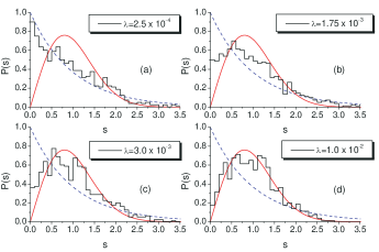
Figure 1: (Color online) Level spacing distributions for: (a) $\lambda=2.5\textrm{ x }10^{-4}$, approximately the location of the local minimum of $\chi^{(1)}(\lambda)$, (b) $\lambda=1.75\textrm{ x }10^{-3}$, approximately the peak of $\chi^{(1)}(\lambda)$, (c) $\lambda=3.0\textrm{ x }10^{-3}$, in the tail of the peak, and (d) $\lambda=1.0\textrm{ x }10^{-2}$, far into the quantum chaotic regime. Here all $800$ well-converged levels are included in the statistics. The Poisson statistics are given by $P(s)=e^{-s}$ (dashed curve) and the Wigner-Dyson statistics are $P(s)=\frac{\pi}{2}se^{-\frac{\pi}{4}s^{2}}$ (solid curve).

In Fig. 2 the eigenenergies are plotted as a function of coupling for two representative intervals of couplings and energies. The changing character of the energy spectrum as a function of the coupling strength is evident. For small couplings, degeneracies are lifted and levels from neighboring sectors begin to cross as the n-mixing regime is entered. As the coupling strength increases further still, the regular n-mixing regime evolves into quantum chaos as level avoidance begins to dominate.

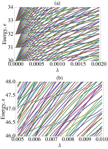
Figure 2: (Color online) Eigenenergies vs. coupling strengths for $K=120$ for (a) couplings $0<\lambda<2\textrm{ x }10^{-3}$ and energies $30<E<34$, such that $0<\eta<2.3$, and (b) couplings $5\textrm{ x }10^{-3}<\lambda<10^{-2}$, such that $10<\eta<23$.

IV.2 The $\chi^{(1)}$ term

Having reviewed the behavior of the level spacings, let us now examine the operator fidelity susceptibility. We start by analyzing $\chi^{(1)}$, first discussing the cut-off approximation:

$$\chi^{(1)}(D_{c})=\frac{2\pi t}{Z(D_{c},\beta)}\sum_{n=1}^{D_{c}}\exp(-\beta E_{n})C_{D_{c}}(n),$$ (17)

where $C_{D_{c}}(n)\equiv\sum_{m=1,m\neq n}^{D_{c}}|\langle n|V|m\rangle|^{2}G_{t}(E_{n}-E_{m})$, $\beta=1/T$, and $Z(D_{c},\beta)\equiv\sum_{n=1}^{D_{c}}\exp(-\beta E_{n}).$ Here $\{|n\rangle\}$ are the $(\frac{K}{2}+1)^{2}$-dimensional or $(\frac{K+1}{2})(\frac{K+1}{2}+1$)-dimensional (for $K$ even, odd respectively) energy eigenvectors of the even parity block of the Hamiltonian $H_{K}$. The number of states included in the sum is called the cut-off dimension, $D_{c}$. Note that if the odd sector were included as well, since the perturbation $V$ preserves parity the sum in (17) would be simply the linear combination of $\chi^{(1)}$ computed over each parity sector. The dependence of all factors on both the coupling $\lambda$ and truncation dimension $K$ has been left implicit. In our calculations we include only the states corresponding to well-converged eigenvalues, namely levels which vary little under additional growth of the truncation dimension $K$. Taking $K=120$, for example, we retain $D_{c}=800$ out of the $3721$ total levels in the even parity sector for the strongest coupling considered, $\lambda=10^{-2}$. Again, though the number of well-converged levels is maximal for smaller couplings, for consistency in our calculations we include the worst-case set of levels for the entire region of interest.

For finite temperature, contributions to the OFS from higher energies are exponentially suppressed due to the coefficient $\rho_{n}=\exp(-\beta E_{n})$ in the outer sum of Eq. (17). This serves to give more weight to the low-energy part of the spectrum for low temperatures, while for high-enough temperatures all levels are included.

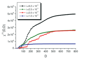
Figure 3: (Color online) Partial sum $\chi^{(1)}(D,D)$ as a function of D, for temperature $T=4.5$ and $\lambda=9.2\textrm{ x }10^{-5},2.5\textrm{ x }10^{-4},2.0\textrm{ x }10^{-3},\textrm{ and }1.0\textrm{ x }10^{-2}$.

In Fig. 3 we show the partial sum $\chi^{(1)}(D_{c})$ as a function of $D_{c}$ for up to $800$ well-converged energy levels, for four different couplings $\lambda$. For example, we can see that a temperature of about $T=4.5$ is sufficient to provide a well-converged result for $\chi^{(1)}$, with the result being better-converged for larger coupling. This is due to an expansion of the energy spectrum towards larger energies as the perturbation strength increases. From now on, we define $\chi^{(1)}$ as the partial sum (17) with $D_{c}=800$.

Let us now look at the parameter dependence of the quantity $\chi^{(1)}(\lambda)$ for finite temperature, plotted in Fig. 4. Recall from Ref. LSWZ that $\chi^{(1)}(\lambda)$ characterizes the variation of the eigenstates, and as shown in Eq. (5) is a function of all level spacings or gaps. The plot is jagged due to the strong contributions of individual level crossings or near misses. However, one may identify two inflection points. For small couplings there is a local minimum of $\chi^{(1)}$, while for progressively larger couplings a global maximum appears. Past the global maximum, $\chi^{(1)}$ decreases as level avoidance begins to appear. From then on, as the couplings grow further $\chi^{(1)}$ continues to decrease.

Our explanation is the following. For vanishing coupling the nearly degenerate subsectors of the spectrum give a large contribution to $\chi^{(1)}$ due to small arguments to $G_{t}(E_{n}-E_{m})$ and significant couplings $|\langle n|V|m\rangle|$ between neighboring levels. However, a slight increase of the coupling lifts those degeneracies, taking the system to the regime where perturbation theory applies since level crossings are rare (see Fig. 2a), and consequently $\chi^{(1)}$ is reduced. Continuing to increase the coupling, the energy levels between subsectors now begin to cross as one enters the so-called n-mixing regime. With sufficiently large coupling the system finally enters the quantum chaotic regime, where couplings between neighboring levels now lead to avoided level crossings, infrequent level crossings, and a consequent decrease in $\chi^{(1)}$. Note that the perturbative regime, for example, persists for a wider range of couplings for low energies than for higher energies, so the system is never entirely in one regime or another. This can be seen by comparing the energies and couplings with the classical chaos parameter $\eta=\lambda\epsilon^{2}$. For the hydrogen atom, higher energies result in a greater susceptibility of the electron to the external magnetic field over the Coulomb potential.

In addition to taking a finite-temperature Gibbs state $\rho=e^{-\beta H}/Z$, another natural choice for the density matrix $\rho$ is to consider the limit $T\to\infty$. In this case our density matrix becomes proportional to a projector $P$ over the subspace spanned by those eigenstates having well-converged eigenvalues. Acting on this well-converged subspace, the state will have the form $\rho_{\infty}=\mathbb{I}/D_{c}$. The result for $\chi_{\infty}^{(1)}$ is plotted as a function of $\lambda$ in Figs. 4 and 5. With this form of the state we see that the contrast between the various regimes is enhanced. Moreover, this state uniformly weights the contributions of many more levels than the low-temperature case, suggesting that variation of $\chi_{\infty}^{(1)}$ may more closely mirror the level spacing statistics. It turns out that increasing the temperature strictly increases the magnitude of $\chi^{(1)}$, so that the “infinite”-temperature case of $\rho=\mathbb{I}/D_{c}$ has the largest value. Moreover, the location of the initial local minimum for small couplings shifts toward smaller values as temperature is increased. This is due to the sampling of higher energy levels, for which smaller couplings are required to traverse the various regimes.

We can thus conclude that, as has already been found for the Dicke model in GZ , the $\chi^{(1)}$ part of the OFS correctly incorporates information about the level spacing statistics for the case of the nonlinearly coupled oscillators. As shown in Fig. 5, modifying the time $t$ does not qualitatively change the plot of $\chi_{\rho}^{(1)}$. Noting the definition of $G_{t}(x)$ following equation (5), where $\lim_{t\to\infty}G_{t}(x)=\delta(x)$, a larger time enhances the contributions to the sum due to level crossings or quasi- level crossings. The growth of $\chi^{(1)}$ for larger times thus reflects its sensitivity to the presence (absence) of level crossings, and hence the transition from regularity to chaos.

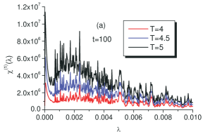
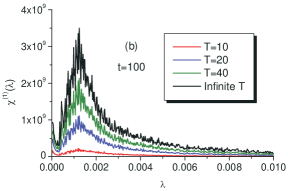
Figure 4: (Color online) The first term of the OFS, $\chi^{(1)}(\lambda)$, with $K=120$, $D_{c}=800$, and $t=100$ for (a) small temperatures and (b) higher temperatures.

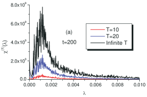
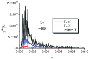
Figure 5: (Color online) The first term of the OFS, $\chi^{(1)}(\lambda)$, with $K=120$, $D_{c}=800$, and various high temperatures at (a) $t=200$ (b) $t=400$.

IV.3 The $\chi^{(2)}$ term

So far we have treated the part of the OFS, $\chi^{(1)}(\lambda)$, which reflects the variation of the eigenstates and depends on the level spacings. The other term, $\chi^{(2)}(\lambda)$, is proportional to the variance of the diagonal elements of the perturbation $V=\partial_{\lambda}H$ with respect to $\rho$ in the energy basis. In Fig. 6 one sees that $\chi^{(2)}$ rapidly decreases with coupling strength. The values of $\chi^{(1)}$ and $\chi^{(2)}$ in both the regular and chaotic regimes differ by about two orders of magnitude, and this is not qualitatively affected by temperature change. This consideration allows us to conclude that for this model the dominant contribution to the overall OFS is given by the fluctuations of the diagonal part of the perturbation $\hat{V}$. However, though the contribution from $\chi^{(1)}$ in this case is relatively small, it possesses a richer functional dependence on the coupling. In particular, while $\chi^{(2)}$ decreases monotonically in the studied parameter interval, $\chi^{(1)}$ reflects the transition through the three described regimes.

In the special case where the diagonal part of the perturbation in the energy basis, $V_{d}$, is zero, this second term will clearly vanish ProsenLoshmidtDynamics . Thus, for an experiment or theoretical treatment in which it is desired that $\chi_{\rho}^{(1)}$ be isolated, choosing a perturbation of this form will eliminate $\chi_{\rho}^{(2)}$.

Our results show that the behavior of the total OFS as a function of the parameter that drives the transition from the regular regime to a chaotic one encodes the already-mentioned resilience of the quantum evolutions to small non-random perturbations even for specific systems. Indeed, for our model the statistical distinguishability between neighboring evolutions decreases with $\lambda$, showing that the resilience of the system to perturbations dramatically increases when it becomes chaotic.

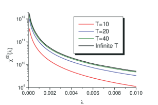
Figure 6: (Color online) The second term of the OFS, $\chi^{(2)}(\lambda)$, taking $K=120$, $D_{c}=800$, and $t=100$

V Conclusion

In this work we have used an operator-geometric quantity, the operator fidelity susceptibility (OFS), to study the transition from regularity to quantum chaos for a pair of coupled two-dimensional harmonic oscillators. This model is equivalent to a hydrogen atom in a uniform external magnetic field, one of the prototypical systems for which both the regimes of classical and quantum chaos have been well-documented theoretically and experimentally. We have seen that, by computing the state-dependent part of the OFS, denoted $\chi^{(1)}(\lambda)$, as a function of the coupling strength $\lambda$ one may distinguish three regimes in parameter space: perturbative, n-mixing, and quantum chaotic. A local minimum for small coupling strength corresponds to the boundary between the perturbative and n-mixing regimes, while the global maximum coincides with the occurrence of level crossings typical of a regular regime. As the level spacing statistics transform from Poisson (maximum likelihood of level crossing) to Wigner-Dyson (vanishing probability of level crossings), $\chi^{(1)}(\lambda)$ correspondingly decreases. We may therefore conclude that $\chi^{(1)}(\lambda)$ both incorporates the information relative to the statistics of the spacings between neighboring energy levels and the information-theoretic notion of distinguishability between quantum evolutions. Our analysis shows that both the distinct elements of the OFS and the OFS as a whole are therefore effective tools for discriminating the different characters, i.e. regular vs. chaotic, of the various regimes of a system’s parameter space.

We would like to remark that while the OFS approach may not be as efficient computationally as other more direct techniques, i.e. the level spacing statistics, the main goal in this work is to see whether the notion of resilience to perturbation, quantified by the OFS, is a useful one in the context of this well-known model. In the future, it would be interesting to experiment with this approach on models where the connection between classical chaos and energy level statistics breaks down, such as in the odd-parity sector of the lithium atom CourtneyKleppner . Indeed, does the ability of $\chi_{\rho}^{(1)}$ to detect the transition from regularity to chaoticity solely depend upon a corresponding change in the level spacing statistics, or can it serve as a measure for chaoticity in systems without this property?

- (1) F. Haake, Quantum Signatures of Chaos (Springer 2001).
- (2) M. L. Mehta, Random Matrices, (Elsevier 2004)
- (3) D.L. Shepelyansky, Physica D 8, 208 (1983); G. Casati, B.V. Chirikov, I. Guarneri, and D.L. Shepelyansky, Phys. Rev. Lett. 56, 2437 (1986).
- (4) A. Peres, Phys. Rev. A 30, 1610 (1984)
- (5) T. Prosen and M. Žnidarič, J. Phys. A 34, L681 (2001); T. Prosen and M. Žnidarič, J. Phys. A: Math. Gen. 35 1455 (2001); T. Gorin, T. Prosen, and T.H. Seligman, New J. Phys. 6 20 (2004); T. Prosen, Phys. Rev. E 65 036208 (2002)
- (6) C. Mejía-Monasterio, G. Benenti, G.G. Carlo, and G. Casati, Phys. Rev. A 71, 062324 (2005)
- (7) G. Benenti, G. Casati, Phys. Rev. E 79, 025201(R) (2009)
- (8) T. Gorin, T. Prosen, T. H. Seligman, and M. Žnidarič, Phys. Rep. 435 33 (2006)
- (9) P. Giorda and P. Zanardi, Phys. Rev. E 81, 017203 (2010)
- (10) X. Wang, Z. Sun, D. Wang, Phys. Rev. E 79, 012105 (2009)
- (11) X-M Lu, Z. Sun, X. Wang, and P. Zanardi, Phys. Rev. A 78, 032309 (2008)
- (12) P. Zanardi and N. Paunkovič, Phys. Rev. E 74, 031123 (2006); P. Zanardi, P. Giorda, and M. Cozzini, Phys. Rev. Lett. 99, 100603 (2007); L. Campos Venuti, P. Zanardi, Phys. Rev. Lett. 99, 095701 (2007).
- (13) H-Q Zhou and J.P. Barjaktarevič, arXiv:cond-mat/0701608; H-Q Zhou, J.P. Barjaktarevič J. Phys. A: Math. Theor. 41, 412001 (2008)
- (14) W-L You, Y-W Li, and S-J Gu, Phys. Rev. E 76, 022101 (2007)
- (15) O. Bohigas, M.J. Giannoni and C. Schmit, Phys. Rev. Lett. 52, 1 (1984)
- (16) P. Plötz, M. Lubasch and S. Wimberger, arXiv:0909.4333;
- (17) D. Delande, “Chaos in atomic and molecular physics”, Chapter 10 of Les Houches Session LII: Chaos and Quantum Physics, (North-Holland 1991)
- (18) D. Delande and J.C. Gay, Phys. Rev. Lett., 57 2006 (1986)
- (19) D. Delande and J.C. Gay, J. Phys. B 17, L335 (1984); D. Delande, J.C. Gay, J. Phys. B: At. Mol. Phys. 19 L173 (1986).
- (20) Note that the notation for labeling here is the reverse of that of Ref. LSWZ , but is consistent with that of Ref. GZ .
- (21) M. Courtney and D. Kleppner, Phys. Rev. A 53 178 (1996)