Improving Large-scale Convection Zone-to-Corona Models

Abstract

We introduce two new methods that are designed to improve the realism and utility of large, active region-scale 3D MHD models of the solar atmosphere. We apply these methods to RADMHD, a code capable of modeling the Sun’s upper convection zone, photosphere, chromosphere, transition region, and corona within a single computational volume. We first present a way to approximate the physics of optically-thick radiative transfer without having to take the computationally expensive step of solving the radiative transfer equation in detail. We then briefly describe a rudimentary assimilative technique that allows a time series of vector magnetograms to be directly incorporated into the MHD system.

1 Introduction

In this paper, we briefly summarize our efforts to improve our models of quiet Sun and active region magnetic fields in computational domains that include the upper convection zone, photosphere, chromosphere, transition region and low corona within a single computational domain. Our goal is similar to that presented in Abbett (2007) — that is, to develop the techniques necessary to efficiently simulate the spatially and temporally disparate convection zone-to-corona interface over spatial scales sufficiently large to accommodate at least one active region.

The advantage of this type of single-domain modeling is clear. For example, evolving a turbulent convection zone and corona simultaneously in a physically self-consistent way allows for the quantitative study of important physical processes such as flux emergence, submergence and cancellation; the transport of magnetic free energy and helicity into the solar atmosphere; the generation of magnetic fields via a convective dynamo; and the physics of coronal heating.

However, this approach is challenging. The computational domain is highly stratified — average thermodynamic quantities change by many orders of magnitude as the domain transitions from a relatively cool, turbulent regime below the visible surface, to a hot, magnetically-dominated and shock-dominated regime high in the model atmosphere. In addition, the low atmosphere is where the radiation field transitions from being optically thick to optically thin. The chromosphere itself presents an additional challenge, since the radiation field is often decoupled from the thermal pool, particularly in some of the strongest, most energetically important transitions.

There are a number of ways to model the energetics of the convection zone-to-corona system, ranging from approximate, parameterized descriptions of the thermodynamics (see e.g., Fan 2009; Hood et al. 2009), to highly realistic treatments of radiative transfer (see e.g., Martínez-Sykora et al. 2009a, b). Since our objective is to model the coupled system over large spatial scales, our goal is to find the most efficient treatment of the energetics possible that still provides a physically meaningful representation of the dynamic connection between the convection zone and corona.

In order to describe the thermodynamics of the corona, a model should include the effects of electron thermal conduction along magnetic field lines and radiative cooling in the optically-thin limit. In addition, some physics-based or empirically-based source of coronal heating must be present if the model corona is to remain hot. In the convective interior well below the visible surface, radiative cooling can be treated in the diffusion limit. The trick is, how best to describe the effects of optically-thick radiative transfer in the region of the model atmosphere that lies between these two extremes.

The most satisfying approach would be to couple the LTE transfer equation (or non-LTE population and transfer equations) to the MHD system to obtain cooling rates and intensities that could be compared directly to observations. Unfortunately, for large active region or global-scale problems, the computational expense of these techniques remains prohibitive.

In Abbett (2007) we tried the opposite approach — ignore the transfer equation altogether, and develop an artificial, fully parameterized means of approximating surface cooling (in this case, we employed a modified form of Newton cooling). This worked relatively well, provided we carefully calibrated the adjustable parameters to match the average sub-surface stratification of previous, more realistic simulations of magneto-convection where the LTE transfer equation was solved in detail (Bercik, 2002).

Of course, the principle drawback of this approach is that it is ultimately ad hoc and unphysical, and requires other, more realistic simulations as a basis for calibration in order to get meaningful results. We therefore have developed an approximation that is based on the macroscopic radiative transfer equation, and have incorporated this new treatment into our 3D MHD model, RADMHD. We describe this new method in Section 2.

While it is important to treat the energetics of the system in a physically meaningful way, it is also important to remember that the utility of a given simulation ultimately depends on the statement of the problem. For an MHD simulation, this boils down to one’s choice of initial states and boundary conditions. It is of great benefit, for example, to pose a simple, well-defined problem, and set up a numerical experiment that can shed light on what is believed to be the relevant physical processes in an otherwise complex system. For example, important progress has been made in understanding the physics of magnetic flux emergence by studying how idealized twisted flux ropes emerge through highly-stratified model atmospheres (see e.g., Cheung et al. 2007; Fan & Gibson 2004).

Yet the observed evolution of the photospheric magnetic field is often far more complex, particularly in and around CME and flare producing active regions. It is very difficult to set up a simple magnetic and energetic configuration that can initialize a simulation that will faithfully mimic the observed evolution of a real active region. It is desirable to do so, however, since we wish to quantitatively understand the physical mechanisms of energy storage and release, and the transport of magnetic energy and helicity between the convective interior and corona.

To make progress, we could take a cue from meteorologists, and investigate a means to incorporate observational data directly into MHD models. This is not at all straightforward for solar models however, since data is obtained entirely through remote sensing, and not in situ.

To address this challenge, we have developed a simple, rudimentary means of assimilating a time series of vector magnetograms into an MHD model of the photosphere-to-corona system. We briefly summarize this technique in Section 3, and apply it to the specific problem of finding a 3D magnetic field that is as force-free as possible given a single measurement of the vector magnetic field at the photosphere.

2 An Approximate Treatment of Optically Thick Cooling

What follows is a brief description of our approximate treatment of optically-thick radiative cooling in the portion of the computational domain that represents the solar photosphere and chromosphere. In practice, this cooling is incorporated into the MHD system as a source term in the equation that evolves the internal energy per unit volume (Equation 4 of Abbett 2007).

We begin by characterizing the net cooling rate for a volume of plasma at some location within the solar atmosphere:

$$R=\!\int\!d\Omega\!\int\!d\nu\left(\eta_{\nu}-\kappa_{\nu}I_{\nu}\right).$$ (1)

Here, $\nu$ represents frequency, and $\Omega$ solid angle. The emissivity, opacity, and specific intensity are frequency dependent, and are denoted $\eta_{\nu}$, $\kappa_{\nu}$ , and $I_{\nu}$ respectively. Rearranging the order of integration, and defining the source function $S_{\nu}$ as the ratio of the emissivity to opacity, we have

Figure 1: Shown is a comparison of the average temperature stratification between the realistic radiative magneto-convection simulations of Bercik (2002) (crosses), and the RADMHD model convection zone using the new treatment of optically-thick transfer (diamonds).

$$R=\!\int\!d\nu\,\kappa_{\nu}\!\int\!d\Omega\left(S_{\nu}-I_{\nu}\right).$$ (2)

Since the source function is independent of direction, we recast the integral as

$$R=4\pi\!\int\!d\nu\,\kappa_{\nu}\left(S_{\nu}-J_{\nu}\right)$$ (3)

with mean intensity

$$J_{\nu}\equiv\frac{1}{4\pi}\int\!d\Omega\,I_{\nu}.$$ (4)

The formal solution for the specific intensity in the plane-parallel approximation is

$$I_{\nu}(\mu)=\int_{0}^{\infty}d\tau^{\prime}\frac{e^{-|\tau_{\nu}-\tau^{\prime}|/|\mu|}}{|\mu|}S_{\nu}(\tau^{\prime}),$$ (5)

where $\mu$ is the usual cosine angle. Then the mean intensity can be expressed as

$$J_{\nu}=\frac{1}{2}\int_{0}^{\infty}d\tau^{\prime}S_{\nu}(\tau^{\prime})\int_{0}^{1}d\,|\mu|\frac{e^{-|\tau_{\nu}-\tau^{\prime}|/|\mu|}}{|\mu|}.$$ (6)

The integral over $\mu$ can now be evaluated and the mean intensity can be cast as

$$J_{\nu}=\frac{1}{2}\int_{0}^{\infty}d\tau^{\prime}S_{\nu}(\tau^{\prime})E_{1}(|\tau_{\nu}-\tau^{\prime}|),$$ (7)

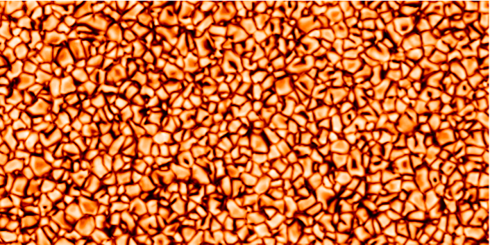
Figure 2: The temperature along a horizontal slice through a RADMHD model photosphere during the relaxation process. This simulation uses the ad hoc Newton cooling described in Abbett (2007) to approximate optically-thick surface cooling. The slice spans $75\times 37.5$ Mm$\,{}^{2}$.

where $E_{1}$ denotes the first exponential integral. So far, this is simply textbook radiative transfer (e.g., Mihalas 1978). No approximations have yet to be made, other than an assumption of a locally plane-parallel atmosphere. Now we’ll make our first approximation. Note that $E_{1}(|\tau_{\nu}-\tau^{\prime}|)$ is singular when $\tau^{\prime}=\tau_{\nu}$, and that the singularity is integrable. Since $E_{1}$ is peaked around $\tau_{\nu}$, contributions from $S_{\nu}(\tau^{\prime})$ will be centered around $S_{\nu}(\tau_{\nu})$. Thus, we approximate the mean intensity by

$$J_{\nu}\approx\frac{1}{2}S_{\nu}(\tau_{\nu})\int_{0}^{\infty}d\tau^{\prime}E_{1}(|\tau_{\nu}-\tau^{\prime}|).$$ (8)

This integral can then be evaluated, giving a simple expression for the mean intensity,

$$J_{\nu}\approx S_{\nu}(\tau_{\nu})\left(1-\frac{E_{2}(\tau_{\nu})}{2}\right),$$ (9)

where $E_{2}$ refers to the second exponential integral. Note that this can be rewritten in the following way:

$$1-\frac{J_{\nu}}{S_{\nu}}\approx\frac{E_{2}(\tau_{\nu})}{2}.$$ (10)

We now return to our expression for the net cooling rate and recast it in a slightly different form,

$$R=4\pi\!\int\!d\nu\,\kappa_{\nu}S_{\nu}\left(1-\frac{J_{\nu}}{S_{\nu}}\right).$$ (11)

Substituting equation 10 into the integrand, we have

$$R\approx 2\pi\!\int\!d\nu\,\kappa_{\nu}S_{\nu}E_{2}(\tau_{\nu}).$$ (12)

If we further assume LTE, the source function is simply the Planck function and we have

$$R\approx 2\pi\!\int\!d\nu\,\kappa_{\nu}B_{\nu}(T)E_{2}(\tau_{\nu}).$$ (13)

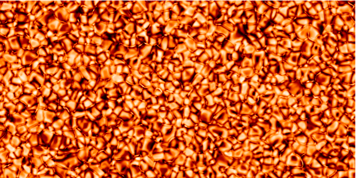
Figure 3: The temperature along a horizontal slice through a RADMHD model photosphere during the relaxation process. In this case, we use our new treatment to approximate the optically-thick surface cooling. We note that the model convection zone has yet to fully relax.

Now for the real swindle! Let’s integrate over frequency, and replace the frequency-dependent opacity by its Planck weighted mean value: That is, replace $\kappa_{\nu}B_{\nu}$ with $\overline{\kappa}(\sigma/\pi)T^{4}$ where $\overline{\kappa}$ represents a Planck-weighted mean opacity, and $\sigma$ the Stefan-Boltzmann constant. Then including the exponential function in the average over frequency, we find that

$$R\approx 2C\,\overline{\kappa}\sigma T^{\,4}E_{2}(\alpha\overline{\tau}).$$ (14)

Here, $C$ represents the normalization constant for the integration. The arbitrary constant $\alpha$ appears in the exponential integral since the mean opacity used in the calculation of the optical depth scale could differ in general from the mean opacity that appears by itself in the integrand.

To determine the normalization constant $C$, we integrate our cooling function from zero to infinity over an isothermal slab to obtain the total radiative flux. The resulting expression must be equal to the known result $F_{tot}=\sigma T^{\,4}$. This allows us to determine the normalization constant $C=\alpha$. To evaluate $\alpha$, we compare the detailed cooling rate depth distribution using this formulation with the cooling rate in the Bercik (2002) LTE model of the solar atmosphere, and conclude the best-fit value is $\alpha=1$ (See Figure 1). Thus, our approximate cooling function takes the form:

$$R\approx 2\,\overline{\kappa}\sigma T^{\,4}E_{2}(\overline{\tau}).$$ (15)

The advantage of this treatment lies in its simplicity. The above approximation for surface cooling, while non-linear, is trivial to calculate for each mesh element. It is certainly more physical than the ad hoc treatment employed in Abbett (2007), since it is based on the radiative transfer equation, and incorporates an optical depth scale into the model. Further, it has no adjustable parameters. The only calibration now required is a choice of optical depth ranges over which to apply the different approximations. Currently, we use the radiative diffusion approximation for optical depths greater than 10, an expression for radiative cooling in the optically-thin limit for optical depths less than 0.1, and the above treatment in the intervening layers.

Figures 2 and 3 provide a qualitative comparison between a model convection zone generated using the ad hoc approach of Abbett (2007) to estimate the effects of optically-thick radiative surface cooling, and one that utilizes the approximation described above. The images represent the gas temperature along a horizontal slice through a RADMHD model photosphere during the relaxation process. Both simulations used the same initial convective state and boundary conditions (periodic in the horizontal directions and closed vertically); the only difference is the treatment of the optically-thick transfer. Distinct differences rapidly develop — the convective cells become more irregularly shaped while the size distribution of cells begins to more closely mimic that of the more realistic simulations of Bercik (2002).

However, there are irregularities in the current data set. For example, there are regions within the intergranular lanes that are hotter than expected. This may be an artifact resulting from our empirically-based coronal heating function (see Abbett 2007 for details) extending unphysically deep into the atmosphere (i.e., its optical depth cutoff is too high), or it may simply be a transient effect that will subside as the simulation progresses. This is a work in progress, and we continue to test and validate the new treatment against our previous quiet Sun simulations, and against more realistic magnetoconvection simulations that treat the LTE transfer equation in detail.

3 Rudimentary Data Assimilation

We now turn our attention to the problem of incorporating a time series of vector magnetic field measurements into our MHD model of the solar atmosphere. The essential problem is that even the most carefully pre-processed sequences of vector magnetograms cannot be expected to exactly satisfy Faraday’s law, and thus are physically inconsistent from the point of view of the numerical model.

This is not particularly surprising, since it is a non-trivial task to properly transform polarization measurements into a vector magnetic field. The datasets naturally suffer from the effects of uncertainty due to noise, seeing, or saturation; the inversion process itself is model dependent; and the well-known 180 degree ambiguity in the transverse field must be resolved in the context of a timeseries of magnetograms rather than in a single magnetogram in isolation.

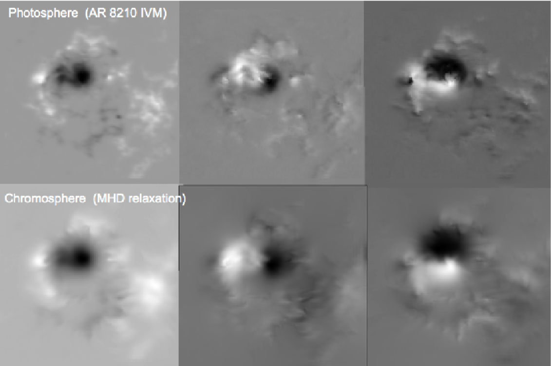
Figure 4: The three components of the magnetic field (from left to right $B_{z}$, $B_{x}$, and $B_{y}$) from the early stages of a 3D RADMHD simulation of NOAA AR 8210. The top row shows a horizontal slice through the model photosphere, and the bottom row shows the magnetic field through a horizontal slice corresponding to the model chromosphere. The top row mirrors the vector magnetic field as measured by the IVM vector magnetograph at Mees Solar Observatory on Haleakala, and the bottom row represents a synthetic chromospheric magnetogram as predicted by the MHD model.

While the data itself presents challenges, it is important to remember that the model suffers from fundamental deficiencies of its own. The single-fluid MHD system may not capture the essential physics of the solar atmosphere, particularly in the low atmosphere where effects such as non-LTE transfer, ion-neutral diffusion, magnetic reconnection, and non-thermal partical acceleration may play fundamental roles in the dynamic evolution of a given region.

Then how shall we proceed? One approach is to take the data at face value and incorporate the measurements directly into an MHD model in the form of time-dependent, characteristic boundary conditions (Wu et al., 2006). Here, one must be mindful to not over-specify the MHD system. This method is restrictive in that only certain components of the electric field or flow inferred from the data can be used to drive the simulation. In addition, one must make assumptions about the thermodynamics of the system in order to drive the model atmosphere in a physical way.

Here, we take another approach. To avoid the mathematical constraints inherent to MHD boundary conditions, we push our lower boundary slightly deeper into the photosphere and instead incorporate the data into the model via additional forces acting on active zones of the calculation where the entire MHD system is being self-consistently evolved.

To do this, we must first obtain an inductive flow field from a given time series of magnetograms that is both consistent with the observed evolution of the vector field and Faraday’s law. This is a non-trivial task, as the problem is inherently under-determined, and the cadence and quality of the magnetograms may vary. There is a growing number of inversion techniques that address this problem (Fisher et al., 2009; Ravindra et al., 2008; Schuck, 2008; Georgoulis & LaBonte, 2006; Welsch et al., 2004; Longcope, 2004; Kusano et al., 2002); each is capable of providing an inductive flowfield consistent with the observations and suitable for incorporation into an MHD model.

Next, we must generate an initial near-equilibrium or steady state atmosphere from the first magnetogram of the timeseries, and choose an appropriate set of exterior boundary conditions. The challenge here is to minimize perpendicular currents within the computational volume, and to provide coronal boundary conditions that minimize forces resulting from magnetic tension. This way, the forces introduced into the model photosphere are the principle drivers of the system.

As a starting point, we generate a non-constant-$\alpha$ force-free extrapolation using a variation of the optimization technique of Wheatland et al. (2000). Given the photospheric magnetogram and a choice of external boundary conditions, this procedure minimizes the functional

$$f=\int dV\;\left(\frac{|({\bf\nabla\times B})\,{\bf\times\,B}|^{2}}{B^{2}}+|{\bf\nabla\cdot B}|^{2}\right),$$ (16)

and generates an initial magnetic configuration.

Unfortunately, the reality is that the photosphere is often far from force-free, making the mathematical problem of generating perfectly force-free equilibia ill-posed. While the optimization technique performs well relative to other methods (see Schrijver et al. 2006), it still cannot be expected to fully converge to an equilibrium state without altering the transverse magnetic field at the photospheric boundary.

We therefore use the optimization method to generate an initial starting point for an MHD relaxation. The above functional need not be vanishingly small in every mesh element, since the MHD code will diffuse away any significant divergence error, and clean up any noisy, unphysical currents near the lower boundary (see Figure 4). In practice, this is done by artificially damping fast-moving waves and allowing the system to slowly evolve to a near-equilibrium state. Of course, the resulting atmosphere is not expected to be force-free near the photosphere. The currents in the system are, however, more physical since they were evolved via the MHD system of conservation equations rather than by attempting to minimize the functional of equation 16.

Our purpose here is not to find a perfectly stable equilibrium solution. In fact, such a state may not exist, given the vector magnetogram and choice of boundary conditions. We are simply striving for an initial atmosphere that is not so vastly out of force balance that motions at the model photosphere are immediately overwhelmed by other less relevant processes. Once this is achieved, we drive the atmosphere in the following way.

First, we define the physical contribution to the force as that described by the MHD momentum conservation equation (see Abbett 2007 for details),

$${\bf F}\equiv-{\bf\nabla\cdot}\left[\rho{\bf uu}\!+\!\left(p+\frac{B^{2}}{8\pi}\right){\bf I}\!-\!\frac{{\bf BB}}{4\pi}\!-\!{\bf\Pi}\right]\!+\!\rho{\bf g}$$ (17)

We then define the forces implied by the data,

$${\bf F}_{data}\equiv\frac{\partial\rho{\bf u}_{\mathrm{inv}}}{\partial t}.$$ (18)

Here, ${\bf u}_{\mathrm{inv}}$ refers to the inductive flow field obtained through one of the many velocity inversion techniques (see Welsch et al. 2007).

Then in a thin volume corresponding to the model’s photosphere, we recast the momentum equation in the following form:

$$\frac{\partial\rho{\bf u}}{\partial t}{\Big{|}}_{phot}=\xi({\bf F}_{data})_{\perp}+\left(1-\xi\right)({\bf F})_{\perp}+({\bf F})_{||}$$ (19)

where the parallel and perpendicular subscripts denote the forces parallel or perpendicular to the direction of the magnetic field. Here, $0<\xi<1$ represents a “confidence matrix” defined at each mesh element within the photospheric volume. It is easy to see that when $\xi=1$, the forces perpendicular to the magnetic field within the model photosphere are determined entirely by the data, and when $\xi=0$, the photospheric layer evolves as the MHD system normally would in the absence of any observational forcing.

Since flows parallel to the field do not affect magnetic evolution, we allow them to evolve in an unconstrained fashion. All other independent variables evolve as prescribed by the MHD system of equations including the magnetic field. Recall, ${\bf u}_{\mathrm{inv}}$ is designed to be consistent with of the observed evolution of one or more components of the photospheric magnetic field (depending on the inversion method used) and, in principle, should drive the photospheric field in a manner consistent with the timeseries of magnetograms.

4 Concluding Remarks

We have developed a rudimentary means of assimilating a time series of vector magnetograms into the interior volume of an MHD model in a manner that is stable, and does not over-specify the problem. We are currently using this assimilative technique to incorporate a timeseries of vector magnetograms into a 120 Mm$\,{}^{3}$ RADMHD model atmosphere that contains a model photosphere, chromosphere, transition region and corona. The IVM data we are using is a four hour timeseries from NOAA AR 8210 — a well-studied flare and CME-producing active region. The simulations are in their preliminary stages, and we hope to report on this work in the near future.

In addition, we have presented a computationally efficient method of approximating optically-thick radiative cooling in our RADMHD quiet Sun models. The treatment improves upon the method of Abbett (2007), while still retaining the efficiency necessary to allow for large, active region-scale, convection zone-to-corona computational domains. Our simulations are progressing, and we are currently evaluating the efficacy and reliability of the new method. We are optimistic that each of these methods will improve the realism and utility of our current suite of numerical models.