Some theoretical results for a class of neural mass equations
Abstract
We study the neural field equations introduced by Chossat and Faugeras in [11] to model the representation and the processing of image edges and textures in the hypercolumns of the cortical area V1. The key entity, the structure tensor, intrinsically lives in a non-Euclidean, in effect hyperbolic, space. Its spatio-temporal behaviour is governed by nonlinear integro-differential equations defined on the Poincaré disc model of the two-dimensional hyperbolic space. Using methods from the theory of functional analysis we show the existence and uniqueness of a solution of these equations. In the case of stationary, i.e. time independent, solutions we perform a stability analysis which yields important results on their behavior. We also present an original study, based on non-Euclidean, hyperbolic, analysis, of a spatially localised bump solution in a limiting case. We illustrate our theoretical results with numerical simulations.
Keywords:
Neural fields; nonlinear integro-differential equations; functional analysis; non-Euclidean analysis; stability analysis; hyperbolic geometry; hypergeometric functions; bumps.
AMS subject classifications: 30F45, 33C05, 34A12, 34D20, 34D23, 34G20, 37M05, 43A85, 44A35, 45G10, 51M10, 92B20, 92C20.
1 Introduction
Chossat and Faugeras in [11] have introduced a new and elegant approach to model the processing of image edges and textures in the hypercolumns of area V1 that is based on a nonlinear representation of the image first order derivatives called the structure tensor. They assumed that this structure tensor was represented by neuronal populations in the hypercolumns of V1 that can be described by equation similar to those proposed by Wilson and Cowan [26].
Our investigations are motivated by the work of Bressloff, Cowan, Golubitsky, Thomas and Wiener [8, 9] on the spontaneous occurence of hallucinatory patterns under the influence of psychotropic drugs and the further studies of Bressloff and Cowan [7, 6, 5]. We hardly think that the natural spatial extension of our model would lead to an exciting anlysis of hyperbolic hallucinatory patterns. But, this requires first to better understand the a-spatial model and this is the subject of this present work. The a-spatial model can also be linked to the work by Ben-Yishai [3] and Hansel, Sompolinsky [16] on the ring model of orientation.
The aim of this paper is to present a general and rigorous mathematical framework for the modeling of neuronal populations in one hypercolumn of V1 by the structure tensor which is based on miscellaneous tools of functional analysis. We illustrate our results with numerical experiments. In section 2 we briefly introduce the equations, in section 3 we analyse the problem of the existence and uniqueness of their solutions. In section 4 we deal with stationary solutions. In section 5, we present an analysis of what we called a hyperbolic radially symmetric stationary-pulse in a limiting case. In the penultimate, we present some numerical simulations of the solutions. We conclude in section 7.
2 The model
We recall that the structure tensor is a way of representing the edges and textures of a 2D image [4, 21]. Moreover, a structure tensor can be seen as a symmetric positive matrix.
We assume that a hypercolumn of V1 can represent the structure tensor in the receptive field of its neurons as the average membrane potential values of some of its membrane pouplations. Let be a structure tensor. The average potential of the column has its time evolution that is governed by the following neural mass equation adapted from [11] where we allow the connectivity function to depend upon the time variable and we integrate over the set of symmetric definite-positive matrices:
| (1) |
The nonlinearity is a sigmoidal function which may be expressed as:
where describes the stiffness of the sigmoid. is an external input.
The set SPD(2) is the set of symmetric positive-definite matrices. It can be seen as a foliated manifold by way of the set of special symmetric positive definite matrices . Indeed, we have: . Furthermore, , where is the Poincare Disk, see e.g. [11]. As a consequence we use the following foliation of SPD(2): , which allows us to write for all , with . , and are related by the relation and the fact that is the representation in of with .
It is well-known [20] that (and hence SSPD(2)) is a two-dimensional Riemannian space of constant sectional curvature equal to -1 for the distance noted defined by
It follows, e.g. [24, 11], that SDP(2) is a three-dimensional Riemannian space of constant sectional curvature equal to -1 for the distance noted defined by
As shown in proposition (A.0.1) of appendix A it is possible to express the volume element in coordinates with :
We rewrite (1) in coordinates:
We get rid of the constant by redefining as .
| (2) |
The aim of the following sections is to establish that (2) is well-defined and to give necessary and sufficient conditions on the different parameters in order to prove some results on the existence and uniqueness of a solution of (2).
3 The existence and uniqueness of a solution
The aim of this section is to give theoretical and general results of existence and uniqueness of a solution of (1). In the first subsection 3.1 we study the simpler case of homogeneous solutions of (1), i.e. of solutions that are constant with respect to the tensor variable . We then we study in 3.2 the useful case of the semi-homogeneous solutions of (1), i.e. of solutions that depend on the tensor variable but only through its coordinate in , and we end up in 3.3 with the general case.
3.1 Homogeneous solutions
A homogeneous solution to (1) is a solution that does not depend upon the tensor variable for a given homogenous input and a constant initial condition . In coordinates, a homogeneous solution of (2) is defined by:
where:
| (3) |
Hence necessary conditions for the existence of a homogeneous solution are that:
-
•
the double integral (3) is convergent,
-
•
does not depend upon the variable . In that case, we note instead of .
In the special case where is a function of only the distance between and :
the second condition is satisfied. We postpone the verification of this fact until the following section. To summarize, the homogeneous solutions satisfy the differential equation:
| (4) |
3.1.1 A first existence and uniqueness result
Equation (2) defines a Cauchy problem and we have the following theorem.
Theorem 3.1.1.
If the external current and the connectivity function are continuous on some closed interval containing , then for all in , there exists a unique solution of (4) defined on a subinterval of containing such that .
Proof.
It is a direct application of Cauchy’ theorem on differential equations. We consider the mapping defined by:
It is clear that is continuous from to . We have for all and :
where .
Since, is continuous on the compact interval , it is bounded there by and:
∎
We can extend this result to the whole time real line if and are continuous on .
Proposition 3.1.1.
If and are continuous on , then for all in , there exists a unique solution of (4) defined on such that .
Proof.
We have already shown the following inequality:
Then is locally Lipschitz with respect to its second argument. Let be a maximal solution on and we denote by the upper bound of . We suppose that . Then we have for all :
where .
But theorem B.0.2 ensures that it is impossible, then . The same proof with the lower bound of gives the conclusion.
∎
3.1.2 Simplification of (3) in a special case
Invariance
In the previous section, we have stated that in the special case where was a function of the distance between two points in , then did not depend upon the variables . We now prove this assumption.
Lemma 3.1.1.
When is only a function of , then does not depend upon the variable .
Proof.
We work in coordinates and we begin by rewritting the double integral (3) for all :
The change of variable yields:
And it establishes that does not depend upon the variable . To finish the proof, we show that the following integral does not depend upon the variable :
| (5) |
where is a real-valued function such that is well defined.
We express in horocyclic coordinates: (see appendix D) and (5) becomes:
With the change of variable , this becomes:
The relation (proved e.g. in [17]) yields:
with and , which shows that does not depend upon the variable , as announced. ∎
Mexican hat connectivity
In this paragraph, we push further the computation of in the special case where does not depend upon the time variable and takes the special form suggested by Amari in [1], commonly referred to as the “Mexican hat” connectivity. It features center excitation and surround inhibition which is an effective model for a mixed population of interacting inhibitory and excitatory neurons with typical cortical connections. It is also only a function of .
In detail, we have:
where:
with and .
In this case we can obtain a very simple closed-form formula for as shown in the following lemma.
Lemma 3.1.2.
When is a mexican hat function of and independent of , then:
| (6) |
where erf is the error function defined as:
Proof.
The proof is given in appendix C. ∎
3.2 Semi-homogeneous solutions
A semi-homogeneous solution of (2) is defined as a solution which does not depend upon the variable . In other words, the populations of neurons are not sensitive to the determinant of the structure tensor. The neural mass equation is then equivalent to the neural mass equation for tensors of unit determinant. We point out that semi-homogeneous solutions were previously introduced by Chossat and Faugeras in [11]. They also performed a bifurcation analysis of what they called H-planforms. In this section, we define the framework in which their equations make sense.
| (7) |
where
We have implicitly made the assumption, that does not depend on the coordinate . Some conditions under which this assumption is satisfied are described below.
We now deal with the problem of the existence and uniqueness of a solution to (7) for a given initial condition. We first introduce the framework in which this equation makes sense.
3.2.1 The well-posedness of equation (7)
Let be an open interval of . We assume that:
-
•
(C1): , ,
-
•
(C2): where is defined as for all
, -
•
(C3): where .
Note that conditions (C1)-(C2) and lemma 3.1.1 imply that for all , . And then, for all , the mapping is integrable on . We deduce that for all :
The last inequality is a consequence of lemma 3.1.1 which shows that is not a function of .
Finally for all and , the righthand side of equation (7) is well-defined.
We introduce the following mapping, defined on , where is a yet to be defined functional space:
| (8) |
Our aim is to find a functional space where (8) is well-defined and the function maps to for all s.
A natural choice would be to choose as a -integrable function of the space variable with . Unfortunately, the homogeneous solutions (constant with respect to ) do not belong to that space. Moreover, a valid model of neural networks should only produce bounded membrane potentials. That is why we focus our choice on functional spaces of bounded, or essentially bounded, functions.
The well-posedness of equation (7) in the case
Our first choice is . The Fischer-Riesz’s theorem ensures that is a Banach space for the norm: . We have the following proposition.
Proposition 3.2.1.
If satisfies conditions (C1)-(C3) then is well defined and is from to .
Proof.
The well-posedness of equation (7) in the case
We now choose the space of the bounded continuous functions on . As shown in, e.g. [18], this is a Banach space with respect to the uniform norm: . The previous proposition 3.3.1 still holds:
Proposition 3.2.2.
If satisfies conditions (C1)-(C3) then is well defined and is from to .
Proof.
For all and :
so is bounded. It remains to show that for all the mapping is continuous on . We fix and write in horocyclic coordinates with and define on as:
A method similar to the one used in section 3.1.2 leads to:
We now use a theorem on integrals depending on a parameter. It is easy to verify that
-
1.
for all the function is measurable on ,
-
2.
for almost every the function is continuous on ,
-
3.
for all ,
and is integrable on .
It follows that the function is continuous on and is continuous on .
Finally, belongs to .
∎
3.2.2 The existence and uniqueness of a solution of (7)
From now on, is a functional Banach space for the norm . We suppose that all the hypotheses are verified so that is well-defined from to with an open interval containing . In the previous section we have already presented two different examples for : and .
We rewrite (7) as a Cauchy problem defined on :
| (9) |
Theorem 3.2.1.
If the external current belongs to with an open interval containing and satisfies conditions (C1)-(C3), then for all , there exists a unique solution of (9) defined on a subinterval of containing .
Proof.
We prove that is continuous on . We have
and therefore
Because of condition (C2) we can choose small enough so that
is arbitrarily small. This proves the continuity of . Moreover it follows from the previous inequality that:
with . This ensures the Lipschitz continuity of with respect to its second argument, uniformly with respect to the first. The Cauchy-Lipschitz theorem on a Banach space yields the conclusion. ∎
This solution, defined on the subinterval of can in fact be extended to the whole real line, and we have the following proposition.
Proposition 3.2.3.
If the external current belongs to and satisfies conditions (C1)-(C3) with , then for all , there exists a unique solution of (9) defined on .
3.2.3 The boundedness of a solution of (7)
We assume that is a Banach space chosen so that the mapping is well defined from to . Then the following propostion holds.
Proposition 3.2.4.
If the external current belongs to and is bounded in time, i.e. , and satisfies conditions (C1)-(C3) with , then the solution of (9) is bounded for each initial condition .
Proof.
For all we integrate (7) over :
The following upperbound holds
| (10) |
and hence
which shows that the solution is bounded for each initial condition .
∎
The upperbound (10) yields a simple attracting set for the dynamics of (7) as shown in the following proposition.
Proposition 3.2.5.
Let . The open ball of of center and radius is stable under the dynamics of equation (7). Moreover it is an attracting set for this dynamics and if and then:
3.3 General solution
We now deal with the general solutions of equation (1). We first give some hypotheses that the connectivity function must satisfy. We present them in two ways, first on the set of structure tensors considered as the set SPD(2) and, second on the set of tensors seen as . Let be a subinterval of . We assume that:
-
•
(H1): , ,
-
•
(H2): where is defined as for all where is the identity matrix of ,
-
•
(H3): , where .
We now express these hypotheses for the representation in of structure tensors:
-
•
(H1bis): , ,
-
•
(H2bis): where is defined as for all ,
-
•
(H3bis): , where
.
3.3.1 Functional space setting
We need to settle on the choice of a Banach functional space for the membrane potential as in section 3.2.
Our study of the semi-homogeneous case suggests the following choice: . As is an open set of , is a Banach space for the norm: .
We introduce the following mapping such that:
| (12) |
Proposition 3.3.1.
If with and satisfies hypotheses (H1bis)-(H3bis) then is well-defined and is from to .
Proof.
, we have:
∎
3.3.2 The existence and uniqueness of a solution of (2)
We rewrite (2) as a Cauchy problem:
| (13) |
Theorem 3.3.1.
If the external current belongs to with an open interval containing and satisfies hypotheses (H1bis)-(H3bis), then fo all , there exists a unique solution of (13) defined on a subinterval of containing such that for all .
Proof.
The proof is a direct adaptation of the proof of theorem 3.2.1. ∎
Proposition 3.3.2.
If the external current belongs to and satisfies hypotheses (H1bis)-(H3bis) with , then for all , there exists a unique solution of (13) defined on such that for all .
Proof.
The proof is readily adapted from that of proposition 3.2.3. ∎
3.3.3 The intrinsic boundedness of a solution of (2)
In the same way as in the homogeneous case, we show a result on the boundedness of a solution of (2). The proofs of the following properties are exactely the same as those in section 3.2.3.
Proposition 3.3.3.
If the external current belongs to and is bounded in time and satisfies hypotheses (H1bis)-(H3bis) with , then the solution of (13) is bounded for each initial condition .
If we set:
where . The following corollary is a consequence of the previous proposition.
Corollary 3.3.1.
If and then:
4 Stationary solutions
We look at the equilibrium states, noted of (2), when the external input and the connectivity do not depend upon the time. We assume that satisfies hypotheses (H1bis)-(H2bis). We redefine for convenience the sigmoidal function to be:
so that a stationary solution (independent of time) satisfies:
| (14) |
We define the nonlinear operator from to , noted , by:
| (15) |
Finally, (14) is equivalent to:
4.1 Study of the nonlinear operator
We recall that we have set for the Banach space and proposition 3.3.1 shows that . We have the further properties:
Proposition 4.1.1.
satisfies the following properties:
-
•
for all ,
-
•
is continuous on ,
Proof.
The first property was shown to be true in the proof of theorem 3.2.1. The second property follows from the following inequality:
∎
We denote by and the two operators from to defined as follows for all and all :
| (16) |
and
where is the Heaviside function.
It is straightforward to show that both operators are well-defined on and map to . Moreover the following proposition holds.
Proposition 4.1.2.
We have
Proof.
It is a direct application of the dominated convergence theorem using the fact that:
∎
4.2 The convolution form of the operator in the semi-homogeneous case
It is convenient to consider the functional space to discuss semi-homogeneous solutions. A semi-homogeneous persistent state of (2) is deduced from (14) and satisfies:
| (17) |
where the nonlinear operator from to is defined for all and by:
We define the associated operators, :
We rewrite the operator in a convenient form by using the convolution in the hyperbolic disk. First, we define the convolution in a such space. Let denote the Haar measure on the group (see [17]), normalized by:
for all functions of . Given two functions in we define the convolution by:
We recall the notation .
Proposition 4.2.1.
For all and we have:
| (18) |
Proof.
We only prove the result for . Let , then:
and for all , so that:
∎
Let be a point on the circle . For , we define the “inner product” to be the algebraic distance to the origin of the (unique) horocycle based at through (see [11]). Note that does not depend on the position of on the horocycle. The Fourier transform in is defined as (see [17]):
for a function such that this integral is well-defined.
Lemma 4.2.1.
The Fourier transform in , of does not depend upon the variable .
Proof.
For all and ,
We recall that for all is the rotation of angle and we have , and , then:
∎
We now introduce two functions that enjoy some nice properties with respect to the Hyperbolic Fourier transform and are eigenfunctions of the linear operator .
Proposition 4.2.2.
Let and then:
-
•
-
•
Proof.
We begin with and use the horocyclic coordinates. We use the same changes of variables as in lemma 3.1.1:
By rotation, we obtain the property for all .
For the second property [17, Lemma 4.7] shows that:
∎
A consequence of this proposition is the following lemma.
Lemma 4.2.2.
The linear operator is not compact and for all , the nonlinear operator is not compact.
Proof.
The previous proposition 4.2.2 shows that has a continuous spectrum which iimplies that is not a compact operator.
Let be in , for all we differentiate and compute its Frechet derivative:
If we assume further that does not depend upon the space variable , we obtain:
If was a compact operator then its Frechet derivative would also be a compact operator, but it is impossible. As a consequence, is not a compact operator. ∎
4.3 The convolution form of the operator in the general case
We adapt the ideas presented in the previous section in order to deal with the general case. We recall that if is the group of positive real numbers with multiplication as operation, then the Haar measure is given by . For two functions in we define the convolution by:
We recall that we have set by definition: .
Proposition 4.3.1.
For all and we have:
| (19) |
Proof.
Let be in . We follow the same ideas as in proposition 4.2.1 and prove only the first result. We have
∎
We next assume further that the function is separable in , and more precisely that where and for all . The following proposition is an echo to proposition 4.2.2.
Proposition 4.3.2.
Let , and then:
-
•
-
•
where is the usual Fourier transform of .
Proof.
A straightforward consequence of this proposition is an extension of lemma 4.2.2 to the general case:
Lemma 4.3.1.
The linear operator is not compact and for all , the nonlinear operator is not compact.
4.4 The set of the solutions of (14)
Let the set of the solutions of (14) for a given slope parameter :
We have the following proposition.
Proposition 4.4.1.
If the input current is equal to a constant , i.e. does not depend upon the variables then for all , . In the general case , if the condition is satisfied, then .
Proof.
Due to the properties of the sigmoid function, there always exists a constant solution in the case where is constant. In the general case where , the statement is a direct application of the Banach fixed point theorem, as in [13]. ∎
Remark 4.4.1.
It should be clear that if the input current does not depend upon the variables and if the condition is satisfied, then there exists a unique stationary solution which, in effect, does not depend upon the variables .
If on the other hand the input current does depend upon these variables, is invariant under the action of a subgroup of , the group of the isometries of (see (D)), and the condition is satisfied, then the unique stationary solution will also be invariant under the action of the same subgroup.
When the condition is satisfied we call primary stationary solution the unique solution in .
4.5 Stability of the primary stationary solution
In this subsection we show that the condition guarantees the stability of the primary stationary solution to (2).
Theorem 4.5.1.
We suppose that and that the condition is satisfied, then the associated primary stationary solution of (2) is asymtotically stable.
Proof.
Let be the primary stationary solution of (2), as is satisfied. Let also be the unique solution of the same equation with some initial condition , see theorem 3.2.1. We introduce a new function which satisfies:
where and the vector is given by with . We note that, because of the definition of and the mean value theorem . This implies that for all .
If we set: , then we have:
and is continuous for all . The Gronwall inequality implies that:
and the conclusion follows.
∎
5 Spatially localised bumps in the high gain limit
In many models of working memory, transient stimuli are encoded by feature-selective persistent neural activity. Such stimuli are imagined to induce the formation of a spatially localised bump of persistent activity which coexists with a stable uniform state. As an example, Camperi and Wang [10] have proposed and studied a network model of visuo-spatial working memory in prefontal cortex adapted from the ring model of orientation of Ben-Yishai and colleagues [3]. It is therefore natural to study the emergence of spatially localised bumps for the structure tensor model in a hypercolumn of V1. We only deal with the reduced case of equation (7) and keep the general case for future work.
In order to construct exact bump solutions, we consider the high gain limit of the sigmoid function. As above we denote by the Heaviside function defined by for and otherwise. Equation (7) is rewritten as:
| (20) |
We make the assumption that the system is spatially homogeneous that is, the external input does not depend upon the variables and the connectivity function depends only on the hyperbolic distance between two points of : . We also introduce a threshold to shift the zero of the Heaviside function.
5.1 Stationary pulses
Our aim is to construct a hyperbolic radially symmetric stationary pulse. Let us first consider a general stationary pulse:
We assume that the set is compact. We note the integral . The relation holds for all .
In order to calculate , we use the Fourier transform. First we rewrite as a convolution product:
where .
In [17], Helgason proves an inversion formula for the hyperbolic Fourier transform and we apply this result to .
| (21) |
Then,
It appears that the study of consists in calculating the convolution product .
Let for we have:
for all , so that:
5.1.1 Study of when
We now consider the special case where is a hyperbolic disk centered at the origin of hyperbolic radius , noted .
First step
We start by giving an explicit formula for a useful integral.
Lemma 5.1.1.
For all the following formula holds:
where is the hyperbolic ball and:
where and is the hypergeometric function of first kind.
Proof.
We write in hyperbolic polar coordinates, (see appendix D). We have:
Because of the above definition of , this reduces to
In [17] Helgason proved that:
with . We then use the formula obtained by Erdelyi in [12]:
Using some simple hyperbolic trigonometry formulae we obtain:
from which we deduce
Finally we use the equality shown in [12]:
In our case we have: and , so , . We obtain
Since Hypergeometric functions are symmetric with respect to the first two variables:
we write
which yields the announced formula
∎
Second step
In this paragraph, we show that the mapping is a radial function, i.e. it depends only upon the variable . We then show that .
Proposition 5.1.1.
If and is written with in hyperbolic polar coordinates the integral depends only upon the variable .
Proof.
If , then and . Similarly . We can write
which, as announced, is only a function of . ∎
We now give an explicit formula for the integral . We first recall a formula from [17].
Lemma 5.1.2.
For all the following equation holds:
Proof.
See [17]. ∎
It follows immediately that for all and we have:
We integrate this formula over the hyperbolic ball which gives:
and we exchange the order of integration:
We note that the integral does not depend upon the variable . Indeed:
and indeed the integral does not depend upon the variable :
Finally, we can write:
because (as solutions of the same equation).
This completes the proof that:
| (22) |
The main result
At this point we have proved the following proposition.
Proposition 5.1.2.
If and , is given by the following formula:
| (23) |
where
| (24) |
We are now in a position to obtain an analytic form for . It is given in the following theorem.
Theorem 5.1.1.
For all :
| (25) |
Discussion
Let us point out that our result can be linked to the work of Folias and Bressloff in [15]. They constructed a two-dimensional pulse for a general, radially symmetric synaptic weight function. They obtain a similar formal representation of the integral of the connectivity function over the disk centered at the origin and of radius . Using their notations,
where is the Bessel function of the first kind and is the real Fourier transform of . In our case, instead of the Bessel function, we find which is linked to the hypergeometric function of the first kind, as explained in lemma 5.1.1.
We next adapt the results proved by Folias and Bressloff in [15] to the hyperbolic case.
5.1.2 A hyperbolic radially symmetric stationary-pulse
We note a hyperbolic radially symmetric stationary-pulse solution of (20) where depends only upon the variable and is such that:
and
Substituting into (20) yields:
| (26) |
where is defined in equation (25) and is a Gaussian input.
The condition for the existence of a stationary pulse is given by:
| (27) |
where
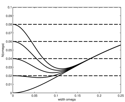
The function is plotted in figure 1 for a range of the input amplitude . The horizontal dashed lines indicate different values of , the points of intersection determine the existence of stationary pulse solutions.
We now show that for a general monotonically decreasing weight function , the function is necessarily a monotonically decreasing function of . This will ensure that the hyperbolic radially symmetric stationary-pulse solution (26) is also a monotonically decreasing function of in the case of a Gaussian input. Differentiating with respect to yields:
We have to compute
It is result of elementary hyperbolic trigonometry that
we let , and define
It follows that
and
We conclude that if then for all and
which implies for , since .
To see that it is also negative for , we differentiate equation (25) with respect to :
The following formula holds for the hypergeometric function (see Erdelyi in [12]):
It implies
Substituting in the previous equation giving we find:
implying that:
Consequently, for . Hence is monotonically decreasing in for any monotonically decreasing synaptic weight function .
5.1.3 Linear stability analysis
We now analyse the evolution of small time-dependent perturbations of the hyperbolic stationary-pulse solution through linear stability analysis.
Spectral analysis of the linearized operator
Equation (20) is linearized about the stationary solution by introducing the time-depndent perturbation:
This leads to the linear equation:
We separate variables by setting to obtain the equation:
Introducing the hyperbolic polar coordinates and using the result:
we obtain:
With a slight abuse of notation we are led to study the solutions of the integral equation:
| (28) |
where:
Essential spectrum
If the function satisfies the condition
then equation (28) reduces to:
yielding the eigenvalue:
This part of the essential spectrum is negative and does not cause instability.
Discrete spectrum
If we are not in the previous case we have to study the solutions of the integral equation (28).
This equation shows that is completely determined by its values on the circle of equation . Hence, we need only to consider , yielding the integral equation:
The solutions of this equation are exponential functions , where satisfies:
By the requirement that is -periodic in , it follows that , where . Thus the integral operator with kernel has a discrete spectrum given by:
is real since:
Hence,
Since is a positive function of , it follows that:
Stability of the hyperbolic stationary pulse requires that for all , . This can be rewritten as:
Using the fact that for all , we obtain the reduced stability condition:
where
From (26) we have:
where
We have previously established that and is negative by definition. Hence, letting , we have
By substitution we obtain another form of the reduced stability condition:
| (29) |
We also have:
and
showing that the stability condition (29) is satisfied when and is not satisfied when .
6 Numerical results
The aim of this section is to numerically solve (7) for different values of the parameters. This implies developing a numerical scheme that approaches the solution of our equation, and proving that this scheme effectively converges to the solution.
Since equation (7) is defined on , computing the solutions on the whole hyperbolic disk has same the complexity as computing the solutions of usual Euclidean neural field equations defined on . As most authors in the Euclidean case [15, 22, 23, 25], we reduce the domain of integration to a compact region of the hyperbolic disk. Practically, we work on the Euclidean ball of radius and center . Note that a Euclidean ball centered at the origin is also a centered hyperbolic ball, their radii being different.
We have divided this section in four parts. The first part is dedicated to the study of the discretization scheme of equation (7). In the following three parts, we study the solutions of different connectivity functions: exponential function 6.2, Gabor function 6.3 and a difference of Gaussians function LABEL:subsection:gaussian.
6.1 Numerical schemes
Let us consider the modified equation of (7):
| (30) |
We assume that the connectivity function satisfies the conditions (C1)-(C2). Moreover we express in (Euclidean) polar coordinates such that , and . The integral in equation (30) is then:
We define to be the rectangle .
6.1.1 Discretization scheme
We discretize in order to turn (30) into a finite number of equations. For this purpose we introduce , and , ,
and obtain the equations:
which define the discretization of (30):
| (31) |
where 111 is the space of the matrices of size with real coefficients., . Similar definitions apply to and . Moreover:
It remains to discretize the integral term. For this as in [14], we use the rectangular rule for the quadrature so that for all we have:
We end up with the following numerical scheme, where (resp. ) is an approximation of (resp. ), :
with .
6.1.2 Discussion
We discuss the error induced by the rectangular rule for the quadrature. Let be a function which is on a rectangular domain . If we denote by this error, then where and are the number of subintervals used and where, as usual, is a multi-index. As a consequence, if we want to control the error, we have to impose that the solution is, at least, in space.
Four our numerical experiments we use the specific function of Matlab which is based on an explicit Runge-Kutta (4,5) formula (see [2] for more details on Rung-Kutta methods).
We can also establish a proof of the convergence of the numerical scheme which is exactly the same as in [14] excepted that we use the theorem of continuous dependence of the solution for ordinary differential equations.
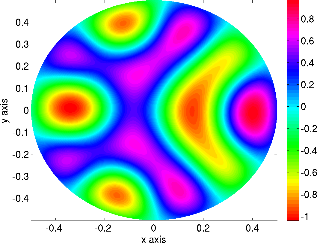
6.2 Purely excitatory exponential connectivity function
In this subsection, we give some numerical solutions of (7) in the case where the connectivity function is an exponential function, , with a positive parameter. Only excitation is present in this case. In all the experiments we set and with .
Constant input
We fix the external input to be of the form:
In all experiments we set and , this means that the input has a sharp profile centered at .
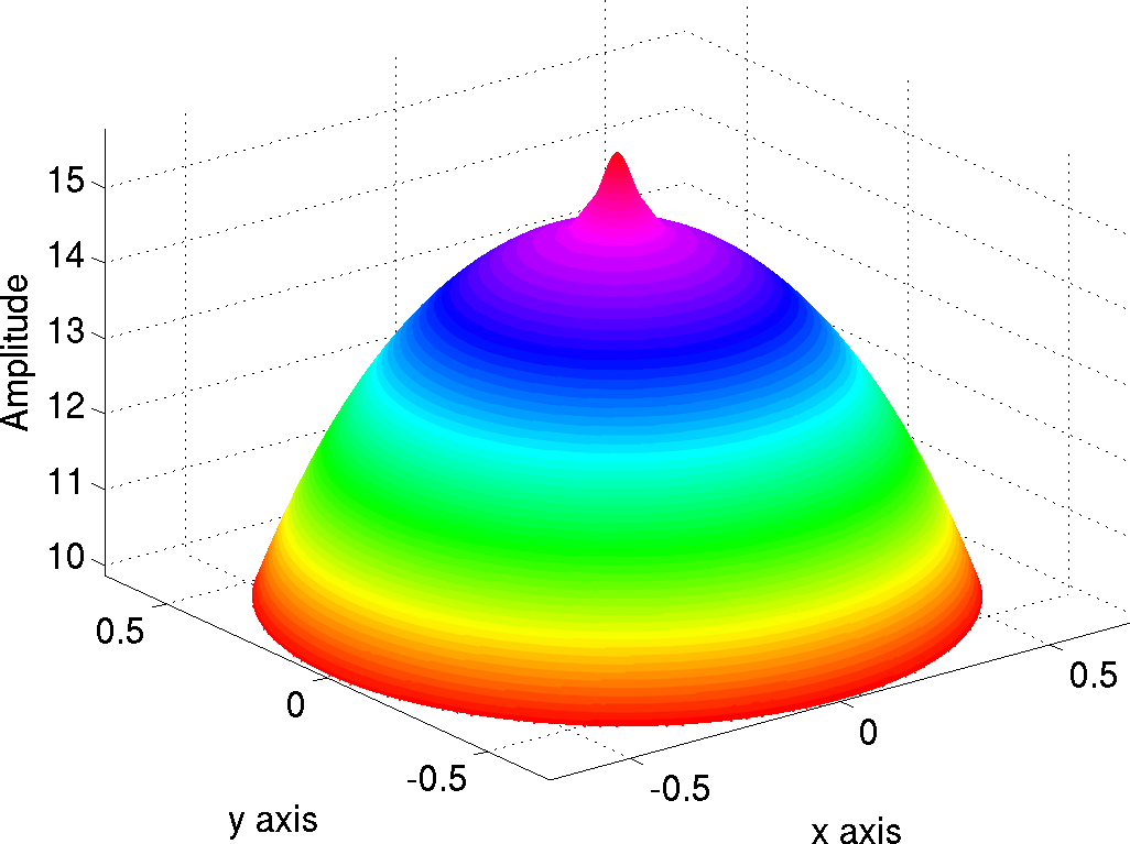
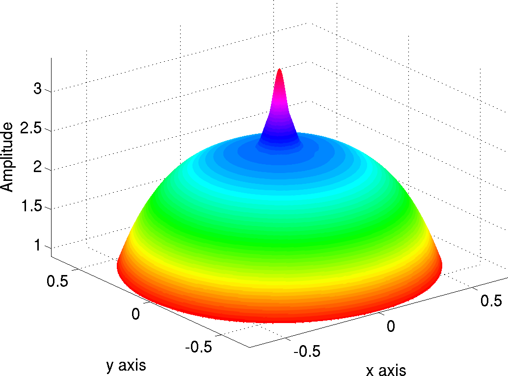
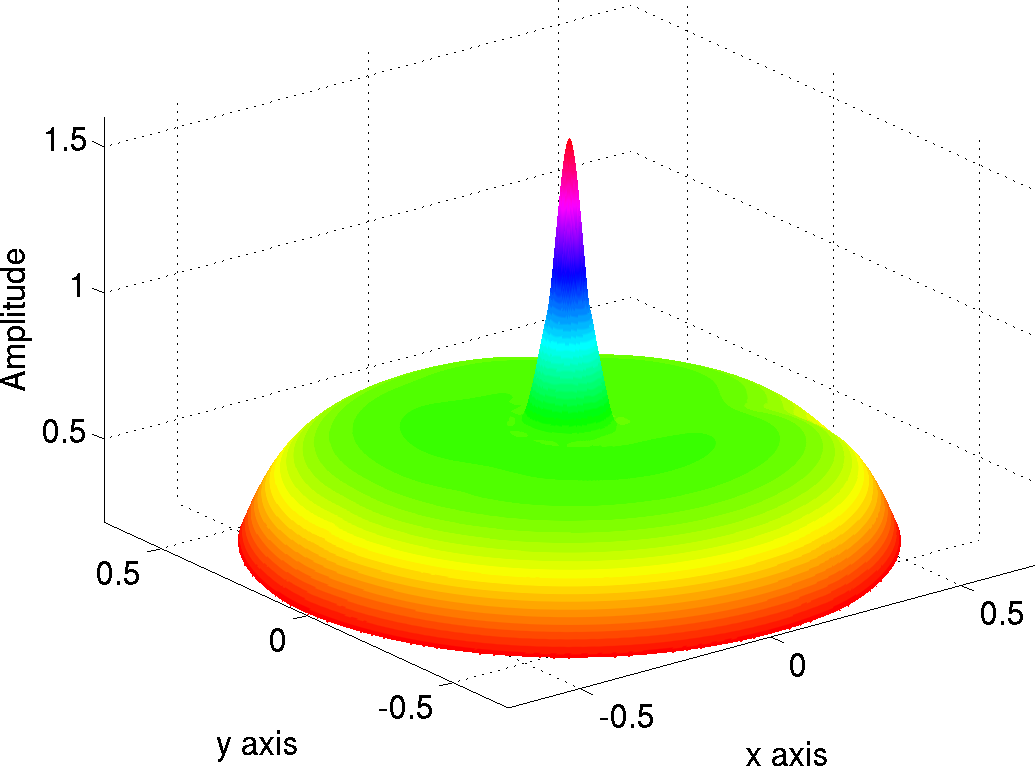
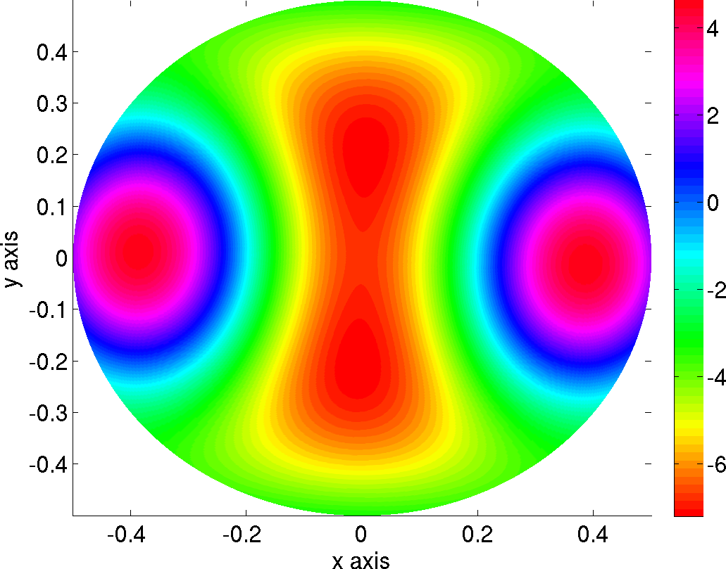
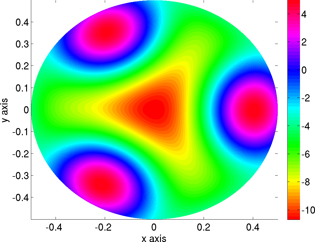
We show in figure 2 plots of the solution at time for three different values of the width of the exponential function. When , the whole network is hightly excited, see figure 2(a). When changes from to the amplitude of the solution decreases, and the area of high excitation becomes concentrated around the external input.
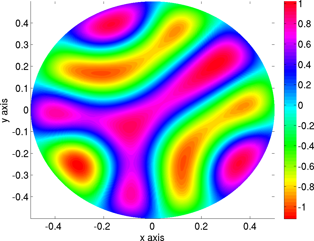
Variable input
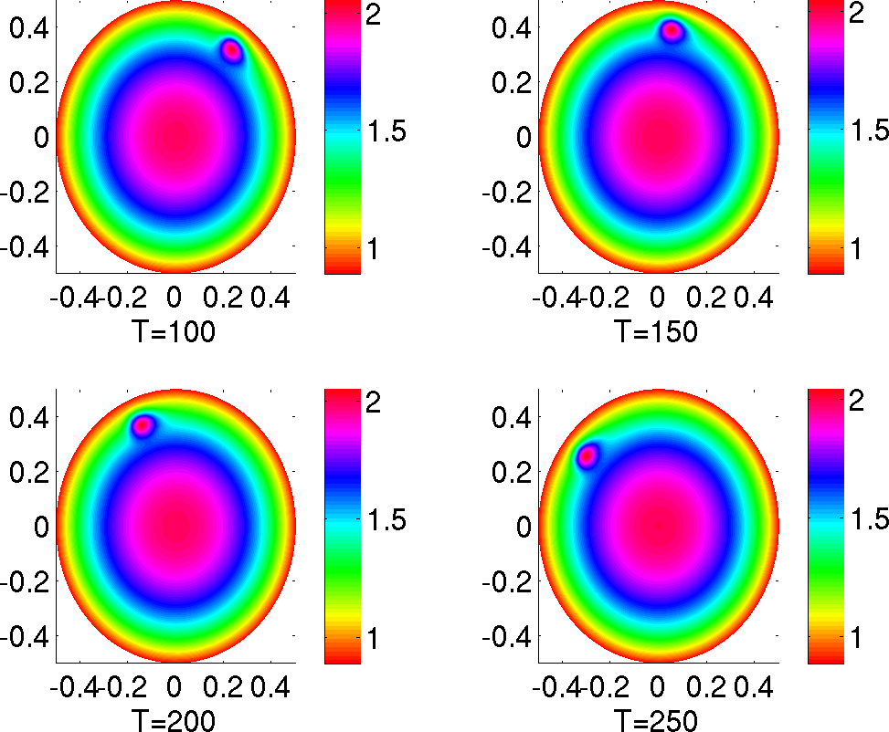
In this paragraph, we allow the external current to depend upon the time variable. We have:
where . This is a bump rotating with angular velocity around the circle of radius centered at the origin. In our numerical experiments we set , , and . We plot in figure 3 the solution at different times .
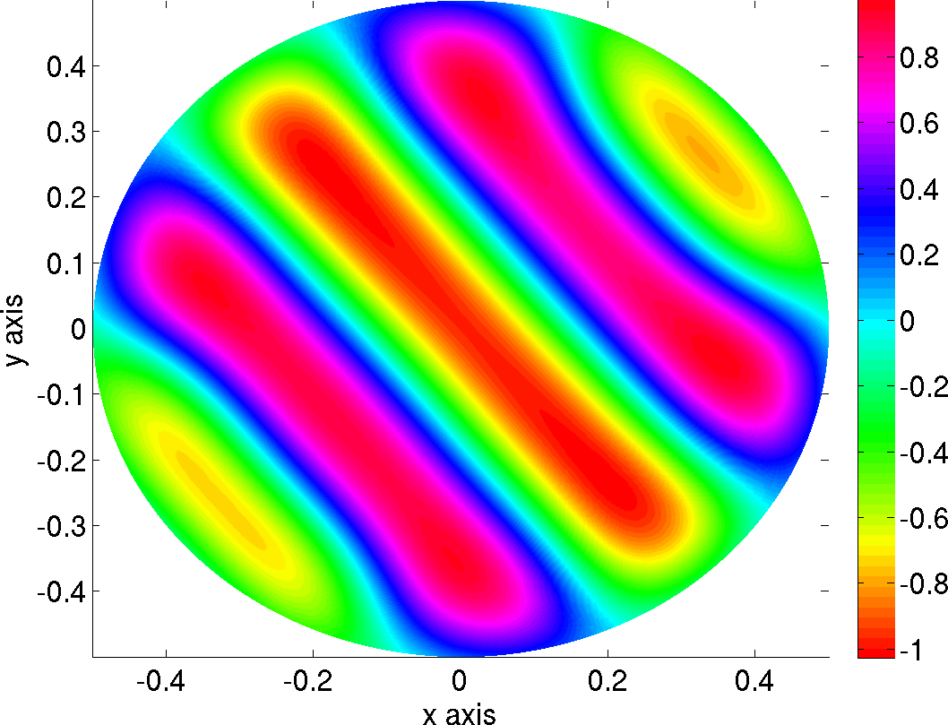
High gain limit
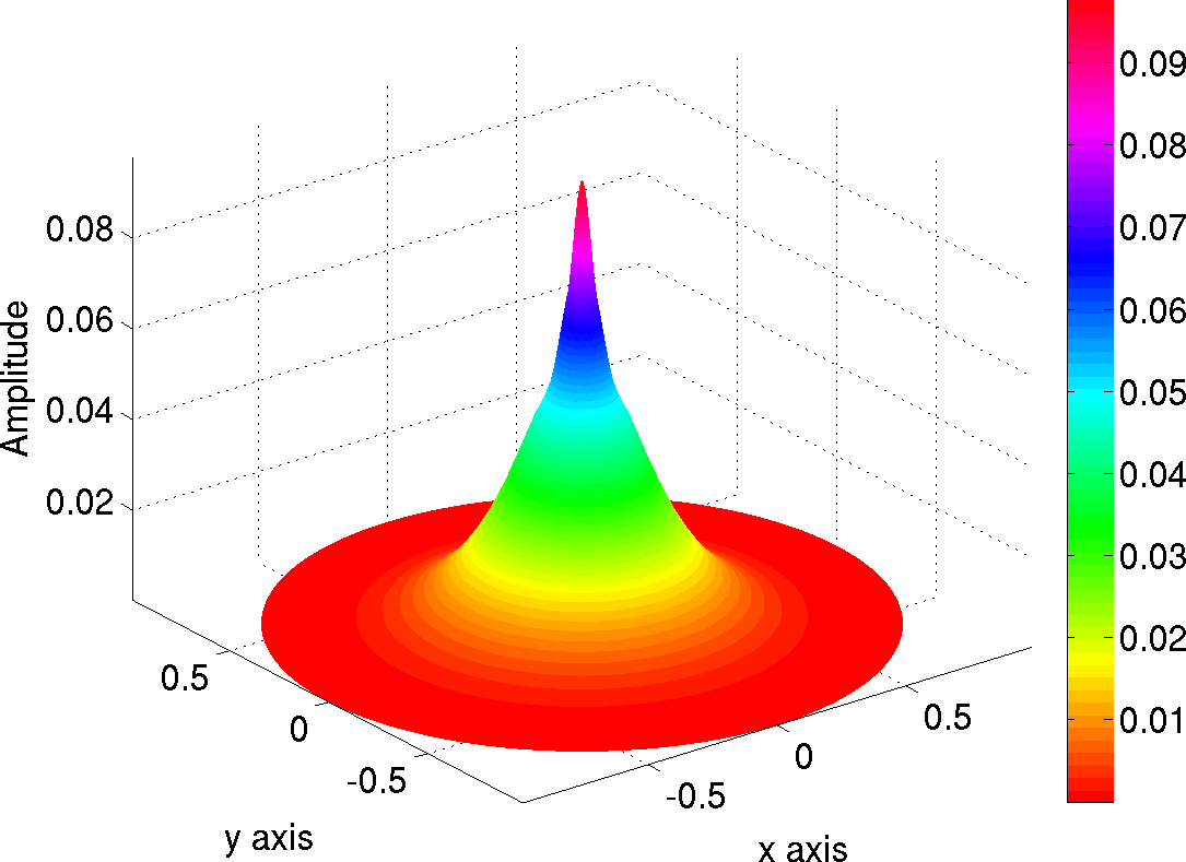
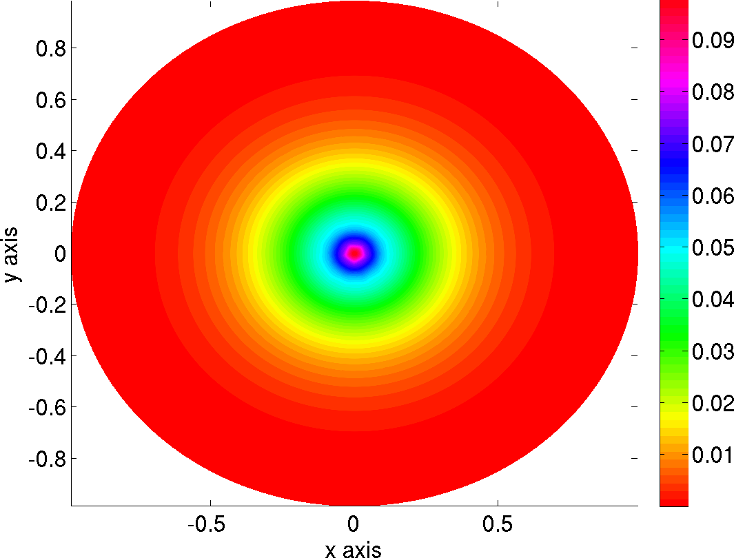
We consider the high gain limit of the sigmoid function and we propose to illustrate section 5 with a numerical simulation. We set , , . We fix the input to be of the form:
with and . Then the condition of existence of a stationary pulse (27) is satisfied, see figure 1. We plot a bump solution according to (27) in figure 4.
6.3 Excitatory and inhibitory connectivity function
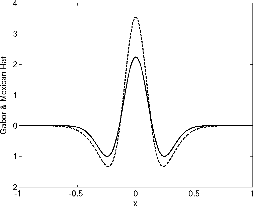
We give some numerical solutions of (7) in the case where the connectivity function is a Gabor function. In all the experiments we set and with . The Gabor function is given by , where is a positive parameter, takes positive values near the origin and negative values further away.
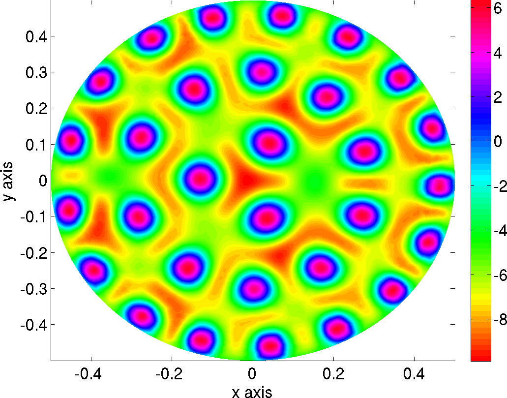
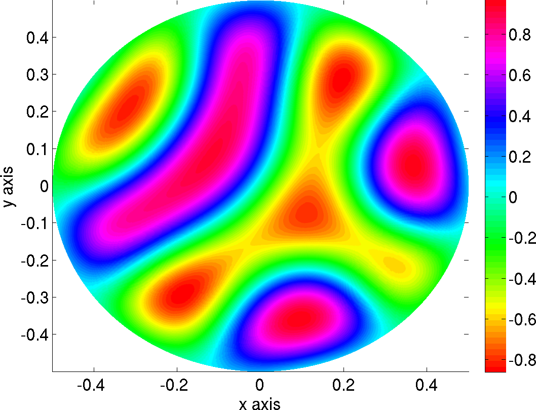
The external input is equal to zero. In figure 5, we show several solutions of equation (7) at for decreasing values of the width of the connectivity. We see the emergence of multi-bump solutions. In figure 5(a), there is one bump centered at . When decreasing the width of the connectivity, for the range of values , the solutions present an increasing number of areas of high level of activity. For example, in figure 5(d), there exist five such areas. Figure 5(e) shows the appearance of a second crown of localized patterns centered at , and figure 5(f) shows three such crowns. Note that all the solutions display interesting symmetries.
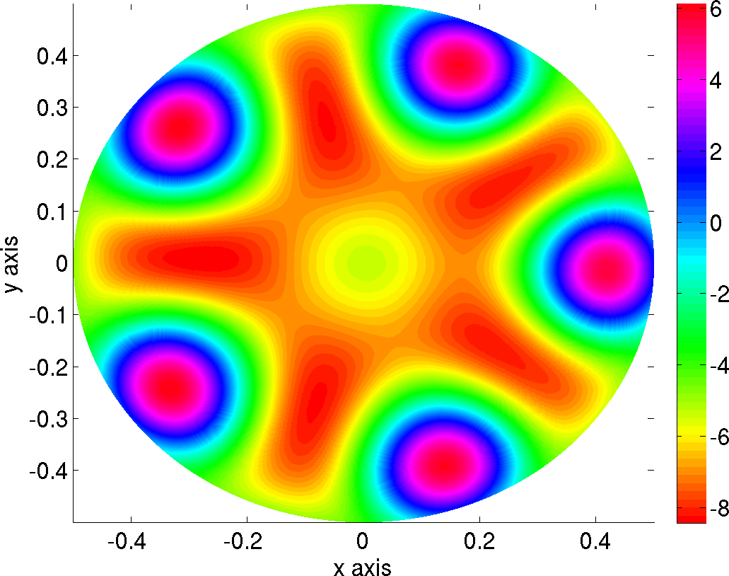
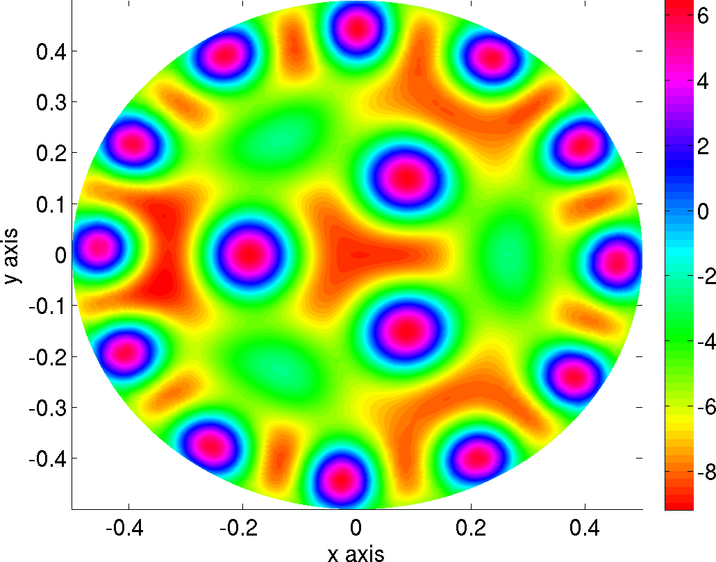
We slightly change the shape of the connectivity function by choosing the difference of two Gaussians . In all the experiments, we take and .
As shown in figure 6 the two connectivity functions, Gabor and difference of Gaussians, feature an excitatory center and an inibitory surround.
We illustrate the behaviour of the solutions when increasing the slope of the sigmoid. We set the sigmoid so that it is equal to 0 at the origin and we choose the external input equal to zero, . In this case the constant function equal to 0 is a solution of (7).
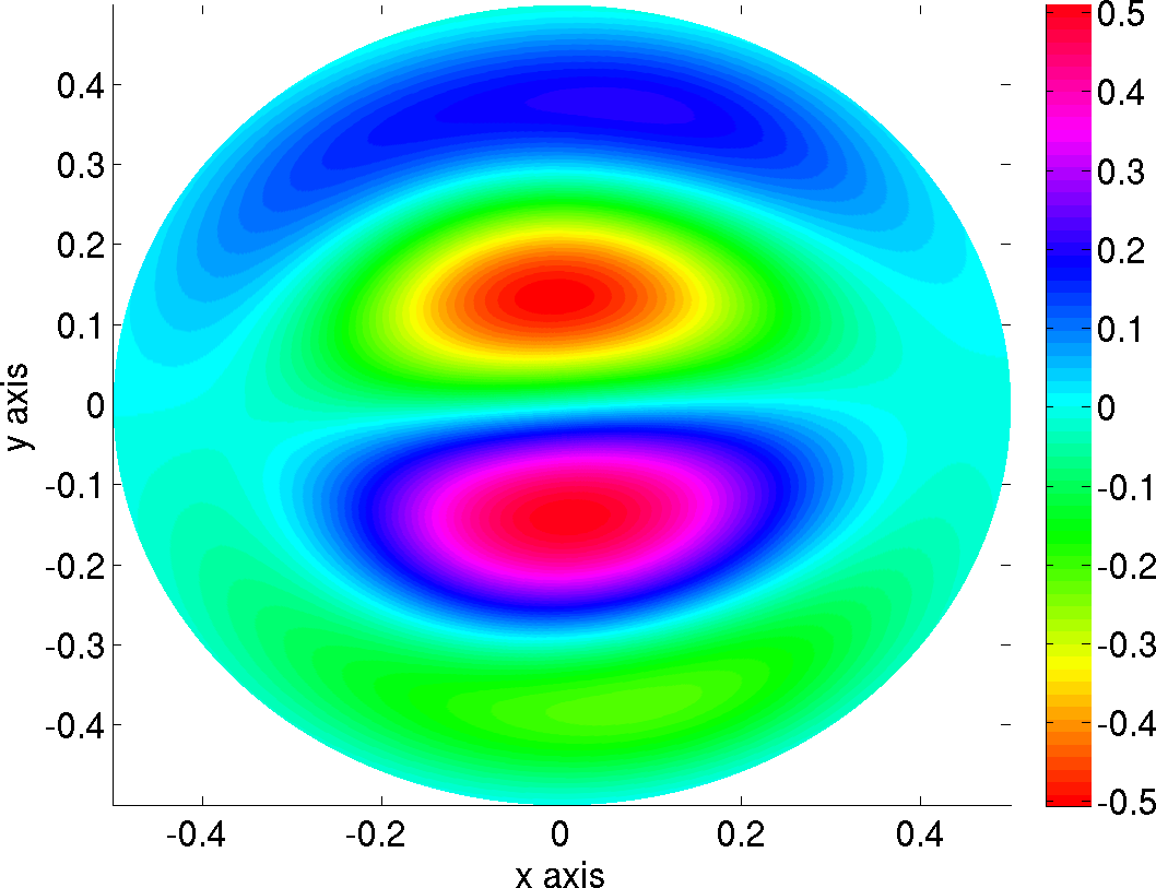
For small values of the slope , the dynamics of the solution is trivial: every solution asymptotically converges to the null solution, as shown in figure 7(a). When increasing , the stability bound, found in subsection 4.5 is no longer satisfied and the null solution may no longer be stable. In effect this solution may bifurcate to other, more interesting solutions. We plot in figures 7(b),7(c),7(d),7(e) and 7(f), some solutions at for different values of . We can see exotic patterns which feature some interesting symmetries. The formal study of these bifurcated solutions is left for future work.
7 Conclusion
We studied the existence and uniqueness of a solution of the equation of a smooth neural field model of structure tensors to model the representation and processing of texture and edges in the visual area V1. We also detailed the analysis of the stationary solutions of this nonlinear integro-differential equation. In both cases functional analysis and the theory of ordinary differential equations have allowed us to introduce the framework in which our equations are well-posed and to begin to characterize their solutions. This is interesting and important in itself but should also be useful for future investigations such as bifurcation analysis.
We have completed our study by constructing and analysing spatially localised bumps in the high-gain limit of the sigmoid function. It is true that networks with Heaviside nonlinearities are not very realistic from the neurobiological perspective and lead to difficult mathematical considerations. However, taking the high-gain limit is instructive since it allows the explicit construction of stationary solutions which is impossible with sigmoidal nonlinearities. We constructed what we called a hyperbolic radially symmetric stationary-pulse and presented a linear stability analysis adapted from [15].
Finally, we illustrated our theoretical results with numerical simulations based on rigorously defined numerical schemes. We hope that our numerical experiments will lead to new and exciting investigations such as a thorough study of the bifurcations of the solutions of our equations with respect to such parameters as the slope of the sigmoid and the width of the connectivity function.
Acknowledgments
This work was partially funded by the ERC advanced grant NerVi number 227747.
Appendix A Volume element in structure tensor space
Let be a structure tensor
its determinant, . can be written
where has determinant 1. Let be the complex number representation of in the Poincaré disk . In this part of the appendix, we present a simple form for the volume element in full structure tensor space, when parametrized as .
Proposition A.0.1.
The volume element in coordinates is
| (32) |
Proof.
In order to compute the volume element in space, we need to express the metric in these coordinates. This is obtained from the inner product in the tangent space at point of . The tangent space is the set of symmetric matrices and the inner product is defined by:
We note that . We note instead of . A basis of (or for that matter) is given by:
and the metric is given by:
The determinant of is equal to , where is the determinant of . is found to be equal to 2. The volume element is thus:
We then use the relations:
where , is given by:
The determinant of the Jacobian of the transformation is found to be equal to:
Hence, the volume element in coordinates is
∎
Appendix B Global existence of solutions
Theorem B.0.1.
Let be an open connected set of a real Banach space and be an open interval of . We consider the initial value problem:
| (33) |
We suppose that and is locally Lipschitz with respect to its second argument. Then for all , there exists and unique solution of (33).
Lemma B.0.1.
Under hypotheses of theorem B.0.1, if and are two solutions and if there exists such that then:
This lemma shows the existence of a larger interval on which the initial value problem (33) has a unique solution. This solution is called the maximal solution.
Theorem B.0.2.
Under hypotheses of theorem B.0.1, let be a maximal solution. We note by the upper bound of and the upper bound of . Then either or for all compact set , there exists such that:
We have the same result with the lower bounds.
Theorem B.0.3.
We suppose and is globally Lipschitz with respect to its second argument. Then for all , there exists a unique solution of (33).
Appendix C Proof of lemma 3.1.2
In this section we prove the following lemma.
Lemma C.0.1.
When is a mexican hat function of and independent of , then:
where erf is the error function defined as:
Proof.
We consider the following double integrals:
| (34) |
so that:
Since the variables are separable, we have:
One can easily see that:
We now give a simplified expression for . We set and then we have, because of lemma 3.1.1:
The change of variable implies and yields:
then we have a simplified expression for :
∎
Appendix D Isometries of
We briefly descrbies the isometries of , i.e the transformations that preserve the distance . We refer to the classical textbooks in hyperbolic goemetry for details, e.g, [20]. The direct isometries (preserving the orientation) in are the elements of the special unitary group, noted , of Hermitian matrices with determinant equal to . Given:
an element of , the corresponding isometry in is defined by:
| (35) |
Orientation reversing isometries of are obtained by composing any transformation (35) with the reflexion . The full symmetry group of the Poincaré disc is therefore:
Let us now describe the different kinds of direct isometries acting in . We first define the following one parameter subgroups of :
Note that and also .
The group is the orthogonal group . Its orbits are concentric circles. It is possible to express each point in hyperbolic polar coordinates: and .
The orbits of converge to the same limit points of the unit circle , when . They are circular arcs in going through the points and .
The orbits of are the circles inside and tangent to the unit circle at . These circles are called horocycles with base point . is called the horocyclic group. It is also possible to express each point in horocyclic coordinates: , where are the transformations associated with the group () and the transformations associated with the subroup ().
Iwasawa decomposition
The following decomposition holds, see [19]:
This theorem allows us to decompose any isometry of as the product of at most thee elements in the groups, and .
References
- [1] S.-I. Amari. Dynamics of pattern formation in lateral-inhibition type neural fields. Biological Cybernetics, 27(2):77–87, jun 1977.
- [2] A. Bellen and M. Zennaro. Numerical Methods for Delay Differential Equations. Oxford Science Publications, 2005.
- [3] R. Ben-Yishai, RL Bar-Or, and H. Sompolinsky. Theory of orientation tuning in visual cortex. Proceedings of the National Academy of Sciences, 92(9):3844–3848, 1995.
- [4] J. Bigun and G. Granlund. Optimal orientation detection of linear symmetry. In Proc. First Int’l Conf. Comput. Vision, pages 433–438. EEE Computer Society Press, 1987.
- [5] P. C. Bressloff and J. D. Cowan. A spherical model for orientation and spatial frequency tuning in a cortical hypercolumn. Philosophical Transactions of the Royal Society B, 2003.
- [6] P.C. Bressloff and J.D. Cowan. SO(3) symmetry breaking mechanism for orientation and spatial frequency tuning in the visual cortex. Phys. Rev. Lett., 88(7), feb 2002.
- [7] P.C. Bressloff and J.D. Cowan. The visual cortex as a crystal. Physica D: Nonlinear Phenomena, 173(3–4):226–258, dec 2002.
- [8] P.C. Bressloff, J.D. Cowan, M. Golubitsky, P.J. Thomas, and M.C. Wiener. Geometric visual hallucinations, Euclidean symmetry and the functional architecture of striate cortex. Phil. Trans. R. Soc. Lond. B, 306(1407):299–330, mar 2001.
- [9] P.C. Bressloff, J.D. Cowan, M. Golubitsky, P.J. Thomas, and M.C. Wiener. What Geometric Visual Hallucinations Tell Us about the Visual Cortex. Neural Computation, 14(3):473–491, 2002.
- [10] M. Camperi and X.J. Wang. A model of visuospatial working memory in prefrontal cortex: Recurrent network and cellular bistability. Journal of Computational Neuroscience, 5:383–405, 1998.
- [11] P. Chossat and O. Faugeras. Hyperbolic planforms in relation to visual edges and textures perception. Plos Computational Biology, 2009. Accepted for publication 11/04/2009.
- [12] Erdelyi. Higher Transcendental Functions, volume 1. Robert E. Krieger Publishing Company, 1985.
- [13] O. Faugeras, R. Veltz, and F. Grimbert. Persistent neural states: stationary localized activity patterns in nonlinear continuous n-population, q-dimensional neural networks. Neural Computation, 21(1):147–187, 2009.
- [14] G. Faye and O. Faugeras. Some theoretical and numerical results for delayed neural field equations. Physica D, 2010. Special issue on Mathematical Neuroscience.
- [15] Stefanos E. Folias and Paul C. Bressloff. Breathing pulses in an excitatory neural network. SIAM Journal on Applied Dynamical Systems, 3(3):378–407, 2004.
- [16] D. Hansel and H. Sompolinsky. Modeling feature selectivity in local cortical circuits. Methods of neuronal modeling, pages 499–567, 1997.
- [17] S. Helgason. Groups and geometric analysis, volume 83 of Mathematical Surveys and Monographs. American Mathematical Society, 2000.
- [18] E. Hewitt and K. Stromberg. Real and Abstract Analysis, volume 25. springer-verlag, 1965.
- [19] H. Iwaniec. Spectral methods of automorphic forms, volume 53 of AMS Graduate Series in Mathematics. AMS Bookstore, 2002.
- [20] S. Katok. Fuchsian Groups. Chicago Lectures in Mathematics. The University of Chicago Press, 1992.
- [21] H. Knutsson. Representing local structure using tensors. In Scandinavian Conference on Image Analysis, pages 244–251, 1989.
- [22] Carlo R. Laing and William C. Troy. PDE methods for nonlocal models. SIAM Journal on Applied Dynamical Systems, 2(3):487–516, 2003.
- [23] C.L. Laing, W.C. Troy, B. Gutkin, and G.B. Ermentrout. Multiple bumps in a neuronal model of working memory. SIAM J. Appl. Math., 63(1):62–97, 2002.
- [24] M. Moakher. A differential geometric approach to the geometric mean of symmetric positive-definite matrices. SIAM J. Matrix Anal. Appl., 26(3):735–747, April 2005.
- [25] M.R. Owen, C.R. Laing, and S. Coombes. Bumps and rings in a two-dimensional neural field: splitting and rotational instabilities. New Journal of Physics, 9(10):378–401, 2007.
- [26] H.R. Wilson and J.D. Cowan. Excitatory and inhibitory interactions in localized populations of model neurons. Biophys. J., 12:1–24, 1972.