Experimental Mathematics and Mathematical Physics

Abstract.

One of the most effective techniques of experimental mathematics is to compute mathematical entities such as integrals, series or limits to high precision, then attempt to recognize the resulting numerical values. Recently these techniques have been applied with great success to problems in mathematical physics. Notable among these applications are the identification of some key multi-dimensional integrals that arise in Ising theory, quantum field theory and in magnetic spin theory.

1. Introduction

One of the most effective techniques of experimental mathematics is to compute mathematical entities to high precision, then attempt to recognize the resulting numerical values. Techniques for efficiently performing basic arithmetic operations and transcendental functions to high precision have been known for several decades, and within the past few years these have been extended to definite integrals, sums of infinite series and limits of sequences. Recognition of the resulting numerical values is typically done by calculating a list of $n$ possible terms on the right-hand side of an identity, also to high precision, then applying the pslq algorithm [21, 11] to see if there is a linear relation in this set of $n+1$ values. If pslq does find a credible relation, then by solving this relation for the value in question, one obtains a formula. These techniques have been described in detail in [14], [15], and [9].

In almost applications of this methodology, both in sophistication and in computation time, the most demanding step is the computation of the key value to sufficient precision to permit pslq detection. As we will show below, computation of some high-dimensional integrals, for instance, often requires several hours on a highly parallel computer system. In contrast, applying pslq to find a relation among, say, 20 candidate terms, each computed to 500-digit precision, usually can be done on a single-CPU system in less than a minute.

In our studies of definite integrals, we have used either Gaussian quadrature (in cases where the function is well behaved on a closed interval) or the “tanh-sinh” quadrature scheme due to Takahasi and Mori [29] (in cases where the function has an infinite derivative or blow-up singularity at one or both endpoints). For many integrand functions, these schemes exhibit “quadratic” or “exponential” convergence – dividing the integration interval in half (or, equivalently, doubling the number of evaluation points) approximately doubles the number of correct digits in the result.

The tanh-sinh scheme is based on the observation, rooted in the Euler-Maclaurin summation formula, that for certain bell-shaped integrands (namely those where the function and all higher derivatives rapidly approach zero at the endpoints of the interval), a simple block-function or trapezoidal approximation to the integral is remarkably accurate [3, pg. 180]. This principle is exploited in the tanh-sinh scheme by transforming the integral of a given function $f(x)$ on a finite interval such as $[-1,1]$ to an integral on $(-\infty,\infty)$, by using the change of variable $x=g(t)$, where $g(t)=\tanh(\pi/2\cdot\sinh t)$. The function $g(t)$ has the property that $g(x)\rightarrow 1$ as $x\rightarrow\infty$ and $g(x)\rightarrow-1$ as $x\rightarrow-\infty$, and also that $g^{\prime}(x)$ and all higher derivatives rapidly approach zero for large positive and negative arguments. Thus one can write, for $h>0$,

(1) $$\int_{-1}^{1}f(x)\,{\rm d}x = \int_{-\infty}^{\infty}f(g(t))g^{\prime}(t)\,{\rm d}t\;\approx\;h\sum_{j=-N}^{N}w_{j}f(x_{j}),$$

where the abscissas $x_{j}=g(hj)$, the weights $w_{j}=g^{\prime}(hj)$, and $N$ is chosen large enough that terms beyond $N$ (positive or negative) are smaller than the “epsilon” of the numeric precision being used. In many cases, even where $f(x)$ has an infinite derivative or an integrable singularity at one or both endpoints, the transformed integrand $f(g(t))g^{\prime}(t)$ is a smooth bell-shaped function for which the Euler-Maclaurin argument applies. In these cases, the error in this approximation (1) decreases more rapidly than any fixed power of $h$. Full details are given in [12].

Both Gaussian quadrature and the tanh-sinh scheme are appropriate for analytic functions on a finite interval. Functions on a semi-infinite intervals can be handled by a simple transformation such as:

$$\int_{0}^{\infty}f(t)\,{\rm d}t = \int_{0}^{1}f(t)\,{\rm d}t+\int_{0}^{1}\frac{f(1/t)\,{\rm d}t}{t^{2}}$$

Oscillatory integrands such as $\int_{0}^{\infty}(1/x\sin x)^{p}\,{\rm d}x$ can be efficiently computed by applying a clever technique recently introduced by Ooura and Mori [26]. Let $x=g(t)=Mt/(1-\exp(-2\pi\sinh t))$. Then in the case of $p=2$, for instance,

$$\int_{0}^{\infty}\left(\frac{\sin x}{x}\right)^{2}\,{\rm d}x = \int_{-\infty}^{\infty}\left(\frac{\sin g(t)}{g(t)}\right)^{2}\cdot g^{\prime}(t)\,{\rm d}t$$

$$\approx h\sum_{k=-N}^{N}\left(\frac{\sin g(hk)}{g(hk)}\right)^{2}\cdot g^{\prime}(hk)$$

Now note that if one chooses $M=\pi/h$, then for large $k$, the $g(hk)$ values are all very close to $k\pi$, so the $\sin(g(hk))$ values are all very close to zero. Thus the sum can be truncated after a modest number of terms, as in tanh-sinh quadrature. In practice, this scheme is very effective for oscillatory integrands such as this.

In the next four sections we consider Ising integrals, Bessel moment integrals, ‘box’ integrals, and hyperbolic volumes arising from quantum field theory respectively. We then conclude with a description of very recent work on multidimensional sums: Euler sums and MZVs.

2. Ising integrals

In a recent study, Bailey, Borwein and Richard Crandall applied tanh-sinh quadrature, implemented using the ARPREC package, to study the following classes of integrals [8]. The $D_{n}$ integrals arise in the Ising theory of mathematical physics, and the $C_{n}$ have tight connections to quantum field theory.

$$C_{n} = \frac{4}{n!}\int_{0}^{\infty}\cdots\int_{0}^{\infty}\frac{1}{\left(\sum_{j=1}^{n}(u_{j}+1/u_{j})\right)^{2}}\frac{{\rm d}u_{1}}{u_{1}}\cdots\frac{{\rm d}u_{n}}{u_{n}}$$

$$D_{n} = \frac{4}{n!}\int_{0}^{\infty}\cdots\int_{0}^{\infty}\frac{\prod_{i<j}\left(\frac{u_{i}-u_{j}}{u_{i}+u_{j}}\right)^{2}}{\left(\sum_{j=1}^{n}(u_{j}+1/u_{j})\right)^{2}}\frac{{\rm d}u_{1}}{u_{1}}\cdots\frac{{\rm d}u_{n}}{u_{n}}$$

$$E_{n} = 2\int_{0}^{1}\cdots\int_{0}^{1}\left(\prod_{1\leq j<k\leq n}\frac{u_{k}-u_{j}}{u_{k}+u_{j}}\right)^{2}{\rm d}t_{2}\,{\rm d}t_{3}\cdots dt_{n},$$

where (in the last line) $u_{k}=\prod_{i=1}^{k}t_{i}$.

Needless to say, evaluating these $n$-dimensional integrals to high precision presents a daunting computational challenge. Fortunately, in the first case, we were able to show that the $C_{n}$ integrals can be written as one-dimensional integrals:

$$C_{n} = \frac{2^{n}}{n!}\int_{0}^{\infty}pK_{0}^{n}(p)\,{\rm d}p,$$

where $K_{0}$ is the modified Bessel function [1]. After computing $C_{n}$ to 1000-digit accuracy for various $n$, we were able to identify the first few instances of $C_{n}$ in terms of well-known constants, e.g.,

$$C_{3} = {\rm L}_{-3}(2)\;=\;\sum_{n\geq 0}\left(\frac{1}{(3n+1)^{2}}-\frac{1}{(3n+2)^{2}}\right)$$

$$C_{4} = \frac{7}{12}\zeta(3),$$

where $\zeta$ denotes the Riemann zeta function. When we computed $C_{n}$ for fairly large $n$, for instance

$$C_{1024} = 0.63047350337438679612204019271087890435458707871273234\dots,$$

we found that these values rather quickly approached a limit. By using the new edition of the Inverse Symbolic Calculator, available at http://ddrive.cs.dal.ca/~isc, this numerical value can be identified as

$$\lim_{n\rightarrow\infty}C_{n} = 2e^{-2\gamma},$$

where $\gamma$ is Euler’s constant. We later were able to prove this fact—this is merely the first term of an asymptotic expansion—and thus showed that the $C_{n}$ integrals are fundamental in this context [8].

The integrals $D_{n}$ and $E_{n}$ are much more difficult to evaluate, since they are not reducible to one-dimensional integrals (as far as we can tell), but with certain symmetry transformations and symbolic integration we were able to reduce the dimension in each case by one or two. In the case of $D_{5}$ and $E_{5}$, the resulting 3-D integrals are extremely complicated, but we were nonetheless able to numerically evaluate these to at least 240-digit precision on a highly parallel computer system. In this way, we produced the following evaluations, all of which except the last we subsequently were able to prove:

$$D_{2} = 1/3$$

$$D_{3} = 8+4\pi^{2}/3-27\,{\rm L}_{-3}(2)$$

$$D_{4} = 4\pi^{2}/9-1/6-7\zeta(3)/2$$

$$E_{2} = 6-8\log 2$$

$$E_{3} = 10-2\pi^{2}-8\log 2+32\log^{2}2$$

$$E_{4} = 22-82\zeta(3)-24\log 2+176\log^{2}2-256(\log^{3}2)/3+16\pi^{2}\log 2-22\pi^{2}/3$$

$$E_{5} \stackrel{{\scriptstyle?}}{{=}} 42-1984\,{\rm Li}_{4}(1/2)+189\pi^{4}/10-74\zeta(3)-1272\zeta(3)\log 2+40\pi^{2}\log^{2}2$$

$$-62\pi^{2}/3+40(\pi^{2}\log 2)/3+88\log^{4}2+464\log^{2}2-40\log 2,$$

where ${\rm Li}$ denotes the polylogarithm function. In the case of $D_{2},\,D_{3}$ and $D_{4}$, these are confirmations of known results. We tried but failed to recognize $D_{5}$ in terms of similar constants (the 500-digit numerical value is available if anyone wishes to try). The conjectured identity shown here for $E_{5}$ was confirmed to 240-digit accuracy, which is 180 digits beyond the level that could reasonably be ascribed to numerical round-off error; thus we are quite confident in this result even though we do not have a formal proof.

In a follow-on study [6], we examined the following generalization of the $C_{n}$ integrals:

$$C_{n,k} = \frac{4}{n!}\,\int_{0}^{\infty}\cdots\int_{0}^{\infty}\frac{1}{\left(\sum_{j=1}^{n}(u_{j}+1/u_{j})\right)^{k+1}}\frac{{\rm d}u_{1}}{u_{1}}\cdots\frac{{\rm d}u_{n}}{u_{n}}.$$

Here we made the initially surprising discovery—now proven in [17] and in outline much earlier [13]—that there are linear relations in each of the rows of this array (considered as a doubly-infinite rectangular matrix), e.g.,

$$0 = C_{3,0}-84C_{3,2}+216C_{3,4}$$

$$0 = 2C_{3,1}-69C_{3,3}+135C_{3,5}$$

$$0 = C_{3,2}-24C_{3,4}+40C_{3,6}$$

$$0 = 32C_{3,3}-630C_{3,5}+945C_{3,7}$$

$$0 = 125C_{3,4}-2172C_{3,6}+3024C_{3,8}.$$

3. Bessel moment integrals

In a more recent study of Bessel moment integrals, co-authored with Larry Glasser [7], the first three authors were able to analytically recognize many of the $C_{n,k}$ constants in the earlier study—because, remarkably, these same integrals appear naturally in quantum field theory (for odd $k$). We also discovered, and then proved with considerable effort, that with $c_{n,k}$ normalized by $C_{n,k}={2^{n}}\,c_{n,k}/(n!\,k!)$, we have

$$c_{3,0} = \frac{3\Gamma^{6}(1/3)}{32\pi 2^{2/3}}\;=\;\frac{\sqrt{3}\pi^{3}}{8}{}_{3}F_{2}\left(\begin{array}[]{c}1/2,1/2,1/2\\ 1,1\end{array}\Bigg{|}\frac{1}{4}\right)$$

$$c_{3,2} = \frac{\sqrt{3}\pi^{3}}{288}{}_{3}F_{2}\left(\begin{array}[]{c}1/2,1/2,1/2\\ 2,2\end{array}\Bigg{|}\frac{1}{4}\right)$$

$$c_{4,0} = \frac{\pi^{4}}{4}\sum_{n=0}^{\infty}\frac{{2n\choose n}^{4}}{4^{4n}}\;=\;\frac{\pi^{4}}{4}{}_{4}F_{3}\left(\begin{array}[]{c}1/2,1/2,1/2,1/2\\ 1,1,1\end{array}\Bigg{|}1\right)$$

$$c_{4,2} = \frac{\pi^{4}}{64}\left[4\,{}_{4}F_{3}\left(\begin{array}[]{c}1/2,1/2,1/2,1/2\\ 1,1,1\end{array}\Bigg{|}1\right)\right.$$

$$\left.-3\,{}_{4}F_{3}\left(\begin{array}[]{c}1/2,1/2,1/2,1/2\\ 2,1,1\end{array}\Bigg{|}1\right)\right]-\frac{3\pi^{2}}{16},$$

where ${}_{p}F_{q}$ denotes the generalized hypergeometric function [1]. The corresponding values for small odd second indices are $c_{3,1}=3L_{-3}(2)/4,\,c_{3,3}=L_{-3}(2)-2/3,\,c_{4,1}=7\zeta(3)/8$ and $c_{4,3}=7\zeta(3)/32-3/16$.

Integrals in the Bessel moment study were quite challenging to evaluate numerically. As one example, we sought to numerically verify the following identity that we had derived analytically:

$$c_{5,0} = \frac{\pi}{2}\int_{-\pi/2}^{\pi/2}\int_{-\pi/2}^{\pi/2}\frac{{\bf K}(\sin\theta)\,{\bf K}(\sin\phi)}{\sqrt{\cos^{2}\theta\cos^{2}\phi+4\sin^{2}(\theta+\phi)}}\,{\rm d}\theta\,{\rm d}\phi\,,$$

where ${\bf K}$ denotes the elliptic integral of the first kind [1]. Note that this function has blow-up singularities on all four sides of the region of integration, with particularly troublesome singularities at $(\pi/2,-\pi/2)$ and $(-\pi/2,\pi/2)$ (see Figure 1). Nonetheless, after making some minor substitutions, we were able to evaluate (and confirm) this integral to 120-digit accuracy (using 240-digit working precision) in a run of 43 minutes on 1024 cores of the “Franklin” system at LBNL.

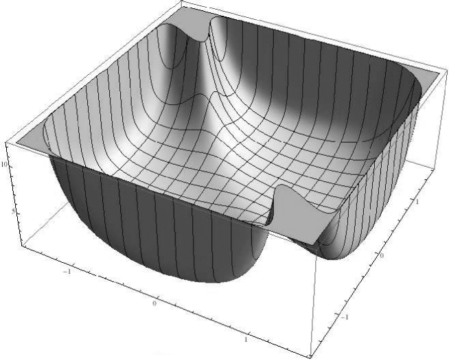
Figure 1. Plot of $c_{5,0}$ integrand function

In a separate study, the first two authors studied correlation integrals for the Heisenberg spin-1/2 antiferromagnet, as given by Boos and Korepin, for a length-$n$ spin chain [24, eqn. 2.2]:

$$P(n) := \frac{\pi^{n(n+1)/2}}{(2\pi i)^{n}}\cdot\int_{-\infty}^{\infty}\int_{-\infty}^{\infty}\cdots\int_{-\infty}^{\infty}U(x_{1}-i/2,x_{2}-i/2,\cdots,x_{n}-i/2)$$

$$\times\;T(x_{1}-i/2,x_{2}-i/2,\cdots,x_{n}-i/2)\,{\rm d}x_{1}\,{\rm d}x_{2}\cdots{\rm d}x_{n}$$

where

$$U(x_{1}-i/2,x_{2}-i/2,\cdots,x_{n}-i/2) = \frac{\prod_{1\leq k<j\leq n}\sinh[\pi(x_{j}-x_{k})]}{\prod_{1\leq j\leq n}i^{n}\cosh^{n}(\pi x_{j})}$$

$$T(x_{1}-i/2,x_{2}-i/2,\cdots,x_{n}-i/2) = \frac{\prod_{1\leq j\leq n}(x_{j}-i/2)^{j-1}(x_{j}+i/2)^{n-j}}{\prod_{1\leq k<j\leq n}(x_{j}-x_{k}-i)}.\hskip 10.00002pt$$

They computed numerical values for these $n$-fold integrals to as great a precision as we could, then attempted to recognize them using pslq. They found the following, which confirm some earlier results obtained by others using physical symmetry methods:

$$P(1) = \frac{1}{2}$$

$$P(2) = \frac{1}{3}-\frac{1}{3}\log 2$$

$$P(3) = \frac{1}{4}-\log 2+\frac{3}{8}\zeta(3)$$

$$P(4) = \frac{1}{5}-2\log 2+\frac{173}{60}\zeta(3)-\frac{11}{6}\zeta(3)\log 2-\frac{51}{80}\zeta^{2}(3)-\frac{55}{24}\zeta(5)+\frac{85}{24}\zeta(5)\log 2$$

$$P(5) = \frac{1}{6}-\frac{10}{3}\log 2+\frac{281}{24}\zeta(3)-\frac{45}{2}\zeta(3)\log 2-\frac{489}{16}\zeta^{2}(3)-\frac{6775}{192}\zeta(5)$$

$$+\frac{1225}{6}\zeta(5)\log 2-\frac{425}{64}\zeta(3)\zeta(5)-\frac{12125}{256}\zeta^{2}(5)+\frac{6223}{256}\zeta(7)$$

$$-\frac{11515}{64}\zeta(7)\log 2+\frac{42777}{512}\zeta(3)\zeta(7)$$

$n$	Digits	Processors	Run Time
2	120	1	10 sec.
3	120	8	55 min.
4	60	64	27 min.
5	30	256	39 min.
6	6	256	59 hrs.

Table 1. Run times and precision levels for spin integral calculations

These computations underscore the rapidly increasing cost of computing integrals in higher dimensions. Precision levels, processor counts and run times are shown in Table 1.

4. Box integrals

Let us define box integrals for dimension $n$ as

$$B_{n}(s) := \int_{0}^{1}\cdots\int_{0}^{1}\left(r_{1}^{2}+\dots+r_{n}^{2}\right)^{s/2}\,{\rm d}r_{1}\cdots{\rm d}r_{n}$$

$$\Delta_{n}(s) := \int_{0}^{1}\cdots\int_{0}^{1}\left((r_{1}-q_{1})^{2}+\dots+(r_{n}-q_{n})^{2}\right)^{s/2}\,{\rm d}r_{1}\cdots{\rm d}r_{n}\,{\rm d}q_{1}\cdots{\rm d}q_{n}.$$

As explained in previous treatments [4, 5], these integrals have several physical interpretations:

1. $B_{n}(1)$ is the expected distance of a random point from the origin (or from any fixed vertex) of the $n$-cube.

2. $\Delta_{n}(1)$ is the expected distance between two random points of the $n$-cube.

3. $B_{n}(-n+2)$ is the expected electrostatic potential in an $n$-cube whose origin has a unit charge. Such statements presume that electrostatic potential in $n$ dimensions is $V(r)=1/r^{n-2}$, and say $\log r$ for $n=2$; in other words, the negative powers of $r$ can also have physical meaning.

4. $\Delta_{n}(-n+2)$ is the expected electrostatic energy between two points in a uniform cube of charged “jellium.”

5. Recently integrals of this type have arisen in neuroscience e.g., the average distance between synapses in a mouse brain.

Note that the definitions show immediately that both $\Delta_{n}(2m)$ and $B_{n}(2m)$ are rational when $m,n$ are natural numbers. A pivotal, original treatment on box integrals is the 1976 work of Anderssen et al [2]. There have been interesting modern treatments of the $B_{n}$ and related integrals, as in [10], [14, pg. 208], [32], and [30]. Related material may also be found in [23, 31].

Like the Ising integrals, some of these $n$-dimensional integrals are reducible to 1-dimension integrals. For instance, we found that

$$\Delta_{3}(-1) = \frac{2}{\sqrt{\pi}}\int_{0}^{\infty}\frac{(-1+e^{-u^{2}}+\sqrt{\pi}\,u\,{\rm erf}(u))^{3}}{u^{6}}\,{\rm d}u.$$

After calculating a 400-digit numerical value for this constant, we were able to recognize it as

$$\Delta_{3}(-1) = \frac{1}{15}\left(6+6\sqrt{2}-12\sqrt{3}-10\pi+30\log(1+\sqrt{2})+30\log(2+\sqrt{3})\right).$$

$n$	$s$	$B_{n}(s)$
any	even $s\geq 0$	rational, e.g.: $B_{2}(2)=2/3$
1	$s\neq-1$	$\frac{1}{s+1}$
2	$-4$	$-\frac{1}{4}-\frac{\pi}{8}$
2	$-3$	$-\sqrt{2}$
2	$-1$	$2\log(1+\sqrt{2})$
2	1	$\frac{1}{3}\sqrt{2}+\frac{1}{3}\log(1+\sqrt{2})$
2	3	$\frac{7}{20}\sqrt{2}+\frac{3}{20}\log(1+\sqrt{2})$
2	$s\neq-2$	$\frac{2}{2+s}\,{}_{2}F_{1}\left(\frac{1}{2},-\frac{s}{2};\frac{3}{2};-1\right)$
3	$-5$	$-\frac{1}{6}\sqrt{3}-\frac{1}{12}\pi$
3	$-4$	$-\frac{3}{2}\sqrt{2}\arctan\frac{1}{\sqrt{2}}$
3	$-2$	$-3G+\frac{3}{2}\pi\log(1+\sqrt{2})+3\,{\rm Ti}_{2}(3-2\sqrt{2})$
3	$-1$	$-\frac{1}{4}\pi+\frac{3}{2}\log\left(2+\sqrt{3}\right)$
3	1	$\frac{1}{4}\sqrt{3}-\frac{1}{24}\pi+\frac{1}{2}\log\left(2+\sqrt{3}\right)$
3	3	$\frac{2}{5}\sqrt{3}-\frac{1}{60}\pi+\frac{7}{20}\log\left(2+\sqrt{3}\right)$

Table 2. Recent evaluations of Box integrals

$n$	$s$	$B_{n}(s)$
4	$-5$	$-\sqrt{8}\,\arctan\left(\frac{1}{\sqrt{8}}\right)$
4	$-3$	$4\ G-12\,{\rm Ti}_{2}(3-2\sqrt{2})$
4	$-2$	$\pi\,\log\left(2+\sqrt{3}\right)-2\,G-\frac{\pi^{2}}{8}$
4	$-1$	$2\log 3-\frac{2}{3}\,G+2\,{\rm Ti_{2}}\left(3-2\,\sqrt{2}\right)-\sqrt{8}\,\arctan\left(\frac{1}{\sqrt{8}}\right)$
4	1	$\frac{2}{5}-\frac{G}{10}+\frac{3}{10}\,{\rm Ti_{2}}\left(3-2\sqrt{2}\right)+\log 3-\frac{7\sqrt{2}}{10}\,\arctan\left(\frac{1}{\sqrt{8}}\right)$
5	$-3$	${\frac{110}{9}}\,G-10\,\log\left(2-\sqrt{3}\right)\,\theta-\frac{1}{8}\,{\pi}^{2}$
		$-10\,{\rm Cl}_{2}\left(\frac{1}{3}\,\theta+\frac{1}{3}\,\pi\right)+10\,{\rm Cl}_{2}\left(\frac{1}{3}\,\theta-\frac{1}{6}\,\pi\right)+\frac{10}{3}\,{\rm Cl}_{2}\left(\theta+\frac{1}{6}\,\pi\right)$
		$+{\frac{20}{3}}\,{\rm Cl}_{2}\left(\theta+\frac{4}{3}\,\pi\right)-{\frac{10}{3}}\,{\rm Cl}_{2}\left(\theta+\frac{5}{3}\,\pi\right)-{\frac{20}{3}}\,{\rm Cl}_{2}\left(\theta+{\frac{11}{6}}\,\pi\right)$
5	$-2$	$\frac{8}{3}\,B_{5}(-6)-\frac{1}{3}\,B_{5}(-4)+\frac{5}{2}\,\pi\log 3+10\,{\rm Ti}_{2}\left(\frac{1}{3}\right)-10\,G$
5	$-1$	$-{\frac{110}{27}}\,G+\frac{10}{3}\,\theta\log\left(2-\sqrt{3}\right)+\frac{1}{48}\,{\pi}^{2}$
		$+5\,\log\left(\frac{1+\sqrt{5}}{2}\right)-\frac{5}{2}\,\sqrt{3}\arctan\left(\frac{1}{\sqrt{15}}\right)$
		$+\frac{10}{3}\,{\rm Cl}_{2}\left(\frac{1}{3}\,\theta+\frac{1}{3}\,\pi\right)-\frac{10}{3}\,{\rm Cl}_{2}\left(\frac{1}{3}\,\theta-\frac{1}{6}\,\pi\right)-\frac{10}{9}\,{\rm Cl}_{2}\left(\theta+\frac{1}{6}\,\pi\right)$
		$-{\frac{20}{9}}\,{\rm Cl}_{2}\left(\theta+\frac{4}{3}\,\pi\right)+{\frac{10}{9}}\,{\rm Cl}_{2}\left(\theta+\frac{5}{3}\,\pi\right)+{\frac{20}{9}}\,{\rm Cl}_{2}\left(\theta+{\frac{11}{6}}\,\pi\right)$
5	1	$-\frac{77}{81}\,G+\frac{7}{9}\,\theta\log\left(2-\sqrt{3}\right)+\frac{1}{360}\,{\pi}^{2}+\frac{1}{6}\,\sqrt{5}$
		$+\frac{10}{3}\,\log\left(\frac{1+\sqrt{5}}{2}\right)-\frac{4}{3}\,\sqrt{3}\arctan\left(\frac{1}{\sqrt{15}}\right)$
		$+{\frac{7}{9}}\,{\rm Cl}_{2}\left(\frac{1}{3}\,\theta+\frac{1}{3}\,\pi\right)-\frac{7}{9}\,{\rm Cl}_{2}\left(\frac{1}{3}\,\theta-\frac{1}{6}\,\pi\right)-{\frac{7}{27}}\,{\rm Cl}_{2}\left(\theta+\frac{1}{6}\,\pi\right)$
		$-{\frac{14}{27}}\,{\rm Cl}_{2}\left(\theta+\frac{4}{3}\,\pi\right)+{\frac{7}{27}}\,{\rm Cl}_{2}\left(\theta+\frac{5}{3}\,\pi\right)+{\frac{14}{27}}\,{\rm Cl}_{2}\left({\theta+\frac{11}{6}}\,\pi\right)$

Table 3. Recent evaluations of Box integrals, continued; here $\theta:={\rm arctan}\left(\frac{16-3\sqrt{15}}{11}\right)$

$n$	$s$	$\Delta_{n}(s)$
2	$-5$	$\frac{4}{3}+\frac{8}{9}\sqrt{2}$
2	$-1$	$\frac{4}{3}-\frac{4}{3}\sqrt{2}+4\log(1+\sqrt{2})$
2	1	$\frac{2}{15}+\frac{1}{15}\sqrt{2}+\frac{1}{3}\log(1+\sqrt{2})$
3	$-7$	$\frac{4}{5}-\frac{16\sqrt{2}}{15}+\frac{2\sqrt{3}}{5}+\frac{\pi}{15}$
3	$-2$	$2\pi-12\ G+12\,{\rm Ti}_{2}\left(3-2\sqrt{2}\right)+6\pi\log\left(1+\sqrt{2}\right)$
		$+2\log 2-\frac{5}{2}\log 3-8\sqrt{2}\arctan\left(\frac{1}{\sqrt{2}}\right)$
3	$-1$	$\frac{2}{5}-\frac{2}{3}\pi+\frac{2}{5}\sqrt{2}-\frac{4}{5}\sqrt{3}+2\log\left(1+\sqrt{2}\right)+12\log\left(\frac{1+\sqrt{3}}{\sqrt{2}}\right)-4\log\left(2+\sqrt{3}\right)$
3	1	$-{\frac{118}{21}}-\frac{2}{3}\,\pi+{\frac{34}{21}}\,\sqrt{2}-\frac{4}{7}\,\sqrt{3}+2\,\log\left(1+\sqrt{2}\right)+8\,\log\left(\frac{1+\sqrt{3}}{\sqrt{2}}\right)$
3	3	$-{\frac{1}{105}}-{\frac{2}{105}}\,\pi+{\frac{73}{840}}\,\sqrt{2}+\frac{1}{35}\,\sqrt{3}+{\frac{3}{56}}\,\log\left(1+\sqrt{2}\right)+{\frac{13}{35}}\,\log\left(\frac{1+\sqrt{3}}{\sqrt{2}}\right)$

Table 4. Recent evaluations of Box integrals, continued

$n$	$s$	$\Delta_{n}(s)$
4	$-3$	$-{\frac{128}{15}}+\frac{16}{3}\,\pi-8\,\log\left(1+\sqrt{2}\right)-32\,\log\left(1+\sqrt{3}\right)+16\,\log 2+20\,\log 3$
		$-\frac{8}{5}\,\sqrt{2}+{\frac{32}{5}}\,\sqrt{3}-32\,\sqrt{2}\arctan\left(\frac{1}{\sqrt{8}}\right)-96\,{\rm Ti}_{2}\left(3-2\,\sqrt{2}\right)+32\,{G}$
4	$-2$	$-{\frac{16}{15}}\,\pi\,\sqrt{3}-\frac{8}{3}\,\pi\,\log 2+\frac{16}{3}\,\pi\,\log\left(1+\sqrt{3}\right)-\frac{2}{3}\,{\pi}^{2}+\frac{4}{5}\,\pi$
		$+\frac{8}{5}\,\sqrt{2}\arctan\left(2\,\sqrt{2}\right)+\frac{2}{5}\,\log 3-4\,\pi\,\log\left(\sqrt{2}-1\right)$
		$+8{\rm Ti}_{2}\left(3-2\,\sqrt{2}\right)-{\frac{40}{3}}G-\frac{8}{3}\,\log 2$
4	$-1$	$-{\frac{152}{315}}-{\frac{8}{15}}\,\pi-{\frac{16}{5}}\,\log 2+\frac{2}{5}\,\log 3+{\frac{68}{105}}\,\sqrt{2}-{\frac{16}{35}}\,\sqrt{3}+\frac{4}{5}\,\log\left(1+\sqrt{2}\right)$
		$+{\frac{32}{5}}\,\log\left(1+\sqrt{3}\right)-\frac{8}{3}\,G+8{\rm Ti}_{2}\left(3-2\,\sqrt{2}\right)-\frac{8}{5}\,\sqrt{2}\arctan\left(\sqrt{2}/4\right)$
4	1	$-{\frac{23}{135}}-{\frac{16}{315}}\,\pi-{\frac{52}{105}}\,\log 2+{\frac{197}{420}}\,\log 3+{\frac{73}{630}}\,\sqrt{2}+{\frac{8}{105}}\,\sqrt{3}$
		$+\frac{1}{14}\,\log\left(1+\sqrt{2}\right)+{\frac{104}{105}}\,\log\left(1+\sqrt{3}\right)$
		$-{\frac{68}{105}}\,\sqrt{2}\arctan\left(\frac{1}{\sqrt{8}}\right)-{\frac{4}{15}}\,{G}+\frac{4}{5}\,{\rm Ti}_{2}\left(3-2\,\sqrt{2}\right)$
5	1	$-{\frac{1279}{567}}\,{G}-{\frac{4}{189}}\,\pi+{\frac{4}{315}}\,{\pi}^{2}-{\frac{449}{3465}}+{\frac{3239}{62370}}\,\sqrt{2}+{\frac{568}{3465}}\,\sqrt{3}-{\frac{380}{6237}\,\sqrt{5}}$
		$+{\frac{295}{252}}\,\log 3+{\frac{1}{54}}\,\log\left(1+\sqrt{2}\right)+{\frac{20}{63}}\,\log\left(2+\sqrt{3}\right)+{\frac{64}{189}}\,\log\left(\frac{1+\sqrt{5}}{2}\right)$
		$-{\frac{73}{63}}\,\sqrt{2}\arctan\left(\frac{1}{\sqrt{8}}\right)-{\frac{8}{21}}\,\sqrt{3}\arctan\left(\frac{1}{\sqrt{15}}\right)+{\frac{104}{63}}\,\log\left(2-\sqrt{3}\right)\theta$
		$+\frac{5}{7}\,{\rm Ti}_{2}\left(3-2\,\sqrt{2}\right)+{\frac{104}{63}}\,{\rm Cl_{2}}\left(\frac{1}{3}\,\theta+\frac{1}{3}\,\pi\right)-{\frac{104}{63}}\,{\rm Cl_{2}}\left(\frac{1}{3}\,\theta-\frac{1}{6}\,\pi\right)$
		$-{\frac{104}{189}}\,{\rm Cl_{2}}\left(\theta+\frac{1}{6}\,\pi\right)-{\frac{208}{189}}\,{\rm Cl_{2}}\left(\theta+\frac{4}{3}\,\pi\right)$
		$+{\frac{104}{189}}\,{\rm Cl_{2}}\left(\theta+\frac{5}{3}\,\pi\right)+{\frac{208}{189}}\,{\rm Cl}_{{2}}\left(\theta+{\frac{11}{6}}\,\pi\right)$

Table 5. Recent evaluations of Box integrals, continued

A selection of results that we have found are shown in Tables 2, 3, 4 and 5. Here $G$ denotes Catalan’s constant, namely, $G:=\sum_{n\geq 0}(-1)^{n}/(2n+1)^{2}$, $\theta=\linebreak\arctan\bigl{(}(16-3\sqrt{15})/11\bigr{)}$, Cl denotes Clausen’s function,

$${\rm Cl}_{2}(\theta) = \sum_{n\geq 1}\frac{\sin(n\theta)}{n^{2}},$$

and Ti denotes Lewin’s inverse-tan function,

$${\rm Ti_{2}}(x) = \sum_{n\geq 0}(-1)^{n}\frac{x^{2n+1}}{(2n+1)^{2}}.$$

5. Clausen functions and hyperbolic volumes

In an unpublished 1998 study [16] two of the present authors (Borwein and Broadhurst) identified 998 closed hyperbolic 3-manifolds whose volumes are rationally related to Dedekind zeta values, with coprime integers $a$ and $b$ giving

(7) $$\frac{a}{b}\,{\rm vol}({\mathcal{M}}) = \frac{(-D)^{3/2}}{(2\pi)^{2n-4}}\,\frac{\zeta_{K}(2)}{2\zeta(2)}$$

for a manifold ${\mathcal{M}}$ whose invariant trace field $K$ has a single complex place, discriminant $D$, degree $n$, and Dedekind zeta value $\zeta_{K}(2)$. While the existence of integers $a,b$ can be established, via algebraic $K$-theory as in [35], for the most part it was and is not possible to specify the rational $a/b$ other than empirically [35].

The simplest identity implicit in (7) devolves to

(8) $$3\,{\rm Cl}_{2}(\alpha)-\,3{\rm Cl}_{2}(2\alpha)+{\rm Cl}_{2}(3\alpha) = \frac{7\sqrt{7}}{4}\,{\rm L}_{-7}(2),$$

with $\alpha=2\arctan(\sqrt{7}),$ as is recorded in [14, p. 91]. Here $L_{-7}(2):=\sum_{n>0}\left(\frac{n}{7}\right)/n^{2}$ is the primitive Dirichlet $L$-series modulo 7 evaluated at 2 where $\left(\frac{n}{7}\right)$ is the Legendre symbol. This was rewritten in equivalent and more self-contained form as

(9) $$\frac{24}{7\sqrt{7}}\,\int_{\pi/3}^{\pi/2}\,\log\left|\frac{\tan t+\sqrt{7}}{\tan t-\sqrt{7}}\right|\,{{\mathrm{d}}t} = {\rm L}_{-7}(2)$$

in [9, p. 61]—and elsewhere.

Note that the integrand function of (9) has a nasty singularity at $\arctan(\sqrt{7})$ (see Figure 2). However, we were able to numerically evaluate this integral to 20,000-digit accuracy, by splitting the integral into two parts, namely on the intervals $[\pi/3,\arctan(\sqrt{7})]$ and $[\arctan(\sqrt{7}),\pi/2]$. Note that tanh-sinh quadrature can be used on each part, since it can readily handle blow-up singularities at one or both endpoints of the interval of integration. This run required 46 minutes on 1024 CPUs of the Virginia Tech Apple cluster. The right-hand side was also evaluated, using Mathematica, to 20,000-digit precision. The two values agreed to $19,995$ digits [9, pg. 61]. Alternative representations of the integral in (9) are given in [20].

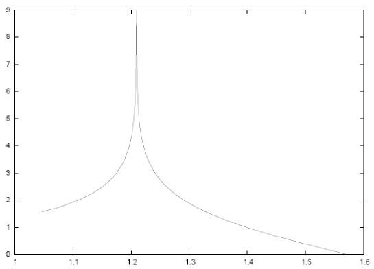
Figure 2. Plot of integrand function in (9)

We shall now provide a proof of Eqn. (8) and hence of Eqn. (9). Actually, an equivalent (if not obviously so) form of identity (8), namely

$$\zeta_{\mathbb{Q}(\sqrt{-7})}(2) = \frac{\pi^{2}}{3\sqrt{7}}\Bigl{\{}A\Bigl{(}\cot\frac{\pi}{7}\Bigr{)}+A\Bigl{(}\cot\frac{2\pi}{7}\Bigr{)}+A\Bigl{(}\cot\frac{4\pi}{7}\Bigr{)}\Bigr{\}}$$

$$= \frac{2\pi^{2}}{7\sqrt{7}}\bigl{\{}2A(\sqrt{7})+A(\sqrt{7}+2\sqrt{3})+A(\sqrt{7}-2\sqrt{3})\bigr{\}}$$

with the notation

$$A(x) := \int_{0}^{x}\frac{1}{1+t^{2}}\,\log\frac{4}{1+t^{2}}\,{\mathrm{d}}t\;=\;{\rm Cl}_{2}(2\operatorname{arccot}x),$$

is already established in [33]. The first equality in (5) can be written as

(11) $$\zeta_{\mathbb{Q}(\sqrt{-7})}(2) = \frac{\pi^{2}}{6}\,{\rm L}_{-7}(2)\quad\;=\;\quad\zeta(2)\,{\rm L}_{-7}(2).$$

On noting that

$$\cot\arg\frac{\sqrt{7}+i}{2\sqrt{2}} = \sqrt{7}$$

$$\cot\arg\frac{(1+i\sqrt{7})(1\mp i\sqrt{3})}{4\sqrt{2}} = \sqrt{7}\pm 2\sqrt{3}$$

$${\rm Cl}_{2}(\theta) = \operatorname{Im}\sum_{n\geq 1}\frac{e^{in\theta}}{n^{2}},$$

we can translate the remaining, highly non-trivial, part of (5) to

$$2A(\sqrt{7})+A(\sqrt{7}+2\sqrt{3})+A(\sqrt{7}-2\sqrt{3})$$

$$=\;2\operatorname{Im}\sum_{n\geq 1}\frac{1}{n^{2}}\biggl{(}\frac{\sqrt{7}+i}{2\sqrt{2}}\biggr{)}^{2n}+\operatorname{Im}\sum_{n\geq 1}\frac{1}{n^{2}}\biggl{(}\frac{(1+i\sqrt{7})(1-i\sqrt{3})}{4\sqrt{2}}\biggr{)}^{2n}$$

$$\quad+\operatorname{Im}\sum_{n\geq 1}\frac{1}{n^{2}}\biggl{(}\frac{(1+i\sqrt{7})(1+i\sqrt{3})}{4\sqrt{2}}\biggr{)}^{2n}.$$

Now we use

$$\biggl{(}\frac{(1+i\sqrt{7})(1+i\sqrt{3})}{4\sqrt{2}}\biggr{)}^{2} = \mu e^{2\pi i/3}$$

$$\biggl{(}\frac{(1+i\sqrt{7})(1-i\sqrt{3})}{4\sqrt{2}}\biggr{)}^{2} = \mu e^{-2\pi i/3}$$

$$\operatorname{Im}\biggl{(}\frac{\sqrt{7}+i}{2\sqrt{2}}\biggr{)}^{2n} = \operatorname{Im}\biggl{(}\frac{3+i\sqrt{7}}{4}\biggr{)}^{n}\;=\;-\operatorname{Im}(-\mu)^{n}\quad\text{for}\quad n=0,1,2,\dots,$$

where $\mu:=(-3+i\sqrt{7})/4$ has absolute value 1 and $\arg\mu=\alpha=2\arctan(\sqrt{7})$, to write the latter equality as

$$2A(\sqrt{7})+A(\sqrt{7}+2\sqrt{3})+A(\sqrt{7}-2\sqrt{3})$$

$$=\;\operatorname{Im}\sum_{n\geq 1}\frac{\mu^{n}(e^{2\pi in/3}+e^{-2\pi in/3}-2(-1)^{n})}{n^{2}}$$

$$=\;\operatorname{Im}\biggl{(}\sum_{n\geq 1}\frac{\mu^{n}}{n^{2}}-\sum_{n\geq 1}\frac{\mu^{2n}}{n^{2}}+\frac{1}{3}\sum_{n\geq 1}\frac{\mu^{3n}}{n^{2}}\biggr{)}$$

$$=\;{\rm Cl}_{2}(\alpha)-{\rm Cl}_{2}(2\alpha)+\frac{1}{3}{\rm Cl}_{2}(3\alpha),$$

where we have applied the following two standard identities

$$\frac{1}{2}\sum_{n\geq 1}\frac{x^{2n}}{n^{2}} = \sum_{n\geq 1}\frac{x^{n}}{n^{2}}+\sum_{n\geq 1}\frac{(-1)^{n}x^{n}}{n^{2}}$$

$$\frac{1}{3}\sum_{n\geq 1}\frac{x^{3n}}{n^{2}} = \sum_{n\geq 1}\frac{x^{n}}{n^{2}}+\sum_{n\geq 1}\frac{e^{2\pi in/3}x^{n}}{n^{2}}+\sum_{n\geq 1}\frac{e^{-2\pi in/3}x^{n}}{n^{2}}$$

for the dilogarithm function. It remains to substitute our finding (5) into (5) and (11) to finish a proof of identity (8).

The equivalent identity (9) can be obtained by some reasonably straightforward but tedious manipulation of the Clausen integral representation

(13) $${\rm Cl}_{2}(\theta)=-\int_{0}^{\theta}\log|2\sin\sigma|\,{\rm d}\sigma$$

for $0\leq\theta<2\pi$, and an appropriate change of variables.

As Don Zagier points out in [33]

“we observe that the values of $A(x)$ at algebraic arguments satisfy many non-trivial linear relations over the rational numbers; I know of no direct proof, for instance, of the equality of the right-hand sides of Eqns. (5) and (6).”

Zagier’s Eqns. (5) and (6) are our identity (5). Another result in [33], Theorem 3, implies the identity

(14) $$\zeta_{\mathbb{Q}(\sqrt{-7})}(2) = \frac{2\pi^{2}}{21\sqrt{7}}\biggl{\{}3A\biggl{(}\frac{1}{\sqrt{7}}\biggr{)}+3A\biggl{(}\frac{3}{\sqrt{7}}\biggr{)}+A\biggl{(}\frac{5}{\sqrt{7}}\biggr{)}\biggr{\}},$$

which may be thought of as complimentary to Eqn. (5) (see pg. 300 in [33] for details). Since

$$A\biggl{(}\frac{1}{\sqrt{7}}\biggr{)} = \operatorname{Cl}_{2}\bigl{(}2\arctan\sqrt{7}\bigr{)}$$

$$A\biggl{(}\frac{3}{\sqrt{7}}\biggr{)} = \operatorname{Cl}_{2}\biggl{(}2\arctan\frac{\sqrt{7}}{3}\biggr{)}$$

$$A\biggl{(}\frac{5}{\sqrt{7}}\biggr{)} = \operatorname{Cl}_{2}\biggl{(}2\arctan\frac{\sqrt{7}}{5}\biggr{)},$$

and

$$2\arctan\sqrt{7}=\alpha,\quad 2\arctan\frac{\sqrt{7}}{3}=-2\alpha+2\pi,\quad 2\arctan\frac{\sqrt{7}}{5}=3\alpha-2\pi,$$

identity (8) follows from (14) immediately. Thus paper [33] contains two different proofs of (8)!

Let us clarify the current status and somewhat-complicated history of various of the discoveries in [16]. Until recently the authors of [16] after discussion with Zagier believed (5) to be unproven. It was only when Zudilin spent time with Don Zagier in 2008 that he remembered his equivalent pre-dilogarithm (see [34, 35]) result in [33]. Two of the present authors (Borwein and Broadhurst) [16] wrote

“While the existence of such relations is understood [33, 34, 35], their precise forms appear to be unpredictable, thus far, by deductive mathematics. They are therefore ripe for the application of experimental mathematics.”

The great bulk of the results recorded in [16] remain unproven. They were discovered by intensive physically and mathematically motivated computation, using SnapPea, Pari-GP, Maple, and other tools.

Indeed, the cases

$$D=-8,-11,-15,-20,-24$$

are challenging enough! These five respectively yield the following conjectured identities—each of which is open. First

(15) $$27{\rm Cl}_{2}(\theta_{2})-9{\rm Cl}_{2}(2\theta_{2})+{\rm Cl}_{2}(3\theta_{2}) \stackrel{{\scriptstyle?}}{{=}} 8{\rm Cl}_{2}\left(\frac{2\pi}{8}\right)+8{\rm Cl}_{2}\left(\frac{6\pi}{8}\right),$$

with $\theta_{2}:=2\arctan\sqrt{2}$. Secondly,

(16) $$15{\rm Cl}_{2}(\theta_{11})-10{\rm Cl}_{2}(2\theta_{11})+{\rm Cl}_{2}(5\theta_{11}) \stackrel{{\scriptstyle?}}{{=}} 11\sum_{k=1}^{5}\left(\frac{k}{11}\right){\rm Cl}_{2}\left(\frac{2\pi k}{11}\right),$$

where $\theta_{11}:=2\arctan\sqrt{11}$ and $\left(\frac{k}{11}\right)$ is the Jacobi (or Legendre) symbol for the Dirichlet character. Thirdly,

(17) $$24{\rm Cl}_{2}(\theta_{5,3})-12{\rm Cl}_{2}(2\theta_{5,3})-8{\rm Cl}_{2}(3\theta_{5,3})+6{\rm Cl}_{2}(4\theta_{5,3})\\ \stackrel{{\scriptstyle?}}{{=}}\quad 15\sum_{k=1}^{7}\left(\frac{k}{15}\right){\rm Cl}_{2}\left(\frac{2\pi k}{15}\right),$$

with $\theta_{5,3}:=2\arctan\sqrt{5/3}$. Fourthly

(18) $$36{\rm Cl}_{2}(\theta_{5})-30{\rm Cl}_{2}(2\theta_{5})+4{\rm Cl}_{2}(3\theta_{5})+3{\rm Cl}_{2}(4\theta_{5})\\ \stackrel{{\scriptstyle?}}{{=}}\quad 20\sum_{k\in\{1,3,7,9\}}{\rm Cl}_{2}\left(\frac{2\pi k}{20}\right),$$

with $\theta_{5}:=2\arctan\sqrt{5}$. Finally,

(19) $$60{\rm Cl}_{2}(\theta_{3,2})-18{\rm Cl}_{2}(2\theta_{3,2})-4{\rm Cl}_{2}(3\theta_{3,2})+3{\rm Cl}_{2}(4\theta_{3,2})\\ \stackrel{{\scriptstyle?}}{{=}}\quad 24\sum_{k\in\{1,5,7,11\}}{\rm Cl}_{2}\left(\frac{2\pi k}{24}\right),$$

with $\theta_{3,2}:=2\arctan\sqrt{3/2}$. So, for the fifth time, we have a relation that is as easy to check numerically as it appears hard to derive. Needless to say, it would be interesting to check whether Zagier’s 1986 theorems in [33] work for all such small values of $D$; Theorem 2 in [33] looks sufficiently powerful for this task, while Theorem 3 therein depends critically on a delicate geometric construction and might be of use for $D=-11,-15,-20$. Moreover, is there a more transparent method to deduce identity (8) as well as (15)–(19)?

As another example of the ubiquity of Clausen values, we complete this section with the most difficult integral evaluation required in [5]:

$$\qquad{\mathcal{K}}_{1} := \int_{3}^{4}\!{\frac{{\rm arcsec}\left(x\right)}{\sqrt{{x}^{2}-4\,x+3}}}\,{\rm d}x$$

$$= 3{\rm Cl_{2}}\left(\frac{\theta}{3}\right)-\frac{3}{11}{\rm Cl_{2}}\left(\frac{\theta}{3}-\frac{\pi}{6}\right)-\frac{3}{11}{\rm Cl_{2}}\left(\frac{\theta}{3}+\frac{\pi}{6}\right)+\frac{18}{11}{\rm Cl_{2}}\left(\theta-\frac{\pi}{3}\right)$$

$$-\frac{15}{11}{\rm Cl_{2}}\left(\theta-\frac{2\pi}{3}\right)-\frac{3}{11}{\rm Cl_{2}}\left(\theta+\frac{\pi}{6}\right)-\frac{3}{11}{\rm Cl_{2}}\left(\theta-\frac{\pi}{6}\right)$$

$$+\left(2\,\theta-\frac{\pi}{2}\right)\log\left(2-\sqrt{3}\right).$$

Here

$$\theta := \arctan\left(\frac{16-3\sqrt{15}}{11}\right).$$

It may well be that this closed form (5) for ${\mathcal{K}}_{1}$ can be further simplified.

6. Relations between MZVs and Euler sums

We conclude with an application of experimental mathematics to discover relations between multiple zeta values (MZVs) of the form

$$\zeta(s_{1},s_{2},\ldots,s_{k})=\sum_{n_{1}>n_{2}>\ldots>n_{k}>0}\frac{1}{n_{1}^{s_{1}}\ldots n_{k}^{s_{k}}}$$

with weight $w=\sum_{i=1}^{k}s_{i}$ and depth $k$ and Euler sums of the more general form

$$\sum_{n_{1}>n_{2}>\ldots>n_{k}>0}\frac{\epsilon_{1}^{n_{1}}\ldots\epsilon_{k}^{n_{k}}}{n_{1}^{s_{1}}\ldots n_{k}^{s_{k}}}$$

with signs $\epsilon_{i}=\pm 1$. Both types of sum occur in evaluations of Feynman diagrams in quantum field theory [18, 19] as mentioned in [14]. These sums are described in some mathematical detail in [15, Chapter 3].

First we recall the first Broadhurst–Kreimer conjectures (see [18] and also [15]) for the enumeration of primitive MZVs and Euler sums of a given weight and depth. Let $E_{n,k}$ be the number of independent Euler sums at weight $n>2$ and depth $k$ that cannot be reduced to primitive Euler sums of lesser depth and their products. It is conjectured that [18]

$$\prod_{n>2}\prod_{k>0}(1-x^{n}y^{k})^{E_{n,k}} \stackrel{{\scriptstyle?}}{{=}} 1-\frac{x^{3}y}{(1-xy)(1-x^{2})}.$$

We emphasise that, since the irrationality of odd values of depth-one MZVs (i.e., Riemann’s $\zeta$) is not settled, such dimensionality conjectures are necessarily experimental. Now let $D_{n,k}$ be the number of independent MZVs at weight $n>2$ and depth $k$ that cannot be reduced to primitive MZVs of lesser depth and their products. Thus we believe that $D_{12,4}=1$, since there is no known relationship between the depth-4 sum $\zeta(6,4,1,1)=\sum_{j>k>l>m}1/(j^{6}k^{4}lm)$ and MZVs of lesser depth or their products. It is conjectured that [18]

$$\prod_{n>2}\prod_{k>0}(1-x^{n}y^{k})^{D_{n,k}} \stackrel{{\scriptstyle?}}{{=}} 1-\frac{x^{3}y}{1-x^{2}}+\frac{x^{12}y^{2}(1-y^{2})}{(1-x^{4})(1-x^{6})}.$$

The final Broadhurst–Kreimer conjecture concerns the existence of relations between MZVs and Euler sums of lesser depth. The now proven relation [19]

$$\zeta(6,4,1,1) = \frac{64}{9}\zeta(\overline{9},\overline{3})+\frac{371}{144}\zeta(9,3)+3\zeta(2)\zeta(7,3)+\frac{107}{24}\zeta(5)\zeta(7)$$

$$+\frac{1}{12}\zeta^{4}(3)-\frac{3131}{144}\zeta(3)\zeta(9)+\frac{7}{2}\zeta(2)\zeta^{2}(5)+10\zeta(2)\zeta(3)\zeta(7)$$

$$+\zeta^{2}(2)\left[\frac{3}{5}\zeta(5,3)-\frac{1}{5}\zeta(3)\zeta(5)-\frac{18}{35}\zeta(2)\zeta^{2}(3)-\frac{117713}{2627625}\zeta^{4}(2)\right]$$

shows that the depth-4 MZV on the left can be expressed in terms of Euler sums of lesser depth and their products. In fact, it suffices to include the alternating double sum $\zeta(\overline{9},\overline{3})=\sum_{j>k>0}(-1)^{j+k}/(j^{9}k^{3})$, where a bar above an argument of $\zeta$ serves to indicate an alternating sign. In the language of [18, 19] this is a “pushdown”, at weight 12, of an MZV of depth 4 to an Euler sum of depth 2. Let $M_{n,k}$ be the number of primitive Euler sums of weight $n>2$ and depth $k$ whose products furnish a basis for all MZVs. It is conjectured that [18]

$$\prod_{n>2}\prod_{k>0}(1-x^{n}y^{k})^{M_{n,k}} \stackrel{{\scriptstyle?}}{{=}} 1-\frac{x^{3}y}{1-x^{2}}.$$

Then by comparison of the output $D_{21,3}=6$, $D_{21,5}=9$, $D_{21,7}=1$ of (6) with the output $M_{21,3}=9$, $M_{21,5}=7$ of (6) we conclude that at weight 21, for example, three pushdowns are expected from depth 5 to depth 3 and one from depth 7 to depth 5.

By massive use of the computer algebra language form, to implement the shuffle algebras of MZVs and Euler sums, the authors of [19] were recently able to reduce all Euler sums with weight $w\leq 12$ and all MZVs with $w\leq 22$ to concrete bases whose sizes are in precise agreement with conjectures (6,6). Moreover, further support to these conjectures came by studying even greater weights, $w\leq 30$, using modular arithmetic. However, such algebraic methods were insufficient to investigate pushdown at weight 21. Instead the authors resorted to a combination of the pslq methods reported in [11] with the lll algorithm [25] of Pari-GP [27], finding empirical forms for precisely the expected numbers of pushdowns at all weights $w\leq 21$. Most notable of these is the pushdown from depth 7 to depth 5, at weight 21, in the empirical form

$$\zeta(6,2,3,3,5,1,1) \stackrel{{\scriptstyle?}}{{=}} -\frac{326}{81}\zeta(3,\overline{6},3,\overline{6},3)+\left\{\rm depth-5~{}MZV~{}products\right\}$$

where the remaining 150 terms are formed by MZVs with depth no greater than 5, and their products.

It is proven, by exhaustion, in [19] that the shuffle algebras do not allow the sum $\zeta(6,2,3,3,5,1,1)$ in equation (6) to be reduced to MZVs of depth less than 7. It is also proven that all other MZVs of weight 21 and depth 7 are reducible to $\zeta(6,2,3,3,5,1,1)$ and MZVs of depth less than 7. Yet it appears to be far beyond the limits of current algebraic methods to prove that inclusion of the rather striking depth-5 alternating sum

$$\zeta(3,\overline{6},3,\overline{6},3) = \sum_{j>k>l>m>n>0}\frac{(-1)^{k+m}}{(jk^{2}lm^{2}n)^{3}},$$

with the rather simple coefficient $-326/81$, leaves the remainder reducible to MZVs of depth no greater than five.

Thus we are left with a notable empirical validation of a pushdown conjecture relevant to quantum field theory, crying out for elucidation.

7. Conclusion

We have presented here a brief survey of the rapidly expanding applications of experimental mathematics (in particular, the application of high-precision arithmetic) in mathematical physics. It is worth noting that all but the penultimate of these examples have arisen in the past five to ten years. Efforts to analyze integrals that arise in mathematical physics have underscored the need for significantly faster schemes to produce high-precision values of 2-D, 3-D and higher-dimensional integrals. Along this line, the “sparse grid” methodology has some promise [28, 36].

Current research is aimed at evaluating such techniques for high-precision applications. To illustrate the difficulty, we leave as a challenge to the reader the computation of the triple integral

$$\int_{C}\sqrt{f(u,v,w)-2}\,{\rm d}u\,{\rm d}v\,{\rm d}w = 1.1871875\ldots,$$

where $C:=[0,1/2]^{3}$ and

$$f(u,v,w) := \cos^{2}\left((v+w)\pi\right)+\cos^{2}\left((u-v)\pi\right)+\cos^{2}\left((u+w)\pi\right)$$

$$+\cos^{2}\left(v\pi\right)+\cos^{2}\left(u\pi\right)+\cos^{2}\left(w\pi\right)$$

to, say, 32 decimal digit accuracy.

References

• [1] Milton Abramowitz and Irene A. Stegun, ed., Handbook of Mathematical Functions, Dover, New York, 1972.
• [2] R. Anderssen, R. Brent, D. Daley, and P. Moran, “Concerning $\int_{0}^{1}\cdots\int_{0}^{1}(x_{1}^{2}+\cdots x_{n}^{2})^{\frac{1}{2}}\ dx_{1}\cdots dx_{n}$ and a Taylor series method,” SIAM Journal of Applied Mathematics, vol. 30 (1976), 22–30.
• [3] Kendall E. Atkinson, Elementary Numerical Analysis, John Wiley, 1993.
• [4] David H. Bailey, Jonathan M. Borwein and Richard E. Crandall, “Box integrals,” Journal of Computational and Applied Mathematics, vol. 206 (2007), 196–208.
• [5] David H. Bailey, Jonathan M. Borwein and Richard E. Crandall, “Advances in the Theory of Box Integrals,” to appear in Mathematics of Computation; available at http://crd.lbl.gov/~dhbailey/dhbpapers/BoxII.pdf.
• [6] David H. Bailey, David Borwein, Jonathan M. Borwein and Richard Crandall, “Hypergeometric forms for Ising-class integrals,” Experimental Mathematics, vol. 16 (2007), no. 3, 257–276.
• [7] David H. Bailey, Jonathan M. Borwein, David Broadhurst and M. L. Glasser, “Elliptic integral evaluations of Bessel moments,” Journal of Physics A: Mathematics and General, vol. 41 (2008), 205203.
• [8] David H. Bailey, Jonathan M. Borwein and Richard E. Crandall, “Integrals of the Ising class,” Journal of Physics A: Mathematics and General, vol. 39 (2006), 12271–12302.
• [9] David H. Bailey, Jonathan M. Borwein, Neil Calkin, Roland Girgensohn, Russell Luke and Victor Moll, Experimental Mathematics in Action, A. K. Peters, Wellesley, MA, 2007.
• [10] David H. Bailey, Jonathan M. Borwein, Vishaal Kapoor, and Eric W. Weisstein, “Ten problems in experimental mathematics,” American Mathematical Monthly, vol. 113 (2006), 481–509.
• [11] D. H. Bailey and D. Broadhurst, “Parallel integer relation detection: Techniques and applications,” Mathematics of Computation, vol. 70, no. 236 (2000), 1719–1736.
• [12] D. H. Bailey, X. S. Li and K. Jeyabalan, “A comparison of three high-precision quadrature schemes,” Experimental Mathematics, vol. 14 (2005), 317–329.
• [13] P. Barrucand, “Sur la somme des puissances des coefficients multinomiaux et les puissances successives d’une fonction de Bessel,” Comptes rendus hebdomadaires des séances de l’Académie des sciences, vol.  258 (1964), 5318–5320.
• [14] Jonathan M. Borwein and David H. Bailey, Mathematics by Experiment: Plausible Reasoning in the 21st Century, A. K. Peters, Natick, MA, second edition, 2008.
• [15] Jonathan M. Borwein, David H. Bailey and Roland Girgensohn, Experimentation in Mathematics: Computational Routes to Discovery, A. K. Peters, Natick, MA, 2004.
• [16] J. M. Borwein and D. J. Broadhurst, “Determinations of rational Dedekind-zeta invariants of hyperbolic manifolds and Feynman knots and links,” [arXiv:hep-th/9811173], 19 November 1998.
• [17] Jonathan M. Borwein and Bruno Salvy, “A proof of a recursion for Bessel moments,” Experimental Mathematics, vol. 17 (2008), 223–230.
• [18] D. J. Broadhurst and D. Kreimer, Association of multiple zeta values with positive knots via Feynman diagrams up to 9 loops, Phys. Lett.  B 393 (1997) 403–412, [arXiv:hep-th/9609128].
• [19] J. Blümlein, D. J. Broadhurst and J. A. M. Vermaseren, The Multiple Zeta Value Data Mine, [arXiv:math-ph/09072557].
• [20] Mark W. Coffey, “Alternative evaluation of a ln tan integral arising in quantum field theory,” [arXiv:0810.5077], November 2008.
• [21] Helaman R. P. Ferguson, David H. Bailey and Stephen Arno, “Analysis of PSLQ, an integer relation finding algorithm,” Mathematics of Computation, vol. 68, no. 225 (Jan 1999), 351–369.
• [22] J. A. M. Vermaseren, New features of FORM, [arXiv:math-ph/0010025].
• [23] Wolfram Koepf, Hypergeometric Summation: An Algorithmic Approach to Summation and Special Function Identities, American Mathematical Society, Providence, RI, 1998.
• [24] H. Boos and V. Korepin, “Evaluation of integrals representing correlations in the $XXX$ Heisenberg spin chain,” in: MathPhys Odyssey, 2001, Prog. Math. Phys., vol. 23, Birkhäuser, Boston, 2002, 65–108.
• [25] A. K. Lenstra, H. W. Lenstra and L. Lovász, Factoring Polynomials with Rational Coefficients, Math. Ann. 261 (1982) 515-534.
• [26] T. Ooura and M. Mori, “Double exponential formulas for oscillatory functions over the half infinite interval,” Journal of Computational and Applied Mathematics, vol. 38 (1991), 353–360.
• [27] The PARI/GP page: http://pari.math.u-bordeaux.fr/
• [28] S. Smolyak, “Quadrature and interpolation formulas for tensor products of certain classes of functions,” Soviet Math. Dokl., vol. 4 (1963), 240243.
• [29] H. Takahasi and M. Mori, “Double exponential formulas for numerical integration,” Publications of RIMS, Kyoto University, vol. 9 (1974), pg. 721–741.
• [30] Michael Trott, Private communication, 2005.
• [31] Michael Trott, “The area of a random triangle,” Mathematica Journal, vol. 7 (1998), 189–198.
• [32] Eric Weisstein, “Hypercube line picking,” available at
http://mathworld.wolfram.com/HypercubeLinePicking.html.
• [33] D. Zagier, “Hyperbolic manifolds and special values of Dedekind zeta-functions,” Invent. Math., vol. 83 (1986), 285–301.
• [34] D. Zagier,“The remarkable dilogarithm,” J. Math. Phys. Sci., vol. 22 (1988), 131–145.
• [35] D. Zagier, “Polylogarithms, Dedekind zeta functions and the algebraic $K$-theory of fields,” in: Arithmetic algebraic geometry (Texel, 1989), Progr. Math., vol. 89, Birkhäuser, Boston, 1991, 391–430.
• [36] C. Zenger, “Sparse grids,” in W. Hackbusch, ed., Parallel Algorithms for Partial Differential Equations, vol. 31 of Notes on Numerical Fluid Mechanics, Vieweg, 1991.