Stability analysis of single planet systems and their habitable zones

Abstract

We study the dynamical stability of planetary systems consisting of one hypothetical terrestrial mass planet ($1~{}$ or $10{\rm\,M_{\oplus}}$) and one massive planet ($10{\rm\,M_{\oplus}}-10{\rm\,M_{jup}}$). We consider masses and orbits that cover the range of observed planetary system architectures (including non-zero initial eccentricities), determine the stability limit through N-body simulations, and compare it to the analytic Hill stability boundary. We show that for given masses and orbits of a two planet system, a single parameter, which can be calculated analytically, describes the Lagrange stability boundary (no ejections or exchanges) but which diverges significantly from the Hill stability boundary. However, we do find that the actual boundary is fractal, and therefore we also identify a second parameter which demarcates the transition from stable to unstable evolution. We show the portions of the habitable zones of $\rho$ CrB, HD 164922, GJ 674, and HD 7924 which can support a terrestrial planet. These analyses clarify the stability boundaries in exoplanetary systems and demonstrate that, for most exoplanetary systems, numerical simulations of the stability of potentially habitable planets are only necessary over a narrow region of parameter space. Finally we also identify and provide a catalog of known systems which can host terrestrial planets in their habitable zones.

1 Introduction

The dynamical stability of extra-solar planetary systems can constrain planet formation models, reveal commonalities among planetary systems and may even be used to infer the existence of unseen companions. Many authors have studied the dynamical stability of our solar system and extra-solar planetary systems (see Wisdom, 1982; Laskar, 1989; Rasio & Ford, 1996; Chambers, 1996; Laughlin & Chambers, 2001; Goździewski et al., 2001; Ji et al., 2002; Barnes & Quinn, 2004; Ford et al., 2005; Jones et al., 2006; Raymond et al., 2009, for example). These investigations have revealed that planetary systems are close to dynamical instability, illuminated the boundaries between stable and unstable configurations, and identified the parameter space that can support additional planets.

From an astrobiological point of view, dynamically stable habitable zones (HZs) for terrestrial mass planets ($0.3{\rm\,M_{\oplus}}<M_{p}<10{\rm\,M_{\oplus}}$) are the most interesting. Classically, the HZ is defined as the circumstellar region in which a terrestrial mass planet with favorable atmospheric conditions can sustain liquid water on its surface (Huang, 1959; Hart, 1978; Kasting et al., 1993; Selsis et al., 2007, but see also Barnes et al.(2009)).

Previous work (Jones et al., 2001; Menou & Tabachnik, 2003; Jones et al., 2006; Sándor et al., 2007) investigated the orbital stability of Earth-mass planets in the HZ of systems with a Jupiter-mass companion. In their pioneering work, Jones et al. (2001) estimated the stability of four known planetary systems in the HZ of their host stars. Menou & Tabachnik (2003) considered the dynamical stability of 100 terrestrial mass-planets (modelled as test particles) in the HZs of the then-known 85 extra-solar planetary systems. From their simulations, they generated a tabular list of stable HZs for all observed systems. However, that study did not systematically consider eccentricity, is not generalizable to arbitrary planet masses, and relies on numerical experiments to determine stability. A similar study by Jones et al. (2006) also examined the stability of Earth-mass planets in the HZ. Their results indicated that $41\%$ of the systems in their sample had “sustained habitability”. Their simulations were also not generalizable and based on a large set of numerical experiments which assumed the potentially habitable planet was on a circular orbit. Most recently, Sándor et al. (2007) considered systems consisting of a giant planet with a maximum eccentricity of $0.5$ and a terrestrial planet (modelled as a test particle initially in circular orbit) They used relative Lyapunov indicators and fast Lyapunov indicators to identify stable zones and generated a stability catalog, which can be applied to systems with mass-ratios in the range $10^{-4}-10^{-2}$ between the giant planet and the star. Although this catalog is generalizable to massive planets between a Saturn-mass and $10{\rm\,M_{jup}}$, it still assumes the terrestrial planet is on a circular orbit.

These studies made great strides toward a universal definition of HZ stability. However, several aspects of each study could be improved, such as a systematic assessment of the stability of terrestrial planets on eccentric orbits, a method that eliminates the need for computationally expensive numerical experiments, and wide coverage of planetary masses. In this investigation we address each of these points and develop a simple analytic approach that applies to arbitrary configurations of a giant-plus-terrestrial planetary system.

As of March 2010, 376 extra-solar planetary systems have been detected, and the majority (331, $\approx 88\%$) are single planet systems. This opens up the possibility that there may be additional planets not yet detected, in the stable regions of these systems. According to Wright et al. (2007) more than $30\%$ of known single planet systems show evidence for additional companions. Furthermore, Marcy et al. (2005a) showed that the distribution of observed planets rises steeply towards smaller masses. The analyses of Wright et al. (2007) & Marcy et al. (2005a) suggests that many systems may have low mass planets. Therefore, maps of stable regions in known planetary systems can aid observers in their quest to discover more planets in known systems.

We consider two definitions of dynamical stability: (1) Hill stability: A system is Hill-stable if the ordering of planets is conserved, even if the outer-most planet escapes to infinity. (2) Lagrange stability: In this kind of stability, every planet’s motion is bounded, i.e, no planet escapes from the system and exchanges are forbidden. Hill stability for a two-planet, non-resonant system can be described by an analytical expression (Marchal & Bozis, 1982; Gladman, 1993), whereas no analytical criteria are available for Lagrange stability so we investigate it through numerical simulations. Previous studies by Barnes & Greenberg (2006, 2007) showed that Hill stability is a reasonable approximation to Lagrange stability in the case of two approximately Jupiter-mass planets. Part of the goal of our present work is to broaden the parameter space considered by Barnes & Greenberg (2006, 2007).

In this investigation, we explore the stability of hypothetical $1{\rm\,M_{\oplus}}$ and $10{\rm\,M_{\oplus}}$ planets in the HZ and in the presence of giant and super-Earth planets. We consider nonzero initial eccentricities of terrestrial planets and find that a modified version of the Hill stability criterion adequately describes the Lagrange stability boundary. Furthermore, we provide an analytical expression that identifies the Lagrange stability boundary of two-planet, non-resonant systems.

Utilizing these boundaries, we provide a catalog of fractions of HZs that are Lagrange stable for terrestrial mass planets in all the currently known single planet systems. This catalog can help guide observers toward systems that can host terrestrial-size planets in their HZ.

The plan of our paper is as follows: In Section 2, we discuss the Hill and Lagrange stability criteria, describe our numerical methods, and present our model of the HZ. In Section 3, we present our results and explain how to identify the Lagrange stability boundary for any system with one $\geq 10{\rm\,M_{\oplus}}$ planet and one $\leq 10{\rm\,M_{\oplus}}$ planet. In Section 4, we apply our results to some of the known single planet systems. Finally, in Section 5, we summarize the investigation, discuss its importance for observational programs, and suggest directions for future research.

2 Methodology

According to Marchal & Bozis (1982), a system is Hill stable if the following inequality is satisfied:

$$-\frac{2M}{G^{2}M^{3}_{\star}}~{}c^{2}h>1+3^{4/3}\frac{m_{1}m_{2}}{m^{2/3}_{3}(m_{1}+m_{2})^{4/3}}+...$$ (1)

where $M$ is the total mass of the system, $G$ is the gravitational constant, $M_{\star}=m_{1}m_{2}+m_{2}m_{3}+m_{3}m_{1}$, $c$ is the total angular momentum of the system, $h$ is the total energy, $m_{1}$, $m_{2}$ and $m_{3}$ are the masses of the planets and the star, respectively. We call the left hand side of Eq.(1) $\beta$ and the right hand-side $\beta_{crit}$. If ${\beta/\beta_{\mathrm{crit}}}>1$, then a system is definitely Hill stable, if not the Hill stability is unknown.

Studies by Barnes & Greenberg (2006, 2007) found that for two Jupiter mass planets, if ${\beta/\beta_{\mathrm{crit}}}~{}\hbox to0.0pt{$>$\hss}{\lower 4.30554pt\hbox{$\sim$}}1$ (and no resonances are present), then the system is Lagrange stable. Moreover, Barnes et al. (2008a) found that systems tend to be packed if ${\beta/\beta_{\mathrm{crit}}}\lesssim 1.5$ and not packed when ${\beta/\beta_{\mathrm{crit}}}\gtrsim 2$. Barnes & Greenberg (2007) pointed out that the vast majority of two-planet systems are observed with ${\beta/\beta_{\mathrm{crit}}}<1.5$ and hence are packed. Recently, Kopparapu et al. (2009) proposed that the HD 47186 planetary system, with ${\beta/\beta_{\mathrm{crit}}}=6.13$ the largest value among known, non-controversial systems that have not been affected by tides, may have at least one additional (terrestrial mass) companion in the HZ between the two known planets.

To determine the dynamically stable regions around single planet systems, we numerically explore the mass, semi-major axis and eccentricity space of model systems, which cover the range of observed of extra-solar planets. In all the models (listed in Table 1), we assume that the hypothetical additional planet is either $1{\rm\,M_{\oplus}}$ or $10{\rm\,M_{\oplus}}$ and consider the following massive companions, (which we presume are already known to exist): (1) $10{\rm\,M_{jup}}$, (2) $5.6{\rm\,M_{jup}}$ (3) $3{\rm\,M_{jup}}$, (4) $1.77{\rm\,M_{jup}}$ (5) $1{\rm\,M_{jup}}$, (6) $1.86{\rm\,M_{saturn}}$ (7) $1{\rm\,M_{saturn}}$, (8) $56{\rm\,M_{\oplus}}$ (9) $30{\rm\,M_{\oplus}}$ (10) $17.7{\rm\,M_{\oplus}}$ and (11) $10{\rm\,M_{\oplus}}$. Most simulations assume that the host star has the same mass, effective temperature ($T_{\mathrm{eff}}$) and luminosity as the Sun. Orbital elements such as the longitude of periastron $\varpi$ are chosen randomly before the beginning of the simulation (Eq. (1) only depends weakly on them). For “known” Saturns and super-Earths, we fix semi-major axis $a$ at $0.5$ AU (and the HZ is exterior) or at $2$ AU (the HZ interior). For super-Jupiter and Jupiter mass, $a$ is fixed either at $0.25$ AU or at $4$ AU. These choices allow at least part of the HZ to be Lagrange stable. Although we choose configurations that focus on the HZ, the results should apply to all regions in the system.

We explore dynamical stability by performing a large number of N-body simulations, each with a different initial condition. For the known planet, we keep $a$ constant and vary its initial eccentricity, $e$, from $0-0.6$ in steps of $0.05$. We calculate ${\beta/\beta_{\mathrm{crit}}}$ from Eq.(1), by varying the hypothetical planet’s semi-major axis and initial eccentricity. In order to find the Lagrange stability boundary, we perform numerical simulations along a particular ${\beta/\beta_{\mathrm{crit}}}$ curve, with Mercury (Chambers, 1999), using the hybrid integrator. We integrate each configuration for $10^{7}$ years, long enough to identify unstable regions (Barnes & Quinn, 2004). The time step was small enough that energy is conserved to better than 1 part in $10^{6}$. A system is considered Lagrange unstable if the semi-major axis of the terrestrial mass planet changes by 15% of the initial value or if the two planets come within $3.5$ Hill radii of each other. In total we ran $\sim 70,000$ simulations which required $\sim 35,000$ hours of CPU time.

We use the definition of the “eccentric habitable zone” (EHZ; Barnes et al. (2008b)), which is the HZ from Selsis et al (2007), with $50\%$ cloud cover, but assumes the orbit-averaged flux determines surface temperature (Williams & Pollard 2002). In other words, the EHZ is the range of orbits for which a planet receives as much flux over an orbit as a planet on a circular orbit in the HZ of Selsis et al. (2007).

3 Results: Dynamical Stability in and around Habitable Zones

3.1 Jupiter mass planet with hypothetical Earth mass planet

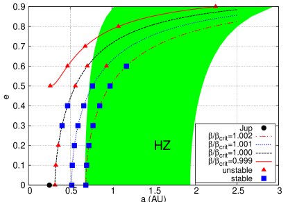
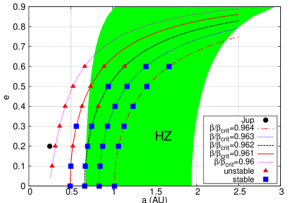
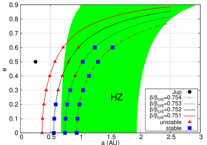
Figure 1: A comparison of Hill and Lagrange stability. Colored curves (shown also in different linestyles) are contours of ${\beta/\beta_{\mathrm{crit}}}$ (the Hill boundary lies at ${\beta/\beta_{\mathrm{crit}}}=1$). Points on the curve designate $N-$ body simulations: red points were unstable, blue stable for an Earth mass planet. The green shaded region represents the HZ, and the black point is the “known” Jupiter mass planet. The left-most curves with no stable configurations correspond to $\tau_{u}$, the right-most that are fully stable represent $\tau_{s}$. (Note that for these cases we consider eccentricities $>0.9$ in order to identify $\tau_{u}$).

In Figs. 1 & 2, we show representative results of our numerical simulations from the Jupiter mass planet with hypothetical Earth mass planet case discussed in Section 2. In all panels of Figs. 1 & 2, the blue squares and red triangles represent Lagrange stable and unstable simulations respectively, the black circle represents the “known” planet and the shaded green region represents the EHZ. For each case, we also plot ${\beta/\beta_{\mathrm{crit}}}$ contours calculated from Eq. (1). In any given panel, as $a$ increases, the curves change from all unstable (all red triangles) to all stable (all blue squares), with a transition region in between.

We designate a particular ${\beta/\beta_{\mathrm{crit}}}$ contour as $\tau_{\mathrm{s}}$, beyond which (larger values) a hypothetical terrestrial mass planet is stable for all values of $a$ and $e$, for at least $10^{7}$ years. We tested $\tau_{\mathrm{s}}$ is the first ${\beta/\beta_{\mathrm{crit}}}$ (close to the known massive planet) that is completely stable (only blue squares). For ${\beta/\beta_{\mathrm{crit}}}$ curves below $\tau_{\mathrm{s}}$, all or some locations along those curves may be unstable; hence, $\tau_{\mathrm{s}}$ is a conservative representation of the Lagrange stability boundary. Similarly, we designate $\tau_{\mathrm{u}}$ as the largest value of ${\beta/\beta_{\mathrm{crit}}}$ for which all configurations are unstable. Therefore, the range $\tau_{u}<{\beta/\beta_{\mathrm{crit}}}<\tau_{s}$ is a transition region, where the hypothetical planet’s orbit changes from unstable ($\tau_{\mathrm{u}}$) to stable ($\tau_{\mathrm{s}}$). Typically this transition occurs over $10^{-3}{\beta/\beta_{\mathrm{crit}}}$. Although Figs. 1 & 2 only show curves in this transition region, we performed many more integrations at larger and smaller values of ${\beta/\beta_{\mathrm{crit}}}$, but exclude them from the plot to improve the readability. For all cases, all our simulations with ${\beta/\beta_{\mathrm{crit}}}>\tau_{\mathrm{s}}$ are stable, and all with ${\beta/\beta_{\mathrm{crit}}}<\tau_{\mathrm{u}}$ are unstable.

These figures show that the Lagrange stability boundary significantly diverges from Hill stability boundary, as the eccentricity of the known Jupiter-mass planet increases. Moreover, $\tau_{\mathrm{s}}$ is more or less independent (within $0.1\%$) of whether the Jupiter mass planet lies at $0.25$ AU or at $4$ AU. If an extra-solar planetary system is known to have a Jupiter mass planet, then one can calculate ${\beta/\beta_{\mathrm{crit}}}$ over a range of $a$ & $e$, and those regions with ${\beta/\beta_{\mathrm{crit}}}>\tau_{\mathrm{s}}$ are stable. We show explicit examples of this methodology in Section 4.

We also consider host star masses of $0.3M_{\odot}$ and performed additional simulations. We do not show our results here, but they indicate the mass of the star does not effect stability boundaries.

3.2 Lagrange stability boundary as a function of planetary mass & eccentricity.

In this section we consider the broader range of “known” planetary masses discussed in Section 2 and listed in Table 1. Figures 1 & 2 show that as the eccentricity of the “known” planet increases, $\tau_{\mathrm{s}}$ and $\tau_{\mathrm{u}}$ appear to change monotonically. This trend is apparent on all our simulations, and suggests $\tau_{\mathrm{s}}$ and $\tau_{\mathrm{u}}$ may be described by an analytic function of the mass and eccentricity of the known planet. Therefore, instead of plotting the results from these models in $a-e$ space, as shown in Figs. 1 & 2, we identified these analytical expressions that relate $\tau_{\mathrm{s}}$ and $\tau_{\mathrm{u}}$ to mass $m_{1}$ and eccentricity $e_{1}$ of the known massive planet. Although these fits were made for planets near the host star, these fits should apply in all cases, irrespective of it’s distance from the star. In the following equations, the parameter $x=\log[m_{1}]$, where $m_{1}$ is expressed in Earth masses and $y=e_{1}$. The stability boundaries for systems with hypothetical $1{\rm\,M_{\oplus}}$ and $10{\rm\,M_{\oplus}}$ mass companion are:

$$\tau_{\mathrm{j}} = c_{1}+\frac{c_{2}}{x}+c_{3}~{}y+\frac{c_{4}}{x^{2}}+c_{5}~{}y^{2}+c_{6}~{}\frac{y}{x}+\frac{c_{7}}{x^{3}}+c_{8}~{}y^{3}+c_{9}~{}\frac{y^{2}}{x}+c_{10}~{}\frac{y}{x^{2}}$$ (2)

where $j=s,u$ indicate stable or unstable and the coefficients for each case are given Table 2.

The coefficients in the above expression were obtained by finding a best fit curve to our model data that maximizes the $R^{2}$ statistic,

$$R^{2} = 1-\frac{\displaystyle\sum_{i}^{n}(\tau^{model}_{i}-\tau^{fit}_{i})^{2}}{\displaystyle\sum_{i}^{n}(\tau^{model}_{i}-\overline{\tau^{model}})^{2}}$$ (3)

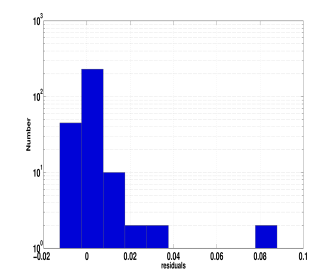
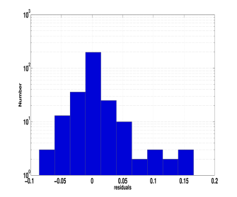
Figure 3: In the top panels, we show contours of $\tau_{\mathrm{s}}$ from numerical simulations (solid line) compared to the best fit (dashed line ) in $\log[m_{1}]$ – $e$ space, for $1{\rm\,M_{\oplus}}$ (panel a) and $10{\rm\,M_{\oplus}}$ (panel b) companions. The expression for the best fit is given in Eq. (2) with appropriate coefficients given in Table 1. The bottom panels show residuals between the numerical results and the best fit, with a standard deviation of $0.0065$ for $1{\rm\,M_{\oplus}}$ companion (panel c) and $0.0257$ for $10{\rm\,M_{\oplus}}$ companion (panel d).

where $\tau^{model}_{i}$ is the $i^{th}$model value of $\tau$ from numerical simulations, $\tau^{fit}_{i}$ is the corresponding model value from the curve fit, $\overline{\tau^{model}}$ is the average of all the $\tau_{model}$ values and $n=572$ is the number of models (including mass, eccentricity and locations of the massive planet). Values close to $1$ indicate a better quality of the fit. In Fig. 3, the top panels (a) $\&$ (b) show contour maps of $\tau_{\mathrm{s}}$ as a function of $\log[m_{1}]$ and $e_{1}$ between model data (solid line) and best fit (dashed line). The $R^{2}$ values for $1{\rm\,M_{\oplus}}$ companion (Fig. 3(a)) and $10{\rm\,M_{\oplus}}$ companion (Fig. 3(b)) are $0.99$ and $0.93$, respectively, for $\tau_{\mathrm{s}}$. In both the cases, the model and the fit deviates when the masses of both the planets are near terrestrial mass. Therefore our analysis is most robust for more unequal mass planets. The residuals between the model and the predicted $\tau_{s}$ values are also shown in Fig. 3(c) ($1{\rm\,M_{\oplus}}$ companion) $\&$ Fig. 3(d) ($10{\rm\,M_{\oplus}}$ companion). The standard deviation of these residuals is $0.0065$ and $0.0257$ for $1{\rm\,M_{\oplus}}$ and $10{\rm\,M_{\oplus}}$, respectively, though the $1{\rm\,M_{\oplus}}$ case has an outlier which does not significantly effect the fit. The maximum deviation is $0.08$ for $1{\rm\,M_{\oplus}}$ and $0.15$ for $10{\rm\,M_{\oplus}}$ cases.

The expression given in Eq. (2) can be used to identify Lagrange stable regions (${\beta/\beta_{\mathrm{crit}}}>\tau_{\mathrm{s}}$) for terrestrial mass planets around stars with one known planet with $e\leq 0.6$ and may provide an important tool for the observers to locate these planets. Once a Lagrange stability boundary is identified, it is straightforward to calculate the range of $a$ and $e$ that is stable for a hypothetical terrestrial mass planet, using Eq.(1). In the next section, we illustrate the applicability of our method for selected observed systems.

4 Application to observed systems

The expressions for $\tau_{s}$ given in §3.2 can be very useful in calculating parts of HZs that are stable for all currently known single planet systems. In order to calculate this fraction, we used orbital parameters from the Exoplanet Data Explorer maintained by California Planet Survey consortium, and selected all $236$ single planet systems in this database with masses in the range $10{\rm\,M_{jup}}$ to $10{\rm\,M_{\oplus}}$ and $e\leq 0.6$.

Table 3 lists the properties of the example systems that we consider in §4.1-§4.4, along with the orbital parameters of the known companions and stellar mass. The procedure to determine the extent of the stable region for a hypothetical $1{\rm\,M_{\oplus}}$ and $10{\rm\,M_{\oplus}}$ is as follows: (1) Identify the mass ($m_{1}$) and eccentricity ($e$) of the known planet. (2) Determine $\tau_{\mathrm{s}}$ from Eq. 2 with coefficients from Table 2. (3) Calculate ${\beta/\beta_{\mathrm{crit}}}$ over the range of orbits ($a$ and $e$) around the known planet using Eq. 1. (4) The Lagrange stability boundary is the ${\beta/\beta_{\mathrm{crit}}}=\tau_{s}$ curve.

4.1 Rho CrB

As an illustration of the internal Jupiter + Earth case, we consider the Rho CrB system. Rho CrB is a G0V star with a mass similar to the Sun, but with greater luminosity. Noyes et al. (1997) discovered a Jupiter-mass planet orbiting at a distance of $0.23$ AU with low eccentricity ($e=0.04$). Since the current inner edge of the circular HZ of this star lies at $0.90$ AU, there is a good possibility for terrestrial planets to remain stable within the HZ. Indeed, Jones et al. (2001) found that stable orbits may be prevalent in the present day circular HZ of Rho CrB for Earth mass planets.

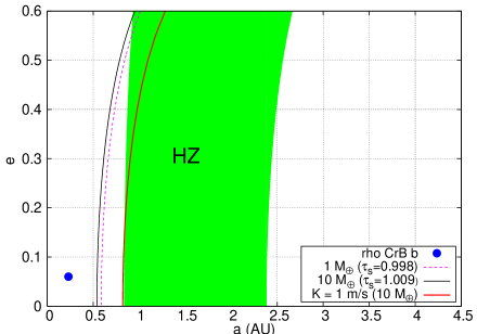
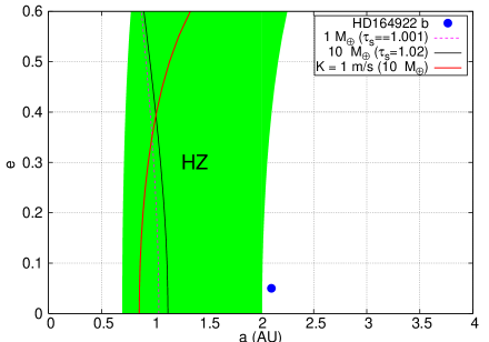
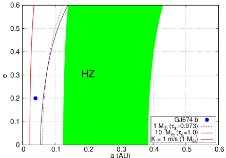
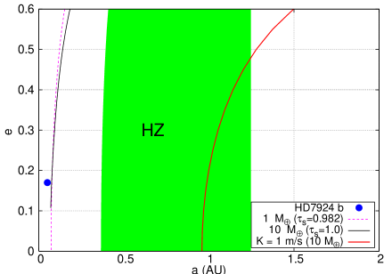
Figure 4: Comparison of Lagrange stable regions and habitable zones for four known systems. The magenta curves represent $\tau_{s}$ for a $1{\rm\,M_{\oplus}}$ planet, black $10{\rm\,M_{\oplus}}$ (c.f. Fig. 3). For panels $a$, $c$ and $d$, stable orbits lie to the right of these curves, but lie to the left in panel $b$. The red solid line shows the $1$ ms^-1 RV amplitude of a hypothetical terrestrial planet on a circular orbit. The green region is the HZ.

Fig. 4a shows the EHZ (green shaded) assuming a 50% cloud cover in the $a-e$ space of Rho CrB. The Jupiter mass planet is the blue filled circle. Corresponding $\tau_{\mathrm{s}}$ values calculated from Eq.(2) for $1{\rm\,M_{\oplus}}$ companion ($0.998$, dashed magenta line) and $10{\rm\,M_{\oplus}}$ companion ($1.009$, black solid line) are also shown. These two contours represent the stable boundary beyond which an Earth-mass or super-Earth will remain stable for all values of $a$ and $e$ (cf. Figs. 1a and 1b). The fraction of the HZ that is stable for $1{\rm\,M_{\oplus}}$ is $72.2\%$ and for $10{\rm\,M_{\oplus}}$ is $77.0\%$. Therefore the Lagrange stable stable region is larger for a larger terrestrial planet. We conclude that the HZ of rho CrB can support terrestrial-mass planets, except for very high eccentricity ($e>0.6$).

These results are in agreement with the conclusion of Jones et al. (2001) and Menou & Tabachnik (2003), who found that a planet with a mass equivalent to the Earth-moon system, when launched with $e=0$ within the HZ of Rho CrB, can remain stable for $\sim 10^{8}$ years. They also varied the mass of Rho CrB b up to $8.8{\rm\,M_{jup}}$ and still found that the HZ is stable. Our models also considered systems with $3{\rm\,M_{jup}}$, $5{\rm\,M_{jup}}$ and $10{\rm\,M_{jup}}$ and our results show that even for these high masses, if the initial eccentricity of the Earth-mass planet is less than $0.3$, then it is stable.

To show the detectability of a $10{\rm\,M_{\oplus}}$ planet, we have also drawn a radial velocity (RV) contour of 1 ms^-1 (red curve), which indicates that a $10{\rm\,M_{\oplus}}$ planet in the HZ is detectable. A similar contour for an Earth mass planet is not shown because the precision required is extremely high.

4.2 HD 164922

Butler et al. (2006) discovered a Saturn-mass planet ($0.36{\rm\,M_{jup}}$) orbiting HD 164922 with a period of 1150 days ($a=2.11$ AU) and an eccentricity of $0.1$. Although it has a low eccentricity, the uncertainty (0.14) is larger than the value itself. Therefore, the appropriate Saturn mass cases could legitimately use any $e$ in the range $0.0<e<0.25$ cases, but we use $e=0.1$.

Figure 4b, shows the stable regions in the EHZ (green shaded) of HD 164922, for hypothetical Earth (magenta) and super-Earth (black) planets. The Saturn-mass planet (blue filled circle) is also shown at 2.11 AU. About $28\%$ of the HZ in HD 164922 is stable for a $10{\rm\,M_{\oplus}}$ planet (for eccentricities $~{}\hbox to0.0pt{$<$\hss}{\lower 4.30554pt\hbox{$\sim$}}0.6$), whereas for Earth mass planets only $10\%$ of the HZ is stable. We again show the detection limit for a $10{\rm\,M_{\oplus}}$ case.

4.3 GJ 674

GJ 674 is an M-dwarf star with a mass of $0.35M_{\odot}$ and an effective temperature of $3600$ K. Bonfils et al. (2007) found a $12{\rm\,M_{\oplus}}$ with an orbital period and eccentricity of $4.69$ days ($a=0.039$ AU) and $0.20$, respectively. Fig. 4c shows the EHZ of GJ 674 in $a-e$ space. Also shown are the known planet GJ 674 b (filled blue circle), EHZ (green shaded), and detection limit for an Earth-mass planet (red curve). The values of $\tau_{\mathrm{s}}$ for $1{\rm\,M_{\oplus}}$ and $10{\rm\,M_{\oplus}}$ planets, from Eq.2, are $0.973$ (magenta) and $1.0$ (black), respectively. Notice that the fraction of the HZ that is stable for $1{\rm\,M_{\oplus}}$ is slightly greater ($79.1\%$) than $10{\rm\,M_{\oplus}}$ planet ($78.8\%$), which differs from previous systems we considered here. A similar behavior can be seen in another system (HD 7924) that is discussed in the next section. It seems that when the planet mass ratio is approaching $1$, the HZ of a $10{\rm\,M_{\oplus}}$ mass planet offers less stability at high eccentricities ($>0.6$) than a $1{\rm\,M_{\oplus}}$ planet. But as noted in §3.2, this analysis should be weighted with the fact that our fitting procedure is not as accurate for a $10{\rm\,M_{\oplus}}$ planet than a $1{\rm\,M_{\oplus}}$ planet.

4.4 HD 7924

Orbiting a K0 dwarf star at $0.057$ AU, the super-Earth HD 7924 b was discovered by NASA-UC Eta-Earth survey by the California Planet Search (CPS) group (Howard et al., 2009), in an effort to find planets in the mass range of $3-30M_{\oplus}$. It is estimated to have an $M\sin i=9.26M_{\oplus}$ with an eccentricity of $0.17$. Fig. 4d shows $\tau_{\mathrm{s}}$ values for hypothetical $10M_{\oplus}$ (magenta) and $1M_{\oplus}$ (black line) planets are $1.00$ and $0.98$, respectively. Unlike GJ 674, where only part of the HZ is stable, around $94\%$ of HD 7924’s HZ is stable for these potential planets. Furthermore, we have also plotted an RV contour of $1$ ms^-1 arising from the $10M_{\oplus}$ planet (red curve). This indicates that this planet may lie above the current detection threshold, and may even be in the HZ.

Howard et al. (2009) do find some additional best-fit period solutions with very high eccentricities ($e>0.45$), but combined with a false alarm probability (FAP) of $>20\%$, they conclude that these additional signals are probably not viable planet candidates. Further monitoring may confirm or forbid the existence of additional planets in this system.

4.5 Fraction of stable HZ

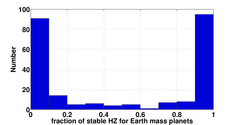
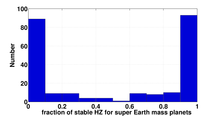
Figure 5: Distribution of fraction of stable HZ for hypothetical $1{\rm\,M_{\oplus}}$ planet (panel a) and $10{\rm\,M_{\oplus}}$ planet (panel b), in currently observed single planet systems. Of the total systems ($236$) that we considered, nearly $40\%(95)$ of the systems have $\geq 90\%$ of their HZ stable (peak near 1). About $38\%(91)$ of the systems have less than $10\%$ of their HZ stable (peak near 0). We do not consider systems that have planetary masses $>10{\rm\,M_{jup}}$ or if $e>0.6$.

For astrobiological purposes, the utility of $\tau_{\mathrm{s}}$ is multi-fold. Not only is it useful in identifying stable regions within the HZ of a given system, but it can also provide (based on the range of $a$ & $e$) what fraction of the HZ is stable. We have calculated this fraction for all single planet systems in the Exoplanet Data Explorer, as of March 25 2010. The distribution of fractions of currently known single planet systems is shown in Fig. 5 and tabulated in Table 4. A bimodal distribution can clearly be seen. Nearly $40\%$ of the systems have more than $90\%$ of their HZ stable and $38\%$ of the systems have less than $10\%$ of their HZ stable. Note that if we include systems with masses $>10{\rm\,M_{jup}}$ and also $e>0.6$ (which tend to have $a\sim 1$ AU (Wright et al., 2009)), the distribution will change and there will be relatively fewer HZs that are fully stable.

5 Summary

We have empirically determined the Lagrange stability boundary for a planetary system consisting of one terrestrial mass planet and one massive planet, with initial eccentricities less than 0.6. Our analysis shows that for two-planet systems with one terrestrial like planet and one more massive planet, Eq.(2) defines Lagrange stable configurations and can be used to identify systems with HZs stable for terrestrial mass planets. Furthermore, in Table 4 we provide a catalog of exoplanets, identifying the fraction of HZ that is Lagrange stable for terrestrial mass planets. A full version of the table is available in the electronic edition of the journal.

In order to identify stable configurations for a terrestrial planet, one can calculate a stability boundary (denoted as $\tau_{\mathrm{s}}$ from Eq.(2)) for a given system (depending on the eccentricity and mass of the known planet), and calculate the range of $a$ & $e$ that can support a terrestrial planet, as shown in Section 4. For the transitional region between unstable to stable ($\tau_{\mathrm{u}}<{\beta/\beta_{\mathrm{crit}}}<\tau_{\mathrm{s}}$), a numerical integration should be made. Our results are in general agreement with previous studies (Menou & Tabachnik, 2003), (Jones et al., 2006) & (Sándor et al., 2007), but crucially our approach does not (usually) require a large suite of N-body integrations to determine stability.

We have only considered two-planet systems, but the possibility that the star hosts more, currently undetected planets is real and may change the stability boundaries outlined here. However, the presence of additional companions will likely decrease the size of the stable regions shown in this study. Therefore, those systems that have fully unstable HZs from our analysis will likely continue to have unstable HZs as more companions are detected (assuming the mass and orbital parameters of the known planet do not change with these additional discoveries). The discovery of an additional planet outside the HZ that destabilizes the HZ is also an important information.

As more extra-solar planets are discovered, the resources required to follow-up grows. Furthermore, as surveys push to lower planet masses, time on large telescopes is required, which is in limited supply. The study of exoplanets seems poised to transition to an era in which systems with the potential to host terrestrial mass planets in HZs will be the focus of surveys. With limited resources, it will be important to identify systems that can actually support a planet in the HZ. The parameter $\tau_{s}$ can therefore guide observers as they hunt for the grand prize in exoplanet research, an inhabited planet.

Although the current work focuses on terrestrial mass planets, the same analysis can be applied to arbitrary configurations that cover all possible orbital parameters. Such a study could represent a significant improvement over the work of Barnes & Greenberg (2007). The results presented here show that ${\beta/\beta_{\mathrm{crit}}}=1$ is not always the Lagrange stability boundary, as they suggested. An expansion of this research to a wider range of planetary and stellar masses and larger eccentricities could provide an important tool for determining the stability and packing of exoplanetary systems. Moreover, it could reveal an empirical relationship that describes the Lagrange stability boundary for two planet systems. As new planets are discovered in the future, the stability maps presented here will guide future research on the stability of extra-solar planetary systems.

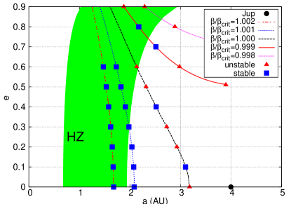
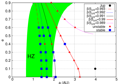
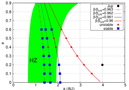
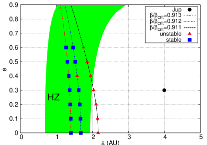
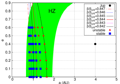
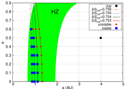
Figure 2: Same as Fig. 1, only now the Jupiter mass planet is at 4 AU. The range of values of $\tau_{\mathrm{s}}$ is approximately the same as in Fig. 1: from $1.002-0.756$.

Table 1: Properties of systems considered in this study.

“Known” Planet	a (AU)
10 Mjup	(0.25, 4)
5.6 Mjup	(0.25, 4)
3 Mjup	(0.25, 4)
1.77 Mjup	(0.25, 4)
1 Mjup	(0.25, 4)
1.86 MSat	(0.5, 2)
1 MSat	(0.5, 2)
56 ${\rm\,M_{\oplus}}$	(0.5, 2)
30 ${\rm\,M_{\oplus}}$	(0.5, 2)
17.7 ${\rm\,M_{\oplus}}$	(0.5, 2)
10 ${\rm\,M_{\oplus}}$	(0.5, 2)

Table 2: Best fit properties for Eq.2.

$1{\rm\,M_{\oplus}}$                  $10{\rm\,M_{\oplus}}$
Coefficients	$\tau_{\mathrm{s}}$	$\tau_{\mathrm{u}}$	$\tau_{\mathrm{s}}$	$\tau_{\mathrm{u}}$
$c_{1}$	1.0018	1.0098	0.9868	1.0609
$c_{2}$	-0.0375	-0.0589	0.0024	-0.3547
$c_{3}$	0.0633	0.04196	0.1438	0.0105
$c_{4}$	0.1283	0.1078	0.2155	0.6483
$c_{5}$	-1.0492	-1.0139	-1.7093	-1.2313
$c_{6}$	-0.2539	-0.1913	-0.2485	-0.0827
$c_{7}$	-0.0899	-0.0690	-0.1827	-0.4456
$c_{8}$	-0.0316	-0.0558	0.1196	-0.0279
$c_{9}$	0.2349	0.1932	1.8752	0.9615
$c_{10}$	0.2067	0.1577	-0.0289	0.1042
$R^{2}$	0.996	0.997	0.931	0.977
$\sigma$	0.0065	0.0061	0.0257	0.0141
Max. dev.	0.08	0.08	0.15	0.05

Table 3: Observed parameters of example systems presented in §4.

System	M $\sin i$	a (AU)	e	$M_{\star}(M_{\odot})$
Rho CrB	1.06 $M_{\mathrm{jup}}$	0.23	0.06 ($\pm$ 0.028)	0.97
HD 164922	0.36 $M_{\mathrm{jup}}$	2.11	0.05 ($\pm$ 0.14)	0.94
GJ 674	12 ${\rm\,M_{\oplus}}$	0.039	0.20 ($\pm$ 0.02)	0.35
HD 7924	9.26 ${\rm\,M_{\oplus}}$	0.057	0.17 ($\pm$ 0.16)	0.832

Table 4: Lagrange stable ($\tau_{\mathrm{s}}$) and unstable ($\tau_{\mathrm{u}}$) boundaries, and the corresponding fraction of habitable zone (FHZ) stable for terrestrial mass planets in known single planet systems. A full version of the table is available in the electronic edition of the Astrophysical Journal.

System	$m_{\mathrm{1}}(M_{\mathrm{jup}})$	a (AU)	e	$\tau_{\mathrm{s}}$	$\tau_{\mathrm{u}}$	FHZ	$\tau_{\mathrm{s}}$	$\tau_{\mathrm{u}}$	FHZ
				$(1{\rm\,M_{\oplus}})$	$(1{\rm\,M_{\oplus}})$	$(1{\rm\,M_{\oplus}})$	$(10{\rm\,M_{\oplus}})$	$(10{\rm\,M_{\oplus}})$	$(10{\rm\,M_{\oplus}})$
HD 142b	1.3057	1.04292	0.26	0.9347	0.9323	0.000	0.9552	0.9320	0.000
HD 1237	3.3748	0.49467	0.51	0.7407	0.7401	0.213	0.7549	0.7450	0.000
HD 1461	0.0240	0.06352	0.14	0.9920	0.9780	0.976	1.0200	0.9200	0.959
WASP-1	0.9101	0.03957	0.00	1.0022	0.9990	0.990	1.0200	0.9980	0.991
HIP 2247	5.1232	1.33884	0.54	0.7138	0.7111	0.000	0.7490	0.7387	0.000

References

- Barnes & Quinn (2004) Barnes, R., & Quinn, T. 2004, ApJ, 611, 494
- Barnes & Raymond (2004) Barnes, R., & Raymond, S. 2004, ApJ, 617, 569
- Barnes & Greenberg (2006) Barnes, R., & Greenberg, R. 2006, ApJ, 665, L163
- Barnes & Greenberg (2007) Barnes, R., & Greenberg, R. 2007, ApJ, 665, L67
- Barnes et al. (2008b) Barnes et al. 2008b, AsBio, 8, 557
- Barnes et al. (2009) Barnes, R., Jackson., B., Greenberg, R., & Raymond, S. 2009, ApJ, 700, L30
- Bonfils et al. (2007) Bonfils, X. et al. 2007, A&A, 474, 293
- Bouchy et al. (2008) Bouchy, F et al. 2008, arXiv0812.1608
- Butler et al. (2004) Butler, P. et al. 2004, ApJ, 617, 580
- Butler et al. (2006) Butler, R. P. et al. 2006, ApJ, 646, 505
- Chambers (1996) Chambers, J. E. 1996, Icarus, 119, 261
- Chambers (1999) Chambers, J. E. 1999, MNRAS, 304, 793
- Cuntz & Yeager (2009) Cuntz, M., & Yeager, K. E. 2009, ApJ, 697, 86
- Ford et al. (2005) Ford, E. B., Lystad, V. & Rasio, F. A. 2005, Nature, 434, 873
- Gladman (1993) Gladman, B. 1993, Icarus, 106, 247
- Goździewski et al. (2001) Goździewski2002, K., Bois, E., Maciejewski, A. J., & Kiseleva-Eggleton, L. 2001, A&A, 78, 569
- Hart (1978) Hart, M. H. 1978, Icarus, 33, 23
- Howard et al. (2009) Howard, A. W. et al. 2009, ApJ, 696,75
- Huang (1959) Huang, S. S. 1959, American Scientist, 47, 397
- Ji et al. (2002) Ji, J. et al. 2002, ApJ, 572, 1041
- Jones et al. (2001) Jones, B. W., Sleep, P. N., & Chambers, J. E. 2001, A&A, 366, 254
- Jones et al. (2006) Jones, B. W., Sleep, P. N., & Underwood, D. R. 2006, ApJ, 649, 1010
- Kasting et al. (1993) Kasting, J. F., et al. 1993, Icarus, 101, 108
- Kopparapu et al. (2009) Kopparapu, R., Raymond, S. N., & Barnes, R. 2009, ApJ, 695, L181
- Laskar (1989) Laskar, J. 1989, Nature, 338, 237
- Laughlin & Chambers (2001) Laughlin, G., & Chambers, J. E. 2001, ApJ, 551, L109
- Marchal & Bozis (1982) Marchal, C. & Bozis, G. 1982, CeMech, 26, 311
- Marcy et al. (2005a) Marcy, G et al. 2005a, Prog, Theor. Phys. Suppl., 158, 24
- Mayor et al. (2009) Mayor, M. et al. 2009, A&A
- Menou & Tabachnik (2003) Menou, K., & Tabachnik, S. 2003, ApJ, 583, 473
- Noyes et al. (1997) Noyes, R, W. et al. (1997), ApJ, 483, 111
- Ramsey et al. (1998) Ramsey, L. W., et al. 1998, Proc. SPIE, 3352, 34
- Rasio & Ford (1996) Rasio, F. A. & Ford, E. B. 1996, Science, 274, 954
- Raymond et al. (2006) Raymond, S. N., & Barnes, R. 2005, ApJ, 619, 549
- Raymond et al. (2009) Raymond, S. N., Barnes, R., Veras, D., Armitage, P. J., Gorelick, N., & Greenberg, R. 2009, ApJ, 696, L98
- Ruden (1999) Ruden, S. P. 1999, in The Origin of Stars and Planetary Systems, ed. Lada, C. J. & Kylafis, N. D. (Dordrecht: Kluwer), 643
- Sándor et al. (2007) Sándor, Zs., Suli, Á., Érdi, B., Pilat-Lohinger, E., & Dvorak, R. 2007, MNRAS, 375, 1495
- Selsis et al. (2007) Selsis, F. et al. (2007), A & A, 476, 137
- Udry et al. (2007) Udry, S. et al. 2007, A & A, 469, L43
- von Bloh et al. (2007) von Bloh, W. et al. 2007, A&A, 476, 1365
- Williams et al. (1997) Williams, D. M., Kasting, J. F., & Wade, R. A. 1997, Nature, 385, 234
- William & Pollard (2002) Williams, D. M., & Pollard, D. 2002, International Journal of Astrobiology, 1, 61
- Wisdom (1982) Wisdom, J. 1982, AJ, 87, 577
- Wittenmyer et al. (2009) Wittenmyer, R. A. 2009, arXiv0903.0652
- Wright et al. (2007) Wright, J, T., et al. 2007, ApJ, 657, 533
- Wright et al. (2009) Wright, J, T., et al. 2010, ApJ, 693, 1084