Localization of the SFT inspired Nonlocal Linear Models and Exact Solutions

Abstract

A general class of gravitational models driven by a nonlocal scalar field with a linear or quadratic potential is considered. We study the action with an arbitrary analytic function $\mathcal{F}(\Box_{g})$, which has both simple and double roots. The way of localization of nonlocal Einstein equations is generalized on models with linear potentials. Exact solutions in the Friedmann–Robertson–Walker and Bianchi I metrics are presented.

1 Introduction

Recently a wide class of nonlocal cosmological models based on the string field theory (SFT) (for details see reviews [1]) and the $p$-adic string theory [2] emerges and attracts a lot of attention [3]–[21]. Due to the presence of phantom excitations nonlocal models are of interest for the present cosmology. Generally speaking, models that violate the null energy condition (NEC) have ghosts, and therefore are unstable and physically unacceptable. Phantom fields look harmful to the theory and a local model with a phantom scalar field is not acceptable from the general point of view. Models with higher derivative terms produce well-known problems with quantum instability [22, 23]. A idea that could solve the problems is that terms with high order derivatives can be treated as corrections valued only at small energies below the physical cut-off [24, 25]. This approach implies the possibility to construct a UV completion of the theory and requires detailed analysis.

Note that the possibility of the existence of dark energy with $w_{\mathrm{DE}}<-1$ is not excluded experimentally. Contemporary cosmological observational data [26] strongly support that the present Universe exhibits an accelerated expansion providing thereby an evidence for a dominating dark energy component with the state parameter

$$w_{\mathrm{DE}}={}-1.0\pm 0.2.$$ (1)

The present cosmological observations do not exclude an evolving parameter $w_{\mathrm{DE}}$. Moreover, the recent analysis of the observation data indicates that the varying in time dark energy with the state parameter $w_{\mathrm{DE}}$, which crosses the cosmological constant barrier, gives a better fit than a cosmological constant [27] (see also [28, 29] and references therein).

To obtain a stable model with $w_{\mathrm{DE}}<-1$ one should construct the effective theory with the NEC violation from the fundamental theory, which is stable and admits quantization. From this point of view the NEC violation might be a property of a model that approximates the fundamental theory and describes some particular features of the fundamental theory. With the lack of quantum gravity, we can just trust string theory or deal with an effective theory admitting the UV completion. It can be considered as a hint towards the SFT inspired cosmological models (details about the string cosmology see in reviews [30]). Note also, that not only the string inspired cosmological models obey nonlocality [31].

In the flat space-time nonlocal equations are actively investigated as well [32, 33, 34, 35]. Note that differential equations of infinite order were began to study long time ago [36, 37].

The purpose of this paper is to study gravitational models with a nonlocal scalar field. We consider a general form of a nonlocal action for the scalar field with a quadratic or linear potential, keeping the main ingredient, the analytic function $\mathcal{F}(\Box_{g})$, which in fact produces the nonlocality in question, almost unrestricted.

The possible way to find solutions of the Einstein equations with a quadratic potential of the nonlocal scalar field, is to reduce them to a system of Einstein equations describing many non-interacting local scalar fields [7, 14] (see also [18, 20]). Some of the obtained local scalar fields are normal and other of them are phantom ones. In this paper we generalize the algorithm of localization, proposed in [14, 20], on the case of a linear potential. Note that the way of localization in the case of a linear potential and in the case of a quadratic potential with a linear term, considered in [16], are different.

The paper is organized as follows. In Section 2 we describe nonlocal cosmological models. In Section 3 we propose the algorithm to find particular solutions of the nonlocal Einstein equations, solving only local ones, and prove the self-consistence of it. Any solution for the obtained system of differential equations is a particular solution for the initial nonlocal Einstein equations. Exact solutions in the Friedmann–Robertson–Walker and Bianchi I metrics are presented in Section 4. In Section 5 we summarize the obtained results and propose directions for further investigations.

2 Model setup

The four-dimensional action with a quadratic or linear potential, motivated by the string field theory, has been studied in [7, 8, 14, 15, 16, 18, 20, 21]. Such a model appears as a linearization of the SFT inspired model in the neighborhood of an extremum of the potential (see [18] for details). For linear models, solving the nonlocal equations using the technique, proposed in [14], is completely equivalent to solving the equations using the diffusion-like partial differential equations [16]. By linearizing a nonlinear model about a particular field value, one is able to specify initial data for nonlinear models, which he then evolves into the full nonlinear regime using the diffusion-like equation [16].

In this paper we study nonlocal cosmological models with a quadratic potential, in other words, a linear nonlocal model, which can be described by the following action:

$$S=\int d^{4}x\sqrt{-g}\left(\frac{R}{16\pi G_{N}}+\frac{1}{g_{o}^{2}}\left(\frac{1}{2}\phi\mathcal{F}(\Box_{g})\phi-V(\phi)\right)-\Lambda\right),$$ (2)

where $G_{N}$ is the dimensionless gravitational constant: $G_{N}=1/(8\pi M_{P}^{2}\alpha^{\prime})$, $M_{P}$ is the Planck mass and $\alpha^{\prime}$ is the string length squared. The dimensionless parameter $g_{o}$ is the open string coupling constant divided on $\sqrt{\alpha^{\prime}}$. We use dimensionless coordinates $x_{\mu}$ and the signature $(-,+,+,+)$. $R$ is the scalar curvature, $g_{\mu\nu}$ is the metric tensor, $\Lambda$ is a dimensionless constant. The potential is an arbitrary quadratic polynomial: $V(\phi)=C_{2}\phi^{2}+C_{1}\phi+C_{0}$. The Beltrami–Laplace (d’Alembert) operator $\Box_{g}$ is applied to scalar functions and can be written as follows

$$\Box_{g}=\frac{1}{\sqrt{-g}}\partial_{\mu}\sqrt{-g}g^{\mu\nu}\partial_{\nu}\,.$$ (3)

The function $\mathcal{F}$ is assumed to be an analytic function, therefore, one can represent it by the convergent series expansion:

$$\mathcal{F}(\Box_{g})=\sum\limits_{n=0}^{\infty}f_{n}\Box_{g}^{\;n},$$ (4)

where $f_{n}$ are constants. The function $\mathcal{F}$ may have infinitely many roots manifestly producing thereby the nonlocality [13, 18]. This model has been studied in [7, 18] with an additional condition that all roots of the function $\mathcal{F}$ are simple. In this paper we consider double roots as well. To clarify the interest to consider the case of double roots let us study a trivial example with

$$\mathcal{F}(\Box_{g})=(\Box_{g}-J_{1})(\Box_{g}-J_{2}),$$ (5)

where $J_{1}$ and $J_{2}$ are nonzero constants.

In the Minkowski space–time for $\phi$, depending only on time, we obtain the following equation of motion

$$(\partial_{t}^{2}-J_{1})(\partial_{t}^{2}-J_{2})\phi(t)=0.$$ (6)

This fourth order differential equation is equivalent to the following system of two second order equations:

$$(\partial_{t}^{2}-J_{1})\xi(t)=0,\qquad(\partial_{t}^{2}-J_{2})\phi(t)=\xi(t).$$ (7)

The first equation has the general solution

$$\xi(t)=B_{1}e^{\sqrt{J_{1}}t}+B_{2}e^{-\sqrt{J_{1}}t},$$ (8)

where $B_{1}$ and $B_{2}$ are arbitrary constants. So, we get the following second order equation in $\phi$

$$(\partial_{t}^{2}-J_{2})\phi(t)=B_{1}e^{\sqrt{J_{1}}t}+B_{2}e^{-\sqrt{J_{1}}t}.$$ (9)

In the non-resonance case (two simple roots $J_{1}$ and $J_{2}$) we get

$$\phi(t)=\frac{B_{1}}{J_{1}-J_{2}}e^{\sqrt{J_{1}}t}+\frac{B_{2}}{J_{1}-J_{2}}e^{-\sqrt{J_{1}}t}+B_{3}e^{\sqrt{J_{2}}t}+B_{4}e^{-\sqrt{J_{2}}t},$$ (10)

whereas in the resonance case (one double root $J_{2}=J_{1}$) the general solution is

$$\phi(t)=\frac{B_{1}}{2\sqrt{J_{1}}}te^{\sqrt{J_{1}}t}-\frac{B_{2}}{2\sqrt{J_{1}}}te^{-\sqrt{J_{1}}t}+B_{3}e^{\sqrt{J_{1}}t}+B_{4}e^{-\sqrt{J_{1}}t},$$ (11)

where $B_{3}$ and $B_{4}$ are arbitrary constants. This trivial example shows that behavior of solutions in the cases of one double root and two simple roots are essentially different and one can not approximate double roots by two simple roots, which are at a very small distance. Resonance phenomenons are important and actively studied in various domains of physics.

3 Algorithm of localization

3.1 Einstein equations

From action (2) we obtain the following equations

$$R_{\mu\nu}-\frac{1}{2}Rg_{\mu\nu} = 8\pi G_{N}\left(T_{\mu\nu}-\Lambda g_{\mu\nu}\right),$$ (12)

$$\mathcal{F}(\Box_{g})\phi = \frac{dV}{d\phi},$$ (13)

where $R_{\mu\nu}$ is the Ricci tensor.

The energy–momentum (stress) tensor $T_{\mu\nu}$, which is calculated by the standard formula

$$T_{\mu\nu}={}-\frac{2}{\sqrt{-g}}\frac{\delta{S}}{\delta g^{\mu\nu}},$$ (14)

can be presented in the following form:

$$T_{\mu\nu}=\frac{1}{g_{o}^{2}}\Bigl{(}E_{\mu\nu}+E_{\nu\mu}-g_{\mu\nu}\left(g^{\rho\sigma}E_{\rho\sigma}+W\right)\Bigr{)},$$ (15)

where

$$E_{\mu\nu}\equiv\frac{1}{2}\sum_{n=1}^{\infty}f_{n}\sum_{l=0}^{n-1}\partial_{\mu}\Box_{g}^{l}\phi\partial_{\nu}\Box_{g}^{n-1-l}\phi,$$ (16)

$$W\equiv\frac{1}{2}\sum_{n=2}^{\infty}f_{n}\sum_{l=1}^{n-1}\Box_{g}^{l}\phi\Box_{g}^{n-l}\phi-\frac{f_{0}}{2}\phi^{2}+V(\phi).$$ (17)

In the case of the zero potential $V(\phi)=0$, using the equation

$$F(\Box_{g})\phi=0,\quad\Longleftrightarrow\quad f_{0}\phi={}-\sum\limits_{n=1}^{\infty}f_{n}\Box_{g}^{\;n}\phi,$$ (18)

one can obtain that $W$ for $V(\phi)=0$ is equal to

$$W_{0}=\frac{1}{2}\sum_{n=1}^{\infty}f_{n}\sum_{l=0}^{n-1}\Box_{g}^{l}\phi\Box_{g}^{n-l}\phi.$$ (19)

The formula for energy–momentum tensor with $W_{0}$ has been proposed in [7] (see also [18]).

The main idea of finding the solutions to the equations of motion is to start with equation (13) for $V(\phi)=0$ and to solve it, assuming the function $\phi$ is an eigenfunction of the Beltrami–Laplace operator $\Box_{g}$. If $\Box_{g}\phi=J\phi$, then such a function $\phi$ is a solution to (13) if and only if

$$\mathcal{F}(J)=0.$$ (20)

The latter condition is known as the characteristic equation. Note that values of roots of $\mathcal{F}(J)$ do not depend on the metric. In this paper we show how the case of an arbitrary quadratic potential $V(\phi)$ can be analyzed with the help of roots of the function $\mathcal{F}(J)$.

Let us denote simple roots of $\mathcal{F}$ as $J_{i}$ and double roots of $\mathcal{F}$ as $\tilde{J}_{k}$. A particular solution of equation (13) we seek in the following form

$$\phi_{0}=\sum\limits_{i=1}^{N_{1}}\phi_{i}+\sum\limits_{k=1}^{N_{2}}\tilde{\phi}_{k},$$ (21)

where

$$(\Box_{g}-J_{i})\phi_{i}=0,\qquad(\Box_{g}-\tilde{J}_{k})^{2}\tilde{\phi}_{k}=0.$$ (22)

The fourth order differential equation $(\Box_{g}-\tilde{J_{k}})(\Box_{g}-\tilde{J_{k}})\tilde{\phi}_{k}=0$ is equivalent to the following system of the second order equations:

$$(\Box_{g}-\tilde{J_{k}})\tilde{\phi}_{k}=\varphi_{k},\qquad(\Box_{g}-\tilde{J_{k}})\varphi_{k}=0.$$ (23)

Without loss of generality we assume that for any $i_{1}$ and $i_{2}\neq i_{1}$ conditions $J_{i_{1}}\neq J_{i_{2}}$ and ${\tilde{J}}_{i_{1}}\neq{\tilde{J}}_{i_{2}}$ are satisfied.

3.2 Zero potential $V(\phi)$

It is convenient to consider the cases $C_{1}=0$ and $C_{1}\neq 0$ separately. In this subsection we consider the case of zero potential ($C_{1}=0$), the case of a linear potential is considered in the next subsection.

Modifying values of $f_{0}$ and $\Lambda$, we can transform action (2) with the potential $V(\phi)=C_{2}\phi^{2}+C_{0}$ to the action with zero potential. So, without loss of generality, we can put $C_{2}=0$ and $C_{0}=0$ and use the energy–momentum tensor for $\phi_{0}$, which has been calculated in [20]. It has been obtained that for any analytical function $\mathcal{F}(J)$, which has simple roots $J_{i}$ and double roots $\tilde{J}_{k}$, and any $\phi_{0}$ given by (21) the energy–momentum tensor

$$T_{\mu\nu}\left(\phi_{0}\right)=T_{\mu\nu}\left(\sum\limits_{i=1}^{N_{1}}\phi_{i}+\sum\limits_{k=1}^{N_{2}}\tilde{\phi}_{k}\right)=\sum\limits_{i=1}^{N_{1}}T_{\mu\nu}(\phi_{i})+\sum\limits_{k=1}^{N_{2}}T_{\mu\nu}(\tilde{\phi}_{k}),$$ (24)

where all $T_{\mu\nu}$ are given by (15) and

$$E_{\mu\nu}(\phi_{i})=\frac{{\mathcal{F}^{\prime}(J_{i})}}{2}\partial_{\mu}\phi_{i}\partial_{\nu}\phi_{i},\qquad W(\phi_{i})=\frac{J_{i}\mathcal{F}^{\prime}(J_{i})}{2}\phi_{i}^{2},$$ (25)

$$E_{\mu\nu}(\tilde{\phi}_{k})=\frac{{\mathcal{F}^{\prime\prime}(\tilde{J}_{k})}}{4}\left(\partial_{\mu}\tilde{\phi}_{k}\partial_{\nu}\varphi_{k}+\partial_{\nu}\tilde{\phi}_{k}\partial_{\mu}\varphi_{k}\right)+\frac{\mathcal{F}^{\prime\prime\prime}(\tilde{J}_{k})}{12}\partial_{\mu}\varphi_{k}\partial_{\nu}\varphi_{k},$$ (26)

$$W(\tilde{\phi_{k}})=\frac{\tilde{J}_{k}\mathcal{F}^{\prime\prime}(\tilde{J}_{k})}{2}\tilde{\phi}_{k}\varphi_{k}+\left(\frac{{\tilde{J}_{k}\mathcal{F}^{\prime\prime\prime}(\tilde{J}_{k})}}{12}+\frac{{\mathcal{F}^{\prime\prime}(\tilde{J}_{k})}}{4}\right)\varphi_{k}^{2},$$ (27)

where a prime denotes a derivative with respect to $J$: $\mathcal{F}^{\prime}\equiv\frac{d\mathcal{F}}{dJ}$,  $\mathcal{F}^{\prime\prime}\equiv\frac{d^{2}\mathcal{F}}{dJ^{2}}$ and $\mathcal{F}^{\prime\prime\prime}\equiv\frac{d^{3}\mathcal{F}}{dJ^{3}}$. The result has been obtained for an arbitrary metric.

Considering the following local action

$$S_{loc}=\int d^{4}x\sqrt{-g}\left(\frac{R}{16\pi G_{N}}-\Lambda\right)+\sum_{i=1}^{N_{1}}S_{i}+\sum_{k=1}^{N_{2}}\tilde{S}_{k},$$ (28)

where

$$S_{i}=\!{}-\frac{1}{g_{o}^{2}}\int d^{4}x\sqrt{-g}\frac{\mathcal{F}^{\prime}(J_{i})}{2}\left(g^{\mu\nu}\partial_{\mu}\phi_{i}\partial_{\nu}\phi_{i}+J_{i}\phi_{i}^{2}\right),$$ (29)

$$\begin{array}[]{rl}\!\displaystyle\tilde{S}_{k}=&\!\displaystyle\!{}-\frac{1}{g_{o}^{2}}\int d^{4}x\sqrt{-g}\left(g^{\mu\nu}\left(\frac{{\mathcal{F}^{\prime\prime}(\tilde{J}_{k})}}{4}\left(\partial_{\mu}\tilde{\phi}_{k}\partial_{\nu}\varphi_{k}+\partial_{\nu}\tilde{\phi}_{k}\partial_{\mu}\varphi_{k}\right)+{}\right.\right.\\ \displaystyle+&\displaystyle\left.\frac{\mathcal{F}^{\prime\prime\prime}(\tilde{J}_{k})}{12}\partial_{\mu}\varphi_{k}\partial_{\nu}\varphi_{k}\right)+\left.\frac{\tilde{J}_{k}\mathcal{F}^{\prime\prime}(\tilde{J}_{k})}{2}\tilde{\phi}_{k}\varphi_{k}+\left(\frac{{\tilde{J}_{k}\mathcal{F}^{\prime\prime\prime}(\tilde{J}_{k})}}{12}+\frac{{\mathcal{F}^{\prime\prime}(\tilde{J}_{k})}}{4}\right)\varphi_{k}^{2}\right),\end{array}$$ (30)

we can see that solutions of the Einstein equations and equations in $\phi_{k}$, $\tilde{\phi}_{k}$ and $\varphi_{k}$, obtained from this action, solves the initial system of nonlocal equations (12) and (13). Thus, one can find special solutions of nonlocal equations solving a system of local (differential) equations.

To clarify physical interpretation of local fields $\tilde{\phi}_{k}$ and $\varphi_{k}$, we diagonalize the kinetic terms of these scalar fields in (28). Expressing $\tilde{\phi}_{k}$ and $\varphi_{k}$ in terms of new fields $\xi_{k}$ and $\chi_{k}$:

$$\begin{split}\tilde{\phi}_{k}&=\frac{1}{2\mathcal{F}^{\prime\prime}(\tilde{J}_{k})}\left(\left(\mathcal{F}^{\prime\prime}(\tilde{J}_{k})-\frac{1}{3}\mathcal{F}^{\prime\prime\prime}(\tilde{J}_{k})\right)\xi_{k}-\left(\mathcal{F}^{\prime\prime}(\tilde{J}_{k})+\frac{1}{3}\mathcal{F}^{\prime\prime\prime}(\tilde{J}_{k})\right)\chi_{k}\right),\\ \varphi_{k}&=\xi_{k}+\chi_{k},\end{split}$$ (31)

we obtain the corresponding $\tilde{S}_{k}$ in the following form:

$$\begin{array}[]{l}\displaystyle\tilde{S}_{k}={}-\frac{1}{g_{o}^{2}}\int d^{4}x\sqrt{-g}\left(g^{\mu\nu}\frac{\mathcal{F}^{\prime\prime}(\tilde{J}_{k})}{4}\left(\partial_{\mu}\xi_{k}\partial_{\nu}\xi_{k}-\partial_{\nu}\chi_{k}\partial_{\mu}\chi_{k}\right)+{}\right.\\ \displaystyle{}+\frac{\tilde{J}_{k}}{4}\left(\left(\mathcal{F}^{\prime\prime}(\tilde{J}_{k})-\frac{1}{3}\mathcal{F}^{\prime\prime\prime}(\tilde{J}_{k})\right)\xi_{k}-\left(\mathcal{F}^{\prime\prime}(\tilde{J}_{k})+\frac{1}{3}\mathcal{F}^{\prime\prime\prime}(\tilde{J}_{k})\right)\chi_{k}\right)(\xi_{k}+\chi_{k})+{}\\ \displaystyle{}+\left.\left(\frac{{\tilde{J}_{k}\mathcal{F}^{\prime\prime\prime}(\tilde{J}_{k})}}{12}+\frac{{\mathcal{F}^{\prime\prime}(\tilde{J}_{k})}}{4}\right)(\xi_{k}+\chi_{k})^{2}\right).\end{array}$$ (32)

It is easy to see that each $\tilde{S}_{k}$ includes one phantom scalar field and one standard scalar field. So, in the case of one double root we obtain a quintom model. In the Minkowski space appearance of phantom fields in models, when $\mathcal{F}(\Box)$ has a double root, has been obtained in [32]. If $\mathcal{F}(J)$ has simple real roots, then positive and negative values of $\mathcal{F}^{\prime}(J_{i})$ alternate, so we can obtain phantom fields and, in the case of two simple roots, a quintom model.

Remark 1. If $\mathcal{F}(J)$ has an infinity number of roots then one nonlocal model corresponds to infinity number of different local models. In this case the initial nonlocal action (2) generates infinity number of local actions (28).

Remark 2. We should prove that the way of localization is self-consistent. To construct local action (28) we assume that equations (22) are satisfied. Therefore, the method of localization is correct only if these equations can be obtained from the local action $S_{loc}$. The straightforward calculations show that

$$\frac{\delta{S_{loc}}}{\delta\phi_{i}}=0\quad\Leftrightarrow\quad\Box_{g}\phi_{i}=J_{i}\phi_{i};\qquad\frac{\delta{S_{loc}}}{\delta\tilde{\phi}_{k}}=0\quad\Leftrightarrow\quad\Box_{g}\varphi_{k}=\tilde{J}_{k}\varphi_{k}.$$ (33)

Using (33) we obtain

$$\frac{\delta{S_{loc}}}{\delta\varphi_{k}}=0\qquad\Leftrightarrow\qquad\Box_{g}\tilde{\phi}_{k}=\tilde{J}_{k}\tilde{\phi}_{k}+\varphi_{k}.$$ (34)

So, the way of localization is self-consistent in the case of $\mathcal{F}(J)$ with simple and double roots [20]. The self-consistence of similar approach for $\mathcal{F}(J)$ with only simple roots has been proven in [14, 18].

In spite of the above-mention equations we obtain from $S_{loc}$ the Einstein equations:

$$G_{\mu\nu}=8\pi G_{N}\left(T_{\mu\nu}(\phi_{0})-\Lambda g_{\mu\nu}\right),$$ (35)

where $\phi_{0}$ is given by (21) and $T_{\mu\nu}(\phi_{0})$ can be calculated by (24).

So, we have obtained such systems of differential equations that any solutions of these systems are particular solutions of the initial nonlocal equations (12) and (13).

3.3 Linear potential $V(\phi)$

Let us consider the model with action (2) in the case $C_{1}\neq 0$. For the string field theory inspired form of $\mathcal{F}(\Box)$ the case $f_{0}\neq 0$ has been considered in [16]. In this case the effective potential: $-f_{0}\phi^{2}/2+V(\phi)+\Lambda$, is a quadratic potential. Using the condition $f_{0}\neq 0$, we boil down the case with an arbitrary $C_{1}$ to the case with $C_{1}=0$. Indeed, we work in a new scalar field

$$\chi=\phi-\frac{C_{1}}{f_{0}}$$ (36)

and get the energy–momentum tensor in the form (15) with

$$E_{\mu\nu}=\frac{1}{2}\sum_{n=1}^{\infty}f_{n}\sum_{l=0}^{n-1}\partial_{\mu}\Box_{g}^{l}\chi\partial_{\nu}\Box_{g}^{n-1-l}\chi,$$ (37)

$$W=\frac{1}{2}\sum_{n=1}^{\infty}f_{n}\sum_{l=1}^{n-1}\Box_{g}^{l}\chi\Box_{g}^{n-l}\chi-\frac{f_{0}}{2}\chi^{2}+\frac{C_{1}^{2}}{2f_{0}}.$$ (38)

It is easy to see that

$$\mathcal{F}(\Box)\phi=C_{1}\qquad\Longleftrightarrow\qquad\mathcal{F}(\Box)\chi=0.$$ (39)

The constant $C_{1}^{2}/(2f_{0})$ can be consider as a part of the cosmological constant. Thus, in terms of $\chi$ we obtain a model without linear term and can conclude that at $f_{0}\neq 0$ the adding of a linear term to the potential shifts the scalar field on the constant and changes the value of the cosmological constant.

Let us consider the case $f_{0}=0$. In this case $J=0$ is a root of the characteristic equation (20). It is easy to show, that the function

$$\tilde{\chi}=\phi_{0}+\psi,$$ (40)

where $\phi_{0}$ and $\psi$ are solutions of the following equations

$$\mathcal{F}(\Box)\phi_{0}=0,\qquad\Box^{m}\psi=\frac{C_{1}}{f_{m}},$$ (41)

$m$ is the order of the root $J=0$, satisfies

$$\mathcal{F}(\Box)\tilde{\chi}=C_{1}.$$ (42)

The function $\phi_{0}$ is given by (21), but the sum do not include $\phi_{i_{0}}$, which corresponds to the root $J=0$, because this function can not be separated from $\psi$. We consider the cases of $m=1$ and $m=2$. In the last case, when $J=0$ is a double root, we denote the function $\psi$ as $\tilde{\psi}$.

To localize the Einstein equations one should calculate the energy–momentum tensor for $\tilde{\chi}$:

$$T_{\mu\nu}(\tilde{\chi})=T_{\mu\nu}(\psi)+T_{\mu\nu}(\phi_{0})+T_{\mu\nu}^{cr}(\psi,\phi_{0}).$$ (43)

Let us calculate

$$W(\tilde{\chi})=\frac{1}{2}\sum_{n=2}^{\infty}f_{n}\sum_{l=1}^{n-1}\Box_{g}^{l}\tilde{\chi}\Box_{g}^{n-l}\tilde{\chi}+C_{1}\tilde{\chi}.$$ (44)

To simplify notation we choose $\phi_{0}=\phi_{i}$, where $J_{i}$ is a simple root, the generalization to an arbitrary $\phi_{0}$ is straightforward. In the case of the simple root $J=0$ we have $\Box\psi=C_{1}/f_{1}$ and

$$W(\psi+\phi_{i})=\frac{f_{2}C_{1}^{2}}{2f_{1}^{2}}+W(\phi_{i})+\sum_{n=2}^{\infty}\frac{C_{1}}{f_{1}}f_{n}J_{i}^{n-1}\phi_{i}+C_{1}(\psi+\phi_{i}).$$ (45)

Using

$$\sum_{n=2}^{\infty}\frac{C_{1}}{f_{1}}f_{n}J_{i}^{n-1}\phi_{i}=\frac{C_{1}}{f_{1}J_{i}}\sum_{n=1}^{\infty}f_{n}J_{i}^{n}\phi_{i}-C_{1}\phi_{i}=\left(\frac{C_{1}\mathcal{F}(J_{i})}{f_{1}J_{i}}-C_{1}\right)\phi_{i}=-C_{1}\phi_{i},$$ (46)

we obtain

$$W(\psi+\phi_{i})=W(\psi)+W(\phi_{i}),$$ (47)

where $W(\phi_{i})$ is given by (25) and

$$W(\psi)=C_{1}\psi+\frac{f_{2}C_{1}^{2}}{2f_{1}^{2}}.$$ (48)

Similar calculations give

$$E_{\mu\nu}(\tilde{\chi})=E_{\mu\nu}(\psi)+E_{\mu\nu}(\phi_{0}),$$ (49)

where

$$E_{\mu\nu}(\psi)=\frac{1}{2}f_{1}\partial_{\mu}\psi\partial_{\nu}\psi.$$ (50)

The function $\phi_{0}$ is given by (21) and satisfies equation (13) with $C_{1}=0$, therefore, we use $W_{0}$ instead of $W$ to calculate $T_{\mu\nu}(\phi_{0})$ and obtain equality (24).

So, we get

$$T_{\mu\nu}^{cr}(\psi,\phi_{0})=0\qquad\mbox{and}\qquad T_{\mu\nu}(\tilde{\chi})=T_{\mu\nu}(\psi)+T_{\mu\nu}(\phi_{0}).$$ (51)

In the case of the double root $J=0$ equation in $\tilde{\psi}$ is as follows

$$\Box^{2}\tilde{\psi}=\frac{C_{1}}{f_{2}},\ \Longleftrightarrow\ \left\{\begin{array}[]{l}\displaystyle\Box\tilde{\psi}=\tau,\\[7.68222pt] \displaystyle\Box\tau=\frac{C_{1}}{f_{2}}.\end{array}\right.$$ (52)

We obtain

$$T_{\mu\nu}(\tilde{\chi})=T_{\mu\nu}(\tilde{\psi})+T_{\mu\nu}(\phi_{0}),$$ (53)

$$E_{\mu\nu}(\tilde{\psi})=\frac{1}{2}\left(f_{2}\left(\partial_{\mu}\tilde{\psi}\partial_{\nu}\tau+\partial_{\nu}\tilde{\psi}\partial_{\mu}\tau\right)+f_{3}\partial_{\mu}\tau\partial_{\nu}\tau\right),$$ (54)

$$W(\tilde{\psi})=\frac{f_{2}}{2}\tau^{2}+C_{1}\tilde{\psi}+\frac{f_{3}C_{1}}{f_{2}}\tau.$$ (55)

The obtained formulae allow to generalize the algorithm of localization, proposed in [20] to the case $C_{1}\neq 0$. For an arbitrary quadratic potential $V(\phi)=C_{2}\phi^{2}+C_{1}\phi+C_{0}$ there exists the following algorithm of localization:

• Change values of $f_{0}$ and $\Lambda$ such that the potential takes the form $V(\phi)=C_{1}\phi$.

• Find roots of the function $\mathcal{F}(J)$ and calculate orders of them.

• Select a finite number of simple and double roots.

• Construct the corresponding local action. In the case $C_{1}=0$ one should use formula (28). In the case $C_{1}\neq 0$ and $f_{0}\neq 0$ one should use (28) with the replacement of the scalar field $\phi$ by $\chi$ (formula (36)) and the corresponding modification of the cosmological constant. In the case $C_{1}\neq 0$ and $f_{0}=0$ the local action is the sum of (28) and either

  $$S_{\psi}=\!{}-\frac{1}{2g_{o}^{2}}\int\!d^{4}x\sqrt{-g}\left[f_{1}g^{\mu\nu}\partial_{\mu}\psi\partial_{\nu}\psi+2C_{1}\psi+\frac{f_{2}C_{1}^{2}}{f_{1}^{2}}\right],$$

  in the case of simple root $J=0$, or

  $$\!S_{\tilde{\psi}}=\frac{-1}{2g_{o}^{2}}\!\int\!\!d^{4}x\sqrt{-g}\left[g^{\mu\nu}\!\left(f_{2}(\partial_{\mu}\tilde{\psi}\partial_{\nu}\tau+\partial_{\nu}\tilde{\psi}\partial_{\mu}\tau)+f_{3}\partial_{\mu}\tau\partial_{\nu}\tau\right)\!+f_{2}\tau^{2}+2C_{1}\tilde{\psi}+\frac{f_{3}C_{1}}{2f_{2}}\tau\!\right]\!,\!$$

  in the case of double root $J=0$. Note that in the case $C_{1}\neq 0$ and $f_{0}=0$ the local action (28) has no term, which corresponds to the root $J=0$.

• Vary the obtained local action and get a system of the Einstein equations and equations of motion. The obtained system is a finite order system of differential equations, i.e. we get a local system.

• Seek solutions of the obtained local system.

4 Exact solutions

4.1 Root of $\mathcal{F}(\Box)$ in the case of the SFT inspired models

The particular forms of $\mathcal{F}(\Box_{g})$ are inspired by the fermionic SFT and the most well understood process of tachyon condensation. Namely, starting with a non-supersymmetric configuration the tachyon of the fermionic string rolls down towards the nonperturbative minimum of the tachyon potential. This process represents the non-BPS brane decay according to Sen’s conjecture (see [1] for details). From the point of view of the SFT the whole picture is not yet known and only vacuum solutions were constructed. An effective field theory description explaining the rolling tachyon in contrary is known and numeric solutions describing the tachyon dynamics were obtained [35]. This effective field theory description does capture the nonlocality of the SFT. Linearizing the latter lagrangian around the true vacuum one gets a model which is of main concern in the present paper. The SFT inspired form of the function $\mathcal{F}(\Box_{g})$, which has the nonlocal operator $\exp(\Box_{g})$ as a key ingredient:

$$\mathcal{F}_{SFT}(\Box_{g})=\xi^{2}\Box_{g}+1-c\>e^{2\Box_{g}},$$ (56)

where $\xi$ is a real parameter and $c$ is a positive constant, has been considered in [8, 14, 16]. The form of the term $(e^{\square_{g}}\phi)^{2}$ is analogous to the form of the interaction term for the tachyon field in the SFT action.

The characteristic equation $\mathcal{F}_{SFT}(J)=0$ has the following solutions:

$$J_{n}=-\frac{1}{2\xi^{2}}\left(2+\xi^{2}W_{n}\left(-\frac{2c}{\xi^{2}}e^{-2/\xi^{2}}\right)\right),$$ (57)

where $n$ is an integer number, $W_{n}$ is the $n$-s branch of the Lambert function satisfying a relation $W(z)e^{W(z)}=z$. The Lambert function is a multivalued function, so $\mathcal{F}_{SFT}(J)$ has an infinite number of roots. Parameters $\xi$ and $c$ are real, therefore if $J_{n}$ is a root of $\mathcal{F}_{SFT}(J)$, then the complex adjoined number $J_{n}^{*}$ is a root as well.

If $J=\tilde{J}_{0}$ is a multiple root, then at this point $\mathcal{F}_{SFT}(J)=0$ and $\mathcal{F}_{SFT}^{\prime}(J)=0$. These equations give that

$$\tilde{J}_{0}=\frac{1}{2}-\frac{1}{\xi^{2}},$$ (58)

hence the root $\tilde{J}_{0}$ is a real number. $\tilde{J}_{0}$ is a double roots because:

$$\mathcal{F}_{SFT}^{\prime\prime}(\tilde{J}_{0})={}-4ce^{2\tilde{J}_{0}}\neq 0.$$ (59)

The function $\mathcal{F}_{SFT}(J)$ has a double root if and only if $c=\frac{\xi^{2}}{2}\>e^{(2/\xi^{2}-1)}$.

Roots of $\mathcal{F}_{SFT}(J)$ do not depend on metric. In the Minkowski space-time these roots have been studied in [8]. The function $\mathcal{F}_{SFT}$ always has an infinity number of complex roots. Let us consider real roots of $\mathcal{F}_{SFT}$. There are three different cases:

• If $c<1$, then for any values $\xi$ the function $\mathcal{F}_{SFT}(J)$ has two simple real root: one is positive, another is negative.

• If $c=1$, then $J=0$ is a simple root at $\xi^{2}\neq 2$. A positive root exist if and only if $\xi^{2}>2$. At $\xi^{2}<2$ a negative root exist. If $\xi^{2}=2$, then $J=0$ is a double root.

• If $c>1$, then $\mathcal{F}_{SFT}(J)$ has

  • two negative simple roots for $\xi^{2}<\xi^{2}_{1}$,

  • a negative double root for $\xi^{2}=\xi^{2}_{1}$,

  • no real roots for $\xi^{2}_{2}>\xi^{2}>\xi^{2}_{1}$,

  • a positive double root for $\xi^{2}=\xi^{2}_{2}$,

  • two real positive roots for $\xi^{2}>\xi^{2}_{2}$, where

    $$\xi_{1}^{2}={}-\frac{2}{W_{-1}({}-exp(-1)/c)},\qquad\xi_{2}^{2}={}-\frac{2}{W_{0}({}-exp(-1)/c)}.$$ (60)

To illustrate the dependence of the parameter $\xi^{2}$ on real roots we introduce the function $\tilde{g}(J,c)$:

$$\tilde{g}(J,c)=\xi^{2}=\frac{c\,e^{2J}-1}{J},$$ (61)

and plot $\tilde{g}(J,c)$ as a function of $J$ at three different values of $c$ (see Figure 1).

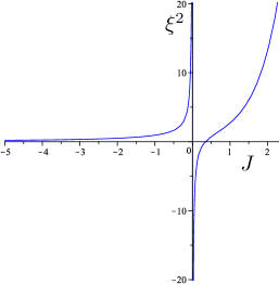
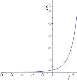
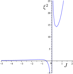
Figure 1: The dependence of the function $\tilde{g}(J,c)$, which is equal to $\xi^{2}$, on $J$ at $c=1/2$ (left), $c=1$ (center) and $c=3$ (right).

Let us consider a special values of $\xi^{2}$ and $c$, which have been obtained in the SFT inspired cosmological model. From the action for the tachyon in the SFT [38] the following equation has been obtained [39]:

$$(-\xi_{0}^{2}\tilde{\alpha}^{2}+1)=3e^{-\tilde{\alpha}^{2}/4},$$ (62)

where

$$\xi_{0}^{2}={}-\frac{1}{4\ln\left(\frac{4}{3\sqrt{3}}\right)}\approx 0.9556.$$ (63)

Substituting $J=-\tilde{\alpha}^{2}/8$, we obtain $\mathcal{F}_{SFT}$ with $\xi_{SFT}^{2}=8\xi_{0}^{2}$ and $c=3$. At $c=3$ we obtain that $\xi^{2}_{1}=0.6080355395$ and $\xi^{2}_{2}=14.16157383$. Therefore, $\xi^{2}_{2}>\xi_{SFT}^{2}>\xi^{2}_{1}$, so there exists no real root at these values of parameters.

4.2 Exact Solution in the Friedmann–Robertson–Walker metric

Let us consider the Einstein equations, which corresponds to a real simple root $J_{1}$ in the Friedmann–Robertson–Walker metric [14]:

$$\left\{\begin{array}[]{l}\displaystyle 3H^{2}=\frac{4\pi G_{N}{\cal F}^{\prime}(J_{1})}{g_{o}^{2}}\left(\dot{\phi}^{2}+J_{1}\phi^{2}\right)+8\pi G_{N}\Lambda,\\[20.48596pt] \displaystyle\dot{H}={}-\frac{4\pi G_{N}{\cal F}^{\prime}(J_{1})}{g_{o}^{2}}\dot{\phi}^{2},\end{array}\right.$$ (64)

where a dot denotes a time derivative.

Exact real solutions of this system have been obtained in [9, 14]. In our notations these solutions are as follows:

At $J_{1}>0$

$$\phi(t)={}\pm\frac{\sqrt{3J_{1}}g_{o}^{2}}{6\pi G_{N}{\cal F}^{\prime}(J_{1})}(t-t_{0}),\qquad H(t)={}-\frac{J_{1}g_{o}^{2}}{6\pi G_{N}{\cal F}^{\prime}(J_{1})}(t-t_{0}),$$ (65)

where $t_{0}$ is an arbitrary constant. These solutions exist only at

$$\Lambda={}-\frac{J_{1}g_{o}^{2}}{24\pi^{2}G_{N}^{2}{\cal F}^{\prime}(J_{1})}\,.$$ (66)

At $J_{1}=0$ summing the first and the second equations of (64), we obtain:

$$\dot{H}=8\pi G_{N}\Lambda-3H^{2}.$$ (67)

The type of solution depends on sign of $\Lambda$:

• $\Lambda=0$

  $$H(t)={}-\frac{1}{3(t-t_{0})},\quad\phi(t)={\tilde{C}}_{1}\pm\frac{\sqrt{3}g_{o}}{\sqrt{\pi G_{N}{\cal F}^{\prime}(0)}}\ln(t-t_{0}),$$ (68)

  where $t_{0}$ and ${\tilde{C}}_{1}$ are arbitrary constants.

• If $\Lambda>0$, then we obtain solutions:

  $$H_{1}(t)=\frac{2\sqrt{6\pi G_{N}\Lambda}}{3}\tanh\left(2\sqrt{6\pi G_{N}\Lambda}(t-t_{0})\right),$$ (69)

  $$\phi_{1}(t)=\pm\sqrt{\frac{{}-g_{o}^{2}}{12\pi G_{N}{\cal F}^{\prime}(0)}}\arctan\left(\sinh\left(2\sqrt{6\pi G_{N}\Lambda}(t-t_{0})\right)\right)+{\tilde{C}}_{2}$$ (70)

  and

  $$\tilde{H}_{1}(t)=\frac{2\sqrt{6\pi G_{N}\Lambda}}{3}\coth\left(2\sqrt{6\pi G_{N}\Lambda}(t-t_{0})\right),$$ (71)

  $$\tilde{\phi}_{1}(t)=\pm\sqrt{\frac{g_{o}^{2}}{12\pi G_{N}{\cal F}^{\prime}(0)}}\ln\left(\tanh\left(\sqrt{6\pi G_{N}\Lambda}\left(t-t_{0}\right)\right)\right)+{\tilde{C}}_{2},$$ (72)

  hereafter $t_{0}$ and ${\tilde{C}}_{2}$ are arbitrary real constants.

• In the case $\Lambda<0$ we obtain the following real solution:

  $$H_{2}(t)={}-\frac{2\sqrt{-6\pi G_{N}\Lambda}}{3}\tan\left(2\sqrt{-6\pi G_{N}\Lambda}(t-t_{0})\right),$$ (73)

  $$\phi_{2}(t)={}\pm\sqrt{\frac{g_{o}^{2}}{12\pi G_{N}{\cal F}^{\prime}(0)}}\mathrm{arctanh}\left(\sin\left(2\sqrt{-6\pi G_{N}\Lambda}(t-t_{0})\right)\right)+{\tilde{C}}_{2}.$$ (74)

The stability of the exact solutions, obtained in the Friedmann–Robertson–Walker metric [14], has been analysed in [40].

4.3 Exact solutions in the Bianchi I metric

In Bianchi I metric with the interval

$${ds}^{2}={}-{dt}^{2}+a_{1}^{2}(t)dx_{1}^{2}+a_{2}^{2}(t)dx_{2}^{2}+a_{3}^{2}(t)dx_{3}^{2},$$ (75)

the Einstein equations, which correspond to the simple root $J=0$ have the following form:

$$H_{1}H_{2}+H_{1}H_{3}+H_{2}H_{3}=8\pi G_{N}\left(\frac{\mathcal{F}^{\prime}(0)}{2g_{o}^{2}}\dot{\phi}^{2}+\Lambda\right),$$ (76)

$$\dot{H}_{2}+H_{2}^{2}+\dot{H}_{3}+H_{3}^{2}+H_{2}H_{3}={}-8\pi G_{N}\left(\frac{\mathcal{F}^{\prime}(0)}{2g_{o}^{2}}\dot{\phi}^{2}-\Lambda\right),$$ (77)

$$\dot{H}_{1}+H_{1}^{2}+\dot{H}_{2}+H_{2}^{2}+H_{1}H_{2}={}-8\pi G_{N}\left(\frac{\mathcal{F}^{\prime}(0)}{2g_{o}^{2}}\dot{\phi}^{2}-\Lambda\right),$$ (78)

$$\dot{H}_{1}+H_{1}^{2}+\dot{H}_{3}+H_{3}^{2}+H_{1}H_{3}={}-8\pi G_{N}\left(\frac{\mathcal{F}^{\prime}(0)}{2g_{o}^{2}}\dot{\phi}^{2}-\Lambda\right),$$ (79)

where $H_{k}\equiv\dot{a}_{k}/a_{k}$, $k=1,2,3$. Note that $\mathcal{F}^{\prime}(0)\neq 0$.

Our goal is to find exact solutions to system (76)–(79). Of course, there exist isotropic solutions, which coincide with exact solutions in the Friedmann–Robertson–Walker metric. For those solutions $H_{1}(t)=H_{2}(t)=H_{3}(t)$. At the same time exact anisotropic solutions do exist.

For $\Lambda=0$ we obtain the following solution:

$$H_{1}(t)=\frac{\tilde{C}_{2}+\tilde{C}_{1}+1}{\tilde{C}_{2}(t-t_{0})},\quad H_{2}(t)={}-\frac{\tilde{C}_{1}}{\tilde{C}_{2}(t-t_{0})},\quad H_{3}(t)={}-\frac{1}{\tilde{C}_{2}(t-t_{0})}\,,$$ (80)

$$\phi(t)={}\pm\frac{\sqrt{-\pi G_{N}\mathcal{F}^{\prime}(0)\left({\tilde{C}}_{1}{\tilde{C}}_{2}+{\tilde{C}}_{1}^{2}+{\tilde{C}}_{1}+{\tilde{C}}_{2}+1\right)}}{4\pi G_{N}g_{o}\mathcal{F}^{\prime}(0){\tilde{C}}_{2}}\ln\left({\tilde{C}}_{2}(t-t_{0})^{2}\right)+{\tilde{C}}_{3},$$ (81)

where ${\tilde{C}}_{1}$, ${\tilde{C}}_{2}$, ${\tilde{C}}_{3}$, and $t_{0}$ are arbitrary constants.

For $\mathcal{F}^{\prime}(0)<0$ we obtain that $\phi(t)$ is a real function at

$${\tilde{C}}_{1}\geqslant-1,\quad{\tilde{C}}_{2}>0\quad\mbox{or}\quad{\tilde{C}}_{1}<-1,\quad{}-\frac{{\tilde{C}}_{1}^{2}+{\tilde{C}}_{1}+1}{{\tilde{C}}_{1}+1}>{\tilde{C}}_{2}>0.$$ (82)

For $\mathcal{F}^{\prime}(0)>0$ we obtain that $\phi(t)$ is a real function at

$${\tilde{C}}_{1}<-1,\qquad{\tilde{C}}_{2}>{}-\frac{{\tilde{C}}_{1}^{2}+{\tilde{C}}_{1}+1}{{\tilde{C}}_{1}+1}.$$

Let us consider the case of $\Lambda=1/(8\pi G_{N})$. There exist not only the following isotropic solution

$$H_{1}(t)=H_{2}(t)=H_{3}(t)=\frac{1}{\sqrt{3}}\tanh\left(\sqrt{3}(t-t_{0})\right),$$ (83)

but also an anisotropic one

$$\begin{split}H_{1}(t)&=\frac{1}{\sqrt{3}}\tanh\left(\frac{\sqrt{3}}{2}(t-t_{0})\right),\\ H_{2}(t)&=\frac{1}{\sqrt{3}}\coth\left(\frac{\sqrt{3}}{2}(t-t_{0})\right),\\ H_{3}(t)&=\frac{1}{2\sqrt{3}}\left(\tanh\left(\frac{\sqrt{3}}{2}(t-t_{0})\right)+\coth\left(\frac{\sqrt{3}}{2}(t-t_{0})\right)\right).\end{split}$$ (84)

The corresponding scalar field is real at $\mathcal{F}^{\prime}(0)>0$ and is equal to

$$\tilde{\phi}(t)={\tilde{C}}_{4}\pm\frac{1}{3\sqrt{2\pi G_{N}g_{o}^{2}\mathcal{F}^{\prime}(0)}}\left(\ln\left(e^{\sqrt{3}(t-t_{0})}+1\right)-\ln\left(e^{\frac{\sqrt{3}}{2}(t-t_{0})}-1\right)-\ln\left(e^{\frac{\sqrt{3}}{2}(t-t_{0})}+1\right)\right),$$

where ${\tilde{C}}_{4}$ is an arbitrary real constant.

5 Conclusion

The main result of this paper is the generalization of the algorithm of localization on nonlocal models with linear potentials. This algorithm is proposed for an arbitrary analytic function $\mathcal{F}(\Box_{g})$, which has both simple and double roots. We have proved that the same functions solve the initial nonlocal Einstein equations and the obtained local Einstein equations. We have found the corresponding local actions and proved the self-consistence of our approach.

It is interesting to consider nonlocal models with an arbitrary analytic $\mathcal{F}(\Box_{g})$, without any restrictions on order of roots. The consideration of simple and double roots allows us to make the conjecture that the existence of local actions, which correspond to a nonlocal action, does not depend on order of $\mathcal{F}(\Box_{g})$ roots and the method of finding particular solutions of the nonlocal Einstein equations can be generalized on a nonlocal action with an arbitrary analytic $\mathcal{F}(\Box_{g})$.

In the case of simple roots exact solutions in the Friedmann–Robertson–Walker metric have been found in [14] (their stability is considered in [40]). In this paper we present exact solutions in Friedmann–Robertson–Walker and Bianchi I metrics. The algorithm of localization does not depend on metric, so it can be used to find solutions in other metrics. For example, the well-known Fisher solutions [41] (see also [42, 43]), which are static spherically symmetric solutions for gravitational system with a massless scalar field, are solutions of the nonlocal Einstein equations (12)–(13) for any $\mathcal{F}(J)$, which has a simple root $J_{0}=0$.

References

-
[1]
K. Ohmori, A Review on Tachyon Condensation in Open String Field Theories,
hep-th/0102085;
I.Ya. Aref’eva, D.M. Belov, A.A. Giryavets, A.S. Koshelev and P.B. Medvedev, Noncommutative Field Theories and (Super)String Field Theories, hep-th/0111208;
W. Taylor, Lectures on D-branes, tachyon condensation, and string field theory, hep-th/0301094 -
[2]
L. Brekke, P.G.O. Freund, M. Olson, and E. Witten,
Nonarchimedean
String Dynamics, Nucl. Phys. B 302 (1988) 365–402;
P.H. Frampton, Ya. Okada, Effective Scalar Field Theory of -Adic String, Phys. Rev. D 37 (1988) 3077–3079;
V.S. Vladimirov, I.V. Volovich, E.I. Zelenov, -adic Analysis and Mathematical Physics, WSP, Singapore, 1994;
B. Dragovich, A.Yu. Khrennikov, S.V. Kozyrev, I.V. Volovich, -Adic Mathematical Physics, Anal. Appl. 1 (2009) 1–17, arXiv:0904.4205 -
[3]
I.Ya. Aref’eva, Nonlocal String Tachyon as
a Model for Cosmological Dark Energy, AIP Conf. Proc. 826,
p-Adic Mathematical Physics, eds. A.Yu. Khrennikov,
Z. Raki c, I.V. Volovich, AIP, Melville, NY, 2006, pp. 301–311; astro-ph/0410443;
I.Ya. Aref’eva, D-brane as a Model for Cosmological Dark Energy, in: ”Contents and Structures of the Universe”, eds. C. Magneville, R. Ansari, J. Dumarchez, and J.T.T. Van, Proc. of the XLIst Rencontres de Moriond, 2006, pp. 131–135;
I.Ya. Aref’eva, Stringy Model of Cosmological Dark Energy, AIP Conf. Proc. 957, Particles, Strings, and Cosmology, eds. A. Rajantie, P. Dauncey, C. Contaldi, H. Stoica, AIP, Melville, NY, 2007, pp. 297–300, arXiv:0710.3017 - [4] I.Ya. Aref’eva and L.V. Joukovskaya, Time Lumps in Nonlocal Stringy Models and Cosmological Applications, JHEP 0510 (2005) 087, hep-th/0504200
- [5] G. Calcagni, Cosmological tachyon from cubic string field theory, JHEP 0605 (2006) 012, hep-th/0512259
-
[6]
N. Barnaby, T. Biswas, and J.M. Cline,
p-adic Inflation, JHEP 0704 (2007) 056,
hep-th/0612230
N. Barnaby and J.M. Cline, Large Nongaussianity from Nonlocal Inflation, JCAP 0707 (2007) 017, arXiv:0704.3426
N. Barnaby, Nonlocal Inflation, Can. J. Phys. 87 (2009) 189–194, arXiv:0811.0814 - [7] A.S. Koshelev, Non-local SFT Tachyon and Cosmology, JHEP 0704 (2007) 029, hep-th/0701103
- [8] I.Ya. Aref’eva, L.V. Joukovskaya, and S.Yu. Vernov, Bouncing and accelerating solutions in nonlocal stringy models JHEP 0707 (2007) 087, hep-th/0701184
- [9] I.Ya. Aref’eva and I.V. Volovich, Quantization of the Riemann Zeta-Function and Cosmology, Int. J. of Geom. Meth. Mod. Phys. 4 (2007) 881–895, hep-th/0701284
- [10] J.E. Lidsey, Stretching the Inflaton Potential with Kinetic Energy, Phys. Rev. D 76 (2007) 043511, hep-th/0703007
-
[11]
G. Calcagni, M. Montobbio, and G. Nardelli, A route to
nonlocal cosmology, Phys. Rev. D 76 (2007) 126001,
arXiv:0705.3043
G. Calcagni and G. Nardelli, Tachyon solutions in boundary and cubic string field theory, Phys. Rev. D 78 (2008) 126010, arXiv:0708.0366;
G. Calcagni, M. Montobbio, and G. Nardelli, Localization of nonlocal theories, Phys. Lett. B 662 (2008) 285–289, arXiv:0712.2237;
G. Calcagni and G. Nardelli, Nonlocal instantons and solitons in string models, Phys. Lett. B 669 (2008) 102–112, arXiv:0802.4395 -
[12]
L.V. Joukovskaya, Dynamics in nonlocal cosmological models derived from string field theory
Phys. Rev. D 76 (2007) 105007, arXiv:0707.1545;
L.V. Joukovskaya, Rolling tachyon in nonlocal cosmology, L.V. Joukovskaya, AIP Conf. Proc. 957, Particles, Strings, and Cosmology, eds. A. Rajantie, P. Dauncey, C. Contaldi, H. Stoica, AIP, Melville, NY, 2007, pp. 325–328, arXiv:0710.0404;
L.V. Joukovskaya, Dynamics with Infinitely Many Time Derivatives in Friedmann–Robertson–Walker Background and Rolling Tachyon, JHEP 0902 (2009) 045, arXiv:0807.2065 - [13] N. Barnaby and N. Kamran, Dynamics with Infinitely Many Derivatives: The Initial Value Problem, JHEP 0802 (2008) 008, arXiv:0709.3968
- [14] I.Ya. Aref’eva, L.V. Joukovskaya, and S.Yu. Vernov, Dynamics in nonlocal linear models in the Friedmann–Robertson–Walker metric, J. Phys. A: Math. Theor. 41 (2008) 304003, arXiv:0711.1364
- [15] S.Yu. Vernov, Exact Solutions in Nonlocal Linear Models, Proc. the Int. Workshop SQS’07, (Dubna, Russia, July 30 - August 4, 2007), eds. E. Ivanov, S. Fedoruk, JINR, Dubna, Russia, 2008, pp. 118–121, arXiv:0802.3324
-
[16]
D.J. Mulryne and N.J. Nunes, Diffusing non-local inflation: Solving
the field equations as an initial value problem,
Phys. Rev. D 78 (2008) 063519, arXiv:0805.0449;
D.J. Mulryne and N.J. Nunes, Non-linear non-local Cosmology, AIP Conf. Proc. 1115 The Dark Side of the Universe, eds. Sh. Khalil, AIP, Melville, NY, 2009, pp. 329–334, arXiv:0810.5471 - [17] N. Barnaby and N. Kamran, Dynamics with Infinitely Many Derivatives: Variable Coefficient Equations, JHEP 0812 (2008) 022, arXiv:0809.4513
- [18] A.S. Koshelev and S.Yu. Vernov, Cosmological perturbations in SFT inspired non-local scalar field models, arXiv:0903.5176
- [19] G. Calcagni and G. Nardelli, Cosmological rolling solutions of nonlocal theories, Int. J. Mod. Phys. D 19 (2010) 329–338, arXiv:0904.4245
- [20] S.Yu. Vernov, Localization of nonlocal cosmological models with quadratic potentials in the case of double roots, Class. Quant. Grav. 27 (2010) 035006, arXiv:0907.0468
- [21] A.S. Koshelev, SFT non-locality in cosmology: solutions, perturbations and observational evidences, arXiv:0912.5457
- [22] I.Ya. Aref’eva and I.V. Volovich, On the null energy condition and cosmology, Theor. Math. Phys. 155 (2008) 503–511 [Teor. Mat. Fiz. 155 (2008) 3–12], hep-th/0612098
- [23] R. Kallosh, J.U. Kang, A. Linde, and V. Mukhanov, The New Ekpyrotic Ghost, JCAP 0804 (2008) 018, arXiv:0712.2040
-
[24]
S. Weinberg,
Effective Field Theory for Inflation,
Phys. Rev. D 77 (2008) 123541,
arXiv:0804.4291;
J.Z. Simon, Higher derivative Lagrangians, non-locality, problems and solutions, Phys. Rev. D 41 (1990) 3720–3733 - [25] P. Creminelli, G. D’Amico, J. Norena, and F. Vernizzi, The Effective Theory of Quintessence: the Side Unveiled, JCAP 0902 (2009) 018, arXiv:0811.0827
-
[26]
A.G. Riess et al. [Supernova Search Team collaboration],
Type Ia Supernova Discoveries at From the Hubble Space
Telescope: Evidence for Past Deceleration and Constraints on Dark
Energy Evolution, Astrophys. J. 607 (2004) 665–687, astro-ph/0402512;
M. Tegmark et al. [SDSS collaboration], The 3D power spectrum of galaxies from the SDS, Astroph. J. 606 (2004) 702–740, astro-ph/0310725;
P. Astier et al., The Supernova Legacy Survey: Measurement of , and from the First Year Data Set, Astron. Astrophys. 447 (2006) 31–48, astro-ph/0510447;
Shirley Ho, Chr. M. Hirata, N. Padmanabhan, U. Seljak, N. Bahcall, Correlation of CMB with large-scale structure: I. ISW Tomography and Cosmological Implications, Phys. Rev. D 78 (2008) 043519, arXiv:0801.0642;
W.M. Wood-Vasey et al. [ESSENCE Collaboration], Observational Constraints on the Nature of the Dark Energy: First Cosmological Results from the ESSENCE Supernova Survey, Astrophys. J. 666 (2007) 694–715, astro-ph/0701041;
D. Baumann et al. [CMBPol Study Team Collaboration], CMBPol Mission Concept Study: Probing Inflation with CMB Polarization, AIP Conf. Proc. 1141, CMB Polarization workshop: theory and foregrounds: CMBPol mission concept, eds. S. Dodelson, D. Baumann et al., AIP, Melville, NY, 2009, pp. 10–120, arXiv:0811.3919;
E. Komatsu, J. Dunkley, M.R. Nolta, C.L. Bennett, B. Gold, G. Hinshaw, N. Jarosik, D. Larson, M. Limon, L. Page, D.N. Spergel, M. Halpern, R.S. Hill, A. Kogut, S.S. Meyer, G.S. Tucker, J.L. Weiland, E. Wollack, E.L. Wright, Five-Year Wilkinson Microwave Anisotropy Probe (WMAP) Observations: Cosmological Interpretation, Astrophys. J. Suppl. 180 (2009) 330–376, arXiv:0803.0547;
M. Kilbinger, K. Benabed, J. Guy, P. Astier, I. Tereno, L. Fu, D. Wraith, J. Coupon, Y. Mellier, C. Balland, F.R. Bouchet, T. Hamana, D. Hardin, H.J. McCracken, R. Pain, N. Regnault, M. Schultheis, and H. Yahagi, Dark energy constraints and correlations with systematics from CFHTLS weak lensing, SNLS supernovae Ia and WMAP5, Astron. Astrophys. 497 (2009) 677–688, arXiv:0810.5129 - [27] Jingfei Zhang and Yuan-Xing Gui, Reconstructing quintom from WMAP 5-year observations: Generalized ghost condensate, Commun. Theor. Phys., 54 (2010) 380–388, arXiv:0910.1200
- [28] A. Shafieloo, V. Sahni, A.A. Starobinsky, Is cosmic acceleration slowing down?, Phys. Rev. D 80 (2009) 101301, arXiv:0903.5141
-
[29]
Yi-Fu Cai, E.N. Saridakis, M.R. Setare, and Jun-Qing Xia,
Quintom Cosmology: theoretical implications and observations, Phys. Rep. 493 (2010) 1–60,
arXiv:0909.2776;
Hongsheng Zhang, Crossing the phantom divide, arXiv:0909.3013 -
[30]
F. Quevedo, Lectures on string/brane cosmology,
Class. Quant. Grav. 19 (2002) 5721–5779, hep-th/0210292;
U.H. Danielsson, Lectures on string theory and cosmology, Class. Quant. Grav. 22 (2005) S1-S40, hep-th/0409274;
M. Trodden and S.M. Carroll, TASI Lectures: Introduction to Cosmology, astro-ph/0401547;
A. Linde, Inflation and String Cosmology, J. Phys. Conf. Ser. 24 (2005) 151–160, hep-th/0503195;
C.P. Burgess, Strings, Branes and Cosmology: What can we hope to learn?, hep-th/0606020;
J.M. Cline, String Cosmology, hep-th/0612129;
L. McAllister and E. Silverstein, String Cosmology: A Review, Gen. Rel. Grav. 40 (2008) 565–605, arXiv:0710.2951 -
[31]
N. Arkani-Hamed, S. Dimopoulos, G. Dvali, and G. Gabadadze,
Nonlocal modification of gravity and the cosmological constant
problem, hep-th/0209227;
A.O. Barvinsky, Nonlocal action for long-distance modifications of gravity theory, Phys. Lett. B 572 (2003) 109–116, hep-th/0304229;
S. Deser and R.P. Woodard, Nonlocal Cosmology, Phys. Rev. Lett. 99 (2007) 111301, arXiv:0706.2151;
S. Nojiri and S.D. Odintsov, Modified non-local- gravity as the key for the inflation and dark energy, Phys. Lett. B 659 (2008) 821–826, arXiv:0708.0924;
S. Jhingan, S. Nojiri, S.D. Odintsov, M. Sami, I Thongkool, and S. Zerbini, Phantom and non-phantom dark energy: The cosmological relevance of non-locally corrected gravity, Phys. Lett. B 663 (2008) 424–428, arXiv:0803.2613;
S. Capozziello, E. Elizalde, Sh. Nojiri, and S.D. Odintsov, Accelerating cosmologies from non-local higher-derivative gravity, Phys. Lett. B 671 (2009) 193–198, arXiv:0809.1535;
T.S. Koivisto, Newtonian limit of nonlocal cosmology, Phys. Rev. D 78 (2008) 123505, arXiv:0807.3778;
S. Capozziello, E. Elizalde, Sh. Nojiri, and S.D. Odintsov, Accelerating cosmologies from non-local higher-derivative gravity, Phys. Lett. B 671 (2009) 193–198, arXiv:0809.1535;
F.W. Hehl and B. Mashhoon, A formal framework for a nonlocal generalization of Einstein’s theory of gravitation, Phys. Rev. D 79 (2009) 064028, arXiv:0902.0560;
S. Nesseris and A. Mazumdar, Newton’s constant in ,) theories of gravity and constraints from BBN, Phys. Rev. D 79 (2009) 104006, arXiv:0902.1185;
C. Deffayet and R.P. Woodard, Reconstructing the Distortion Function for Nonlocal Cosmology, JCAP 0908 (2009) 023, arXiv:0904.0961;
G. Cognola, E. Elizalde, S. Nojiri, S.D. Odintsov, and S. Zerbini, One-loop effective action for non-local modified Gauss-Bonnet gravity in de Sitter space, Eur. Phys. J C 64 (2009) 483–494, arXiv:0905.0543 - [32] A. Pais and G.E. Uhlenbeck, On Field Theories with Nonlocalized Action, Phys. Rev. 79 (1950) 145–165
-
[33]
D.A. Eliezer and R.P. Woodard, The Problem of
Nonlocality in
String Theory, Nucl. Phys. B 325 (1989) 389–469;
J. Llosa and J. Vives, Hamiltonian formalism for nonlocal Lagrangians, J. Math. Phys. 35 (1994) 2856–2877;
R.P. Woodard, A Canonical Formalism For Lagrangians With Nonlocality Of Finite Extent, Phys. Rev. A 62 (2000) 052105;
N. Moeller and B. Zwiebach, Dynamics with Infinitely Many Time Derivatives and Rolling Tachyons, JHEP 0210 (2002) 034, hep-th/0207107;
V.S. Vladimirov and Ya.I. Volovich, Nonlinear Dynamics Equation in p-Adic String Theory, Theor. Math. Phys. 138 (2004) 297–309 [Teor. Mat. Fiz., 138 (2004) 355–368], math-ph/0306018;
A. Sen, Tachyon Dynamics in Open String Theory, Int. J. Mod. Phys. A 20 (2005) 5513–5656, hep-th/0410103
V.S. Vladimirov, On the equation of the -adic open string for the scalar tachyon field, math-ph/0507018;
V. Forini, G. Grignani, and G. Nardelli, A new rolling tachyon solution of cubic string field theory, JHEP 0503 (2005) 079, hep-th/0502151;
L.V. Joukovskaya, Iteration method of solving nonlinear integral equations describing rolling solutions in string theories, Theor. Math. Phys. 146 (2006) 335–342 [Teor. Mat. Fiz. 146 (2006) 402–409], arXiv:0708.0642;
B. Dragovich, Zeta Nonlocal Scalar Fields, Theor. Math. Phys. 157 (2008) 1671–1677 [Teor. Mat. Fiz. 157 (2008) 364–372], arXiv:0804.4114;
G. Calcagni and G. Nardelli, Kinks of open superstring field theory, Nucl. Phys. B 823 (2009) 234–253, arXiv:0904.3744 - [34] H. Yang, Stress tensors in p-adic string theory and truncated OSFT, JHEP 0211 (2002) 007, hep-th/0209197
- [35] I.Ya. Aref’eva, L.V. Joukovskaya, and A.S. Koshelev, Time evolution in superstring field theory on nonBPS brane. 1. Rolling tachyon and energy momentum conservation, JHEP 0309 (2003) 012, hep-th/0301137
-
[36]
H.T. Davis, The Laplace differential equation of infinite
order, Anal. Math. 2 32 (1931) no. 4, 686–714;
H.T. Davis, The Theory of Linear Operators from the Standpoint of Differential Equations of Infinite Order, Indiana, the Principia Press, 1936 -
[37]
R.D. Carmichael, Linear differential equations of infinite
order, Bull. Amer. Math. Soc. 42 (1936) 193–218;
L. Carleson, On infinite differential equations with constant coefficients. I, Math. Scand. 1 (1953) 31–38 - [38] A.Sen and B. Zwiebach, Tachyon condensation in string field theory, JHEP 0003 (2000) 002, hep-th/9912249
- [39] I.Ya. Aref’eva and A.S. Koshelev, Cosmic Acceleration and Crossing of barrier from Cubic Superstring Field Theory, JHEP 0702 (2007) 041, hep-th/0605085
- [40] I.Ya. Aref’eva, N.V. Bulatov, L.V. Joukovskaya, and S.Yu. Vernov, Null Energy Condition Violation and Classical Stability in the Bianchi I Metric, Phys. Rev. D 80 (2009) 083532, arXiv:0903.5264
- [41] I.Z. Fisher, Scalar mesostatic field with regard for gravitational effects, Zh. Eksp. Teor. Fiz. 18 (1948) 636–640, gr-qc/9911008
- [42] K.A. Bronnikov, M.S. Chernakova, J.C. Fabris, N. Pinto-Neto, and M.E. Rodrigues, Cold black holes and conformal continuations, Int. J. Mod. Phys. D 17 (2008) 25–42, gr-qc/0609084
- [43] Sh. Abdolrahimi and A.A. Shoom, Analysis of the Fisher solution, Phys. Rev. D 81 (2010) 024035, arXiv:0911.5380