Reduced fidelity in Kitaev honeycomb model

Abstract

We study reduced fidelity and reduced fidelity susceptibility in the Kitaev honeycomb model. It is shown that the nearest-two-site reduced fidelity susceptibility manifest itself as a peak at the quantum phase transition point, although the one-site reduced fidelity susceptibility vanishes. Our results directly reveal that the reduced fidelity susceptibility can be used to characterize the quantum phase transition in the Kitaev honeycomb model, which suggests that, despite its local nature, the reduced fidelity susceptibility is an accurate marker of the topological phase transition when it is properly chosen.

I introduction

The quantum phase transition (QPT), which is a phase transition driven purely by quantum fluctuations and which occurs at zero temperature, is believed to be an important concept in condensed matter physicscontinuous phase transition ; quantum phase transition . It is defined as the nonanalytic behavior of the ground-state properties, and thus reflects quantum fluctuations, which differentiates it from the temperature-driven thermal phase transition that reflects thermal fluctuations. Most QPTs can be described within the traditional symmetry-breaking formalism; however, there are also exceptions which can only be characterized by topological orderwen-book . In these topological quantum phase transitions (TQPTs), the local perturbation effects may be exponentially suppressed, as was observed in fractional quantum Hall phaseswen-book .

This QPT has appeared in a number of unrealistic models and is also related to many realistic systems such as high temperature superconductorsPALee2006 . Despite many theoretical examples that show the existence of the QPT, there is still no definite way to mark it in terms of a local-order parameter. Recently, much attentionAHamma07 ; DFAbasto08 ; Yang2008 ; JHZhao0803 ; Erik2009 ; Buonsante1 ; TJ2009 ; PZanardi032109 ; PZanardi0701061 ; WLYou07 ; SChen07 ; SJGu072 ; MFYang07 ; NPaunkovic07 has been drawn to the use of fidelity to mark the QPT ( for a review, see Ref. Gurev ). For example, the fidelity approach to the TPQT occurring in the Kitaev toric model have been used in Refs. AHamma07 ; DFAbasto08 , and the fidelity between two states in the Kitaev honeycomb modelKitaev2006 has been studied in Refs. JHZhao0803 ; Yang2008 . E. Eriksson and H. Johannesson proposed that several TQPTs were accurately signaled by a singularity in the second-order derivative of the reduced fidelityErik2009 . Fidelity is suggested to be particularly suited for revealing a QPT in the Bose-Hubbard modelBuonsante1 . Moreover, the ground-state fidelity and various correlations to gauge the competition between different orders in strong correlated system were also discussedTJ2009 .

Fidelity is a concept borrowed from quantum-information theory and is defined as a measure of similarity between two quantum states. Intuitively, it would be a good marker, since the structure of the ground state should suffer a dramatic change through the phase transition point. As fidelity is purely a quantum-information concept, the advantage of using fidelity is that no $a$ $priori$ knowledge of any order parameter and changes of symmetry of the system need to be assumed. This idea has been used to analyze the QPT, and its validity has been confirmed in many systemsGurev .

Meanwhile, the role of the leading term of fidelity was explored PZanardi0701061 ; WLYou07 . The fidelity susceptibility, which is the second derivative of the fidelity with respect to the driving parameter, was introduced to study the QPTWLYou07 . It has been pointed out that the fidelity susceptibility is actually equivalent to the structure factor (fluctuation) of the driving term in the Hamiltonian on the perturbation level. In this case, if the temperature is chosen as the driving parameter of thermal phase transitions, the fidelity susceptibility, which is extracted from the mixed-state fidelity between two thermal statesWXG , is simply the specific heat. From this point of view, using the fidelity to deal with the QPT seems still to be within the framework of the correlation function approach, which is intrinsically related to the local order parameter. Except for the global fidelity, which measures the difference between ground states differing slightly in the driving parameter, the reduced fidelity, which describes the difference of the mix-state of only a local region of the system of interest, was also introduced. It has been demonstrated that the reduced fidelity should be useful in many ordinary symmetry-breaking QPTs as well as some TQPTsErik2009 ; WXG ; Xiong2009 . The reduced fidelity reveals information about a change in the inner structure for a system undergoes a QPT, and it is significant to investigate the behavior of the reduced fidelity susceptibility in both critical and noncritical regions. Recently, it was shown that the TQPT in the Kitaev spin model can be characterized by nonlocal-string order parametersFeng2007 ; Chen2008 ; You2009 , so it would be interesting to see whether it is able to mark this TQPT with a local quantity; namely, the reduced fidelity.

In this work, we study the reduced fidelity and reduced fidelity susceptibility in the Kitaev honeycomb model. Because of its potential application in topological quantum computation, such a model has been the focus of research in recent years, despite its being rather artificialKitaev2006 ; Wen2003 ; RMP2008 ; Schmidt2008 ; You2009 ; Nussinov2009 . We show that the reduced fidelity susceptibility of two nearest sites manifest itself as a peak at the QPT point, although the one-site reduced fidelity susceptibility vanishes. Our results directly reveal that the reduced fidelity susceptibility can be used to characterize the QPT in the Kitaev honeycomb model, and thus suggest that the reduced fidelity susceptibility is an accurate marker of the TQPT when it is properly chosen, despite its local nature.

This article is organized as follows. The model and the calculation of reduced fidelity are presented in Sec. II. The results of the reduced fidelity and fidelity susceptibility are discussed in Sec. III. A summary is given in Sec. IV.

II Reduced fidelity and fidelity susceptibility

The Kitaev honeycomb model was first introduced by Kitaev to study the topological order and anyonic statistics, which describe a honeycomb lattice system with a spin 1/2 located at each site. The Hamiltonian consists of an anisotropic nearest-site interaction with three types of bonds: $J_{x}$, $J_{y}$, and $J_{z}$. The model Hamiltonian is

$$H = -J_{x}\sum_{x\text{-bonds}}\sigma_{j}^{x}\sigma_{k}^{x}-J_{y}\sum_{y\text{-bonds}}\sigma_{j}^{y}\sigma_{k}^{y}-J_{z}\sum_{z\text{-bonds}}\sigma_{j}^{z}\sigma_{k}^{z}$$ (1)

$$= -J_{x}H_{x}-J_{y}H_{y}-J_{z}H_{z},$$

where $j$ and $k$ denote the two ends of the corresponding bond, and $J_{\alpha}$ and $\sigma^{\alpha}(a=x,y,z)$ are dimensionless coupling constants and Pauli matrices respectively.

Bellow, we solve this model within the method developed by KitaevKitaev2006 . Here, we would like to mention that Z. Nussinov and G. Ortiz have also illustrated how Kitaev’s honeycomb model may be solved directlyNussinov2009 . Within this approach, the above Hamiltonian can be rewritten using fermionic operators as

$$H=\sum_{\mathbf{q}}\sqrt{\epsilon_{\mathbf{q}}^{2}+\Delta_{\mathbf{q}}^{2}}\left(C_{\mathbf{q},1}^{{\dagger}}C_{\mathbf{q},1}-C_{\mathbf{q},2}^{{\dagger}}C_{\mathbf{q},2}\right).$$ (2)

with

$$\epsilon_{\mathbf{q}} = J_{x}\cos q_{x}+J_{y}\cos q_{y}+J_{z},$$

$$\Delta_{\mathbf{q}} = J_{x}\sin q_{x}+J_{y}\sin q_{y}.$$ (3)

The momenta take the values

$$q_{x\left(y\right)}=\frac{2n\pi}{L},n=-\frac{L-1}{2},\cdots,\frac{L-1}{2}$$ (4)

where $L$ is an odd integer; then the system size is $N=2L^{2}$.

Therefore, we have the ground state

$$\left|\Psi_{0}\right\rangle=\prod_{\mathbf{q}}C_{\mathbf{q},2}^{{\dagger}}\left|0\right\rangle,$$ (5)

with the ground-state energy

$$E_{0}=-\sum_{\mathbf{q}}\sqrt{\epsilon_{\mathbf{q}}^{2}+\Delta_{\mathbf{q}}^{2}}=-\sum_{\mathbf{q}}E_{\mathbf{q}}.$$ (6)

The two-site reduced density matrix can be expressed as You2009

$$\rho(\mathbf{r}_{1},\mathbf{r}_{2}) = \mathrm{Tr}^{\prime}\left(|g\rangle\langle g|\right)$$ (7)

$$= \frac{1}{4}\sum_{\alpha,\alpha^{\prime}=0}^{3}\left\langle g\left|\sigma_{{1}}^{\alpha}\sigma_{{2}}^{\alpha^{\prime}}\right|g\right\rangle\sigma_{{1}}^{\alpha}\sigma_{{2}}^{\alpha^{\prime}},$$

where $\sigma^{\alpha}$$($$\sigma^{\alpha^{\prime}}$$)$ are Pauli matrices $\sigma^{x}$, $\sigma^{y}$, and $\sigma^{z}$ for $\alpha$ $($$\alpha^{\prime}$$)$$=1$ to 3, and the unit matrix for $\alpha$ $($$\alpha^{\prime}$$)$$=0$.

Now we consider the nearest-two-site reduced density matrix, (i.e., the reduced density matrix of an $x$-bond. It can be proved that all but two parts of the density matrix are nonzero:

$$\rho(\mathbf{r},\mathbf{r+x})\!\!=\!\!\frac{1}{4}\left\langle g\left|\sigma_{\mathbf{r}}^{x}\sigma_{\mathbf{r+x}}^{x}\right|g\right\rangle\sigma_{\mathbf{r}}^{x}\sigma_{\mathbf{r+x}}^{x}\!+\frac{1}{4}I_{\mathbf{r}}I_{\mathbf{r+x}}.$$ (8)

If we assume the system has translational symmetry, we can calculate the average

$$\left\langle g\left|\sigma_{\mathbf{r}}^{x}\sigma_{\mathbf{r+x}}^{x}\right|g\right\rangle=\frac{1}{L^{2}}\left\langle g\left|H_{x}\right|g\right\rangle=-\frac{1}{L^{2}}\frac{\partial E_{0}}{\partial J_{x}}.$$ (9)

Combining Eqs. (6) and (9), the reduced density matrix can be expressed as

$$C_{x} \equiv \left\langle g\left|\sigma_{\mathbf{r}}^{x}\sigma_{\mathbf{r+x}}^{x}\right|g\right\rangle$$ (10)

$$= -\frac{1}{L^{2}}\frac{\partial E_{0}}{\partial J_{x}}$$

$$= \frac{1}{L^{2}}\sum_{\mathbf{q}}\left(\frac{\epsilon_{\mathbf{q}}}{E_{\mathbf{q}}}\cdot\frac{\partial\epsilon_{\mathbf{q}}}{\partial J_{x}}+\frac{\Delta_{\mathbf{q}}}{E_{\mathbf{q}}}\cdot\frac{\partial\Delta_{\mathbf{q}}}{\partial J_{x}}\right)$$

$$= \frac{1}{L^{2}}\sum_{\mathbf{q}}\left(\frac{\epsilon_{\mathbf{q}}\cdot\cos{q_{x}}+\Delta_{\mathbf{q}}\cdot\sin{q_{x}}}{E_{\mathbf{q}}}\right).$$

Similarly, for the $y$ and $z$ bonds, we can also obtain

$$\rho(\mathbf{r},\mathbf{r+y})\! \!=\! \!\frac{1}{4}\left\langle g\left|\sigma_{\mathbf{r}}^{y}\sigma_{\mathbf{r+y}}^{y}\right|g\right\rangle\sigma_{\mathbf{r}}^{y}\sigma_{\mathbf{r+y}}^{y}\!+\frac{1}{4}I_{\mathbf{r}}I_{\mathbf{r+y}},$$

$$\rho(\mathbf{r},\mathbf{r+z})\! \!=\! \!\frac{1}{4}\left\langle g\left|\sigma_{\mathbf{r}}^{z}\sigma_{\mathbf{r+z}}^{z}\right|g\right\rangle\sigma_{\mathbf{r}}^{z}\sigma_{\mathbf{r+z}}^{z}\!+\frac{1}{4}I_{\mathbf{r}}I_{\mathbf{r+z}},$$ (11)

where

$$C_{y} \equiv \left\langle g\left|\sigma_{\mathbf{r}}^{y}\sigma_{\mathbf{r+y}}^{y}\right|g\right\rangle$$

$$= -\frac{1}{L^{2}}\frac{\partial E_{0}}{\partial J_{y}}$$

$$= \frac{1}{L^{2}}\sum_{\mathbf{q}}\left(\frac{\epsilon_{\mathbf{q}}}{E_{\mathbf{q}}}\cdot\frac{\partial\epsilon_{\mathbf{q}}}{\partial J_{y}}+\frac{\Delta_{\mathbf{q}}}{E_{\mathbf{q}}}\cdot\frac{\partial\Delta_{\mathbf{q}}}{\partial J_{y}}\right)$$

$$= \frac{1}{L^{2}}\sum_{\mathbf{q}}\left(\frac{\epsilon_{\mathbf{q}}\cdot\cos{q_{y}}+\Delta_{\mathbf{q}}\cdot\sin{q_{y}}}{E_{\mathbf{q}}}\right),$$

$$C_{z} \equiv \left\langle g\left|\sigma_{\mathbf{r}}^{z}\sigma_{\mathbf{r+z}}^{z}\right|g\right\rangle$$ (12)

$$= -\frac{1}{L^{2}}\frac{\partial E_{0}}{\partial J_{z}}$$

$$= \frac{1}{L^{2}}\sum_{\mathbf{q}}\left(\frac{\epsilon_{\mathbf{q}}}{E_{\mathbf{q}}}\cdot\frac{\partial\epsilon_{\mathbf{q}}}{\partial J_{z}}+\frac{\Delta_{\mathbf{q}}}{E_{\mathbf{q}}}\cdot\frac{\partial\Delta_{\mathbf{q}}}{\partial J_{z}}\right)$$

$$= \frac{1}{L^{2}}\sum_{\mathbf{q}}\left(\frac{\epsilon_{\mathbf{q}}}{E_{\mathbf{q}}}\right).$$

After arriving at a diagonal reduced density matrix, it is easy and straightforward to calculate the reduced fidelity

$$F=\sum_{i}\sqrt{\rho_{ii}\rho^{\prime}_{ii}}.$$ (13)

Thus we have the expression

$$F_{\alpha} = \frac{1}{2}[(1+C_{\alpha})(1+C^{\prime}_{\alpha})+(1-C_{\alpha})(1-C^{\prime}_{\alpha})],$$ (14)

where $C_{\alpha}$ are $C_{x}$, $C_{y}$, and $C_{z}$ for $x$, $y$, and $z$ bond, respectively, and $F_{\alpha}$ are $F_{x}$, $F_{y}$, and $F_{z}$.

Now we calculate the reduced fidelity susceptibility $\chi_{F}$. For diagonal density matrices, the fidelity susceptibility is

$$\chi_{F}=\sum_{i}\frac{(\partial_{J_{\alpha}}\rho_{ii})^{2}}{4\rho_{ii}}=\sum_{i}\frac{(\partial_{J_{s}}C_{\alpha})^{2}}{4\rho_{ii}},$$ (15)

where $J_{s}$ is the driving parameter.

With this expression, we first set $J_{x}=J_{y}$ and select $J_{z}$ as the driving parameter, and then we have

$$\epsilon_{\mathbf{q}} = \frac{1-J_{z}}{2}\cos q_{x}+\frac{1-J_{z}}{2}\cos q_{y}+J_{z},$$

$$\epsilon_{\mathbf{q}}^{\prime} \equiv \frac{\partial\epsilon_{\mathbf{q}}}{\partial J_{z}}=-\frac{1}{2}\cos q_{x}-\frac{1}{2}\cos q_{y}+1,$$

$$\Delta_{\mathbf{q}} = \frac{1-J_{z}}{2}\sin q_{x}+\frac{1-J_{z}}{2}\sin q_{y},$$

$$\Delta_{\mathbf{q}}^{\prime} \equiv \frac{\partial\Delta_{\mathbf{q}}}{\partial J_{z}}=-\frac{1}{2}\sin q_{x}-\frac{1}{2}\sin q_{y},$$

$$E_{\mathbf{q}}^{\prime} \equiv \frac{\partial E_{\mathbf{q}}}{\partial J_{z}}=\frac{\epsilon_{\mathbf{q}}}{E_{\mathbf{q}}}\epsilon_{\mathbf{q}}^{\prime}+\frac{\Delta_{\mathbf{q}}}{E_{\mathbf{q}}}\Delta_{\mathbf{q}}^{\prime},$$ (16)

and

$$\partial_{J_{z}}C_{x} = \frac{1}{L^{2}}\sum_{\mathbf{q}}\frac{1}{E_{\mathbf{q}}^{2}}$$

$$[(E_{\mathbf{q}}\epsilon_{\mathbf{q}}^{\prime}-E_{\mathbf{q}}^{\prime}\epsilon_{\mathbf{q}})\cos q_{x}+(E_{\mathbf{q}}\Delta_{\mathbf{q}}^{\prime}-E_{\mathbf{q}}^{\prime}\Delta_{\mathbf{q}})\sin q_{x}]$$

$$\partial_{J_{z}}C_{y} = \frac{1}{L^{2}}\sum_{\mathbf{q}}\frac{1}{E_{\mathbf{q}}^{2}}$$

$$[(E_{\mathbf{q}}\epsilon_{\mathbf{q}}^{\prime}-E_{\mathbf{q}}^{\prime}\epsilon_{\mathbf{q}})\cos q_{y}+(E_{\mathbf{q}}\Delta_{\mathbf{q}}^{\prime}-E_{\mathbf{q}}^{\prime}\Delta_{\mathbf{q}})\sin q_{y}]$$

$$\partial_{J_{z}}C_{z} = \frac{1}{L^{2}}\sum_{\mathbf{q}}\frac{E_{\mathbf{q}}\epsilon_{\mathbf{q}}^{\prime}-E_{\mathbf{q}}^{\prime}\epsilon_{\mathbf{q}}}{E_{\mathbf{q}}^{2}}.$$ (17)

Also, we can set $J_{z}=1/3$ and make $J_{x}$ the driving parameter, and the formula can be achieved in a similar way. Then, we can study the reduced fidelity and reduced fidelity susceptibility depending on which parameters we are interested in.

III Results and discussions

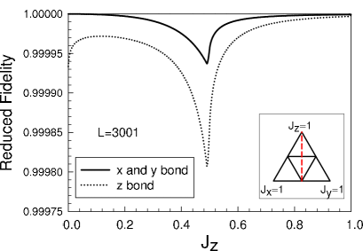
Figure 1: (Color online) Two-site reduced fidelity as a function of $J_{z}$ along the dashed line shown in the triangle for the $x$, $y$ and $z$ bonds.

To study the reduced fidelity susceptibility of the Kitaev honeycomb model, the parameters shall be restricted to the $J_{x}+J_{y}+J_{z}=1$ plane. According to KitaevKitaev2006 , this plane is divided into a gapped phase and a gapless phase. These two phases are separated by the triangle line connecting the $J_{x}=1/2$, $J_{y}=1/2$, and $J_{z}=1/2$ points. As we already arrived at the expression of the reduced fidelity and the reduced fidelity susceptibility, now we begin to calculate these quantities numerically. We start from the nearest-two-site reduced fidelity, since there are three types of nearest sites for a honeycomb lattice. In Figs. 1 and 2, the two-site reduced fidelity with system size $L=3001$ for all three different bonds are shown along two orthogonal parameter directions, $J_{x}=J_{y}$ and $J_{z}=1/3$, which are marked in the inset of the figure. In Fig. 1, the parameter is chosen to be $J_{x}=J_{y}$, and the reduced fidelities are plotted as a function of $J_{z}$, where we can see that the $x$ bond and $y$ bond reduced fidelities are the same, whereas the $z$-bond reduced fidelity differs. In Fig. 2, the parameter is chosen to be $J_{z}=1/3$ and the reduced fidelities are plotted as functions of $J_{x}$, where we can see that the $x-$ and $y-$bond reduced fidelities are symmetric with respect to $J_{x}=1/3$, and the $z-$bond reduced fidelity differs. However, in these two cases, among all three bonds, the reduced fidelity manifests a dip at the phase transition point. It is quite clear that the two-site reduced fidelity can serve as a signature for the TQPT in the Kitaev honeycomb model.

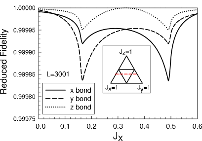
Figure 2: (Color online) Two-site reduced fidelity as a function of $J_{x}$ along the dashed line shown in the triangle for the $x$, $y$, and $z$ bonds.

In order to illustrate the ability of reduced fidelity to mark the TQPT in Kitaev honeycomb model, we calculate the reduced fidelity susceptibility and present the results of the reduced fidelity susceptibility for a system size $L$=3001 and for different bonds along $J_{x}=J_{y}$ and $J_{z}=1/3$ in Fig. 3 and Fig. 4. As expected, the reduced fidelity susceptibility shows a sharp peak at the TPQT point, which would be a clear sign of the phase transition. Comparing with the global fidelity susceptibility, the oscillation in the B phase seems to be missing. Since it has been shown that the oscillating of the global fidelity susceptibility might be related to the long-range correlation function, this disappearance seems to represent the locality of the bond-reduced fidelity susceptibility.

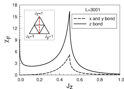
Figure 3: (Color online) Two-site reduced fidelity susceptibility as a function of $J_{z}$ along the dashed line shown in the triangle for $x$, $y$, and $z$ bond.

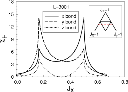
Figure 4: (Color online) Two-site reduced fidelity susceptibility as a function of $J_{x}$ along the dashed line shown in the triangle for $x$, $y$, and $z$ bond.

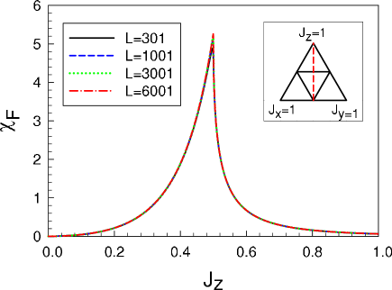
Figure 5: (Color online) $x$-bond two-site reduced fidelity susceptibility as a function of $J_{z}$ along the dashed line shown in the triangle for the various system sizes $L$=301, 1001, 3001, 6001.

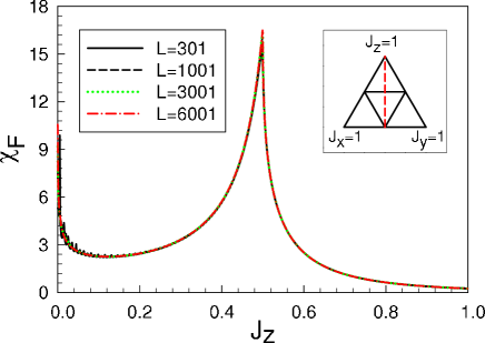
Figure 6: (Color online) $z$-bond two-site reduced fidelity susceptibility as a function of $J_{z}$ along the dashed line shown in the triangle for the various system sizes $L$=301, 1001, 3001, 6001.

To further understand the properties of the reduced fidelity susceptibility, we study its scaling behavior. In Figs. 5-9, the reduced fidelity susceptibility of different bonds at different parameter lines with different system sizes $L$ are presented. Figure 5 ( Fig. 6 ) shows the $x-$bond ( $z-$bond ) two-site reduced fidelity susceptibility as a function of $J_{z}$, and Fig. 8 ( Fig. 9 ) shows the $x-$bond ( $z-$bond ) two-site reduced fidelity susceptibility as a function of $J_{x}$, along the dashed line shown in the triangle for the various system sizes $L$=301, 1001, 3001, 6001. It is obvious that the susceptibility barely changes with increasing lattice number in all the present data.

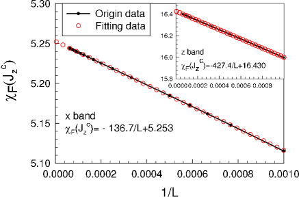
Figure 7: (Color online) $x$-bond two-site reduced fidelity susceptibility as a function of system sizes $L$ at the critical point $J^{c}_{z}$=1/2; dark lines with points indicate numerical data while open red circles indicate the fitting data. Inset: behavior of $z$-bond two-site reduced fidelity susceptibility as a function of the system size $L$ at the critical point $J^{c}_{z}$=1/2.

From Figs. 5 and 6, one may also learn that the peak of reduced fidelity increases slightly as the system sizes $L$ increases around the critical point $J_{z}^{c}$=1/2. To study the scaling behavior of the fidelity susceptibility at the critical point, we perform a finite-size scaling analysis. In Fig. 7, dark lines with points indicate $\chi_{F}(J_{z}^{c})(x)$, the $x-$bond two-site reduced fidelity susceptibility at $J_{z}^{c}$ as a function of system size $L$, and the red circles show the results of fitting data. In the inset, the behavior of $\chi_{F}(J_{z}^{c})(z)$, the $z-$bond two-site reduced fidelity susceptibility at $J_{z}^{c}$ is also shown. The reduced fidelity susceptibility at the critical point depends on the system size, which may be fit as

$$\chi_{F}(J_{z}^{c})(x) \simeq -\frac{136.7}{L}+5.253,$$

$$\chi_{F}(J_{z}^{c})(z) \simeq -\frac{427.4}{L}+16.430.$$ (18)

As shown in Fig. 7, the fitting data agree with the original data rather well, so we may extrapolate $\chi_{F}(J_{z}^{c})$, in the thermodynamic limit. In the thermodynamic limit scales, and for the $x-$bond two-site reduced fidelity susceptibility, $\chi_{F}(J_{z}^{c})$ is $5.253(\pm 0.001)$ , while $\chi_{F}(J_{z}^{c})$ should be $16.430(\pm 0.001)$ for the $z-$bond two-site reduced fidelity susceptibility.

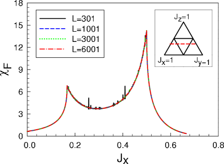
Figure 8: (Color online) $x$-bond two-site reduced fidelity susceptibility as a function of $J_{x}$ along the dashed line shown in the triangle for the various system sizes $L$=301, 1001, 3001, 6001.

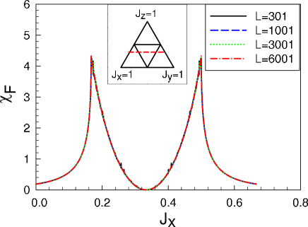
Figure 9: (Color online) $z$-bond two-site reduced fidelity susceptibility as a function of $J_{x}$ along the dashed line shown in the triangle for various system sizes $L$=301, 1001, 3001, 6001.

These results confirm the previous conjecture; namely, that, the divergence of the global fidelity susceptibility is related to long-range correlations. The divergence disappears in the reduce fidelity susceptibility because the reduced fidelity susceptibility averages over all long-range properties and only retains the nearest-site correlation information.

IV summary

In summary, we study the reduced fidelity and reduced fidelity susceptibility in the Kitaev honeycomb model. It is shown that the nearest-two-site reduced fidelity susceptibility manifest itself as a peak at the quantum phase transition point, although the one-site reduced fidelity susceptibility vanishes. Our results directly reveal that the reduced fidelity susceptibility is able to mark the quantum phase transition in the Kitaev honeycomb model, and thus suggest that the reduced fidelity susceptibility is still an accurate marker of the TPQT when it is properly chosen, despite its local nature. The conclusion that such a local quantity can characterize a TQPT is conceptually consistent with the fact that any physical observable is local in nature.

References

• (1) S. L. Sondhi, S. M. Girvin, J. P. Carini, and D. Shahar, Rev. Mod. Phys. 69, 315 (1997).
• (2) S. Sachdev, Quantum Phase Transitions (Cambridge University Press, Cambridge, 1999).
• (3) X. G. Wen, Quantum Field Theory of Many-Body Systems (Oxford University, New York, 2004).
• (4) P. A. Lee, N. Nagaosa, and X. G. Wen, Rev. Mod. Phys. 78, 17 (2006).
• (5) A. Hamma, W. Zhang, S. Haas, and D. A. Lidar, Phys. Rev. B 77, 155111 (2008).
• (6) D. F. Abasto, A. Hamma, and P. Zanardi, Phys. Rev. A 78, 010301(R) (2008).
• (7) S. Yang, S. J. Gu, C. P. Sun and H. Q. Lin, Phys. Rev. A. 78, 012304 (2008).
• (8) J. H. Zhao and H. Q. Zhou, Phys. Rev. B 80, 014403 (2009).
• (9) E. Eriksson and H. Johannesson, Phys. Rev. A 79, 060301 (R) (2009).
• (10) P. Buonsante and A. Vezzani, Phys. Rev. Lett. 98, 110601 (2007).
• (11) M. Rigol, B. S. Shastry and S. Haas, Phys. Rev. B 80, 094529 (2009).
• (12) P. Zanardi, H. T. Quan, X. Wang, and C. P. Sun, Phys. Rev. A 75, 032109 (2007).
• (13) P. Zanardi, P. Giorda, and M. Cozzini, Phys. Rev. Lett. 99, 100603 (2007).
• (14) W. L. You, Y. W. Li, and S. J. Gu, Phys. Rev. E 76, 022101 (2007).
• (15) S. Chen, L. Wang, S. J. Gu, and Y. Wang, Phys. Rev. E 76 061108 (2007); S. Chen, L. Wang, Y. Hao, and Y. Wang, Phys. Rev. A 77 032111 (2008).
• (16) S. J. Gu, H. M. Kwok, W. Q. Ning, and H. Q. Lin, Phys. Rev. B 77, 245109 (2008).
• (17) M. F. Yang, Phys. Rev. B 76, 180403 (R) (2007); Y. C. Tzeng and M. F. Yang, Phys. Rev. A 77, 012311 (2008).
• (18) N. Paunkovic, P. D. Sacramento, P. Nogueira, V. R. Vieira, and V. K. Dugaev, Phys. Rev. A 77, 052302 (2008).
• (19) For a review, see S. J. Gu, e-print arXiv: 0811.3127.
• (20) A. Kitaev, Ann. Phys. (N. Y. ) 303, 2(2003); 321, 2 (2003).
• (21) J. Ma, X. G. Wang, and S. J. Gu, Phys. Rev. E 80, 021124 (2009); J. Ma, L. Xu, H. N. Xiong, and X. G. Wang, Phys. Rev. E 78, 051126 (2008).
• (22) H. N. Xiong, J. Ma, Zhe Sun, and X. G. Wang, Phys. Rev. B 79, 174425 (2009).
• (23) X. Y. Feng, G. M. Zhang, and T. Xiang, Phys. Rev. Lett. 98, 087204 (2007).
• (24) H. D. Chen and Z. Nussinov, J. Phys. A 41, 075001 (2008).
• (25) X. F. Shi, Y. Yu, J. Q. You, and F. Nori, Phys. Rev. B 79, 134431 (2009).
• (26) X. G. Wen, Phys. Rev. Lett. 90, 016803 (2003); M. A. Levin and X. G. Wen, Phys. Rev. B 71,045110 (2005).
• (27) S. D. Sarma, M. Freedman, C. Nayak, S. H. Simon,and A. Stern, Rev. Mod. Phys. 80, 1083 (2008).
• (28) K. P. Schmidt, S. Dusuel, and J. Vidal, Phys. Rev. Lett. 100, 057208 (2008); S. Dusuel, K. P. Schmidt, and J. Vidal, $ibid$. 100, 177204 (2008).
• (29) Z. Nussinov and G. Ortiz, Phys. Rev. B 79, 214440 (2009).