Local observation of antibunching in a trapped Fermi gas

Abstract

Local density fluctuations and density profiles of a Fermi gas are measured in-situ and analyzed. In the quantum degenerate regime, the weakly interacting ⁶Li gas shows a suppression of the density fluctuations compared to the non-degenerate case, where atomic shot noise is observed. This manifestation of antibunching is a direct result of the Pauli principle and constitutes a local probe of quantum degeneracy. We analyze our data using the predictions of the fluctuation-dissipation theorem and the local density approximation, demonstrating a fluctuation-based temperature measurement.

A finite-size system in thermodynamic equilibrium with its surrounding shows characteristic fluctuations, which carry important information about the correlation properties of the system. In a classical gas, fluctuations of the number of atoms contained in a small sub-volume yield a Poisson distribution, reflecting the uncorrelated nature of the gas. An intriguing situation arises when the thermal de Broglie wavelength approaches the interparticle separation and the specific quantum statistics of the constituent particles becomes detectable. For bosons, positive density correlations build up, until Bose-Einstein condensation occurs, as measured in Hanbury Brown-Twiss (HBT) experiments hanbury_brown_test_1956 ; Baym_1998 ; Yasuda_1996 ; altman_probing_2004 ; Oettl_2005 ; folling_spatial_2005 ; schellekens_hanbury_2005 . The effect of bunching also manifests itself in enhanced density fluctuations in real space esteve_observations_2006 . In contrast, fermions obey the Pauli principle. This gives rise to anti-correlations, which have been observed in HBT experiments henny_fermionic_1999 ; oliver_hanbury_1999 ; iannuzzi_direct_2006 ; rom_free_2006 ; jeltes_comparison_2007 , and are expected to squeeze density fluctuations below the classical shot noise limit belzig_2007 . Moreover, for trapped fermions, the reduction of fluctuations varies in space, reaching a maximum in the dense center of the cloud, which should be accessible to a local measurement.

In this letter we report on high-resolution in-situ measurements of density fluctuations in an ultracold Fermi gas of weakly interacting ⁶Li atoms. We extract the mean and the variance of the density profile from a number of absorption images recorded under the same experimental conditions. Our measurements show that the density fluctuations in the center of the trap are suppressed for a quantum degenerate gas as compared to a non-degenerate gas. We analyze our data using the fluctuation-dissipation theorem, which relates the density fluctuations of the gas to its isothermal compressibility. This allows us to extract the temperature of the system zhou_universal_2009 ; esteve_observations_2006 ; gemelke_in_2009 .

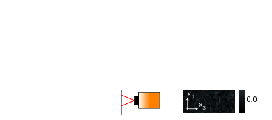
Figure 1: (a) Setup for high-resolution imaging of the trapped ⁶Li gas. The shadow cast by the atoms held in the dipole trap is imaged through the microscope objective and a telephoto objective onto an EMCCD chip. The resolution ($1/e^{2}$-radius) is $1.8\,\mathrm{\mu m}$ depth at a wavelength of $671\,\mathrm{nm}$ and the magnification is $54$. (b) Density distribution (atoms per pixel) of the trapped atoms obtained by averaging over $20$ realizations. The effective pixel size measures $1.2\,\mathrm{\mu m}$ bin , the maximum optical density is $\sim 2$. The images which we evaluate are $\sim 40\,\mathrm{\mu m}$ wide showing the center of the cloud, which has a total length of $500\,\rm{\mu m}$.

We first describe the experimental procedure to obtain a quantum degenerate gas of about $6\times 10^{4}$ ⁶Li atoms equally populating the two lowest hyperfine states. Following the method described in jochim_bose-einstein_2003 , the atoms are loaded into an optical dipole trap created by a far off-resonant laser with a wavelength of $1064\,\mathrm{nm}$, focused to a $1/e^{2}$-radius of $(22\pm 1)\,\mathrm{\mu m}$ errors . The cloud is then optically moved gustavson_transport_2001 into a glass cell that provides high optical access, see Fig. 1(a). In the glass cell, forced evaporation is performed by reducing the trap power from initially $2\,\mathrm{W}$ to $4.7\,\mathrm{mW}$. During evaporation a homogeneous magnetic field of $300\,\mathrm{G}$ is applied to set the s-wave scattering length $a$ for inter-state collisions to $-300\,a_{0}$, where $a_{0}$ is the Bohr radius. The magnetic field is then ramped to $475\,\mathrm{G}$ in $150\,\mathrm{ms}$, changing $a$ to $-100\,a_{0}$, and finally the power of the trapping beam is increased to $10\,{\rm mW}$ in $100\,\mathrm{ms}$. Alternatively, we prepare the lithium gas at temperatures above quantum degeneracy. For this, we evaporate to $50\,{\rm mW}$ before recompressing to $100\,{\rm mW}$, followed by a $100\,{\rm ms}$ period of parametric heating. In both cases, the cloud is allowed to thermalize for $350\,\mathrm{ms}$ before an absorption image is taken. The gas is weakly interacting since $|k_{F}a|<10^{-2}$, with $k_{F}$ the Fermi wavevector.

Our imaging setup is sketched in Fig. 1(a). The probe light, resonant with the lowest hyperfine state of the $|2S_{1/2}\rangle$ to $|2P_{3/2}\rangle$ transition, is collected by a high-resolution microscope objective and imaged on an electron-multiplying CCD (EMCCD) chip. The atoms are illuminated for $8\,{\rm\mu s}$, each atom scattering about 20 photons on average. Fig. 1(b) shows the average density distribution obtained in $20$ experiments.

We now present our procedure for extracting the spatially resolved variance of the atomic density. The position of each pixel in the imaging plane of the camera defines a line of sight intersecting with the atomic cloud. Correspondingly, each pixel bin , having an effective area $A$, determines an observation volume in the atomic cloud along this line of sight. At low saturation, the transmission $t$ of the probe light through an observation volume containing $N$ atoms reads $t=e^{-\sigma\cdot N/A}$, where $\sigma$ is the photon absorption cross section. As a consequence, for small Gaussian fluctuations of the atom number, the relative fluctuations of the transmission coefficient are equal to the absolute fluctuations of the optical density and are thus directly proportional to the number fluctuations:

$$\frac{\delta t^{2}}{\langle t\rangle^{2}}=\frac{\sigma^{2}}{A^{2}}\delta N^{2},$$ (1)

where $\delta t^{2}$, $\langle t\rangle$ and $\delta N^{2}$ are the variance and the mean of the transmission coefficient, and the variance of atom number, respectively.

Experimentally, repeated measurements of identically prepared clouds provide us with a set of count numbers $C$ for each pixel, i.e. each observation volume, corresponding to a certain number of incoming photons registered by the EMCCD. Typically we register $\sim 1300$ counts, corresponding to $\sim 130$ photons at the position of the atoms. We then compute the variance $\delta C^{2}$ and mean $\langle C\rangle$. The relative noise of the counts and the relative noise of the transmission are related by:

$$\frac{\delta C^{2}}{\langle C\rangle^{2}}=\frac{2g}{\langle C\rangle}+\frac{\delta t^{2}}{\langle t\rangle^{2}}.$$ (2)

Here, $g$ is the gain of the camera for converting photoelectrons to counts. The first term is the contribution of photon shot noise while the second term is the contribution of atomic noise. The factor $2$ in the photon shot noise term is caused by the electron-multiplying register basden_photon_2003 . We extract the contribution of the atoms to the relative fluctuations of the counts, by subtracting photon shot noise on each pixel according to (2). This requires the value of $g$ (typically $\sim 15$), which we determine from the linear relationship between the variance and the mean of the number of counts in a set of repeated measurements. The atom number fluctuations are subsequently obtained from (1). At this stage no division by a reference image has been performed, avoiding this source of noise.

To reduce technical noise adding to these fluctuations, we reject images showing the largest deviations of total atom number or cloud position post , which amounts to excluding about $30\%$ of the images. The remaining shot-to-shot fluctuations of the total atom number $\delta N_{\rm tot}^{2}$ are taken into account by further subtracting the quantity $\delta N_{\rm tot}^{2}/N_{\rm tot}^{2}\langle N\rangle^{2}$, which is less than $<2\%$ of $N$ esteve_observations_2006 . Total probe intensity variations from shot to shot are below $0.5\,\%$. Applying this algorithm to each pixel of the images yields a local measurement of the variance of the atom number.

The mean atom number per pixel is calculated by dividing the mean transmission profile by the mean of reference images taken without atoms after each shot, thus averaging shot-noise before division. The values for variance and mean, obtained by applying the above procedures, are then averaged along equipotential lines of the trap. These lines deviate from horizontal lines ($x_{3}$-axis) in our images by less than half a pixel ($0.6\,{\rm\mu m}$).

Fig. 2 shows the observed variance of the atom number plotted against the mean atom number detected on a pixel. One set of data was taken for a gas at temperatures above quantum degeneracy (red squares) and another set of data for a quantum degenerate gas (blue circles). Above quantum degeneracy, the observed variance is found to be proportional to the mean number of atoms. The linear behavior confirms that the fluctuations originate from atomic shot noise.

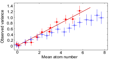
Figure 2: Observed variance versus mean of the atom number detected on a pixel. Red squares show the data for a non-degenerate and blue circles for a quantum degenerate gas. The solid red line is a linear fit to the non-degenerate gas, yielding a slope of $0.20\pm 0.02$. For the data shown, $80$ experiments were performed, $60$ for the degenerate case and $20$ for the non-degenerate case. About 30$\%$ of the experiments were excluded. The error bars shown are estimated from the subtraction of photon shot noise which is the dominant contribution.

To quantitatively understand the slope of the noise curve, which is fitted to be $0.20\pm 0.02$, two main effects have to be considered. These reduce the observed variance and explain the deviation from a slope of one, which would be expected for the full shot noise. First, the effective size of the pixel is of the order of the resolution of the imaging system. As a consequence, the observed noise is the result of a blurring of the signal over the neighboring pixels. This effect is also observed in esteve_observations_2006 ; gemelke_in_2009 , and explains a reduction factor of $0.22$ binsize . Second, the probe light intensity used for the detection is ($15\pm 1)\%$ of the saturation intensity. This leads to a reduction of the photon absorption cross section due to saturation by $0.95$ and due to the Doppler-shift by about $0.9$. Together, these effects lead us to expect a slope of about $0.19$, in good agreement with the observations.

We now turn to the data taken for the quantum degenerate gas (blue circles in Fig. 2). At low densities, the variance is again found to be proportional to the mean density. For increasingly higher densities, we observe a departure from the linear behavior and the density fluctuations are reduced compared to the shot noise limit seen for the non-degenerate gas. This is a direct consequence of the Pauli principle which determines the properties of a quantum degenerate Fermi gas. One can think of the Pauli principle as giving rise to an interatomic ”repulsion”, which increases the energy cost for large density fluctuations. This is similar to the case of bosonic systems with strong interparticle interactions, where observations have shown a reduction of density fluctuations esteve_observations_2006 and squeezing of the fluctuations below the shot noise limit gemelke_in_2009 ; esteve_squeezing_2008 .

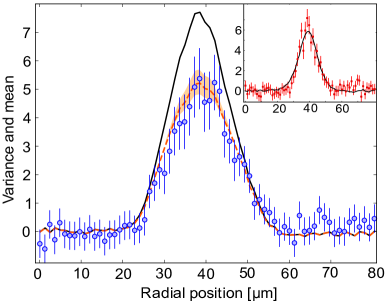
Figure 3: Spatially resolved measurement of antibunching. The black line shows the mean atom number and the blue circles the corresponding variance along the $x_{1}$-axis for a degenerate gas. The variance is rescaled using the slope fitted in Fig. 2. Error bars are estimated from the subtraction of photon shot noise, which is the dominant contribution. The dashed line shows the variance derived from theory. The shaded region indicates the uncertainty originating from uncertainties in the trap parameters. The inset shows corresponding data for a non-degenerate gas.

In contrast to previous measurements on antibunching rom_free_2006 ; jeltes_comparison_2007 , we have measured density fluctuations in a spatially resolved way. For the construction of Fig. 2, we have averaged the observed variance for regions of equal mean density, whereas Fig. 3 shows the variance (blue circles) and the mean (black line) of the atom number as a function of the radial position in the trap for a quantum degenerate gas. While the variance is proportional to the mean in the wings, at low density, we observe a reduction of the variance by about $2\,{\rm dB}$ close to the center, at higher density. The inset shows data for a non-degenerate gas; in both cases the variance has been rescaled using the slope fitted in Fig. 2. The reduction of fluctuations is a direct indication of the level of quantum degeneracy of the gas. The larger the average occupation of a single quantum state, the more the effect of the Pauli principle becomes important and fluctuations are consequently suppressed. Fig. 3 thus represents a direct measurement of the local quantum degeneracy, which is larger in the center of the cloud than in the wings.

To understand this quantitatively, we describe the atoms contained in an observation volume in terms of the grand-canonical ensemble with a local chemical potential fixed by assuming local density approximation. For a non-interacting gas, the ratio of mean atom number and its variance is determined by the fugacity $z$ of the system. This leads to the equation

$$\frac{\delta N^{2}}{\langle N\rangle}=\frac{\int\mathrm{Li}_{1/2}(-z(x_{1},x_{2}))dx_{2}}{\int\mathrm{Li}_{3/2}(-z(x_{1},x_{2}))dx_{2}},$$ (3)

where $\mathrm{Li}_{i}$ is the $i$-th polylogarithmic function, $x_{1}$ and $x_{2}$ are radial coordinates of the cloud and line-of-sight integration is performed along the $x_{2}$-axis.

The dashed line in Fig. 3 is computed using (3). For the computation we make use of the Gaussian shape of the trap, the central fugacity of $13_{-4}^{+18}$, obtained in an independent time-of-flight experiment (see below), and the experimental density profile. Our description in terms of the grand-canonical potential assuming an ideal gas reproduces the experimental data within the error bars grand-canonical .

We now focus on the interpretation of our results using the fluctuation-dissipation theorem. At thermal equilibrium, density fluctuations are universally linked to the thermodynamic properties of the gas through the fluctuation-dissipation theorem, given by

$$k_{B}T\frac{\partial\langle N\rangle}{\partial\mu}=\delta N^{2}.$$ (4)

Here $T$ is the temperature of the gas, $\mu$ the chemical potential and $k_{B}$ the Boltzmann constant. Since the local density approximation allows one to assign a local chemical potential to any position in the trap, it is possible to determine the compressibility $\frac{\partial\langle N\rangle}{\partial\mu}$ directly from the mean density profiles gemelke_in_2009 . From (4), the ratio of this quantity to the measured variance profile of the cloud provides a universal temperature measurement zhou_universal_2009 .

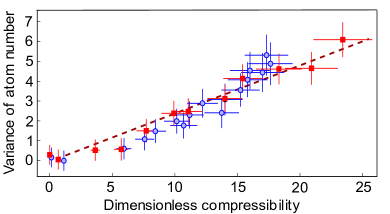
Figure 4: Fluctuation-based temperature measurement. Variance of atom number detected on an effective pixel versus dimensionless compressibility. The blue circles and red squares show the data for the quantum degenerate and the non-degenerate case, respectively. The dashed red line is fitted to the red squares, giving the temperature according to (4).

We apply this procedure to our data by computing the compressibility, $\frac{\partial\langle N\rangle}{\partial\mu}=\frac{\partial\langle N\rangle}{\partial x}\left(\frac{\partial\mu}{\partial x}\right)^{-1}$, where we take the Gaussian shape of the optical dipole trap into account. To avoid the problems of numerically differentiating experimental data, we fit the mean density profile with a linear combination of the first six even Hermite functions and use the fitted curve as a measure of the density profile in (4) hermite . Fig. 4 shows the variance of atom number plotted against the dimensionless compressibility $U_{0}\frac{\partial\langle N\rangle}{\partial\mu}$, where $U_{0}$ is the trap depth. We observe the linear relation described by (4) with a slope of $\frac{k_{B}T}{U_{0}}$ = $0.27\pm 0.04$ for both data sets, the degenerate and the non-degenerate. From the physics of evaporative cooling it is expected that both slopes are the same luiten_kinetic_1996 . Using trap depths derived from the measured laser powers, we obtain temperatures of $(145\pm 31)\,{\rm nK}$ and $(1.10\pm 0.06)\,{\rm\mu K}$ for the quantum degenerate and the non-degenerate gas, respectively.

To assess the quality of this measurement, we have also performed time-of-flight measurements with clouds prepared under the same conditions. In this method, we determine the temperatures by fitting the measured density profiles after free expansion of $1.5\,{\rm ms}$ ($1\,{\rm ms}$ for the non-degenerate gas) to the calculated shape of a non-interacting gas released from a Gaussian trap. This procedure gives us slightly higher temperatures for the degenerate and the non-degenerate clouds, which are $(205\pm 30)\,{\rm nK}$ ($T/T_{F}=0.34\pm 0.1$) and $(1.6\pm 0.2)\,{\rm\mu K}$ ($T/T_{F}=1.9\pm 0.1$), respectively. We attribute the discrepancy between the two temperature measurements to deviations of the trapping beam from a Gaussian shape and residual experimental fluctuations from shot to shot, which both affect the two methods.

In conclusion, we have measured density fluctuations in a trapped Fermi gas locally, observing antibunching in a degenerate gas. We have also determined the temperature using the fluctuation-dissipation theorem Manz_2010 . In contrast to bosons, fermions cannot exhibit first-order long range coherence due to the Pauli principle. However, when a Fermi system enters a quantum correlated phase, e.g. a superfluid phase, long range even-order correlations build up yangODLRO . The spatially resolved measurement of density fluctuations, probing second-order correlations, is thus a natural tool to study strongly correlated Fermi gases.

We acknowledge discussion with T.L. Ho, M. Greiner and D. Stadler and financial support from ERC SQMS and FP7 FET-open NameQuam.

After submission of this article, similar results were reported in sanner_suppression_2010 .

References

- (1) R. Hanbury Brown and R. Q. Twiss, Nature 178, 1046 (1956).
- (2) G. Baym, Acta Phys. Pol. B 29, 1839 (1998).
- (3) M. Yasuda and F. Shimizu, Phys. Rev. Lett. 77, 3090 (1996).
- (4) E. Altman, E. Demler, and M. D. Lukin, Phys. Rev. A 70, 013603 (2004).
- (5) A. Öttl, et al., Phys. Rev. Lett. 95, 090404 (2005).
- (6) S. Fölling, et al., Nature 434, 481 (2005).
- (7) M. Schellekens, et al., Science 310, 648 (2005).
- (8) J. Estève, et al., Phys. Rev. Lett. 96, 130403 (2006).
- (9) M. Henny, et al., Science 284, 296 (1999).
- (10) W. D. Oliver, et al., Science 284, 299 (1999).
- (11) M. Iannuzzi, et al., Phys. Rev. Lett. 96, 080402 (2006).
- (12) T. Rom, et al., Nature 444, 733 (2006).
- (13) T. Jeltes, et al., Nature 445, 402 (2007).
- (14) W. Belzig, C. Schroll, and C. Bruder, Phys. Rev. A 75, 063611 (2007).
- (15) Q. Zhou and T. Ho, arXiv:0908.3015 (2009).
- (16) N. Gemelke, et al., Nature 460, 995 (2009).
- (17) S. Jochim, et al., Science 302, 2101 (2003).
- (18) Unless otherwise stated, errors are a combination of statistical errors and uncertainties in the determination of experimental parameters.
- (19) T. L. Gustavson, et al., Phys. Rev. Lett. 88, 020401 (2001).
- (20) 4x4 software binning of camera pixels define the pixels referred to in the text. Camera pixels have an effective size (when imaged to the object plane) of 300 nm.
- (21) A. G. Basden, C. A. Haniff, and C. D. Mackay, Mon. Not. R. Astron. Soc. 345, 985 (2003).
- (22) Images deviating more than 1.5 (1.0) standard deviations, corresponding to () in the mean position (total atom number) are excluded.
- (23) A simulation accounting for the optical resolution was performed. 16x16 binning (instead of 4x4) increases the slope to 0.8 agreeing with the simulation.
- (24) J. Estève, et al., Nature 455, 1216 (2008).
- (25) The Fermi wavelength is of the order of the pixel size. However, column integration is expected to average out possible correlations.
- (26) The difference of this method with direct numerical differentiation of data (where possible) is within the error bars.
- (27) O. J. Luiten, M. W. Reynolds, and J. T. M. Walraven, Phys. Rev. A 53, 381 (1996).
- (28) For other fluctuation-based temperature measurements see S. Manz, et al., Phys. Rev. A 81, 031610 (2010) as well as R. Gati, et al., Phys. Rev. Lett. 96, 130404 (2006).
- (29) C. N. Yang, Rev. Mod. Phys. 34, 694 (1962).
- (30) The resolution of the NA=0.55 microscope objective has been artificially reduced with a diaphragm in order to increase the depth of field to the order of the cloud size.
- (31) C. Sanner, et al., 1005.1309 (2010).