Three-phase traffic theory and two-phase models with a fundamental diagram in the light of empirical stylized facts

Abstract

Despite the availability of large empirical data sets and the long history of traffic modeling, the theory of traffic congestion on freeways is still highly controversial. In this contribution, we compare Kerner’s three-phase traffic theory with the phase diagram approach for traffic models with a fundamental diagram. We discuss the inconsistent use of the term “traffic phase” and show that patterns demanded by three-phase traffic theory can be reproduced with simple two-phase models, if the model parameters are suitably specified and factors characteristic for real traffic flows are considered, such as effects of noise or heterogeneity or the actual freeway design (e.g. combinations of off- and on-ramps). Conversely, we demonstrate that models created to reproduce three-phase traffic theory create similar spatiotemporal traffic states and associated phase diagrams, no matter whether the parameters imply a fundamental diagram in equilibrium or non-unique flow-density relationships. In conclusion, there are different ways of reproducing the empirical stylized facts of spatiotemporal congestion patterns summarized in this contribution, and it appears possible to overcome the controversy by a more precise definition of the scientific terms and a more careful comparison of models and data, considering effects of the measurement process and the right level of detail in the traffic model used.

, url]http://www.mtreiber.de ,

1 Introduction

The observed complexity of congested traffic flows has puzzled traffic modelers for a long time (see Helbing (2001) for an overview). The most controversial open problems concern the issue of faster-than-vehicle characteristic propagation speeds (Daganzo, 1995; Aw and Rascle, 2000) and the question whether traffic models with or without a fundamental diagram (i.e. with or without a unique equilibrium flow-density or speed-distance relationship) would describe empirical observations best. While the first issue has been intensively debated recently (see Helbing and Johansson (2009), and references therein), this paper addresses the second issue.

The most prominent approach regarding models without a fundamental diagram is the three-phase traffic theory by (Kerner, 2004). The three phases of this theory are “free traffic”, “wide moving jams”, and “synchronized flow”. While a characteristic feature of “synchronized flow” is the wide scattering of flow-density data (Kerner and Rehborn, 1996b), many microscopic and macroscopic traffic models neglect noise effects and the heterogeneity of driver-vehicle units for the sake of simplicity, and they possess a unique flow-density or speed-distance relationship under stationary and spatially homogeneous equilibrium conditions. Therefore, Appendix A discusses some issues concerning the wide scattering of congested traffic flows and how it can be treated within the framework of such models.

For models with a fundamental diagram, a phase diagram approach has been developed (Helbing et al., 1999) to represent the conditions under which certain traffic states can exist. A favourable property of this approach is the possibility to semi-quantitatively derive the conditions for the occurence of the different traffic states from the instability properties of the model under consideration and the outflow from congested traffic (Helbing et al., 2009). The phase diagram approach for models with a fundamental diagram has recently been backed up by empirical studies (Schönhof and Helbing, 2009). Nevertheless, the approach has been criticized (Kerner, 2002, 2008), which applies to the alternative three-phase traffic theory as well (Schönhof and Helbing, 2007, 2009). While both theories claim to be able to explain the empirical data, particularly the different traffic states and the transitions between them, the main dispute concerns the following points:

• Both approaches use an inconsistent terminology regarding the definition of traffic phases and the naming of the traffic states.

• Both modeling approaches make simplifications, but are confronted with empirical details they were not intended to reproduce (e.g. effects of details of the freeway design, or the heterogeneity of driver-vehicle units).

• three-phase traffic theory is criticized for being complex, inaccurate, and inconsistent, and related models are criticized to contain too many parameters to be meaningful (Helbing and Treiber, 2002; Schönhof and Helbing, 2007).

• It is claimed that the phase diagram of models with a fundamental diagram would not represent the empirical observed traffic states and transitions well (Kerner, 2004). In particular, the “general pattern” (GP) and the “widening synchronized pattern” (WSP) would be missing. Moreover, wide moving jams should always be part of a “general pattern”, and homogeneous traffic flows should not occur for extreme, but rather for small bottleneck strengths.

In the following chapters, we will try to overcome these problems. In Sec. 2 we will summarize the stylized empirical facts that are observed on freeways in many different countries and have to be explained by realistic traffic models. Afterwards, we will discuss and clarify the concept of traffic phases in Sec. 3. In Sec. 4, we show that the traffic patterns of three-phase traffic theory can be simulated by a variety of microscopic and macroscopic traffic models with a fundamental diagram, if the model parameters are suitably chosen. For these model parameters, the resulting traffic patterns look surprisingly similar to simulation results for models representing three-phase traffic theory, which have a much higher degree of complexity. Depending on the interest of the reader, he/she may jump directly to the section of interest. Finally, in Sec. 5, we will summarize and discuss the alternative explanation mechanisms, pointing out possible ways of resolving the controversy.

2 Overview of empirical observations

In this section, we will pursue a data-oriented approach. Whenever possible, we describe the observed data without using technical terms used within the framework of three-phase traffic theory or models with a fundamental diagram. In order to show that the following observations are generally valid, we present data from several freeways in Germany, not only from the German freeway A5, which has been extensively studied before (Kerner, 1998; Kerner and Rehborn, 1996a; Schönhof and Helbing, 2007, 2009; Bertini et al., 2004; Lindgren et al., 2006). Our data from a variety of other countries confirm these observations as well (Zielke et al., 2008).

2.1 Data issues

In order to eliminate confusion arising from different interpretations of the data and to facilitate a direct comparison between computer simulations and observations, one has to simulate the method of data acquisition and the subsequent processing or interpretation steps as well. We will restrict ourselves here to the consideration to aggregated stationary detector data which currently is the main data source of freeway traffic studies. When comparing empirical and simulation data, we will focus on the velocity $V$ (and not the density), since it can be measured directly. In addition to the aggregation over one-minute time intervals, we will also aggregate over the freeway lanes. This is justified due to the typical synchronization of velocities among freeway lanes in all types of congested traffic (Helbing and Treiber, 2002).

To simulate the measurement and interpretation process, we use “virtual detectors” recording the passage time and velocity of each vehicle. For each aggregation time interval (typically 60 s), we determine the traffic flow $Q$ as the vehicle count divided by the aggregation time, and the velocity $V$ as the arithmetic mean value of the individual vehicles passing in this time period. Notice that the arithmetic mean value leads to a systematic overestimation of velocities in congested situations and that there exist better averaging methods such as the harmonic mean (Treiber et al., 2000a). Nevertheless, we will use the above procedure because this is the way in which empirical data are typically evaluated by detectors.

Since freeway detectors are positioned only at a number of discrete locations, interpolation techniques have to be applied to reconstruct the observed spatiotemporal dynamics at any point in a given spatiotemporal region. If the detector locations are not further apart than about 1 km, it is sufficient to apply a linear smoothing/interpolating filter, or even to plot the time series of the single detectors in a suitable way (see, e.g. Fig. 1 in Schönhof and Helbing (2007)). This condition, however, severely restricts the selection of suitable freeway sections, which is one of the reasons why empirical traffic studies in Germany have been concentrated on a 30 km long section of the Autobahn A5 near Frankfurt. For most other freeway sections showing recurrent congestion patterns, two neighboring detectors are 1-3 km apart, which is of the same order of magnitude as typical wavelengths of non-homogeneous congestion patterns and therefore leads to ambiguities as demonstrated by Treiber and Helbing (2002). Furthermore, the heterogeneity of traffic flows and measurement noise lead to fluctuations obscuring the underlying patterns.

Both problems can be overcome by post-processing the aggregated detector data (Cassidy and Windower, 1995; Coifman, 2002; Bertini et al., 2004; Muñoz and Daganzo, 2002; Belomestny et al., 2003; Treiber and Helbing, 2002). Furthermore, Kerner et al. (2001) have proposed a method called “ASDA/FOTO” for short-term traffic prediction. Most of these methods, however, cannot be applied for the present investigation since they do not provide continuous velocity estimates for all points $(x,t)$ of a certain spatiotemporal region, or because they are explicitly based on models. (The method ASDA/FOTO, for example, is based on three-phase traffic theory.) We will therefore use the adaptive smoothing method (Treiber and Helbing, 2002), which has recently been validated with empirical data of very high spatial resolution (Treiber et al., 2010). In order to be consistent, we will apply this method to both, the real data and the virtual detector data of our computer simulations.

2.2 Spatiotemporal data

In this section, we will summarize the stylized facts of the spatiotemporal evolution of congested traffic patterns, i.e., typical empirical findings that are persistently observed on various freeways all over the world. In order to provide a comprehensive list as a testbed for traffic models and theories, we will summarize below all relevant findings, including already published ones:

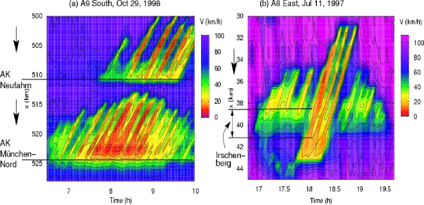
Figure 1: Spatiotemporal dynamics of the average velocity on two different freeways. (a) German freeway A9 in direction South, located in the area North of Munich. Horizontal lines indicate two intersections (labelled “AK”), which cause bottlenecks, since they consume some of the freeway capacity. The traffic direction is shown by arrows. (b) German freeway A8 in direction East, located about 40 km East of Munich. Here, the bottlenecks are caused by uphill and downhill gradients around “Irschenberg” and by an accident at $x=43.5\,\mathrm{km}$ in the time period between 17:40 h and 18:20 h.

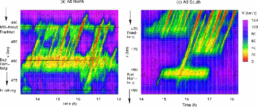
Figure 2: Spatiotemporal velocity profiles for the German freeway A5 North near Frankfurt/Main (both directions). Arrows indicate the direction of travel.

1. Congestion patterns on real (non-circular) freeways are typically caused by bottlenecks in combination with a perturbation in the traffic flow. An extensive study of the breakdown phenomena on the German freeways A5-North and A5-South by Schönhof and Helbing (2007), analyzing about 400 congestion patterns, did not find examples where there was an apparent lack of a bottleneck. This is in agreement with former investigations of the Dutch freeway A9, the German freeway A8-East and West, and the German freeway A9-South (Treiber et al., 2000a). Nevertheless, it may appear to drivers entering a traffic jams on a homogeneous freeway section that they are experiencing a ”phantom traffic jam”, i.e. a traffic jam without any apparent reason. In these cases, however, the triggering bottleneck, which is actually the reason for the traffic jam, is located downstream, potentially in a large distance from the driver location (see Fig. 13 of Schönhof and Helbing (2007) or in Fig. 1(a) of Helbing et al. (2009)).

2. The bottleneck may be caused by various reasons such as isolated on-ramps or off-ramps, combinations thereof such as junctions or intersections (Fig. 1(a) and 2), local narrowings or reductions of the number of lanes, accidents, or gradients. As an example, Fig. 1(b) shows a composite congestion pattern on the German freeway A8-East caused by uphill and downhill gradients (“Irschenberg”) in the region $38\,\mathrm{km}\leq x\leq 41\,\mathrm{km}$, and an additional obstruction by an accident at $x=43.5\,\mathrm{km}$ in the time period between 17:40 h and 18:15 h.

3. The congestion pattern is either localized with a constant width of the order of 1 km, or it is spatially extended with a time-dependent extension. Localized congestion patterns either remain stationary at the bottleneck, or they move upstream at a characteristic speed $c_{\rm cong}$. Typical values of $c_{\rm cong}$ are between $-20\,\mathrm{km/h}$ and $-15\,\mathrm{km/h}$, depending on the country and traffic composition (Zielke et al., 2008), but not on the type of congestion. About 200 out of 400 breakdowns observed by Schönhof and Helbing (2007) correspond to extended patterns.

4. The downstream front of congested traffic is either fixed at the bottleneck, or it moves upstream with the characteristic speed $c_{\rm cong}$ (Helbing et al., 2009). Both, fixed and moving downstream fronts can occur within one and the same congestion pattern. This can be seen in Fig. 1(a), where the stationary downstream congestion front at $x=476\,\mathrm{km}$ (the location of the temporary bottleneck caused by an incident) starts moving upstream at 17:30 h. Such a “detachment” of the downstream congestion front occurs, for example, when an accident site has been cleared, and it is one of two ways in which the dissolution of traffic congestion starts (see next item for the second one).

5. The upstream front of spatially extended congestion patterns has no characteristic speed. Depending on the traffic demand and the bottleneck capacity, it can propagate upstream (if the demand exceeds the capacity) or downstream (if the demand is below capacity) (Helbing et al., 2009). This can be seen in all extended congestion patterns of Fig. 1 (see also Schönhof and Helbing (2009); Kerner (2004)). The downstream movement of the congestion front towards the bottleneck is the second and most frequent way in which congestion patterns may dissolve.

6. Most extended traffic patterns show some “internal structure” propagating upstream approximately at the same characteristic speed $c_{\rm cong}$. Consequently, all spatiotemporal structures in Figs. 1 and 2 (sometimes termed “oscillations”, “stop-and-go traffic”, or “small jams”), move in parallel (Smilowitz et al., 1999; Mauch and Cassidy, 2002; Zielke et al., 2008).

7. The periods and wavelengths of internal structures in congested traffic states tend to decrease as the severity of congestion increases. This applies in particular to measurements of the average velocity. (See, for example, Fig. 1(a), where the greater of two bottlenecks, located at the Intersection München-Nord, produces oscillations of a higher frequency. Typical periods of the internal quasi-periodic oscillations vary between about 4 min and 60 min, corresponding to wavelengths between 1 km and 15 km (Helbing and Treiber, 2002).

8. For bottlenecks of moderate strength, the amplitude of the internal structures tends to increase while propagating upstream. This can be seen in all empirical traffic states shown in this contribution, and also in Schönhof and Helbing (2009); Helbing et al. (2009). It can also be seen in the corresponding velocity time series, such as the ones in Fig. 12 of Treiber et al. (2000a), in Zielke et al. (2008), or in all relevant time series shown in Chapters 9-13 of Kerner (2004). The oscillations may already be visible at the downstream boundary (Fig. 1(b)), or emerge further upstream (Figs. 1(a), 2(a)). During their growth, neighboring perturbations may merge (Fig. 1 in Schönhof and Helbing (2009)), or propagate unaffected (Fig. 1). At the upstream end of the congested area, the oscillations may eventually become isolated “wide jams” (Fig. 2) or remain part of a compact congestion pattern (Fig. 1).

9. Light or very strong bottlenecks may cause extended traffic patterns, which appear homogeneous (uniform in space), see, for example, Figs. 1(d) and 1(f) of  Helbing et al. (2009). Note however that, for strong bottlenecks (typically caused by accidents), the empirical evidence has been controversially debated, in particular as the oscillation periods at high densities reach the same order of magnitude as the smoothing time window that has typically been used in previous studies (cf. point 7 above). This makes oscillations hardly distinguishable from noise. See Appendix B for a further discussion of this issue.

Note that the above stylized facts have not only be observed in Germany, but also in other countries, e.g. the USA, Great Britain, and the Netherlands (Zielke et al., 2008; Helbing et al., 2009; Wilson, 2008a; Treiber et al., 2010). Furthermore, we find that many congestion patterns are composed of several of the elementary patterns listed above (Schönhof and Helbing, 2007). For example, the congestion pattern observed in Fig. 2(b) can be decomposed into moving and stationary localized patterns as well as extended patterns.

The source of probably most controversies in traffic theory is an observed spatiotemporal structure called the “pinch effect” or “general pattern” (Kerner and Rehborn, 1996b), see Kerner (2004) for details and Fig. 1 of Schönhof and Helbing (2009) for a typical example of the spatiotemporal evolution. From the perspective of the above list, this pattern relates to stylized facts 6 and 8, i.e., it has the following features: (i) relatively stationary congested traffic (pinch region) near the downstream front, (ii) small perturbations that grow to oscillatory structures as they travel further upstream, (iii) some of these structures grow to form “wide jams”, thereby suppressing other small jams, which either merge or dissolve. The question is whether this congestion pattern is composed of several elementary congestion patterns or a separate, elementary pattern, which is sometimes called “general pattern” (Kerner, 2004). This will be addressed in Sec. 4.3.

3 The meaning of traffic phases

The concept of “phases” has originally been used in areas such as thermodynamics, physics, and chemistry. In these systems, “phases” mean different aggregate states (such as solid, fluid, or gaseous; or different material compositions in metallurgy; or different collective states in solid state physics). When certain “control parameters” such as the pressure or temperature in the system are changed, the aggregate state may change as well, i.e. a qualitatively different macroscopic organization of the system may result. If the transition is abrupt, one speaks of first-order (or “hysteretic”, history-dependent) phase transitions. Otherwise, if the transition is continuous, one speaks of second-order phase transitions.

In an abstract space, whose axes are defined by the control parameters, it is useful to mark parameter combinations, for which a phase transition occurs, by lines or “critical points”. Such illustrations are called phase diagrams, as they specify the conditions, under which certain phases occur.

Most of the time, the terms “phase” and “phase diagram” are applied to large (quasi-infinite), spatially closed, and homogeneous systems in thermodynamic equilibrium, where the phase can be determined in any point of the system. When transferring these concepts to traffic flows, researchers have distinguished between one-phase, two-phase, and three-phase models. The number of phases is basically related to the (in) stability properties of the traffic flows (i.e. the number of states that the instability diagram distinguishes). The equilibrium state of one-phase models is a spatially homogeneous traffic state (assuming a long circular road without any bottleneck). An example would be the Burgers equation (Whitham, 1974), i.e. a Lighthill–Whitham–Richard model (Lighthill and Whitham, 1955; Richards, 1956) with diffusion term. Two-phase models would additionally produce oscillatory traffic states such as wide moving jams or stop-and-go waves, i.e. they require some instability mechanism (Wagner and Nagel, 2008).Three-phase models introduce another traffic state, so-called “synchronized flow”, which is characterized by a self-generated scattering of the traffic variables. It is not clear, however, whether this state exists in reality in the absence of spatial inhomogeneities (freeway bottlenecks).

Note, however, that the concept of phase transitions has also been transferred to non-equilibrium systems, i.e. driven, open systems with a permanent inflow or outflow of energy, inhomogeneities, etc. This use is common in systems theory. For example, one has introduced the concept of boundary-induced phase transitions (Krug, 1991; Popkov et al., 2001; Appert and Santen, 2001). From this perspective, the Burgers equation can show a boundary-induced phase transition from a free-flow state with forwardly propagating congestion fronts to a congested state with upstream moving perturbations of the traffic flow. This implies that the Burgers equation (with one equilibrium phase) has two non-equilibrium phases. Analogously, two-phase models (in the previously discussed, thermodynamic sense) can have more than two non-equilibrium phases. However, to avoid confusion, one often uses the terms “(spatiotemporal) traffic patterns” or “(elementary) traffic states” rather than “non-equilibrium phases”. For example, the gas-kinetic-based traffic model (GKT model) or the intelligent driver model (IDM), which are two-phase models according to the above classification, may display several congested traffic states besides free traffic flow (Treiber et al., 2000a). The phase diagram approach to traffic modeling proposed by Helbing et al. (1999) was originally presented for an open traffic system with an on-ramp. It shows the qualitatively different, spatiotemporal traffic patterns as a function of the freeway flow and the bottleneck strength.

Note, however, that the resulting traffic state may depend on the history (e.g. the size of perturbations in the traffic flow), if traffic flows have the property of metastability.

The concept of the phase diagram has been taken up by many authors and applied to the spatiotemporal traffic patterns (non-equilibrium phases) produced in many models (Lee et al., 1998, 1999; Kerner, 2004; Siebel and Mauser, 2006). Besides on-ramp scenarios, one may study scenarios with flow-conserving bottlenecks (such as lane closures or gradients) or with combinations of several bottlenecks. It appears, however, that the traffic patterns for freeway designs with several bottlenecks can be understood, based on the combination of elementary traffic patterns appearing in a system with a single bottleneck and interaction effects between these patterns (Schönhof and Helbing, 2007; Helbing et al., 2009)

The resulting traffic patterns as a function of the flow conditions and bottleneck strengths (freeway design), and therefore the appearance of the phase diagram, depend on the traffic model and the parameters chosen. Therefore, the phase diagram approach can be used to classify the large number of traffic models into a few classes. Models with qualitatively similar phase diagrams would be considered equivalent, while models producing different kinds of traffic states would belong to different classes. The grand challenge of traffic theory is therefore to find a model and/or model parameters, for which the congestion patterns match the stylized facts (see Sec. 2.2) and for which the phase diagram agrees with the empirical one (Schönhof and Helbing, 2007; Helbing et al., 2009). This issue will be addressed in Sec. 4

For the understanding of traffic dynamics one may ask which of the two competing phase definitions (the thermodynamic or the non-equilibrium one) would be more relevant for observable phenomena. Considering the stylized facts (see Sec. 2), it is obvious that boundary conditions and inhomogeneities play an important role for the resulting traffic patterns. This clearly favours the dynamic-phase concept over the definition of thermodynamic equilibrium phases: Traffic patterns are easily observable and also relevant for applications. (For calculating traveling times, one needs the spatiotemporal dynamics of the traffic pattern, and not the thermodynamic traffic phase.) Moreover, thermodynamic phases are not observable in the strict sense, because real traffic systems are not quasi-infinite, homogeneous, closed systems. Consequently, when assessing the quality of a given model, it is of little relevance whether it has two or three physical phases, as long as it correctly predicts the observed spatiotemporal patterns, including the correct conditions for their occurrence. Nevertheless, the thermodynamic phase concept (the instability diagram) is relevant for explaining the mechanisms leading to the different patterns. In fact, for models with a fundamental diagram, it is possible to derive the phase diagram of traffic states from the instability diagram, if bottleneck effects and the outflow from congested traffic are additionally considered (Helbing et al., 1999).

4 Simulating the spatiotemporal traffic dynamics

In the following, we will show for specific traffic models that not only three-phase traffic theory, but also the conceptionally simpler two-phase models (as introduced in Sec. 3) can display all stylized facts mentioned in Sec. 2, if the model parameters are suitably chosen. This is also true for patterns that were attributed exclusively to three-phase traffic theory such as the pinch effect or the widening synchronized pattern (WSP).

Considering the dynamic-phase definition of Sec. 3, the simplest system that allows to reproduce realistic congestion patterns is an open system with a bottleneck. When simulating an on-ramp bottleneck, the possible flow conditions can be characterized by the upstream freeway flow (“main inflow”) and the ramp flow, considering the number of lanes (Helbing et al., 1999). The downstream traffic flow under free and congested conditions can be determined from these quantities. When simulating a flow-conserving (ramp-less) bottleneck, the ramp flow is replaced by the bottleneck strength quantifying the degree of local capacity reduction (Treiber et al., 2000b).

Since many models show hysteresis effects, i.e. discontinuous, history-dependent transitions, the time-dependent traffic conditions before the onset of congestion are relevant as well. In the simplest case, the response of the system is tested (i) for minimum perturbations, e.g. slowly increasing inflows and ramp flows, and (ii) for a large perturbation. The second case is usually studied by generating a wide moving jam, which can be done by temporarily blocking the outflow. Additionally, the model parameters characterizing the bottleneck situation have to be systematically varied and scanned through. This is, of course, a time-consuming task since producing a single point in this multi-dimensional space requires a complete simulation run (or even to average over several simulation runs).

4.1 Two-phase models

Wagner and Nagel (2008) classify models with a fundamental diagram that show dynamic traffic instabilities in a certain density range, as two-phase models. Alternatively, these models are referred to as “models within the fundamental diagram approach”. Note, however, that certain models with a unique fundamental diagram are one-phase models (such as the Burgers equation). Moreover, some models such as the KK model can show one-phase, two-phase or three-phase behavior, depending on the choice of model parameters (see Sec. 4.2).

A microscopic two-phase model necessarily has a dynamic acceleration equation or contains time delays such as a reaction time. For macroscopic models, a necessary (but not sufficient) condition for two phases is that the model contains a dynamical equation for the macroscopic velocity.

4.1.1 Traffic patterns for a macroscopic traffic model

We start with results for the gas-kinetic-based traffic model (Helbing, 1996; Treiber et al., 1999). Like other macroscopic traffic models, the GKT model describes the dynamics of aggregate quantities, but besides the vehicle density $\rho(x,t)$ and average velocity $V(x,t)$, it also considers the velocity variance $\theta(x,t)=A(\rho(x,t))V(x,t)^{2}$ as a function of velocity and density.

The GKT model has five parameters $v_{0}$, $T$, $\tau$, $\gamma$, and $\rho_{\rm max}$ characterizing the driver-vehicle units, see Table 1. In contrast to other popular second-order models (Payne, 1971; Kerner and Konhäuser, 1993; Lee et al., 1999; Hoogendoorn and Bovy, 2000), the GKT model distinguishes between the desired time gap $T$ when following other vehicles, and the much larger acceleration time $\tau$ to reach a certain desired velocity. Furthermore, the drivers of the GKT model “look ahead” by a certain multiple $\gamma$ of the distance to the next vehicle. The GKT model also contains a variance function $A(\rho)$ reflecting statistical properties of the traffic data. Its form can be empirically determined (see Table 1). For the GKT model equations, we refer to Treiber et al. (1999).

Table 1: The two parameter sets for the GKT model (Treiber et al., 1999) used in this paper. The four last parameters specify the velocity variance prefactor $A(\rho)=A_{0}+(A_{\rm max}-A_{0})/2\{\tanh[(\rho-\rho_{\rm c})/\Delta\rho]+1\}$

Model parameter	Value set 1	Value set 2
Desired velocity $v_{0}$	120 km/h	120 km/h
Desired time gap $T$	1.35 s	1.8 s
Acceleration time $\tau$	20 s	35 s
Anticipation factor $\gamma$	1.1	1.0
Maximum density $\rho_{\rm max}$	140/km	140/km
Variance prefactor $A_{0}$ for free traffic	0.008	0.01
Variance prefactor $A_{\rm max}$ for congested traffic	0.038	0.03
Transition density free-congested $\rho_{c}$	$0.27~{}\rho_{\rm max}$	$0.4~{}\rho_{\rm max}$
Transition width $\Delta\rho$	$0.07~{}\rho_{\rm max}$	$0.05~{}\rho_{\rm max}$

We have simulated an open system with an on-ramp as a function of the main flow and the ramp flow, using the two parameter sets listed in Table 1. In contrast to the simulations in Helbing et al. (1999), we added variations of the on-ramp flow with an amplitude of 20 vehicles/h and a mean value of zero to compensate for the overly smooth merging dynamics in macroscopic models, when mergings are just modeled by constant (or slowly varying) source terms in the continuity equation. For parameter set 1, we obtain the results of Fig. 3, i.e., the phase diagram found by Helbing et al. (1999) and by Lee et al. (1998). It contains five congested traffic patterns, namely pinned localized clusters (PLC), moving localized clusters (MLC), triggered stop-and-go waves (TSG), oscillating congested traffic (OCT), and homogeneous congested traffic (HCT). The OCT and TSG patterns look somewhat similar, and there is no discontinuous transition between these patterns. This has been indicated by a dashed instead of a solid line in the phase diagram. Furthermore, notice that the two localized patterns MLC and PLC are only obtained, when sufficiently strong temporary perturbations occur in addition to the stationary on-ramp bottleneck. Such perturbations may, for example, result from a temporary peak in the ramp flow or in the main inflow (which may be caused by forming vehicle platoons, when slower trucks overtake each other, see Schönhof and Helbing (2007)). Furthermore, the perturbation may be an upstream moving traffic jam entering a bottleneck area (see Fig. 2(b) and Helbing et al. (1999)). This case has been assumed here.

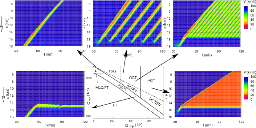
Figure 3: Congested traffic patterns as a function of the dynamic phase space spanned by the main inflow and the ramp inflow for the GKT model with parameter set 1 in Table 1. The dotted line indicates the maximum traffic demand for which free flow can be sustained. Below this line, congestion patterns can only be triggered by perturbations. For this purpose, a moving jam has been generated at the downstream boundary in the two plots on the left-hand side. The abbreviations denote free traffic (FT), pinned localized cluster (PLC), moving localized cluster (MLC), homogeneous congested traffic (HCT), oscillatory congested traffic (OCT), and triggered stop-and-go (TSG) pattern.

When simulating the same system, but this time using parameter set 2 of Table 1, we obtain the PLC, MLC, OCT and HCT states as in the first simulation, see Fig. 4 (the MLC pattern is not shown). However, instead of the TSG state, we find two new patterns. For very light bottlenecks (small ramp flows), we observe a light form of homogeneous congested traffic that has the properties of the widening synchronized pattern (WSP) proposed by Kerner (2004). Remarkably, this state is stable or metastable, otherwise moving jams should emerge from it in the presence of small-amplitude variations of the ramp flow. Although the WSP-properties of being extended and homogeneous in space are the same as for the HCT state, WSP occurs for light bottlenecks, while HCT requires strong bottlenecks. Moreover, the two patterns are separated in the phase diagram by oscillatory states that occur for moderate bottleneck strengths.

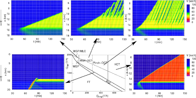
Figure 4: Dynamic phase diagram of congested traffic patterns for the GKT model as in Fig. 3, but this time using parameter set 2 from Table 1. While the TSG pattern is missing, the two additional patterns “pinch region” and WSP (widening synchronized pattern) are produced (see the main text for details).

The second new traffic pattern is a congested state which consists of a stationary downstream front at the on-ramp bottleneck, homogeneous, light congested traffic near the ramp, and velocity oscillations (“small jams” or OCT) further upstream. These are the signatures of the pinch effect. Similarly to the transition TSG$\leftrightarrow$OCT in the dynamic phase diagram of Fig. 3, there is no sharp transition between light congested traffic and OCT.

The corresponding stability diagrams shown in Fig. 5 for the two parameter sets are consistent with these findings: In contrast to parameter set 1, parameter set 2 leads to a small density range of metastable (rather than unstable) congested traffic near the maximum flow, which is necessary for the occurence of the WSP. Furthermore, parameter set 2 leads to a wide density range of convectively unstable traffic, which favours the pinch effect as will be discussed in Sec. 4.3.2.

Finally, we note that the transition from free traffic to extended congested traffic is of first order. The associated hysteresis (capacity drop) is reflected in the phase diagram of Fig. 4 by the vertical distance between the dotted line and the line separating the PLC pattern from spatially extended traffic patterns, and also by the large metastable density regime in the stability diagram (see Fig. 5). Note, that the optimal velocity model, in contrast, behaves nonhysteretic (Kerner and Klenov, 2006, Sec. 6.2), which is not true for the microscopic models discussed in the next subsection.

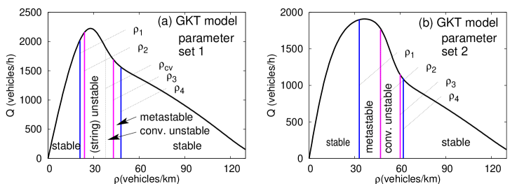
Figure 5: Fundamental diagrams and stability regimes of the GKT model for the two parameter sets in Table 1. The so-called critical densities $\rho_{1}$, $\rho_{2}$, $\rho_{3}$, and $\rho_{4}$ correspond to the densities at which the transitions stable$\leftrightarrow$metastable$\leftrightarrow$unstable$\leftrightarrow$metastable$\leftrightarrow$stable occur. For $\rho>\rho_{\rm cv}$, the instabilities are of a convective type. For the existence of a widening synchronized pattern (WSP), the critical density $\rho_{2}$ must be on the “congested” side of the fundamental diagram.

4.1.2 Traffic patterns in microscopic traffic models

In order to investigate the generality of the above results, we have simulated the same traffic system also with the intelligent driver model (IDM) as one representative of two-phase microscopic traffic models with continuous dynamics (Treiber et al., 2000a).

The IDM specifies the acceleration $dv_{\alpha}/dt$ of vehicle $\alpha$ following a leader $\alpha-1$ (with the bumper-to-bumper distance $s_{\alpha}$ and the relative velocity $\Delta v_{\alpha}=v_{\alpha}-v_{\alpha-1}$) as a continuous deterministic function with five model parameters. The desired velocity $v_{0}$ and the time gap $T$ in equilibrium have the same meaning as in the GKT model. The actual acceleration is limited by the maximum acceleration $a$. The “intelligent” braking strategy generally limits the decelerations, to the comfortable value $b$, but it allows for higher decelerations if this is necessary to prevent critical situations or accidents. Finally, the gap to the leading vehicle in standing traffic is represented by $s_{0}$. Notice that the sum of $s_{0}$ and the (dynamically irrelevant) vehicle length $l_{0}$ is equivalent to the inverse of the GKT parameter $\rho_{\rm max}$.

It has been shown that the IDM is able to produce the five traffic patterns PLC, MLC, TSG, OCT, and HCT found in the GKT model with parameter set 1 (Treiber et al., 2000a). Here, we want to investigate whether the IDM can also reproduce the “new” patterns shown in Fig. 4, i.e., the WSP and the pinch effect. For this purpose, we slightly modify the simulation model as compared to the assumptions made in previous publications:

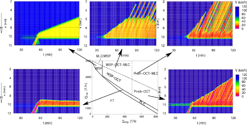
Figure 6: Dynamic phase diagram of on-ramp-induced congested traffic patterns for the Intelligent Driver Model with the parameters given in Sec. 4.1.2. As in the previous diagrams, the dashed line indicates the maximum traffic volume for which free flow can be sustained. In order to trigger the congestion patterns at the bottleneck, a moving jam is introduced at the downstream boundary for the three simulations corresponding to points below the dashed line (metastable regimes).

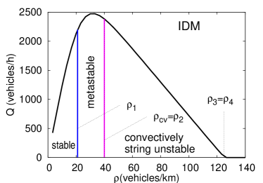
Figure 7: Fundamental diagram and stability regions of the IDM for the parameters $v_{0}=120\,\mathrm{km/h}$, $T=1\,\mathrm{s}$, $s_{0}=2\,\mathrm{m}$, $a=1.2\,\mathrm{m/s^{2}}$, and $b=1.3\,\mathrm{m/s^{2}}$ used in this paper. In contrast to the original specifications by Treiber et al. (2000a), traffic flow at capacity is metastable rather than linearly unstable here, and the linear string instability for higher densities is always of the convective type. See Fig. 5 for the definition of the critical densities $\rho_{i}$ and $\rho_{\rm cv}$.

• Instead of a “flow-conserving bottleneck” we simulate an on-ramp. Since the focus is not on realistic lane-changing and merging models we simulate here a main road consisting only of one lane and keep the merging rule simple: As soon as an on-ramp vehicle reaches the merging zone of 600 m length, it is centrally inserted into the largest gap within the on-ramp zone with a velocity of 60% of the actual velocity of the leading vehicle on the destination lane.

• The IDM parameters have been changed such that traffic flow at maximum capacity is metastable rather than linearly unstable. This can be reached by increasing the maximum acceleration $a$. Specifically, we assume $v_{0}=120\,\mathrm{km/h}$, $T=1\,\mathrm{s}$, $s_{0}=2\,\mathrm{m}$, $a=1.2\,\mathrm{m/s^{2}}$, and $b=1.3\,\mathrm{m/s^{2}}$. Furthermore, the vehicle length $l_{0}$ is set to 6 m. Note that there is actually empirical evidence that flows are metastable at densities corresponding to capacity  (Helbing and Tilch, 2009; Helbing et al., 2009): A growing vehicle platoon behind overtaking trucks is stable, as long as there are no significant perturbations in the traffic flow. However, weaving flows close to ramps can produce perturbations that are large enough to cause a traffic breakdown, when the platoon reaches the neighborhood of the ramp.

Figure 6 shows that, with one exception, the congestion patterns obtained for the IDM model with (meta-)stable maximum flow are qualitatively the same as for the GKT model with parameter set 2 (see Fig. 4). As for the GKT model, all transitions from free to congested states are hysteretic, i.e., the corresponding regions in the phase diagram extend below the dashed line, where free traffic can be sustained as well. In this case, free traffic downstream of the on-ramp is at or below (static) capacity, and therefore metastable (cf. Fig. 7). Consequently, a sufficiently strong perturbation is necessary to trigger the WSP, PLC, or OCT states. Specifically, for the WSP, PLC, and Pinch-OCT simulations of Fig. 6, the perturbations associated with the mergings at the ramp are not strong enough and an external perturbation (a moving jam) is necessary to trigger the congested states.

In contrast to the GKT simulations, however, the HCT state is obviously missing. Even for the maximum ramp flows, where merging is possible for all vehicles (about 1000 vehicles/h), the congested state behind the on-ramp remains oscillatory. This is consistent with the corresponding stability diagram in Fig. 7, which shows no restabilization of traffic flows at high densities, i.e. the critical densities $\rho_{3}$ and $\rho_{4}$ do not exist. This finding, however, depends on the parameters. It can be analytically shown (Helbing et al., 2009) that a HCT state exists, if

$$s_{0}<aT^{2}.$$ (1)

This means, when varying the minimum distance $s_{0}$ and leaving all other IDM parameters constant (at the values given above), a phase diagram of the type shown in Fig. 4 (containing oscillatory and homogeneous congested traffic patterns) exists for $s_{0}\leq 1.2\,\mathrm{m}$, while a phase diagram as in Fig. 6 (without restabilization at high densities) results for $s_{0}>1.2\,\mathrm{m}$. Moreover, when varying the acceleration parameter $a$ and leaving all other IDM parameters at the values given above, the IDM phase diagram is of the type displayed in Fig. 6, if $0.93\,\mathrm{m/s^{2}}\leq a<1.3\,\mathrm{m/s^{2}}$, but of the type shown in the original phase diagram by Treiber et al. (2000a) (without a WSP state), if $a<0.93\,\mathrm{m/s^{2}}$, and of the type belonging to a single-phase model (with homogeneous traffic states only), if $a>1.3\,\mathrm{m/s^{2}}$.

We obtain the surprising result that, in contrast to the IDM parameters chosen by Treiber et al. (2000a), homogeneous congested traffic of the WSP type can be observed even for very small bottleneck strengths, while the pinch effect is observed for intermediate bottleneck strengths and a sufficiently high inflow on the freeway into the bottleneck area. Furthermore, no restabilization takes place for strong bottlenecks, in agreement with what is demanded by Kerner (2008). Notice that the empirically observed oscillations are not perfectly periodic as in Fig. 6, but quasi-periodic with a continuum of elementary frequencies concentrated around a typical frequency (corresponding to a period of about 3.5 min in the latter reference). In computer simulations, such a quasi-periodicity is obtained for heterogeneous driver-vehicle units with varying time gaps.

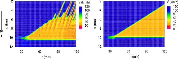
Figure 8: Congestion patterns caused (a) by an on-ramp bottleneck, and (b) by a comparable flow-conserving bottleneck (resulting in the same average traffic flow in the congested region). The simulations were performed with the IDM, using the same parameters as specified in the main text before.

Clearly, the merging rule generates considerable noise at the on-ramp. It is therefore instructive to compare the on-ramp scenario with a scenario assuming a flow-conserving bottleneck, but the same model and the same parameters. Therefore, it is instructive to simulate a flow-conserving bottleneck rather than an on-ramp bottleneck. Formally, we have implemented the flow-conserving bottleneck by gradually increasing the time gap $T$ from 1.0 s to a higher value $T_{\rm bottl}$ within a 600 m long region as in Treiber et al. (2000a), keeping $T=T_{\rm bottl}$ further downstream. The value of $T_{\rm bottl}$ determines the effectively resulting bottleneck strength. We measure the bottleneck strength as the difference of the outflow from wide moving jams sufficiently away from the bottleneck and the average flow in the congested area upstream of it (Treiber et al., 2000b).

Performing exactly the same simulations as in Fig. 6, but replacing the on-ramp bottleneck by a flow-conserving bottleneck, we find essentially no difference for most combinations of the main inflow and the bottleneck strength. However, a considerable fraction of the parameter space leading to a pinch effect in the on-ramp system results in a WSP state in the case of the flow-conserving bottleneck. Figure 8 shows the direct comparison for a main inflow of $Q_{\rm in}=2000\,\mathrm{vehicles/h}$, and a ramp flow of $Q_{\rm rmp}=250\,\mathrm{vehicles/h}$, corresponding to $T_{\rm bottl}=1.37\,\mathrm{s}$ in the flow-conserving system. It is obvious that nonstationary perturbations are necessary to trigger the pinch effect, which agrees with the findings for the GKT model.

Complementary, we have also investigated other car-following models such as the model of Gipps (1981), the optimal velocity model (OVM) of Bando et al. (1995), and the velocity difference model (VDM) investigated by Jiang et al. (2001). We have found that the Gipps model always produces phase diagrams of the type shown in Figs. 4 and 6 (see Fig. 11 below for a plot of the pinch effect). With the other two models, it is possible to simulate both types of diagrams, when the model parameters are suitably chosen.

To summarize our simulation results, we have found that the pinch effect can be produced with two-phase models with particular parameter choices. Furthermore, nonstationary perturbations clearly favour the emergence of the pinch effect. In practise, they can originate from lane-changing maneuvers close to on-ramps, thereby favouring the pinch effect at on-ramp bottlenecks, while it is less likely to occur at flow-conserving bottlenecks. Additionally, nonstationary perturbations can result from noise terms which are an integral part of essentially all three-phase models proposed to date.

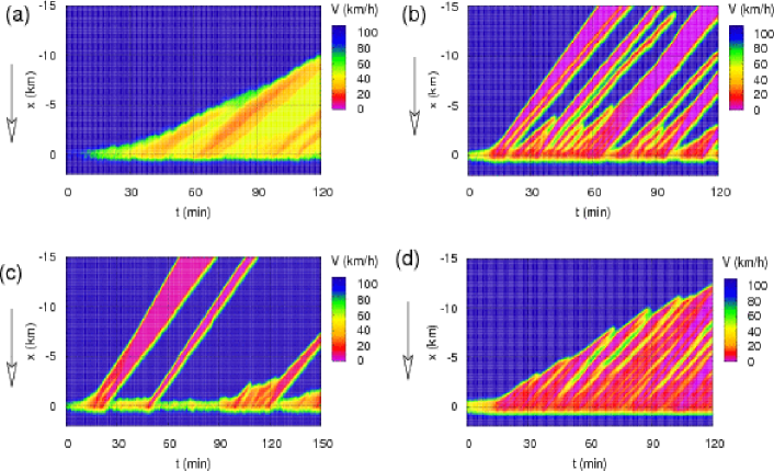
Figure 9: Traffic patterns produced by the KK model in the open system with an on-ramp (merging length 600 m). (a) Inflow $Q_{\rm in}=2100\,\mathrm{vehicles/h}$ and ramp flow $Q_{\rm rmp}=150\,\mathrm{vehicles/h}$; (b) $Q_{\rm in}=2050\,\mathrm{vehicles/h}$, $Q_{\rm rmp}=550\,\mathrm{vehicles/h}$ (c) $Q_{\rm in}=2250\,\mathrm{vehicles/h}$, $Q_{\rm rmp}=320\,\mathrm{vehicles/h}$, and (d) $Q_{\rm in}=1350\,\mathrm{vehicles/h}$, $Q_{\rm rmp}=750\,\mathrm{vehicles/h}$.

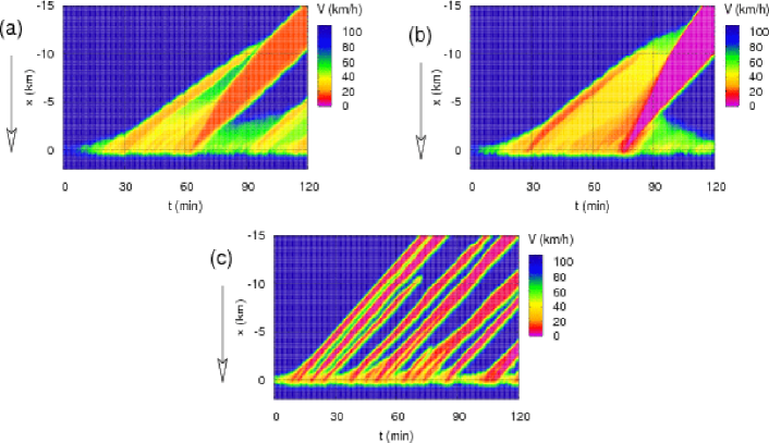
Figure 10: (a) “Moving synchronized pattern” (for $Q_{\rm in}=2120\,\mathrm{vehicles/h}$ and $Q_{\rm rmp}=200\,\mathrm{vehicles/h}$), and (b) “dissolving general pattern” (for $Q_{\rm in}=2150\,\mathrm{vehicles/h}$ and $Q_{\rm rmp}=250\,\mathrm{vehicles/h}$), simulated with the KK micro-model. The plot (c) shows the pinch effect for $Q_{\rm in}=1950\,\mathrm{vehicles/h}$, $Q_{\rm rmp}=500\,\mathrm{vehicles/h}$, and the synchronization distance parameter $k=1$, for which the KK micro-model is reduced to a model with a unique fundamental diagram.

4.2 Three-phase models

To facilitate a direct comparison of two- and three-phase models, we have simulated the same traffic system with two models implementing three-phase traffic theory, namely the cellular automaton of Kerner (2004) and the continuous-in space model proposed by Kerner and Klenov (2002). In the following, we will focus on the continuous model and refer to it as KK micro-model. It is formulated in terms of a coupled iterated map, i.e., the locations and velocities of the vehicles are continuous, but the updates of the locations and velocities occur in discrete time steps.

To calculate one longitudinal velocity update, 19 update rules have to be applied (see Kerner (2004), Eqs. (16.41), (16.44)-(16.48), and the 13 equations of Table 16.5 therein). Besides the vehicle length, the KK micro-model has 11 parameters and two functions containing five more constants: The desired velocity $v_{\rm free}$, the time $\tau$ which represents both, the update time step and the minimum time gap, the maximum acceleration $a$, the deceleration $b$ for determining the “safe” velocity, the synchronization range parameter $k$ indicating the ratio between maximum and minimum synchronized flow under stationary conditions at a certain density, the dimensionless sensitivity $\phi_{0}$ with respect to velocity differences, a threshold acceleration $\delta$ that defines, whether the vehicle is in the state of “nearly constant speed”, and three probabilities $p_{1}$, $p_{a}$, and $p_{b}$ defining acceleration noise and a slow-to-start rule. Additionally, the stochastic part of the model contains the two probability functions $p_{0}(v)=0.575+0.125\min(1,0.1v)$ (with $v$ in units of m/s), and $p_{2}(v)=0.48$, if $v\leq 15\,\mathrm{m/s}$, otherwise $p_{2}(v)=0.8$. The KK micro-model includes further rules for lane changes and merges.

We have implemented the longitudinal update rules according to the formulation in Kerner (2004), Section 16.3, and used the parameters from this reference as well. Since we are interested in the longitudinal dynamics, we will use the simpler merging rule applied already to the IDM in Sec. 4.1.2 of this paper. To test the implementation, we have simulated the open on-ramp system with a merging length of 600 m, as in the other simulations. This essentially produced the phase diagram and traffic patterns depicted in Fig. 18.1 of Kerner (2004). (Due to the simplified merging rule assumed here, the agreement is good, but not exact.)

Figure 9 shows the patterns which are crucial to compare the KK micro-model with the two-phase models of the previous section. We observe that the WSP pattern (diagram (a)), the pinch effect (diagram (b)), and the OCT (diagram (d)) are essentially equivalent with those of the IDM (Fig. 6) or the GKT model for parameter set 2 (see Fig. 4), but with the exception of the missing HCT states. Furthermore, the pattern shown in diagram (c) resembles the triggered stop-and-go traffic (TSG) displayed in Fig. 3(b). Some differences, however, remain:

• The oscillation frequencies of oscillatory patterns of the KK micro-model are smaller than those of the IDM, and often closer to reality. However, generalizing the IDM by considering reactions to next-nearest neighbors (Treiber et al., 2006b) increases the frequencies occurring in the IDM to realistic values. Note that the dynamics in the KK micro-model depends on next-nearest vehicles as well, so this may be an important aspect for microscopic traffic models to be realistic.

• The “moving synchronized patterns” in Fig. 10(a) (see also Fig. 18.1(d) in Kerner (2004)) differ from all other patterns in that their downstream fronts (where vehicles leave the jams) and the internal structures within the congested state propagate upstream at different velocities. Within the KK micro-model, the propagation velocity of structures in congested traffic may even exceed 40 km/h (see, for example, Fig. 18.27 in (Kerner, 2004)), while there is no empirical evidence of this. Observations rather suggest that the downstream front of congestion patterns is either stationary or propagates at a characteristic speed (see stylized fact 4 in Sec. 2.2).

• Another pattern which is sometimes produced by three-phase models is the “dissolving general pattern” (DGP), where an emerging wide moving jam leads to the dissolution of synchronized traffic (Fig. 10(b), see also Fig. 18.1(g) in  Kerner (2004)). So far, we have not found any evidence for such a pattern in our extensive empirical data sets. Congested traffic normally dissolves in different ways (see stylized facts 4 and 5).

Finally, we observe that the time gap $T$ of the KK micro-model in stationary car-following situations can adopt a range given by $\tau\leq T\leq k\tau$, where $k$ is the synchronization distance factor. By setting $k=1$, the KK micro-model becomes a conventional two-phase model. When simulating the on-ramp scenario for the KK micro-model with $k=1$, we essentially found the same patterns (see Fig. 10(c) for an example). This suggests that there is actually no need of going beyond the simpler class of two-phase models with a unique fundamental diagram.

4.3 Different mechanisms producing the pinch effect

While the very first publications on the phase diagram of traffic states did not report a pinch effect (or “general pattern”), the previous sections of this paper have shown that this traffic pattern can be simulated by two-phase models, if the model parameters are suitably chosen. It also appears that nonstationary perturbations at a bottleneck (which may, for example, result from frequent lane changes due to weaving flows) support the occurrence of a pinch effect. This suggests to take a closer look at mechanisms, which produce this effect. We have identified three possible explanations, which are discussed in the following. In reality, one may also have a combination of these mechanisms.

4.3.1 Mechanism I: metastability and depletion effect

This mechanism is the one proposed by three-phase traffic theory. The starting point is a region with metastable congested (but flowing) traffic behind a bottleneck, while sufficiently large perturbations trigger small oscillations in the density or velocity that grow while propagating upstream. When they become fully developed jams, the outflow from the oscillations decreases, which is modeled by some sort of slow-to-start rule: Once stopped or forced to drive at very low velocity, drivers accelerate more slowly, or keep a longer time gap than they would do when driving at a higher velocity. In the KK micro-model, this effect is implemented by using velocity-dependent stochastic deceleration probabilities $p_{0}(v)$ and $p_{2}(v)$. Other implementations of this effect are possible as well, such as the memory effect (Treiber and Helbing, 2003), or a driving style that depends on the local velocity variance (Treiber et al., 2006b). Even the parameters $s_{0}$ and $s_{1}$ of the IDM can be used to reflect this effect.

In any case, as soon as the outflow from large jams becomes smaller than that from small jams, most of the latter will eventually dissolve, resulting in only a few “wide moving jams”. We call this the “depletion effect”.

4.3.2 Mechanism II: convective string instability

A typical feature of the pinch effect are small perturbations that grow to fully developed moving jams. Therefore, it is expected that (linear or nonlinear) instabilities of the traffic flow play an essential role. However, another characteristic feature of the pinch effect is a stationary congested region near the bottleneck, called the pinch region (Kerner, 1998).

The simultaneous observation of the stationary pinch region and growing perturbations upstream of it can be naturally explained by observing that, in spatially extended open systems (such as traffic systems), there are two different types of string instability (Huerre and Monkewitz, 1990; Kesting and Treiber, 2008b). For the first type, an absolute instability, the perturbations will eventually spread over the whole system. A pinch region, however, can only exist if the growing perturbations propagate away from the on-ramp (in the upstream direction), while they do not “infect” the bottleneck region itself. This corresponds to the second type of string instability called “convective instability”.

Figure 11 illustrates convectively unstable traffic by a simulation of the bottleneck system with the model of Gipps (1981): Small perturbations caused by the merging maneuvers near the on-ramp at $x=10\,\mathrm{km}$ grow only in the upstream direction and eventually transform to wide jams a few kilometers upstream. The IDM simulations of Fig. 6 show this mechanism as well.

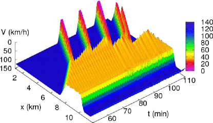
Figure 11: Simulation of the on-ramp system with the Gipps model showing the pinch effect. The parameters $v_{0}$, $a$, $b$ of this model have the same meaning as for the IDM and have been set to the same values (see main text). The update time $\Delta t$ (playing also the role of the time gap) has been set to $\Delta t=1.2\,\mathrm{s}$.

The concept of convective instability, which has been introduced into the context of traffic modeling already some years ago (Helbing et al., 1999), is in agreement empirical evidence. It has been observed that, in extended congested traffic, small perturbations or oscillations may grow while propagating upstream, whereas congested traffic is relatively stationary in the vicinity of the bottleneck (Kerner, 2004; Mauch and Cassidy, 2002; Smilowitz et al., 1999; Zielke et al., 2008). However, the congestion pattern emanating from the “pinch region” is not necessarily a fully developed “general pattern” in the sense that it includes a pinch region, small jams, and a transition to wide jams (Kerner, 2004). In fact, the pinch region is also observed as part of congestion patterns that include neither wide jams nor a significant number of merging events, see Fig. 1(a) for an example. This can be understood by assuming that the mechanisms leading to the pinch region and to wide jams are essentially independent from each other. One could therefore explain the pinch region by the convective instability, and the transition from small to wide jams by the depletion effect (see Sec. 4.3.1).

4.3.3 Mechanism III: locally increased stability

A third mechanism leading to similar results as the previous mechanisms comes into play at intersections and junctions, where off-ramps are located upstream of on-ramps (which corresponds to the usual freeway design). Figure 12(a) illustrates this mechanism for the GKT model and the parameter set 1 in Table 1. The existence of a stationary and essentially homogeneous pinch region and a stop-and-go pattern further upstream can be explained, assuming that the inflow $Q_{\rm rmp,on}$ from the on-ramp (located downstream) must be sufficiently large such that a HCT or OCT state would be produced when simulating this on-ramp alone. Furthermore, the outflow $Q_{\rm rmp,off}$ from the off-ramp must be such that an effective on-ramp of inflow

$$Q_{\rm rmp,eff}=Q_{\rm rmp,on}-Q_{\rm rmp,off}$$ (2)

would produce a TSG state or an OCT state with a larger wavelength.

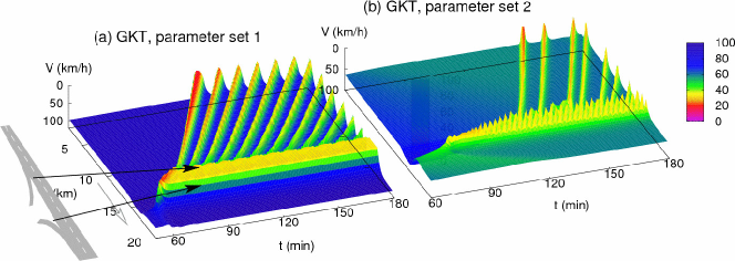
Figure 12: Congested traffic at a combination of an off-ramp with an on-ramp, simulated with the GKT model. The locally increased stability between the ramps supports the pinch and depletion effects, leading to a composite pattern consisting of a pinch region, narrow jams, and wide moving jams (see main text for details).

Figure 12(b) shows a simulation of an off-ramp-on-ramp scenario with the GKT model and parameter set 2 in Table 1. Notice that, for the parameters chosen, a pinch effect is not possible at an isolated on-ramp without a previous off-ramp (see Fig. 3). In Fig. 12(b), the on-ramp produces an OCT pattern, and the effective ramp flows according to Eq. (2) implies TSG traffic (or OCT with larger oscillation periods). The difference between the oscillation periods of the congestion pattern upstream of the on-ramp and upstream of the off-ramp leads to merging phenomena which are similar to those caused by the depletion effect. Notice that the existence of the depletion effect in congestion patterns forming behind intersections depends not only on the chosen traffic model and its parameters, but also on the traffic volume and the intersection design. This is in agreement with observations showing that some intersections tend to produce the full composite pattern consisting of the pinch region, narrow jams, and wide jams, while wide moving jams are missing at others (Kerner, 2004; Schönhof and Helbing, 2007). Furthermore, a pinch effect is usually not observed at flow-conserving bottlenecks (Schönhof and Helbing, 2007), and often not at separated on-ramps (see the traffic video at http://www.trafficforum.org/stopandgo).

Table 2: Overview of the main controversial traffic phenomena and their possible explanations. The term “three-phase model” has been used for models that are consistent with Kerner’s theory, while two-phase models are conventional models that can display traffic instabilities such as second-order macroscopic models and most car-following models (see Sec. 4 for details).

Phenomenon	Possible Mechanism	Examples and Models
Pinch region at a bottleneck; small jams further upstream	1. Convective instability or metastability	(i) Three-phase models (ii) Two-phase models with appropriate parameters
	2. Local change of stability and capacity	Off-ramp-on-ramp combinations
Transition from small to wide jams	1. Depletion mechanism	Slow-to-start rule and other forms of intra-driver variability
	2. Merging mechanism	Different group velocities of the small waves
Homogeneous congested traffic at low densities	Maximum flow is metastable or stable	Two- and three-phase models with suitable parameters
Homogeneous congested traffic at high densities	Restabilization	Severe bottleneck simulated with a two-phase model with appropriate parameters

4.4 Summary of possible explanations

Table 2 gives an overview of mechanisms producing the observed spatiotemporal phenomena listed in Sec. 2.2. So far, these have been either considered incompatible with three-phase models or with two-phase models having a fundamental diagram. It is remarkable that the main controversial observation — the occurrence of the pinch effect or general pattern — is not only compatible with three-phase models, but can also be produced with conventional two-phase models. For both model classes, this can be demonstrated with macroscopic, microscopic, and cellular automata models, if models and parameters are suitably chosen.

5 Conclusions

It appears that some of the current controversy in the area of traffic modeling arises from the different definitions of what constitutes a traffic phase. In the context of three-phase traffic theory, the definition of a phase is oriented at equilibrium physics, and in principle, it should be able to determine the phase based on local criteria and measurements at a single detector. Within three-phase traffic theory, however, this goal is not completely reached: In order to distinguish between “moving synchronized patterns” and wide moving jams, which look alike, one needs the additional nonlocal criterium of whether the congestion pattern propagates through the next bottleneck area or not (Schönhof and Helbing, 2007, 2009). In contrast, the alternative phase diagram approach is oriented at systems theory, where one tries to distinguish different kinds of elementary congestion patterns, which may be considered as non-equilibrium phases occurring in non-homogeneous systems (containing bottlenecks). These traffic patterns are distinguished into localized or spatially extended, moving or stationary (“pinned”), and spatially homogeneous or oscillatory patterns. These patterns can be derived from the stability properties of conventional traffic models exhibiting a unique fundamental diagram and unstable and/or metastable flows under certain conditions. Models of this class, sometimes also called two-phase models, include macroscopic and car-following models as well as cellular automata.

As key result of our paper we have found that features, which are claimed to be consistent with three-phase traffic theory only, can also be explained and simulated with conventional models, if the model parameters are suitably specified. In particular, if the parameters are chosen such that traffic at maximum flow is (meta-)stable and the density range for unstable traffic lies completely on the “congested” side of the fundamental diagram, we find the “widening synchronized pattern” (WSP), which has not been discovered in two-phase models before. Furthermore, the models can be tuned such that no homogeneous congested traffic (HCT) exists for strong bottlenecks. Conversely, we have shown that almost the same kinds of patterns, which are produced by two-phase models, are also found for models developed to reproduce three-phase traffic theory (such as the KK micro-model). Moreover, when the KK micro-model is simulated with parameters for which it turns into a model with a unique fundamental diagram, it still displays very similar results. Therefore, the difference between so-called two-phase and three-phase models does not seem to be as big as the current scientific controversy suggests.

For many empirical observations, we have found several plausible explanations (compatible and incompatible ones), which makes it difficult to determine the underlying mechanism which is actually at work. In our opinion, convective instability is a likely reason for the occurence of the pinch effect (or the general pattern), but at intersections with large ramp flows, the effect of off- and on-ramp combinations seems to dominate. To explain the transition to wide moving jams, we favour the depletion effect, as the group velocities of structures within congested traffic patterns are essentially constant. For the wide scattering of flow-density data, all three mechanisms of Table 2 do probably play a role. Clearly, further observations and experiments are necessary to confirm or reject these interpretations, and to exclude some of the alternative explanations. It seems to be an interesting challenge for the future to devise and perform suitable experiments in order to finally decide between the alternative explanation mechanisms.

In our opinion, the different congestion patterns produced by three-phase traffic theory and the alternative phase diagram approach for models with a fundamental diagram share more commonalities than differences. Moreover, according to our judgement, three-phase models do not explain more observations than the simpler two-phase models (apart maybe from the fluctuations of “synchronized flow”, which can, for example, be explained by the heterogeneity of driver-vehicle units). The question is, therefore, which approach is superior over the other. To decide this, the quality of models should be judged in a quantitative way, applying the following established standard procedure (Greene, 2008; Diebold, 2003):

• As a first step, mathematical quality functions must be defined. Note that the proper selection of these functions (and the relative weight that is given to them) depends on the purpose of the model.

• The crucial step is the statistical comparison of the competing models based on a new, but representative set of traffic measurements, using model parameters determined in a previous calibration step. Note that, due to the problem of over-fitting (i.e. the risk of fitting of noise in the data), a high goodness of fit in the calibration step does not necessarily imply a good fit of the new data set, i.e. a high predictive power (Brockfeld et al., 2003, 2004).

• The goodness of fit should be judged with established statistical methods, for example with the adjusted R-value or similar concepts considering the number of model parameters (Greene, 2008; Diebold, 2003). Given the same correlation with the data, a model containing a few parameters has a higher explanatory power than a model with many parameters.

Given a comparable predictive power of two models, one should select the simpler one according to Einstein’s principle that a model should be as simple as possible, but not simpler. If one has to choose between two equally performing models with the same number of parameters, one should use the one which is easier to interpret, i.e. a model with meaningful and independently measurable parameters (rather than just fit parameters). Furthermore, the model should not be sensitive to variations of the model parameters within the bounds of their confidence intervals. Applying this benchmarking process to traffic modeling will hopefully lead to an eventual convergence of explanatory concepts in traffic theory.

Acknowledgements

The authors would like to thank the Hessisches Landesamt für Straßen- und Verkehrswesen and the Autobahndirektion Südbayern for providing the freeway data shown in Figs. 1 and 2. They are furthermore grateful to Eddie Wilson for sharing the data set shown in Fig. 13, and to Anders Johansson for generating the plots from his data.

Appendix A Wide scattering of congested flow–density data

The discussion around three-phase traffic theory is directly related with the wide scattering of flow-density data within synchronized traffic flows. However, it deserves to be mentioned that the discussion around traffic theories has largely neglected the fact that empirical measurements of wide moving jams show a considerable amount of scattering as well (see, e.g. Fig. 15 of Treiber et al. (2000a)), while theoretically, one expects to find a “jam line” (Kerner, 2004). This suggests that wide scattering is actually not a specific feature of synchronized flow, but of congested traffic in general. While this questions the basis of three-phase traffic theory to a certain extent, particularly as it is claimed that wide scattering is a distinguishing feature of synchronized flows as compared to wide moving jams, the related car-following models (Kerner and Klenov, 2002), cellular automata (Kerner et al., 2002; Jiang and Wu, 2005), and macroscopic models (Jiang et al., 2007) build in dynamical mechanisms generating such scattering as one of their key features (Siebel and Mauser, 2006). In other models, particularly those with a fundamental diagram, this scattering is a simple add-on (and partly a side effect of the measurement process, see Sec. 2.1). It can be reproduced, for example, by considering heterogeneous driver-vehicle populations in macroscopic models (Wagner et al., 1996; Krauss et al., 1997; Banks, 1999; Treiber and Helbing, 1999; Hoogendoorn and Bovy, 2000) or car-following models (Nishinari et al., 2003; Ossen et al., 2007; Igarashi et al., 2005; Kesting and Treiber, 2008a), by noise terms (Treiber et al., 2006b), or slowly changing driving styles (Treiber and Helbing, 2003; Treiber et al., 2006a).

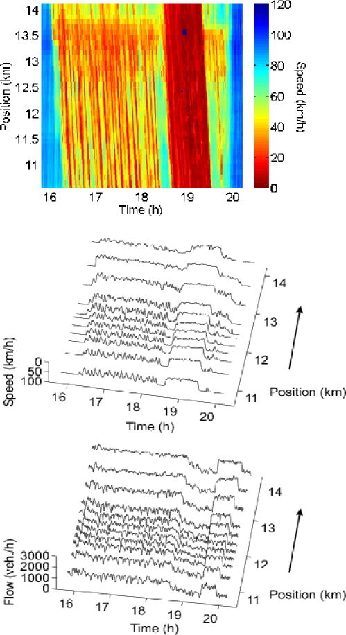
Figure 13: Homogeneous congested traffic on the high-coverage section of the British freeway M42 ATM (averaged over 3 running lanes) (Wilson, 2008b). Note that no interpolation or smoothing was applied to the data measured on November 27, 2008. The three-dimensional plots of the vehicle speed and the flow show measurements of each fifth detector only, otherwise the plots would have been overloaded. There is no clear evidence that perturbations in the vehicle speed or flow would grow upstream, i.e. against the flow direction that is indicated by arrows.

Appendix B Discussion of homogeneous congested traffic

For strong bottlenecks (typically caused by accidents), empirical evidence regarding the existence of homogeneous congested traffic has been somewhat ambiguous so far. On the one hand, when applying the adaptive smoothing method to get rid of noise in the data (Treiber and Helbing, 2002), the spatiotemporal speed profile looks almost homogeneous, even when the same smoothing parameters are used as for the measurement of the other traffic patterns, e.g. oscillatory ones (Schönhof and Helbing, 2007). On the other hand, it was claimed that data of the flow measured at freeway cross sections show an oscillatory behavior (Kerner, 2008). These oscillations typically have small wavelengths, which can have various origins: (1) They can result from the heterogeneity of driver-vehicle units, particularly their time gaps, which is known to cause a wide scattering of congested flow-density data (Nishinari et al., 2003). (2) They could as well result from problems in maintaining low speeds, as the gas and break pedals are difficult to control. (3) They may also be a consequence of perturbations, which can easily occur when traffic flows of several lanes have to merge in a single lane, as it is usually the case at strong bottlenecks. According to stylized fact 6, all these perturbations are expected to propagate upstream at the speed $c_{\rm cong}$. In order to judge whether the pattern is to be classified as oscillatory congested traffic or homogeneous congested traffic, one would have to determine the sign of the growth rate of perturbations, i.e. whether large perturbations grow bigger or smaller while travelling upstream.

Recent traffic data of high spatial and temporal resolution suggest that homogeneous congested traffic states do exist (see Fig. 13), but are very rare. For the conclusions of this paper and the applicability of the phase diagram approach, however, it does not matter whether homogeneous congested traffic actually exists or not. This is, because many models with a fundamental diagram can be calibrated in a way that either generates homogeneous patterns for high bottleneck strengths or not (see Sec. 4).

References

- Appert and Santen (2001) Appert, C., Santen, L., 2001. Boundary induced phase transitions in driven lattice gases with metastable states. Physical Review Letters 86 (12), 2498–1501.
- Aw and Rascle (2000) Aw, A., Rascle, M., 2000. Resurrection of ”second order” models of traffic flow. SIAM Journal on Applied Mathematics 60 (3), 916–938.
- Bando et al. (1995) Bando, M., Hasebe, K., Nakanishi, K., Nakayama, A., Shibata, A., Sugiyama, Y., 1995. Phenomenological study of dynamical model of traffic flow. Journal de Physique I France 5 (11), 1389-1399.
- Banks (1999) Banks, J. H., 1999. Investigation of some characteristics of congested flow. Transportation Research Record 1678, 128–134.
- Belomestny et al. (2003) Belomestny, D., Jentsch, V., Schreckenberg, M., 2003. Completion and continuation of nonlinear traffic time series: a probabilistic approach. Journal of Physics A: Mathematical and General 36 (45), 11369–11383.
- Bertini et al. (2004) Bertini, R., Lindgren, R., Helbing, D., Schönhof, M., 2004. Empirical analysis of flow features on a German autobahn. In: Transportation Research Board 83rd Annual Meeting, Washington DC. Washington, D.C., available at Arxiv eprint cond-mat/0408138.
- Brockfeld et al. (2004) Brockfeld, E., Kühne, R. D., Wagner, P., 2004. Calibration and validation of microscopic traffic flow models. Transportation Research Record 1876, 62–70.
- Brockfeld et al. (2003) Brockfeld, E., Kühne, R. D., Skabardonis, A., Wagner, P., 2004. Toward benchmarking of microscopic traffic flow models. Transportation Research Record 1852, 124–129.
- Cassidy and Windower (1995) Cassidy, M. J., Windower, J., 1995. Methodology for assessing dynamics of freeway traffic flow. Transportation Research Record 1484, 73–79.
- Coifman (2002) Coifman, B., 2002. Estimating travel times and vehicle trajectories on freeways using dual loop detectors. Transportation Research Part A 36 (4), 351–364.
- Daganzo (1995) Daganzo, C. F., 1995. Requiem for second-order fluid approximations of traffic flow. Transportation Research Part B 29 (4), 277–286.
- Diebold (2003) Diebold, F., 2003. Elements of Forecasting. South-Western Publishing, Cincinatti.
- Gipps (1981) Gipps, P. G., 1981. A behavioural car-following model for computer simulation. Transportation Research Part B 15 (2), 105–111.
- Greene (2008) Greene, W. H., 2008. Econometric Analysis, particularly Chap. 7.4: Model selection criteria. Prentice Hall, Upper Saddle River, NJ.
- Helbing (1996) Helbing, D., 1996. Gas-kinetic derivation of Navier-Stokes-like traffic equations. Physical Review E 53 (3), 2366–2381.
- Helbing (2001) Helbing, D., 2001. Traffic and related self-driven many-particle systems. Reviews of Modern Physics 73 (4), 1067–1141.
- Helbing et al. (1999) Helbing, D., Hennecke, A., Treiber, M., 1999. Phase diagram of traffic states in the presence of inhomogeneities. Physical Review Letters 82 (21), 4360–4363.
- Helbing and Johansson (2009) Helbing, D., Johansson, A. F., 2009. On the controversy around Daganzo’s requiem for and Aw-Rascle’s resurrection of second-order traffic flow models. European Physical Journal B 69 (4), 549–562.
- Helbing and Tilch (2009) Helbing, D., Tilch, B., 2009. A power law for the duration of high-flow states and its interpretation from a heterogeneous traffic flow perspective. The European Physical Journal B 68 (4), 577–586.
- Helbing and Treiber (2002) Helbing, D., Treiber, M., 2002. Critical discussion of ”synchronized flow”. Cooper@tive Tr@nsport@tion Dyn@mics 1, 2.1–2.24, (Internet Journal, www.TrafficForum.org/journal).
- Helbing et al. (2009) Helbing, D., Treiber, M., Kesting, A., Schönhof, M., 2009. Theoretical vs. empirical classification and prediction of congested traffic states. The European Physical Journal B 69 (4), 583–598.
- Hoogendoorn and Bovy (2000) Hoogendoorn, S., Bovy, P., 2000. Gas-kinetic modeling and simulation of pedestrian flows. Transportation Research Record 1710, 28–36.
- Huerre and Monkewitz (1990) Huerre, P., Monkewitz, P., 1990. Local and global instabilities in spatially developing flows. Annual Review of Fluid Mechanics 22 (1), 473–537.
- Igarashi et al. (2005) Igarashi, K., Takeda, K., Itakura, F., Abut, H., 2005. Is our driving behavior unique? In: DSP for In-Vehicle and Mobile Systems. Springer, pp. 257–274.
- Jiang et al. (2007) Jiang, R., Hu, M., Jia, B., Wang, R., Wu, Q., 2007. Spatiotemporal congested traffic patterns in macroscopic version of the Kerner–Klenov speed adaptation model. Physics Letters A 365 (1-2), 6–9.
- Jiang et al. (2001) Jiang, R., Wu, Q., Zhu, Z., 2001. Full velocity difference model for a car-following theory. Physical Review E 64 (1), 017101.
- Jiang and Wu (2005) Jiang, R., Wu, Q.-S., 2005. Toward an improvement over Kerner-Klenov-Wolf three-phase cellular automaton model. Physical Review E 72 (6), 067103.
- Kerner (1998) Kerner, B., 1998. Experimental features of self-organization in traffic flow. Physical Review Letters 81, 3797–3800.
- Kerner (2002) Kerner, B., 2002. Empirical macroscopic features of spatio-temporal traffic patterns at highway bottlenecks. Physical Review E 65 (4), 046138.
- Kerner (2008) Kerner, B., 2008. A theory of traffic congestion at heavy bottlenecks. Journal of Physics A: Mathematical and General 41 (21), 215101.
- Kerner and Klenov (2002) Kerner, B., Klenov, S., 2002. A microscopic model for phase transitions in traffic flow. Journal of Physics A: Mathematical and General 35 (3), L31–L43.
- Kerner and Klenov (2006) Kerner, B., Klenov, S., 2006. Deterministic microscopic three-phase traffic flow models. Journal of Physics A: Mathematical and General 39 (8), 1775–1810.
- Kerner et al. (2002) Kerner, B., Klenov, S., Wolf, D., 2002. Cellular automata approach to three-phase traffic theory. Journal of Physics A: Mathematical and General 35 (47), 9971–10013.
- Kerner and Konhäuser (1993) Kerner, B., Konhäuser, P., 1993. Cluster effect in initially homogeneous traffic flow. Physical Review E 48 (4), R2335.
- Kerner and Rehborn (1996a) Kerner, B., Rehborn, H., 1996a. Experimental features and characteristics of traffic jams. Physical Review E 53 (2), 1297–1300.
- Kerner and Rehborn (1996b) Kerner, B., Rehborn, H., 1996b. Experimental properties of complexity in traffic flow. Physical Review E 53 (5), R4275–R4278.
- Kerner et al. (2001) Kerner, B., Rehborn, H., Aleksic, M., Haug, A., Lange, R., 2001. Online automatic tracing and forecasting of traffic patterns. Traffic Engineering and Control 42 (10), 345–350.
- Kerner (2004) Kerner, B. S., 2004. The Physics of Traffic: Empirical Freeway Pattern Features, Engineering Applications, and Theory. Springer, Heidelberg.
- Kesting and Treiber (2008a) Kesting, A., Treiber, M., 2008a. Calibrating car-following models by using trajectory data: Methodological study. Transportation Research Record: Journal of the Tranportation Research Board 2088, 148–156.
- Kesting and Treiber (2008b) Kesting, A., Treiber, M., 2008b. How reaction time, update time and adaptation time influence the stability of traffic flow. Computer-Aided Civil and Infrastructure Engineering 23 (2), 125–137.
- Krauss et al. (1997) Krauss, S., Wagner, P., Gawron, C., 1997. Metastable states in a microscopic model of traffic flow. Physical Review E 55 (5), 5597–5602.
- Krug (1991) Krug, J., 1991. Boundary-induced phase transitions in driven diffusive systems. Physical Review Letters 67 (14), 1882–1885.
- Lee et al. (1998) Lee, H., Lee, H., Kim, D., 1998. Origin of synchronized traffic flow on highways and its dynamic phase transition. Physical Review Letters 81 (5), 1130.
- Lee et al. (1999) Lee, H. Y., Lee, H. W., Kim, D., 1999. Dynamic states of a continuum traffic equation with on-ramp. Physical Review E 59 (5), 5101–5111.
- Lighthill and Whitham (1955) Lighthill, M., Whitham, G., 1955. On kinematic waves: II. A theory of traffic on long crowded roads. Proc. Roy. Soc. of London A 229 (1178), 317–345.
- Lindgren et al. (2006) Lindgren, R. V., Bertini, R. L., Helbing, D., Schönhof, M., 2006. Toward demonstrating the predictability of bottleneck activation on German autobahns. Transportation Research Record 1965, 12–22.
- Mauch and Cassidy (2002) Mauch, M., Cassidy, M. J., 2002. Freeway traffic oscillations: observations and predictions. In: Taylor, M. (Ed.), International Symposium of Traffic and Transportation Theory. Elsevier, Amsterdam.
- Muñoz and Daganzo (2002) Muñoz, J., Daganzo, C., 2002. Fingerprinting traffic from static freeway sensors. Cooperative Transportation Dynamics 1, 1–11, (Internet Journal, www.trafficforum.org/journal).
- Nishinari et al. (2003) Nishinari, K., Treiber, M., Helbing, D., 2003. Interpreting the wide scattering of synchronized traffic data by time gap statistics. Physical Review E 68 (6), 067101.
- Ossen et al. (2007) Ossen, S., Hoogendoorn, S. P., Gorte, B. G., 2007. Inter-driver differences in car-following: A vehicle trajectory based study. Transportation Research Record 1965, 121–129.
- Payne (1971) Payne, H., 1971. Models of Freeway Traffic and Control. Simulation Councils, Inc.
- Popkov et al. (2001) Popkov, V., Santen, L., Schadschneider, A., Schütz, G. M., 2001. Empirical evidence for a boundary-induced nonequilibrium phase transition. Journal of Physics A: Mathematical General 34 (6), L45–L52.
- Richards (1956) Richards, P., 1956. Shock waves on the highway. Operations Research 4 (41), 42–51.
- Schönhof and Helbing (2007) Schönhof, M., Helbing, D., 2007. Empirical features of congested traffic states and their implications for traffic modeling. Transportation Science 41 (2), 1–32.
- Schönhof and Helbing (2009) Schönhof, M., Helbing, D., 2009. Critisism of three-phase traffic theory. Transporation Research Part B 43 (7), 784–797.
- Siebel and Mauser (2006) Siebel, F., Mauser, W., 2006. Synchronized flow and wide moving jams from balanced vehicular traffic. Physical Review E 73 (6), 66108.
- Smilowitz et al. (1999) Smilowitz, K., Daganzo, C., Cassidy, M., Bertini, R., 1999. Some observations of highway traffic in long queues. Transportation Research Record: Journal of the Transportation Research Board 1678, 225–233.
- Treiber and Helbing (1999) Treiber, M., Helbing, D., 1999. Macroscopic simulation of widely scattered synchronized traffic states. Journal of Physics A: Mathematical and General 32 (1), L17–L23.
- Treiber and Helbing (2002) Treiber, M., Helbing, D., 2002. Reconstructing the spatio-temporal traffic dynamics from stationary detector data. Cooperative Transportation Dynamics 1, 3.1–3.24, (Internet Journal, www.TrafficForum.org/journal).
- Treiber and Helbing (2003) Treiber, M., Helbing, D., 2003. Memory effects in microscopic traffic models and wide scattering in flow-density data. Physical Review E 68 (4), 046119.
- Treiber et al. (1999) Treiber, M., Hennecke, A., Helbing, D., 1999. Derivation, properties, and simulation of a gas-kinetic-based, non-local traffic model. Physical Review E 59 (1), 239–253.
- Treiber et al. (2000a) Treiber, M., Hennecke, A., Helbing, D., 2000a. Congested traffic states in empirical observations and microscopic simulations. Physical Review E 62 (2), 1805–1824.
- Treiber et al. (2000b) Treiber, M., Hennecke, A., Helbing, D., 2000b. Microscopic simulation of congested traffic. In: Helbing, D., Herrmann, H., Schreckenberg, M., Wolf, D. (Eds.), Traffic and Granular Flow ’99. Springer, Berlin, pp. 365–376.
- Treiber et al. (2006a) Treiber, M., Kesting, A., Helbing, D., 2006a. Delays, inaccuracies and anticipation in microscopic traffic models. Physica A 360 (1), 71–88.
- Treiber et al. (2006b) Treiber, M., Kesting, A., Helbing, D., 2006b. Understanding widely scattered traffic flows, the capacity drop, and platoons as effects of variance-driven time gaps. Physical Review E 74 (1), 016123.
- Treiber et al. (2010) Treiber, M., Kesting, A., Wilson, R. E., 2010. Reconstructing the traffic state by fusion of heterogenous data, Computer-Aided Civil and Infrastructure Engineering, accepted. Preprint physics/0900.4467.
- Wagner et al. (1996) Wagner, C., Hoffmann, C., Sollacher, R., Wagenhuber, J., Schürmann, B., 1996. Second-order continuum traffic flow model. Physical Review E 54 (5), 5073.
- Wagner and Nagel (2008) Wagner, P., Nagel, K., 2008. Comparing traffic flow models with different number of ‘phases’. The European Physical Journal B 63 (3), 315–320.
- Whitham (1974) Whitham, G., 1974. Linear and Nonlinear Waves. Wiley, New York.
- Wilson (2008a) Wilson, R., 2008a. Mechanisms for spatio-temporal pattern formation in highway traffic models. Philosophical Transactions of the Royal Society A 366 (1872), 2017–2032.
- Wilson (2008b) Wilson, R. E., 2008b. From inductance loops to vehicle trajectories. See e-print http://hdl.handle.net/1983/1162
- Zielke et al. (2008) Zielke, B., Bertini, R., Treiber, M., 2008. Empirical Measurement of Freeway Oscillation Characteristics: An International Comparison. Transportation Research Record 2088, 57–67.