Microscopic description of large-amplitude shape-mixing dynamics with inertial functions derived in local quasiparticle random-phase approximation

Abstract

On the basis of the adiabatic self-consistent collective coordinate method, we develop an efficient microscopic method of deriving the five-dimensional quadrupole collective Hamiltonian and illustrate its usefulness by applying it to the oblate-prolate shape coexistence/mixing phenomena in proton-rich ^68,70,72Se. In this method, the vibrational and rotational collective masses (inertial functions) are determined by local normal modes built on constrained Hartree-Fock-Bogoliubov states. Numerical calculations are carried out using the pairing-plus-quadrupole Hamiltonian including the quadrupole-pairing interaction within the two major-shell active model spaces both for neutrons and protons. It is shown that the time-odd components of the moving mean-field significantly increase the vibrational and rotational collective masses in comparison with the Inglis-Belyaev cranking masses. Solving the collective Schrödinger equation, we evaluate excitation spectra, quadrupole transitions and moments. Results of the numerical calculation are in excellent agreement with recent experimental data and indicate that the low-lying states of these nuclei are characterized as an intermediate situation between the oblate-prolate shape coexistence and the so-called $\gamma$ unstable situation where large-amplitude triaxial-shape fluctuations play a dominant role.

I Introduction

The major purpose of this paper is to develop an efficient microscopic method of deriving the five-dimensional (5D) quadrupole collective Hamiltonian Bohr and Mottelson (1998); Belyaev (1965); Kumar and Baranger (1967); Próchniak and Rohoziński (2009) and illustrate its usefulness by applying it to the oblate-prolate shape coexistence/mixing phenomena in proton-rich Se isotopes Fischer et al. (2003, 2000); Obertelli et al. (2009); Ljungvall et al. (2008). As is well known, the quadrupole collective Hamiltonian, also called the general Bohr-Mottelson Hamiltonian, contains six collective inertia masses (three vibrational masses and three rotational moments of inertia) as well as the collective potential. These seven quantities are functions of the quadrupole deformation variables $\beta$ and $\gamma$, which represent the magnitude and triaxiality of the quadrupole deformation, respectively. Therefore, we also call the collective inertial masses ‘inertial functions.’ They are usually calculated by means of the adiabatic perturbation treatment of the moving mean field Inglis (1954), and the version taking into account nuclear superfluidity Beliaev (1961) is called the Inglis-Belyaev (IB) cranking mass or the IB inertial function. Its insufficiency has been repeatedly emphasized, however (see e.g., Refs. Kumar (1974); Pomorski et al. (1977); Rohoziński et al. (1977); Dudek et al. (1980)). The most serious shortcoming is that the time-odd terms induced by the moving mean field are ignored, which breaks the self-consistency of the theory Baranger and Vénéroni (1978); Dobaczewski and Skalski (1981). In fact, one of the most important motives of constructing microscopic theory of large-amplitude collective motion was to overcome such a shortcoming of the IB cranking mass Baranger and Vénéroni (1978).

As fruits of long-term efforts, advanced microscopic theories of inertial functions are now available (see Refs. Villars (1977); Baranger and Vénéroni (1978); Goeke and Reinhard (1978); Rowe and Bassermann (1976); Marumori (1977); Libert et al. (1999); Dobaczewski and Skalski (1981); Pal et al. (1975); Walet et al. (1991); Almehed and Walet (2004); Marumori et al. (1980); Giannoni and Quentin (1980) for original papers and Refs. Dang et al. (2000); Matsuyanagi et al. (2010) for reviews). These theories of large-amplitude collective motion have been tested for schematic solvable models and applied to heavy-ion collisions and giant resonances Goeke and Reinhard (1978); Giannoni and Quentin (1980). For nuclei with pairing correlations, Dobaczewski and Skalski studied the quadrupole vibrational mass with use of the adiabatic time-dependent Hartree-Fock-Bogoliubov (ATDHFB) theory and concluded that the contributions from the time-odd components of the moving mean-field significantly increase the vibrational mass compared to the IB cranking mass Dobaczewski and Skalski (1981). Somewhat surprisingly, however, to the best of our knowledge, the ATDHFB vibrational masses have never been used in realistic calculations for low-lying quadrupole spectra of nuclei with superfluidity. For instance, in recent microscopic studies Nikšić et al. (2007, 2009); Li et al. (2009, 2010); Girod et al. (2009); Delaroche et al. (2010) by means of the 5D quadrupole Hamiltonian, the IB cranking formula are still used in actual numerical calculation for vibrational masses. This situation concerning the treatment of the collective kinetic energies is in marked contrast with the remarkable progress in microscopic calculation of the collective potential using modern effective interactions or energy density functionals (see Ref. Bender et al. (2003) for a review).

In this paper, on the basis of the adiabatic self-consistent collective coordinate (ASCC) method Matsuo et al. (2000), we formulate a practical method of deriving the 5D quadrupole collective Hamiltonian. The central concept of this approach is local normal modes built on constrained Hartree-Fock-Bogoliubov (CHFB) states Ring and Schuck (1980) defined at every point of the ($\beta,\gamma$) deformation space. These local normal modes are determined by the local QRPA (LQRPA) equation that is an extension of the well-known quasiparticle random-phase approximation (QRPA) to non-equilibrium HFB states determined by the CHFB equations. We therefore use an abbreviation ‘CHFB+LQRPA method’ for this approach. This method may be used in conjunction with any effective interaction or energy density functional. In this paper, however, we use, for simplicity, the pairing-plus-quadrupole (P+Q) force Bes and Sorensen (1969); Baranger and Kumar (1968a) including the quadrupole-pairing force. Inclusion of the quadrupole-pairing force is essential because it produces the time-odd component of the moving field Hinohara et al. (2006).

To examine the feasibility of the CHFB+LQRPA method, we apply it to the oblate-prolate shape coexistence/mixing phenomena in proton-rich ^68,70,72Se Fischer et al. (2003, 2000); Obertelli et al. (2009); Ljungvall et al. (2008); Rainovski et al. (2002); Palit et al. (2001). These phenomena are taken up because we obviously need to go beyond the traditional framework of describing small-amplitude vibrations around a single HFB equilibrium point to describe them; that is, they are very suitable targets for our purpose. We shall show in this paper that this approach successfully describes large-amplitude collective vibrations extending from the oblate to the prolate HFB equilibrium points (and vice versa). In particular, it will be demonstrated that we can describe very well the transitional region between the oblate-prolate shape coexistence and the $\gamma$ unstable situation where large-amplitude triaxial-shape fluctuations play a dominant role.

This paper is organized as follows. In Sec. II, we formulate the CHFB+LQRPA as an approximation of the ASCC method and derive the 5D quadrupole collective Hamiltonian. In Sec. III, we calculate the vibrational and rotational masses by solving the LQRPA equations, and discuss their properties in comparison with those calculated by using the IB cranking formula. In Sec. IV, we calculate excitation spectra, $B(E2)$, and spectroscopic quadrupole moments of low-lying states in ^68,70,72Se and discuss properties of the oblate-prolate shape coexistence/mixing in these nuclei. Conclusions are given in Sec. V.

II Microscopic derivation of the 5D quadrupole collective Hamiltonian

II.1 The 5D quadrupole collective Hamiltonian

Our aim in this section is to formulate a practical method of microscopically deriving the 5D quadrupole collective Hamiltonian Bohr and Mottelson (1998); Belyaev (1965); Kumar and Baranger (1967); Próchniak and Rohoziński (2009)

$${\cal H}_{\rm coll} =T_{\rm vib}+T_{\rm rot}+V(\beta,\gamma),$$ (1)

$$T_{\rm vib} =\frac{1}{2}D_{\beta\beta}(\beta,\gamma)\dot{\beta}^{2}+D_{\beta\gamma}(\beta,\gamma)\dot{\beta}\dot{\gamma}+\frac{1}{2}D_{\gamma\gamma}(\beta,\gamma)\dot{\gamma}^{2},$$ (2)

$$T_{\rm rot} =\frac{1}{2}\sum_{k=1}^{3}{\cal J}_{k}(\beta,\gamma)\omega^{2}_{k},$$ (3)

starting from an effective Hamiltonian for finite many-nucleon systems. Here, $T_{\rm vib}$ and $T_{\rm rot}$ denote the kinetic energies of vibrational and rotational motions, while $V(\beta,\gamma)$ represents the collective potential. The velocities of the vibrational motion are described in terms of the time-derivatives ($\dot{\beta}$, $\dot{\gamma}$) of the quadrupole deformation variables ($\beta$, $\gamma$) representing the magnitude and the triaxiality of the quadrupole deformation, respectively. The three components $\omega_{k}$ of the rotational angular velocity are defined with respect to the intrinsic axes associated with the rotating nucleus. The inertial functions for vibrational motions (vibrational masses), $D_{\beta\beta}$, $D_{\beta\gamma}$, and $D_{\gamma\gamma}$, and the rotational moments of inertia ${\cal J}_{k}$ are functions of $\beta$ and $\gamma$.

As seen in the recent review by Próchniak and Rohoziński Próchniak and Rohoziński (2009), there are numerous papers on microscopic approaches to the 5D quadrupole collective Hamiltonian; among them, we should quote at least early papers by Belyaev Belyaev (1965), Baranger-Kumar Baranger and Kumar (1968b); Kumar and Baranger (1968), Pomorski et al. Pomorski et al. (1977); Rohoziński et al. (1977), and recent papers by Girod et al. Girod et al. (2009), Nikšić et al. Nikšić et al. (2007, 2009), and Li et al. Li et al. (2009, 2010). In all these works, the IB cranking formula is used for the vibrational inertial functions. Below, we outline the procedure of deriving the vibrational and rotational inertial functions on the basis of the ASCC method.

II.2 Basic equations of the ASCC method

To derive the 5D quadrupole collective Hamiltonian ${\cal H}_{\rm coll}$ starting from a microscopic Hamiltonian $\hat{H}$, we use the ASCC method Matsuo et al. (2000); Hinohara et al. (2007). This method enables us to determine a collective submanifold embedded in the large-dimensional TDHFB configuration space. We can use this method in conjunction with any effective interaction or energy density functional to microscopically derive the collective masses taking into account time-odd mean-field effects. For our present purpose, we here recapitulate a two-dimensional (2D) version of the ASCC method. We suppose existence of a set of two collective coordinates $(q^{1},q^{2})$ that has a one-to-one correspondence to the quadrupole deformation variable set $(\beta,\gamma)$ and try to determine a 2D collective hypersurface associated with the large-amplitude quadrupole shape vibrations. We thus assume that the TDHFB states can be written on the hypersurface in the following form;

$$\left|\phi(\bm{q},\bm{p},\bm{\varphi},\bm{n})\right\rangle =e^{-i\sum_{\tau}\varphi^{(\tau)}\widetilde{N}^{(\tau)}}\left|\phi(\bm{q},\bm{p},\bm{n})\right\rangle$$

$$=e^{-i\sum_{\tau}\varphi^{(\tau)}\widetilde{N}^{(\tau)}}e^{i\hat{G}(\bm{q},\bm{p},\bm{n})}\left|\phi(\bm{q})\right\rangle,$$ (4)

with

$$\hat{G}(\bm{q},\bm{p},\bm{n})= \sum_{i=1,2}p_{i}\hat{Q}^{i}(\bm{q})+\sum_{\tau=n,p}n^{(\tau)}\hat{\Theta}^{(\tau)}(\bm{q}),$$ (5)

$$\hat{Q}^{i}(\bm{q}) =\hat{Q}^{A}(\bm{q})+\hat{Q}^{B}(\bm{q})$$

$$= \sum_{\alpha\beta}[Q^{A}_{\alpha\beta}(\bm{q})a^{\dagger}_{\alpha}a^{\dagger}_{\beta}+Q^{A\ast}_{\alpha\beta}(\bm{q})a_{\beta}a_{\alpha}$$

$$+Q^{B}_{\alpha\beta}(\bm{q})a^{\dagger}_{\alpha}a_{\beta}],$$ (6)

$$\hat{\Theta}^{(\tau)}(\bm{q}) =\sum_{\alpha\beta}[\Theta^{(\tau)A}_{\alpha\beta}(\bm{q})a^{\dagger}_{\alpha}a^{\dagger}_{\beta}+\Theta^{(\tau)A\ast}_{\alpha\beta}(\bm{q})a_{\beta}a_{\alpha}].$$ (7)

For a gauge-invariant description of nuclei with superfluidity, we need to parametrize the TDHFB state vectors, as above, not only by the collective coordinates $\bm{q}=(q^{1},q^{2})$ and conjugate momenta $\bm{p}=(p_{1},p_{2})$ but also by the gauge angles $\bm{\varphi}=(\varphi^{(n)},\varphi^{(p)})$ conjugate to the number variables $\bm{n}=(n^{(n)},n^{(p)})$ representing the pairing-rotational degrees of freedom (for both neutrons and protons). In the above equations, $\hat{Q}^{i}(\bm{q})$ and $\hat{\Theta}^{(\tau)}(\bm{q})$ are infinitesimal generators which are written in terms of the quasiparticle creation and annihilation operators $(a^{\dagger}_{\alpha},a_{\alpha})$ locally defined with respect to the moving-frame HFB states $\left|\phi(\bm{q})\right\rangle$. Note that the number operators are defined as $\widetilde{N}^{(\tau)}\equiv\hat{N}^{(\tau)}-N_{0}^{(\tau)}$ subtracting the expectation values $(N_{0}^{(n)},N_{0}^{(p)})$ of the neutron and proton numbers at $\left|\phi(\bm{q})\right\rangle$. In this paper, we use units with $\hbar=1$.

The moving-frame HFB states $\left|\phi(\bm{q})\right\rangle$ and the infinitesimal generators $\hat{Q}^{i}(\bm{q})$ are determined as solutions of the moving-frame HFB equation,

$$\delta\left\langle\phi(\bm{q})\right|\hat{H}_{M}(\bm{q})\left|\phi(\bm{q})\right\rangle=0,$$ (8)

and the moving-frame QRPA equations,

$$\delta \left\langle\phi(\bm{q})\right|[\hat{H}_{M}(\bm{q}),\hat{Q}^{i}(\bm{q})]-\frac{1}{i}\sum_{k}B^{ik}(\bm{q})\hat{P}_{k}(\bm{q})$$

$$+\frac{1}{2}\left[\sum_{k}\frac{\partial V}{\partial q^{k}}\hat{Q}^{k}(\bm{q}),\hat{Q}^{i}(\bm{q})\right]\left|\phi(\bm{q})\right\rangle=0,$$ (9)

$$\delta \left\langle\phi(\bm{q})\right|[\hat{H}_{M}(\bm{q}),\frac{1}{i}\hat{P}_{i}(\bm{q})]-\sum_{j}C_{ij}(\bm{q})\hat{Q}^{j}(\bm{q})$$

$$-\frac{1}{2}\left[\left[\hat{H}_{M}(\bm{q}),\sum_{k}\frac{\partial V}{\partial q^{k}}\hat{Q}^{k}(\bm{q})\right],\sum_{j}B_{ij}(\bm{q})\hat{Q}^{j}(\bm{q})\right]$$

$$-\sum_{\tau}\frac{\partial\lambda^{(\tau)}}{\partial q^{i}}\widetilde{N}^{(\tau)}\left|\phi(\bm{q})\right\rangle=0,$$ (10)

which are derived from the time-dependent variational principle. Here, $\hat{H}_{M}(\bm{q})$ is the moving-frame Hamiltonian given by

$$\hat{H}_{M}(\bm{q})=\hat{H}-\sum_{\tau}\lambda^{(\tau)}(\bm{q})\widetilde{N}^{(\tau)}-\sum_{i}\frac{\partial V}{\partial q^{i}}\hat{Q}^{i}(\bm{q})$$ (11)

and

$$C_{ij}(\bm{q})=\frac{\partial^{2}V}{\partial q^{i}\partial q^{j}}-\sum_{k}\Gamma_{ij}^{k}\frac{\partial V}{\partial q^{k}}$$ (12)

with

$$\Gamma_{ij}^{k}(\bm{q})=\frac{1}{2}\sum_{l}B^{kl}(\frac{\partial B_{li}}{\partial q^{j}}+\frac{\partial B_{lj}}{\partial q^{i}}-\frac{\partial B_{ij}}{\partial q^{l}}).$$ (13)

The infinitesimal generators $\hat{P}_{i}(\bm{q})$ are defined by

$$\hat{P}_{i}(\bm{q})\left|\phi(\bm{q})\right\rangle=i\frac{\partial}{\partial q^{i}}\left|\phi(\bm{q})\right\rangle,$$ (14)

with

$$\hat{P}_{i}(\bm{q})=i\sum_{\alpha\beta}[P_{i\alpha\beta}(\bm{q})a^{\dagger}_{\alpha}a^{\dagger}_{\beta}-P_{i\alpha\beta}^{\ast}(\bm{q})a_{\beta}a_{\alpha}],$$ (15)

and determined as solutions of the moving-frame QRPA equations.

The collective Hamiltonian is given as the expectation value of the microscopic Hamiltonian with respect to the TDHFB state:

$${\cal H}(\bm{q},\bm{p},\bm{n})= \left\langle\phi(\bm{q},\bm{p},\bm{n})\right|\hat{H}\left|\phi(\bm{q},\bm{p},\bm{n})\right\rangle$$

$$= V(\bm{q})+\sum_{ij}\frac{1}{2}B^{ij}(\bm{q})p_{i}p_{j}+\sum_{\tau}\lambda^{(\tau)}(\bm{q})n^{(\tau)},$$ (16)

where

$$V(\bm{q})= {\cal H}(\bm{q},\bm{p},\bm{n})\Big{\arrowvert}_{\bm{p}=\bm{0},\bm{n}={\textbf{0}}},$$ (17)

$$B^{ij}(\bm{q})= \frac{\partial^{2}{\cal H}}{\partial p_{i}\partial p_{j}}\Big{\arrowvert}_{\bm{p}=\bm{0},\bm{n}={\textbf{0}}},$$ (18)

$$\lambda^{(\tau)}(\bm{q})= \frac{\partial{\cal H}}{\partial n^{(\tau)}}\Big{\arrowvert}_{\bm{p}=\bm{0},\bm{n}={\textbf{0}}},$$ (19)

represent the collective potential, inverse of the collective mass, and the chemical potential, respectively. Note that the last term in Eq. (10) can be set to zero adopting the QRPA gauge-fixing condition, $d\lambda^{(\tau)}/dq^{i}=0$ Hinohara et al. (2007).

The basic equations of the ASCC method are invariant against point transformations of the collective coordinates ($q^{1},q^{2}$). The $B^{ij}(\bm{q})$ and $C_{ij}(\bm{q})$ can be diagonalized simultaneously by a linear coordinate transformation at each point of $\bm{q}=(q^{1},q^{2})$. We assume that we can introduce the collective coordinate system in which the diagonal form is kept globally. Then, we can choose, without losing generality and for simplicity, the scale of the collective coordinates $\bm{q}=(q^{1},q^{2})$ such that the vibrational masses become unity. Consequently, the vibrational kinetic energy in the collective Hamiltonian (16) is written as

$$T_{\rm vib}=\frac{1}{2}\sum_{i=1,2}(p_{i})^{2}=\frac{1}{2}\sum_{i=1,2}(\dot{q^{i}})^{2}.$$ (20)

II.3 CHFB+LQRPA equations

The basic equations of the ASCC method can be solved with an iterative procedure. This task was successfully carried out for extracting a one-dimensional (1D) collective path embedded in the TDHFB configuration space Hinohara et al. (2008, 2009). To determine a 2D hypersurface, however, the numerical calculation becomes too demanding at the present time. We therefore introduce practical approximations as follows: First, we ignore the curvature terms (the third terms in Eqs. (9) and (10)), which vanish at the HFB equilibrium points where $dV/dq^{i}=0$, assuming that their effects are numerically small. Second, we replace the moving-frame HFB Hamiltonian $\hat{H}_{M}(\bm{q})$ and the moving-frame HFB state $\left|\phi(q^{1},q^{2})\right\rangle$ with a CHFB Hamiltonian $\hat{H}_{\rm CHFB}(\beta,\gamma)$ and a CHFB state $\left|\phi(\beta,\gamma)\right\rangle$, respectively, on the assumption that the latters are good approximations to the formers.

The CHFB equations are given by

$$\delta\left\langle\phi(\beta,\gamma)\right|\hat{H}_{\rm CHFB}(\beta,\gamma)\left|\phi(\beta,\gamma)\right\rangle=0,$$ (21)

$$\hat{H}_{\rm CHFB}(\beta,\gamma)= \hat{H}-\sum_{\tau}\lambda^{(\tau)}(\beta,\gamma)\widetilde{N}^{(\tau)}$$

$$-\sum_{m=0,2}\mu_{m}(\beta,\gamma)\hat{D}^{(+)}_{2m}$$ (22)

with four constraints

$$\left\langle\phi(\beta,\gamma)\right|\hat{N}^{(\tau)}\left|\phi(\beta,\gamma)\right\rangle=N^{(\tau)}_{0},\quad(\tau=n,p)$$ (23)

$$\left\langle\phi(\beta,\gamma)\right|\hat{D}^{(+)}_{2m}\left|\phi(\beta,\gamma)\right\rangle=D^{(+)}_{2m},\quad(m=0,2)$$ (24)

where $\hat{D}^{(+)}_{2m}$ denotes Hermitian quadrupole operators, $\hat{D}_{20}$ and $(\hat{D}_{22}+\hat{D}_{2-2})/2$ for $m=0$ and 2, respectively (see Ref. Hinohara et al. (2008) for their explicit expressions). We define the quadrupole deformation variables ($\beta,\gamma$) in terms of the expectation values of the quadrupole operators:

$$\beta\cos\gamma =\eta D^{(+)}_{20}=\eta\left\langle\phi(\beta,\gamma)\right|\hat{D}^{(+)}_{20}\left|\phi(\beta,\gamma)\right\rangle,$$ (25)

$$\frac{1}{\sqrt{2}}\beta\sin\gamma =\eta D^{(+)}_{22}=\eta\left\langle\phi(\beta,\gamma)\right|\hat{D}^{(+)}_{22}\left|\phi(\beta,\gamma)\right\rangle,$$ (26)

where $\eta$ is a scaling factor (to be discussed in subsection III.1).

The moving frame QRPA equations, (9) and (10), then reduce to

$$\delta \left\langle\phi(\beta,\gamma)\right|[\hat{H}_{\rm CHFB}(\beta,\gamma),\hat{Q}^{i}(\beta,\gamma)]$$

$$-\frac{1}{i}\hat{P}_{i}(\beta,\gamma)\left|\phi(\beta,\gamma)\right\rangle=0,\quad\quad(i=1,2)$$ (27)

and

$$\delta \left\langle\phi(\beta,\gamma)\right|[\hat{H}_{\rm CHFB}(\beta,\gamma),\frac{1}{i}\hat{P}_{i}(\beta,\gamma)]$$

$$-C_{i}(\beta,\gamma)\hat{Q}^{i}(\beta,\gamma)\left|\phi(\beta,\gamma)\right\rangle=0.\quad\quad(i=1,2)$$ (28)

Here the infinitesimal generators, $\hat{Q}^{i}(\beta,\gamma)$ and $\hat{P}_{i}(\beta,\gamma)$, are local operators defined at $(\beta,\gamma)$ with respect to the CHFB state $\left|\phi(\beta,\gamma)\right\rangle$. These equations are solved at each point of $(\beta,\gamma)$ to determine $\hat{Q}^{i}(\beta,\gamma)$, $\hat{P}_{i}(\beta,\gamma)$, and $C_{i}(\beta,\gamma)=\omega_{i}^{2}(\beta,\gamma)$. Note that these equations are valid also for regions with negative curvature ($C_{i}(\beta,\gamma)<0$) where the QRPA frequency $\omega_{i}(\beta,\gamma)$ takes an imaginary value. We call the above equations ‘local QRPA (LQRPA) equations’. There exist more than two solutions of LQRPA equations (27) and (28), and we need to select relevant solutions. A useful criterion for selecting two collective modes among many LQRPA modes will be given in subsection III.3 with numerical examples. Concerning the accuracy of the CHFB+LQRPA approximation, some arguments will be given in subsection III.6.

II.4 Derivation of the vibrational masses

Once the infinitesimal generators $\hat{Q}^{i}(\beta,\gamma)$ and $\hat{P}_{i}(\beta,\gamma)$ are obtained, we can derive the vibrational masses appearing in the 5D quadrupole collective Hamiltonian (1). We rewrite the vibrational kinetic energy $T_{\rm vib}$ given by Eq. (20) in terms of the time-derivatives, $\dot{\beta}$ and $\dot{\gamma}$, of the quadrupole deformation variables in the following way. We first note that an infinitesimal displacement of the collective coordinates $(q^{1},q^{2})$ brings about a corresponding change,

$$dD^{(+)}_{2m}= \sum_{i=1,2}\frac{\partial D^{(+)}_{2m}}{\partial q^{i}}dq^{i},\quad\quad(m=0,2),$$ (29)

in the expectation values of the quadrupole operators. The partial derivatives can be easily evaluated as

$$\frac{\partial D^{(+)}_{20}}{\partial q^{i}}= \frac{\partial}{\partial q^{i}}\left\langle\phi(\beta,\gamma)\right|\hat{D}^{(+)}_{20}\left|\phi(\beta,\gamma)\right\rangle$$

$$= \left\langle\phi(\beta,\gamma)\right|[\hat{D}^{(+)}_{20},\frac{1}{i}\hat{P}_{i}(\beta,\gamma)]\left|\phi(\beta,\gamma)\right\rangle,$$ (30)

$$\frac{\partial D^{(+)}_{22}}{\partial q^{i}}= \frac{\partial}{\partial q^{i}}\left\langle\phi(\beta,\gamma)\right|\hat{D}^{(+)}_{22}\left|\phi(\beta,\gamma)\right\rangle$$

$$= \left\langle\phi(\beta,\gamma)\right|[\hat{D}^{(+)}_{22},\frac{1}{i}\hat{P}_{i}(\beta,\gamma)]\left|\phi(\beta,\gamma)\right\rangle,$$ (31)

without need of numerical derivatives. Accordingly, the vibrational kinetic energy can be written

$$T_{\rm vib}=\frac{1}{2}M_{00}[\dot{D}^{(+)}_{20}]^{2}+M_{02}\dot{D}^{(+)}_{20}\dot{D}^{(+)}_{22}+\frac{1}{2}M_{22}[\dot{D}^{(+)}_{22}]^{2},$$ (32)

with

$$M_{mm^{\prime}}(\beta,\gamma)=\sum_{i=1,2}\frac{\partial q^{i}}{\partial D^{(+)}_{2m}}\frac{\partial q^{i}}{\partial D^{(+)}_{2m^{\prime}}}.$$ (33)

Taking time-derivative of the definitional equations of ($\beta,\gamma$), Eqs. (25) and (26), we can straightforwardly transform the above expression (32) to the form in terms of ($\dot{\beta}$, $\dot{\gamma}$). The vibrational masses ($D_{\beta\beta}$, $D_{\beta\gamma}$, $D_{\gamma\gamma}$) are then obtained from ($M_{00}$, $M_{02}$, $M_{22}$) through the following relations:

$$D_{\beta\beta}= \eta^{-2}\left(M_{00}\cos^{2}\gamma+\sqrt{2}M_{02}\sin\gamma\cos\gamma\right.$$

$$+\left.\frac{1}{2}M_{22}\sin^{2}\gamma\right),$$ (34)

$$D_{\beta\gamma}= \beta\eta^{-2}\left[-M_{00}\sin\gamma\cos\gamma\right.$$

$$+\left.\frac{1}{\sqrt{2}}M_{02}(\cos^{2}\gamma-\sin^{2}\gamma)+\frac{1}{2}M_{22}\sin\gamma\cos\gamma\right],$$ (35)

$$D_{\gamma\gamma}= \beta^{2}\eta^{-2}\left(M_{00}\sin^{2}\gamma-\sqrt{2}M_{02}\sin\gamma\cos\gamma\right.$$

$$+\left.\frac{1}{2}M_{22}\cos^{2}\gamma\right).$$ (36)

II.5 Calculation of the rotational moments of inertia

We calculate the rotational moments of inertia ${\cal J}_{k}(\beta,\gamma)$ using the LQRPA equation for the collective rotation Hinohara et al. (2008) at each CHFB state,

$$\delta\left\langle\phi(\beta,\gamma)\right|[\hat{H}_{\rm CHFB},\hat{\Psi}_{k}]-\frac{1}{i}({\cal J}_{k})^{-1}\hat{I}_{k}\left|\phi(\beta,\gamma)\right\rangle=0,$$ (37)

$$\left\langle\phi(\beta,\gamma)\right|[\hat{\Psi}_{k}(\beta,\gamma),\hat{I}_{k^{\prime}}]\left|\phi(\beta,\gamma)\right\rangle=i\delta_{kk^{\prime}},$$ (38)

where $\hat{\Psi}_{k}(\beta,\gamma)$ and $\hat{I}_{k}$ represent the rotational angle and the angular momentum operators with respect to the principal axes associated with the CHFB state $\left|\phi(\beta,\gamma)\right\rangle$. This is an extension of the Thouless-Valatin equation Thouless and Valatin (1962) for the HFB equilibrium state to non-equilibrium CHFB states. The three moments of inertia can be written as

$${\cal J}_{k}(\beta,\gamma)=4\beta^{2}D_{k}(\beta,\gamma)\sin^{2}\gamma_{k}\quad(k=1,2,3)$$ (39)

with $\gamma_{k}=\gamma-(2\pi k/3)$. If the inertial functions $D_{k}(\beta,\gamma)$ above are replaced with a constant, then ${\cal J}_{k}(\beta,\gamma)$ reduce to the well-known irrotational moments of inertia. In fact, however, we shall see that their ($\beta,\gamma$) dependence is very important. We call ${\cal J}_{k}(\beta,\gamma)$ and $D_{k}(\beta,\gamma)$ determined by the above equation ‘LQRPA moments of inertia’ and ‘LQRPA rotational masses’, respectively.

II.6 Collective Schrödinger equation

Quantizing the collective Hamiltonian (1) with the Pauli prescription, we obtain the collective Schrödinger equation Belyaev (1965)

$$\{\hat{T}_{\rm vib}+\hat{T}_{\rm rot}+V\}\Psi_{\alpha IM}(\beta,\gamma,\Omega)=E_{\alpha I}\Psi_{\alpha IM}(\beta,\gamma,\Omega),$$ (40)

where

$$\hat{T}_{\rm vib}= -\frac{1}{2\sqrt{WR}}\left\{\frac{1}{\beta^{4}}\left[\left(\partial_{\beta}\beta^{2}\sqrt{\frac{R}{W}}D_{\gamma\gamma}\partial_{\beta}\right)\right.\right.$$

$$\quad\quad\quad\quad\left.\left.-\partial_{\beta}\left(\beta^{2}\sqrt{\frac{R}{W}}D_{\beta\gamma}\partial_{\gamma}\right)\right]\right.$$

$$\left.+\frac{1}{\beta^{2}\sin 3\gamma}\left[-\partial_{\gamma}\left(\sqrt{\frac{R}{W}}\sin 3\gamma D_{\beta\gamma}\partial_{\beta}\right)\right.\right.$$

$$\quad\quad\quad\quad\left.\left.+\partial_{\gamma}\left(\sqrt{\frac{R}{W}}\sin 3\gamma D_{\beta\beta}\partial_{\gamma}\right)\right]\right\},$$ (41)

$$\hat{T}_{\rm rot}= \sum_{k=1}^{3}\frac{\hat{I}_{k}^{2}}{2{\cal J}_{k}}$$ (42)

with

$$R(\beta,\gamma)= D_{1}(\beta,\gamma)D_{2}(\beta,\gamma)D_{3}(\beta,\gamma),$$ (43)

$$W(\beta,\gamma)= \left\{D_{\beta\beta}(\beta,\gamma)D_{\gamma\gamma}(\beta,\gamma)-[D_{\beta\gamma}(\beta,\gamma)]^{2}\right\}\beta^{-2}.$$ (44)

The collective wave function in the laboratory frame, $\Psi_{\alpha IM}(\beta,\gamma,\Omega)$, is a function of $\beta$, $\gamma$, and a set of three Euler angles $\Omega$. It is specified by the total angular momentum $I$, its projection onto the $z$-axis in the laboratory frame $M$, and $\alpha$ that distinguishes the eigenstates possessing the same values of $I$ and $M$. With the rotational wave function ${\cal D}^{I}_{MK}(\Omega)$, it is written as

$$\Psi_{\alpha IM}(\beta,\gamma,\Omega)=\sum_{K={\rm even}}\Phi_{\alpha IK}(\beta,\gamma)\langle\Omega|IMK\rangle,$$ (45)

where

$$\langle\Omega|IMK\rangle=\sqrt{\frac{2I+1}{16\pi^{2}(1+\delta_{k0})}}[{\cal D}^{I}_{MK}(\Omega)+(-)^{I}{\cal D}^{I}_{M-K}(\Omega)].$$ (46)

The vibrational wave functions in the body-fixed frame, $\Phi_{\alpha IK}(\beta,\gamma)$, are normalized as

$$\int d\beta d\gamma|\Phi_{\alpha I}(\beta,\gamma)|^{2}|G(\beta,\gamma)|^{\frac{1}{2}}=1,$$ (47)

where

$$|\Phi_{\alpha I}(\beta,\gamma)|^{2}\equiv\sum_{K={\rm even}}|\Phi_{\alpha IK}(\beta,\gamma)|^{2},$$ (48)

and the volume element $|G(\beta,\gamma)|^{\frac{1}{2}}d\beta d\gamma$ is given by

$$|G(\beta,\gamma)|^{\frac{1}{2}}d\beta d\gamma=2\beta^{4}\sqrt{W(\beta,\gamma)R(\beta,\gamma)}\sin 3\gamma d\beta d\gamma.$$ (49)

Thorough discussions of their symmetries and the boundary conditions for solving the collective Schrödinger equation are given in Refs. Bohr and Mottelson (1998); Belyaev (1965); Kumar and Baranger (1967).

III Calculation of the collective potential and the collective masses

III.1 Details of numerical calculation

The CHFB+LQRPA method outlined in the preceding section may be used in conjunction with any effective interaction, e.g., density-dependent effective interactions like Skyrme forces, or modern nuclear density functionals. In this paper, as a first step toward such calculations, we use a version of the P+Q force model Bes and Sorensen (1969); Baranger and Kumar (1968a) that includes the quadrupole-pairing in addition to the monopole-pairing interaction. Inclusion of the quadrupole-pairing is essential, because neither the monopole-pairing nor the quadrupole particle-hole interaction contributes to the time-odd mean-field effects on the collective masses Dobaczewski and Skalski (1981); that is, only the quadrupole-pairing induces the time-odd contribution in the present model. Note that the quadrupole-pairing effects were not considered in Ref. Dobaczewski and Skalski (1981). In the numerical calculation for ^68,70,72Se presented below, we use the same notations and parameters as in our previous work Hinohara et al. (2009). The shell model space consists of two major shells ($N_{\rm sh}=3,4$) for neutrons and protons and the spherical single-particle energies are calculated using the modified oscillator potential Bengtsson and Ragnarsson (1985); Nilsson and Ragnarsson (1995). The monopole-pairing interaction strengths (for neutrons and protons), $G_{0}^{(\tau)}$, and the quadrupole-particle-hole interaction strength, $\chi$, are determined such that the magnitudes of the quadrupole deformation $\beta$ and the monopole-pairing gaps (for neutrons and protons) at the oblate and prolate local minima in ⁶⁸Se approximately reproduce those obtained in the Skyrme-HFB calculations Yamagami et al. (2001). The interaction strengths for ⁷⁰Se and ⁷²Se are then determined assuming simple mass-number dependence Baranger and Kumar (1968a); $G_{0}^{(\tau)}\sim A^{-1}$ and $\chi^{\prime}\equiv\chi b^{4}\sim A^{-\frac{5}{3}}$ ($b$ denotes the oscillator-length parameter). For the quadrupole-pairing interaction strengths (for neutrons and protons), we use the Sakamoto-Kishimoto prescription Sakamoto and Kishimoto (1990) to derive the self-consistent values. Following the conventional treatment of the P+Q model Baranger and Kumar (1965), we ignore the Fock term, so that we use the abbreviation HB (Hartree-Bogoliubov) in place of HFB in the following. In the case of the conventional P+Q model, the HB equation reduces to a simple Nilsson + BCS equation (see, e.g., Ref. Ring and Schuck (1980)). The presence of the quadrupole-pairing interaction in our case does not allow such a reduction, however, and we directly solve the HB equation. In the P+Q model, the scaling factor $\eta$ in Eqs. (25) and (26) is given by $\eta=\chi^{\prime}/\hbar\omega_{0}b^{2}$, where $\omega_{0}$ denotes the frequency of the harmonic-oscillator potential. Effective charges, $(e_{n},e_{p})=(0.4,1.4)$, are used in the calculation of quadrupole transitions and moments.

To solve the CHB + LQRPA equations on the $(\beta,\gamma)$ plane, we employ a two-dimensional mesh consisting of 3600 points in the region $0<\beta<0.6$ and $0^{\circ}<\gamma<60^{\circ}$. Each mesh point $(\beta_{i},\gamma_{j})$ is represented as

$$\beta_{i}=(i-0.5)\times 0.01,\quad(i=1,\cdots 60),$$ (50)

$$\gamma_{j}=(j-0.5)\times 1^{\circ},\quad(j=1,\cdots 60).$$ (51)

One of the advantages of the present approach is that we can solve the CHB + LQRPA equations independently at each mesh point on the $(\beta,\gamma)$ plane, so that it is suited to parallel computation.

Finally, we summarize the most important differences between the present approach and the Baranger-Kumar approach Baranger and Kumar (1968b). First, as repeatedly emphasized, we introduce the LQRPA collective massess in place of the cranking masses. Second, we take into account the quadrupole-pairing force (in addition to the monopole-pairing force), which brings about the time-odd effects on the collective masses. Third, we exactly solve the CHB self-consistent problem, Eq. (21), at every point on the $(\beta,\gamma)$ plane using the gradient method, while in the Baranger-Kumar works the CHB Hamiltonian is replaced with a Nilsson-like single-particle model Hamiltonian. Fourth, we do not introduce the so-called core contributions to the collective masses, although we use the effective charges to renormalize the core polarization effects (outside of the model space consisting of two major shells) into the quadrupole operators, We shall see that we can well reproduce the major characteristics of the experimental data without introducing such core contributions to the collective masses. Fifth, most importantly, the theoretical framework developed in this paper is quite general, that is, it can be used in conjunction with modern density functionals going far beyond the P+Q force model.

III.2 Collective potentials and pairing gaps

Figure 1: (Color online) Collective potential $V(\beta,\gamma)$ for ^68,70,72Se. The regions higher than 3 MeV (measured from the oblate HB minima) are drawn by rosybrown color. One-dimensional collective paths connecting the oblate and prolate local minima are determined by using the ASCC method and depicted with bold red lines.

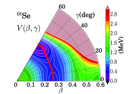
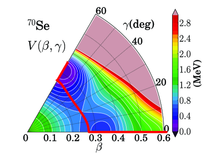
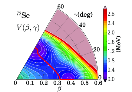
We show in Fig. 1 the collective potentials $V(\beta,\gamma)$ calculated for ^68,70,72Se. It is seen that two local minima always appear both at the oblate ($\gamma=60^{\circ}$) and prolate ($\gamma=0^{\circ}$) shapes, and, in all these nuclei, the oblate minimum is lower than the prolate minimum. The energy difference between them is, however, only several hundred keV and the potential barrier is low in the direction of triaxial shape (with respect to $\gamma$) indicating $\gamma$-soft character of these nuclei. In Fig. 1 we also show the collective paths (connecting the oblate and prolate minima) determined by using the 1D version of the ASCC method Hinohara et al. (2009). It is seen that they always run through the triaxial valley and never go through the spherical shape.

Figure 2: (Color online) Monopole- and quadrupole-pairing gaps for neutrons of ⁶⁸Se are plotted in the $(\beta,\gamma)$ deformation plane. (upper left) Monopole pairing gap $\Delta_{0}^{(n)}$. (lower left) Quadrupole pairing gap $\Delta_{20}^{(n)}$. (lower right) Quadrupole pairing gap $\Delta_{22}^{(n)}$. See Ref. Hinohara et al. (2008) for definitions of $\Delta_{0}^{(n)},\Delta_{20}^{(n)}$, and $\Delta_{22}^{(n)}$.

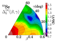
In Fig. 2, the monopole- and quadrupole-pairing gaps calculated for ⁶⁸Se are displayed. They show a significant $(\beta,\gamma)$ dependence. Broadly speaking, the monopole pairing decreases while the quadrupole pairing increases as $\beta$ increases.

III.3 Properties of the LQRPA modes

Figure 3: Frequencies squared $\omega^{2}$ of the LQRPA modes calculated for ⁶⁸Se are plotted as functions of $\beta$ or $\gamma$. The LQRPA modes adopted for calculation of the vibrational masses are connected with solid lines. (top) Dependence on $\gamma$ at $\beta=0.3$. (middle) Dependence on $\beta$ along the $\gamma=0.5^{\circ}$ line. (bottom) Dependence on $\beta$ along the $\gamma=30.5^{\circ}$ line.

In Fig. 3 the frequencies squared, $\omega_{i}^{2}(\beta,\gamma)$, of various LQRPA modes calculated for ⁶⁸Se are plotted as functions of $\beta$ and $\gamma$. In the region of the $(\beta,\gamma)$ plane where the collective potential energy is less than about 5 MeV, we can easily identify two collective modes among many LQRPA modes, whose $\omega_{i}^{2}(\beta,\gamma)$ are much lower than those of other modes. Therefore we adopt the two lowest frequency modes to derive the collective Hamiltonian. This result of numerical calculation supports our assumption that there exists a 2D hypersurface associated with large-amplitude quadrupole shape vibrations, which is approximately decoupled from other degrees of freedom. The situation changes when the collective potential energy exceeds about 5 MeV and/or the monopole-pairing gap becomes small. A typical example is presented in the bottom panel of Fig. 3. It becomes hard to identify two collective modes well-separated from other modes when $\beta>0.4$, where the collective potential energy is high (see Fig. 1) and the monopole-pairing gap becomes small (see Fig. 2). In this example, the second-lowest LQRPA mode in the $0.4<\beta<0.5$ region has pairing-vibrational character but becomes non-collective for $\beta>0.5$. In fact, many non-collective two-quasiparticle modes appear in its neighborhood. This region in the $(\beta,\gamma)$ plane is not important, however, because only tails of the collective wave function enter into this region.

Figure 4: Dependence on $\beta$ and $\gamma$ of the vibrational part of the metric $W(\beta,\gamma)$ calculated for ⁶⁸Se. (top) Dependence on $\gamma$ at $\beta=0.3$. (middle) Dependence on $\beta$ along the $\gamma=0.5^{\circ}$ line. (bottom) Dependence on $\beta$ along the $\gamma=30.5^{\circ}$ line. The cross symbols indicate values of the vibrational metric calculated for various choices of two LQRPA modes from among the lowest 40 LQRPA modes; the lowest mode is always chosen and the other is from the remaining 39 modes. The smallest vibrational metric is shown by solid line. For reference, the vibrational metric calculated using the IB vibrational mass is indicated by broken lines.

It may be useful to set up a prescription that works even in a difficult situation where it is not apparent how to choose two collective LQRPA modes. We find that the following prescription always works well for selecting two collective modes among many LQRPA modes. This may be called a minimal metric criterion. At each point on the $(\beta,\gamma)$ plane, we evaluate the vibrational part of the metric $W(\beta,\gamma)$ given by Eq. (44) for all combinations of two LQRPA modes, and find the pair that gives the minimum value. We show in Fig. 4 how this prescription actually works. In this figure, the $W(\beta,\gamma)$ values are plotted as functions of $\beta$ and $\gamma$ for many pairs of the LQRPA modes. In the situations where the two lowest-frequency LQRPA modes are well separated from other modes, this prescription gives the same results as choosing the two lowest-frequency modes (see the top and middle panels). On the other hand, a pair of the LQRPA modes different from the lowest two modes is chosen by this prescription in the region mentioned above (the bottom panel). This choice may be better than that using the lowest-frequency criterion, because we often find that a normal mode of pairing vibrational character becomes the second lowest LQRPA mode when the monopole-pairing gap significantly decreases in the region of large $\beta$. The small values of the vibrational metric implies that the direction of the infinitesimal displacement associated with the pair of the LQRPA modes has a large projection onto the ($\beta,\gamma$) plane. Therefore, this prescription may be well suited to our purpose of deriving the collective Hamiltonian for the $(\beta,\gamma)$ variables. It remains as an interesting open question for future to examine whether or not the explicit inclusion of the pairing vibrational degree of freedom as another collective variable will give us a better description in such situations.

III.4 Vibrational masses

Figure 5: (Color online) Vibrational masses, $D_{\beta\beta}(\beta,\gamma)$, $D_{\beta\gamma}(\beta,\gamma)/\beta$, and $D_{\gamma\gamma}(\beta,\gamma)/\beta^{2}$, in unit of MeV^-1 calculated for ⁶⁸Se.

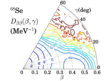
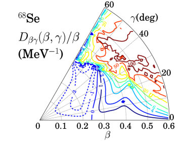
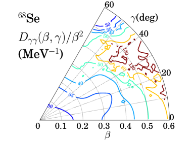
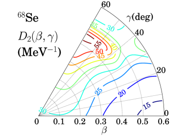
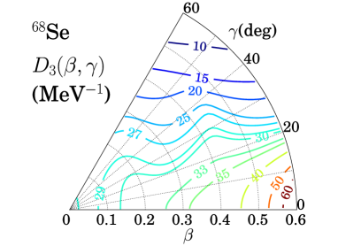
In Fig. 5 the vibrational masses calculated for ⁶⁸Se are displayed. We see that their values exhibit a significant variation in the $(\beta,\gamma)$ plane. In particular, the increase in the large $\beta$ region is remarkable.

Figure 6: (Color online) Ratios of the LQRPA vibrational masses to the IB vibrational masses, $D_{\beta\beta}/D^{({\rm IB})}_{\beta\beta}$ and $D_{\gamma\gamma}/D^{({\rm IB})}_{\gamma\gamma}$, calculated for ⁶⁸Se.

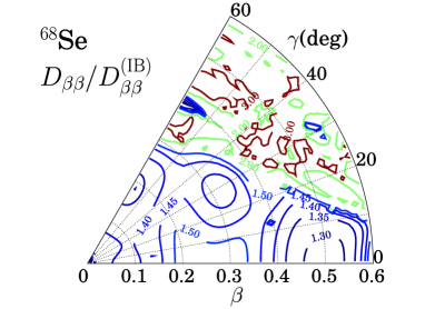
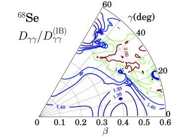
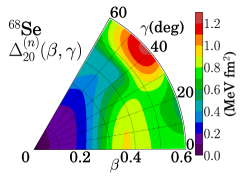
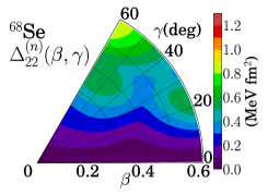
Figure 6 shows how the ratios of the LQRPA vibrational masses to the IB vibrational masses vary on the $(\beta,\gamma)$ plane. It is clearly seen that the LQRPA vibrational masses are considerably larger than the IB vibrational masses and their ratios change depending on $\beta$ and $\gamma$. In this calculation, the IB vibrational masses are evaluated using the well-known formula:

$$D^{(\rm IB)}_{\xi_{i}\xi_{j}}(\beta,\gamma)=2\sum_{\mu\bar{\nu}}\frac{\left\langle\mu\bar{\nu}\right|\displaystyle\frac{\partial\hat{H}_{\rm CHB}}{\partial\xi_{i}}\left|0\right\rangle\left\langle 0\right|\displaystyle\frac{\partial\hat{H}_{\rm CHB}}{\partial\xi_{j}}\left|\mu\bar{\nu}\right\rangle}{[E_{\mu}(\beta,\gamma)+E_{\bar{\nu}}(\beta,\gamma)]^{3}},$$ (52)

$$(\xi_{i}=\beta~{}{\rm or}~{}\gamma)$$

where $E_{\mu}(\beta,\gamma)$, $\left|0\right\rangle$, and $\left|\mu\bar{\nu}\right\rangle$ denote the quasiparticle energy, the CHB state $\left|\phi(\beta,\gamma)\right\rangle$ and the two-quasiparticle state  $a^{\dagger}_{\mu}a^{\dagger}_{\bar{\nu}}\left|\phi(\beta,\gamma)\right\rangle$, respectively (see Ref. Hinohara et al. (2008) for the meaning of the indices $\mu$ and $\bar{\nu}$).

The vibrational masses calculated for ^70,72Se exhibit behaviors similar to those for ⁶⁸Se.

III.5 Rotational masses

Figure 7: (Color online) Rotational masses $D_{k}(\beta,\gamma)$ in unit of MeV^-1, calculated for ⁶⁸Se. See Eq. (39) for the relation with the rotational moments of inertia ${\cal J}_{k}(\beta,\gamma)$.

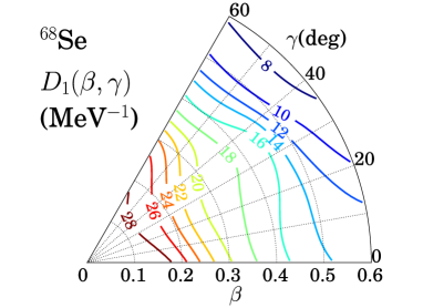
In Fig. 7, the LQRPA rotational masses $D_{k}(\beta,\gamma)$ calculated for ⁶⁸Se are displayed. Similarly to the vibrational masses discussed above, the LQRPA rotational masses also exhibit a remarkable variation over the $(\beta,\gamma)$ plane, indicating a significant deviation from the irrotational property.

Figure 8: (Color online) Ratios of the LQRPA rotational masses to the IB rotational masses, $D_{k}(\beta,\gamma)/D^{(\rm IB)}_{k}(\beta,\gamma)$, calculated for ⁶⁸Se.

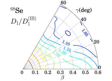
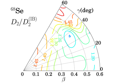
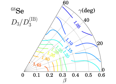
Figure 8 shows how the ratios of the LQRPA rotational masses $D_{k}(\beta,\gamma)$ to the IB cranking masses $D^{(\rm IB)}_{k}(\beta,\gamma)$ vary on the $(\beta,\gamma)$ plane. The rotational masses calculated for ^70,72Se exhibit behaviors similar to those for ⁶⁸Se.

As we have seen in Figs. 5–8, not only the vibrational and rotational masses but also their ratios to the IB cranking masses exhibit an intricate dependence on $\beta$ and $\gamma$. For instance, it is clearly seen that the ratios, $D_{k}(\beta,\gamma)/D^{(\rm IB)}_{k}(\beta,\gamma)$, gradually increase as $\beta$ decreases. This result is consistent with the calculation by Hamamoto and Nazarewicz Hamamoto and Nazarewicz (1994), where it is shown that the ratio of the Migdal term to the cranking term in the rotational moment of inertia (about the 1st axis) increases as $\beta$ decreases. Needless to say, the Migdal term (also called the Thouless-Valation correction) corresponds to the time-odd mean-field contribution taken into account in the LQRPA rotational masses, so that the result of Ref. Hamamoto and Nazarewicz (1994) implies that the ratio $D_{1}(\beta,\gamma)/D^{(\rm IB)}_{1}(\beta,\gamma)$, increases as $\beta$ decreases, in agreement with our result. To understand this behavior, it is important to note that, in the present calculation, the dynamical effect of the time-odd mean-field on $D_{1}(\beta,\gamma)$ is associated with the $K=1$ component of the quadrupole-pairing interaction and it always works and increase the rotational masses, in contrast to the behavior of the static quantities like the magnitude of the quadrupole-pairing gaps, $\Delta_{20}$ and $\Delta_{22}$, which diminish in the spherical shape limit. Obviously, this qualitative feature holds true irrespective of details of our choice of the monopole and quadrupole pairing interaction strengths.

The above results of calculation obviously indicate the need to take into account the time-odd contributions to the vibrational and rotational masses by going beyond the IB cranking approximation. In Refs. Li et al. (2009); Nikšić et al. (2007, 2009); Li et al. (2010), a phenomenological prescription is adopted to remedy the shortcoming of the IB cranking masses; that is, a constant factor in the range 1.40-1.45 is multiplied to the IB rotational masses. This prescription is, however, insufficient in the following points. First, the scaling only of the rotational masses (leaving the vibrational masses aside) violates the symmetry requirement for the 5D collective quadrupole Hamiltonian Bohr and Mottelson (1998); Belyaev (1965); Kumar and Baranger (1967) (a similar comment is made in Ref. Próchniak and Rohoziński (2009)). Second, the ratios take different values for different LQRPA collective masses ($D_{\beta\beta},D_{\beta\gamma},D_{\gamma\gamma},D_{1},D_{2}$, and $D_{3}$). Third, for every collective mass, the ratio exhibits an intricate dependence on $\beta$ and $\gamma$. Thus, it may be quite insufficient to simulate the time-odd mean-field contributions to the collective masses by scaling the IB cranking masses with a common multiplicative factor.

III.6 Check of self-consistency along the collective path

As discussed in Sec. II, the CHB+LQRPA method is a practical approximation to the ASCC method. It is certainly desirable to examine the accuracy of this approximation by carrying out a fully self-consistent calculation. Although, at the present time, such a calculation is too demanding to carry out for a whole region of the $(\beta,\gamma)$ plane, we can check the accuracy at least along the 1D collective path. This is because the 1D collective path is determined by carrying out a fully self-consistent ASCC calculation for a single set of collective coordinate and momentum. The 1D collective paths projected onto the $(\beta,\gamma)$ plane are displayed in Fig. 1. Let us use a notation $\left|\phi(q)\right\rangle$ for the moving-frame HB state obtained by self-consistently solving the ASCC equations for a single collective coordinate $q$ Hinohara et al. (2008, 2009). To distinguish from it, we write the CHB state as $\left|\phi(\beta(q),\gamma(q))\right\rangle$. This notation means that the values of $\beta$ and $\gamma$ are specified by the collective coordinate $q$ along the collective path. In other words, $\left|\phi(\beta(q),\gamma(q))\right\rangle$ has the same expectation values of the quadrupole operator as those of $\left|\phi(q)\right\rangle$. It is important to note, however, that they are different from each other, because $\left|\phi(\beta(q),\gamma(q))\right\rangle$ is a solution of the CHB equation which is an approximation of the moving-frame HB equation. Let us evaluate various physical quantities using the two state vectors and compare the results.

Figure 9: (Color online) Comparison of physical quantities evaluated with the CHB + LQRPA approximation and those with the ASCC method. Both calculations are carried out along the 1D collective path for ⁶⁸Se and the results are plotted as function of $\gamma(q)$. From the top to the bottom: 1) the collective potential, 2) monopole-pairing gaps, $\Delta_{0}^{(n))}$ and $\Delta_{0}^{(p)}$, for neutrons and protons, 3) frequencies squared $\omega^{2}$ of the lowest and the second-lowest modes obtained by solving the moving-frame QRPA and the LQRPA equations, 4) vibrational masses, $D_{\beta\beta}$, $D_{\beta\gamma}/\beta$, and $D_{\gamma\gamma}/\beta^{2}$, 5) rotational masses $D_{k}$. In almost all cases, results of the two calculations are indistinguishable, because they agree within the widths of the line.

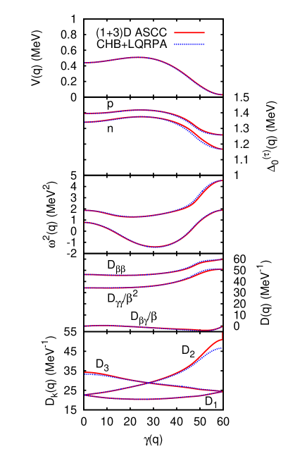
In Fig. 9 various physical quantities (the pairing gaps, the collective potential, the frequencies of the local normal modes, the rotational masses, and vibrational masses) calculated using the moving-frame HB state $\left|\phi(q)\right\rangle$ and the CHB state $\left|\phi(\beta(q),\gamma(q))\right\rangle$ are presented and compared. These calculations are carried out along the 1D collective path for ⁶⁸Se. Apparently, the results of the two calculations are indistinguishable in almost all cases, because they agree within the widths of the line. This good agreement implies that the CHB+LQRPA is an excellent approximation to the ASCC method along the collective path on the $(\beta,\gamma)$ plane. As we shall see in the next section, collective wave functions distribute around the collective path. Therefore, it may be reasonable to expect that the CHB+LQRPA method is a good approximation to the ASCC method and suited, at least, for describing the oblate-prolate shape mixing dynamics in ^68,70,72Se.

IV Large-amplitude shape-mixing properties of ^68,70,72Se

We have calculated collective wave functions solving the collective Schrödinger equation (40) and evaluated excitation spectra, quadrupole transition probabilities, and spectroscopic quadrupole moments. The results for low-lying states in ^68,70,72Se are presented in Figs. 10–15.

Figure 10: Excitation spectra and $B(E2)$ values calculated for ⁶⁸Se by means of the CHB+LQRPA method (denoted CHB+LQRPA) and experimental data Fischer et al. (2003, 2000); Obertelli et al. (2009). For comparison, results calculated using the IB cranking masses (denoted CHB+IB) and those obtained using the (1+3)D version of the ASCC method (denoted (1+3)D ASCC) are also shown. Only $B(E2)$’s larger than 1 Weisskopf unit (in the (1+3)D ASCC and/or the CHB+LQRPA calculations) are shown in units of $e^{2}$fm⁴.

Figure 11: (Color online) Vibrational wave functions squared $\beta^{4}|\Phi_{Ik}(\beta,\gamma)|^{2}$ calculated for ⁶⁸Se.

Figure 12: Same as Fig. 10 but for ⁷⁰Se. Experimental data is taken from Refs. Ljungvall et al. (2008); Rainovski et al. (2002).

Figure 13: (Color online) Same as Fig. 11 but for ⁷⁰Se.

Figure 14: Same as Fig. 10 but for ⁷²Se. Experimental data is taken from Refs. Ljungvall et al. (2008); Palit et al. (2001).

Figure 15: (Color online) Same as Fig. 11 but for ⁷²Se.

Figure 16: Spectroscopic quadrupole moments for ^68,70,72Se. Values calculated with the LQRPA collective masses are shown with the triangles. For comparison, values calculated with the IB collective masses and those obtained with the (1+3)D version of the ASCC method are also shown with the squares and the circles, respectively. The filled symbols show the values for the yrast states, while the open symbols those for the yrare states.

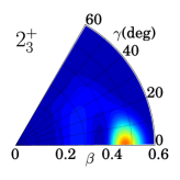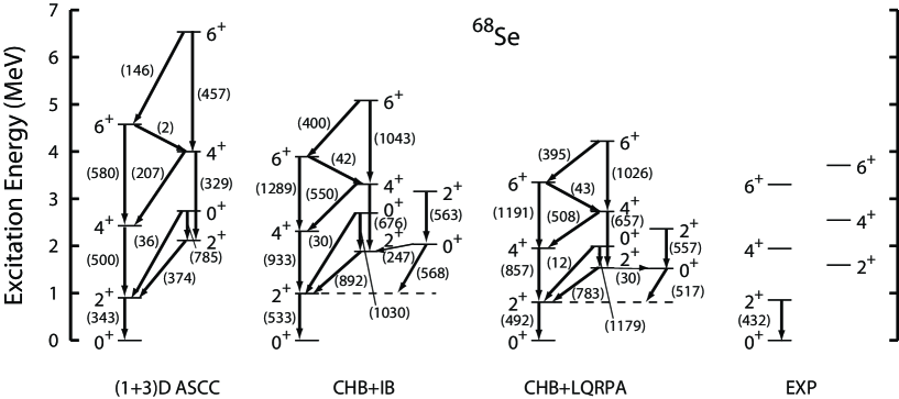
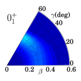
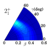
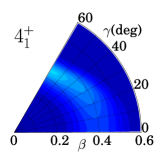
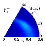
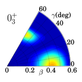
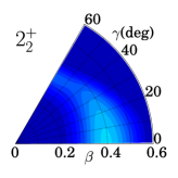
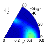
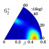
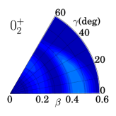
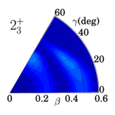
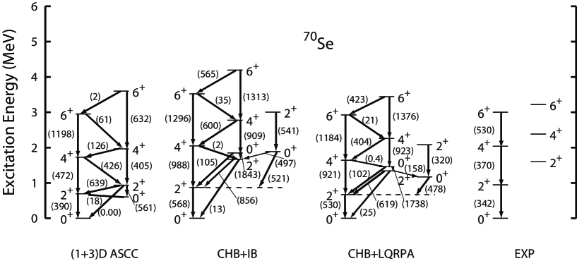
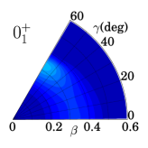
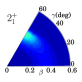
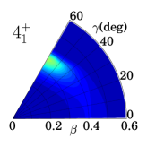
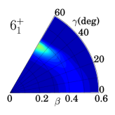
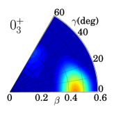
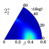
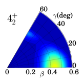
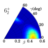
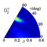
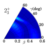
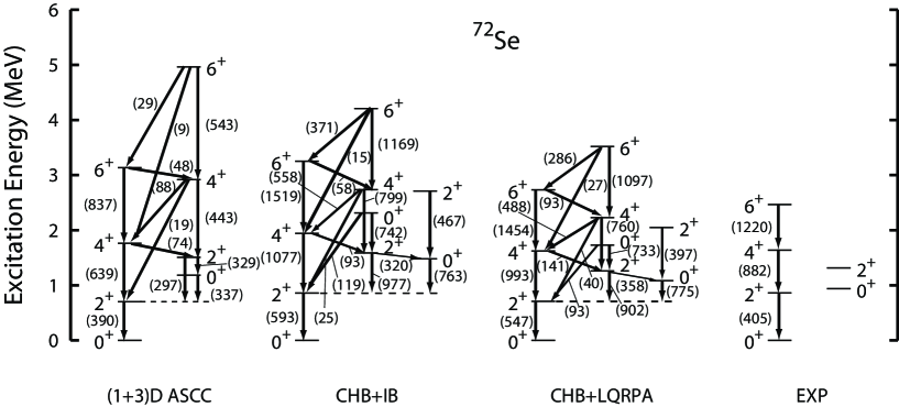
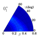
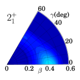
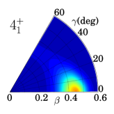
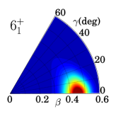
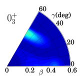
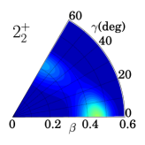
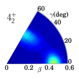
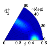
In Figs. 10, 12, and 14, excitation spectra and $B(E2)$ values for ⁶⁸Se, ⁷⁰Se, and ⁷²Se, calculated with the CHB+LQRPA method, are displayed together with experimental data. The eigenstates are labeled with $I^{\pi}=0^{+},2^{+},4^{+}$, and $6^{+}$. In these figures, results obtained using the IB cranking masses are also shown for the sake of comparison. Furthermore, the results calculated with the (1+3)D version of the ASCC method reported in our previous paper Hinohara et al. (2009) are shown also for comparison with the 5D calculations. We use the abbreviation (1+3)D to indicate that a single collective coordinate along the collective path describing large-amplitude vibration and three rotational angles associated with the rotational motion are taken into account in these calculations. The classification of the calculated low-lying states into families of two or three rotational bands is made according to the properties of their vibrational wave functions. These vibrational wave functions are displayed in Figs. 11, 13, and 15. In these figures, only the $\beta^{4}$ factor in the volume element (49) are multiplied to the vibrational wave functions squared leaving the $\sin 3\gamma$ factor aside. This is because all vibrational wave functions look like triaxial and the probability at the oblate and prolate shapes vanish if the $\sin 3\gamma$ factor is multiplied by them.

Let us first summarize the results of the CHB+LQRPA calculation. The most conspicuous feature of the low-lying states in these proton-rich Se isotopes is the dominance of the large-amplitude vibrational motion in the triaxial shape degree of freedom. In general, the vibrational wave function extends over the triaxial region between the oblate $(\gamma=60^{\circ}$) and the prolate ($\gamma=0^{\circ}$) shapes. In particular, this is the case for the $0^{+}$ states causing their peculiar behaviors; for instance, we obtain two excited $0^{+}$ states located slightly below or above the $2_{2}^{+}$ state. Relative positions between these excited states are quite sensitive to the interplay of large-amplitude $\gamma$-vibrational modes and the $\beta$-vibrational modes. This result of calculation is consistent with the available experimental data where the excited $0^{+}$ state has not yet been found, but more experimental data are needed to examine the validity of the theoretical prediction. Below, let us examine characteristic features of the theoretical spectra more closely for individual nuclei.

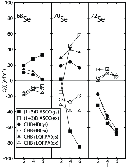
For ⁶⁸Se, we obtain the third band in low energy. The $0_{2}^{+}$ and $2^{+}_{3}$ states belonging to this band are also shown in Fig. 10. Their vibrational wave functions exhibit nodes in the $\beta$ direction (see Fig. 11) indicating that a $\beta$-vibrational mode is excited on top of the large-amplitude $\gamma$ vibrations. As a matter of course, this kind of state is outside of the scope of the (1+3)D calculation. The vibrational wave functions of the yrast $2_{1}^{+}$ and $4_{1}^{+}$ states exhibit localization in a region around the oblate shape, while the yrare $2_{2}^{+},4_{2}^{+}$, and $6_{2}^{+}$ states localize around the prolate shape. It is apparent, however, that all the wave functions significantly extend from $\gamma=0^{\circ}$ to $60^{\circ}$ over the triaxial region, indicating $\gamma$-soft character of these states. In particular, the yrare $4_{2}^{+}$ and $6_{2}^{+}$ wave functions exhibit two-peak structure consisting of the prolate and oblate peaks. The peaks of the vibrational wave function gradually shift toward a region of larger $\beta$ as the angular momentum increases. This is a centrifugal effect decreasing the rotational energy by increasing the moment of inertia. In the (1+3)D calculation, this effect is absent because the collective path is fixed at the ground state. Thus, the 5D calculation yields, for example, a much larger value for $B(E2;6_{1}^{+}\rightarrow 4_{1}^{+})$ in comparison with the (1+3)D calculation. Actually, in the 5D CHB+LQRPA calculation, the wave function of the yrast $6_{1}^{+}$ state localizes in the triaxial region (see Fig. 11) where the moment of inertia takes a maximum value. This leads to a small value for the spectroscopic quadrupole moment (see Fig. 16) because of the cancellation between the contributions from the oblate-like and prolate-like regions. This cancellation mechanism due to the large-amplitude $\gamma$ fluctuation is effective also in other states; although the spectroscopic quadrupole moments of the yrast $2_{1}^{+}$ and $4_{1}^{+}$ (yrare $2_{2}^{+},4_{2}^{+}$, and $6_{2}^{+}$) states are positive (negative) indicating their oblate-like (prolate-like) character, their absolute magnitudes are rather small.

The $E2$-transition probabilities exhibit a pattern reminiscent of the $\gamma$-unstable situation; for instance, $B(E2;6_{2}^{+}\to 6_{1}^{+})$, $B(E2;4_{2}^{+}\to 4_{1}^{+})$, and $B(E2;2_{2}^{+}\to 2_{1}^{+})$ are much larger than $B(E2;6_{2}^{+}\to 4_{1}^{+})$, $B(E2;4_{2}^{+}\to 2_{1}^{+})$, and $B(E2;2_{2}^{+}\to 0_{1}^{+})$; see Fig. 10. Thus, the low-lying states in ⁶⁸Se may be characterized as an intermediate situation between the oblate-prolate shape coexistence and the Wilets-Jean $\gamma$-unstable model Wilets and Jean (1956). Using the phenomenological Bohr-Mottelson collective Hamiltonian, we have shown in Ref. Sato et al. (2010) that it is possible to describe the oblate-prolate shape coexistence and the $\gamma$-unstable situation in a unified way varying a few parameters controlling the degree of oblate-prolate asymmetry in the collective potential and the collective masses. The two-peak structure seen in the $4_{2}^{+}$ and $6_{2}^{+}$ states may be considered as one of the characteristics of the intermediate situation. It thus appears that the excitation spectrum for ⁶⁸Se (Fig. 10) serves as a typical example of the transitional phenomena from the $\gamma$-unstable to the oblate-prolate shape coexistence situations.

Let us make a comparison between the spectra in Fig. 10 obtained with the LQRPA collective masses and that with the IB cranking masses. It is obvious that the excitation energies are appreciably overestimated in the latter. This result is as expected from the too low values of the IB cranking masses. The result of our calculation is in qualitative agreement with the HFB-based configuration-mixing calculation reported by Ljungvall et al. Ljungvall et al. (2008) in that both calculations indicate the oblate (prolate) dominance for the yrast (yrare) band in ⁶⁸Se. Quite recently, the $B(E2;2_{1}^{+}\to 0_{1}^{+})$ value has been measured in experiment Obertelli et al. (2009). The calculated value (492 $e^{2}$fm⁴) is in fair agreement with the experimental data (432 $e^{2}$fm⁴).

The result of calculation for ⁷⁰Se (Figs. 12 and 13) is similar to that for ⁶⁸Se. The vibrational wave functions of the yrast $2_{1}^{+},4_{1}^{+}$, and $6_{1}^{+}$ states localize in a region around the oblate shape, exhibiting, at the same time, long tails in the triaxial direction. We note here that, differently from the ⁶⁸Se case, the $6_{1}^{+}$ wave function keeps the oblate-like structure. On the other hand, the yrare $2_{2}^{+},4_{2}^{+}$, and $6_{2}^{+}$ states localize around the prolate shape, exhibiting, at the same time, small secondary bumps around the oblate shape. For the yrare $2_{2}^{+}$ state, we obtain a strong oblate-prolate shape mixing in the (1+3)D calculation Hinohara et al. (2009). This mixing becomes weaker in the present 5D calculation, resulting in the reduction of the $B(E2;4_{1}^{+}\to 2_{2}^{+})$ value. Similarly to ⁶⁸Se, we obtain two excited $0^{+}$ states in low energy. We see considerable oblate-prolate shape mixings in their vibrational wave functions, but, somewhat differently from those in ⁶⁸Se, the second and third $0^{+}$ states in ⁷⁰Se exhibit clear peaks at the oblate and prolate shapes, respectively, Their energy ordering is quite sensitive to the interplay of the large-amplitude $\gamma$ vibration and the $\beta$ vibrational modes. The calculated spectrum for ⁷⁰Se is in fair agreement with the recent experimental data Rainovski et al. (2002) , although the $B(E2)$ values between the yrast states are overestimated.

The result of calculation for ⁷²Se (Figs. 14 and 15) presents a feature somewhat different from those for ⁶⁸Se and ⁷⁰Se; that is, the yrast $2_{1}^{+},4_{1}^{+}$, and $6_{1}^{+}$ states localize around the prolate shape instead of the oblate shape. The localization develops with increasing angular momentum. On the other hand, similarly to the ^68,70Se cases, the yrare $2_{2}^{+},4_{2}^{+}$, and $6_{2}^{+}$ states exhibit the two-peak structure. The spectroscopic quadrupole moments of the $2_{1}^{+},4_{1}^{+}$, and $6_{1}^{+}$ states are negative, and their absolute magnitude increases with increasing angular momentum (see Fig. 16) reflecting the developing prolate character in the yrast band, while those of the yrare states are small because of the two-peak structure of their vibrational wave functions, that is, due to the cancellation of the contributions from the prolate-like and oblate-like regions. Also for ⁷²Se, we obtain two excited $0^{+}$ states in low energy, but they show features somewhat different from the corresponding excited $0^{+}$ states in ^68,70Se. Specifically, the vibrational wave functions of the second and third $0^{+}$ states exhibit peaks at the prolate and oblate shape, respectively. As seen in Fig. 14, our results of calculation for the excitation energies and $B(E2)$ values are in good agreement with the recent experimental data Ljungvall et al. (2008) for the yrast $2_{1}^{+},4_{1}^{+}$, and $6_{1}^{+}$ states in ⁷²Se. Experimental $E2$-transition data are awaited for understanding the nature of the observed excited band.

V Conclusions

On the basis of the ASCC method, we have developed a practical microscopic approach, called CHFB+LQRPA, of deriving the 5D quadrupole collective Hamiltonian and confirmed its efficiency by applying it to the oblate-prolate shape coexistence/mixing phenomena in proton-rich ^68,70,72Se. The results of numerical calculation for the excitation energies and $B(E2)$ values are in good agreement with the recent experimental data Obertelli et al. (2009); Ljungvall et al. (2008) for the yrast $2_{1}^{+},4_{1}^{+}$, and $6_{1}^{+}$ states in these nuclei. It is shown that the time-odd components of the moving mean-field significantly increase the vibrational and rotational collective masses and make the theoretical spectra in much better agreement with the experimental data than calculations using the IB cranking masses. Our analysis clearly indicates that low-lying states in these nuclei possess a transitional character between the oblate-prolate shape coexistence and the so-called $\gamma$ unstable situation where large-amplitude triaxial-shape fluctuations play a dominant role.

Finally, we would like to list a few issues for the future that seems particularly interesting. First, fully self-consistent solution of the ASCC equations for determining the two-dimensional collective hypersurface and examination of the validity of the approximations adopted in this paper in the derivation of the CHFB+LQRPA scheme. Second, application to various kind of collective spectra associated with large-amplitude collective motions near the yrast lines (as listed in Ref. Matsuyanagi et al. (2010)). Third, possible extension of the quadrupole collective Hamiltonian by explicitly treating the pairing vibrational degrees of freedom as additional collective coordinates. Fourth, use of the Skyrme energy functionals + density-dependent contact pairing interaction in place of the P+Q force, and then modern density functionals currently under active development. Fifth, application of the CHFB+LQRPA scheme to fission dynamics. The LQRPA approach enables us to evaluate, without need of numerical derivatives, the collective inertia masses including the time-odd mean-field effects.