*0pt plain latex[] [0][][]0

NON-GAUSSIANITY AND STATISTICAL
ANISOTROPY IN COSMOLOGICAL
INFLATIONARY MODELS

by

CÉSAR ALONSO VALENZUELA TOLEDO
Physicist, MSc

Grupo de Investigación en Relatividad y Gravitación
Escuela de Física, Universidad Industrial de Santander
Ciudad Universitaria, Bucaramanga, Colombia
Grupo de física-fenomenología de partículas elementales y cosmología Centro de Investigaciones, Universidad Antonio Nariño
Cra 3 Este # 47A-15, Bogotá D.C., Colombia.  

NON-GAUSSIANITY AND STATISTICAL
ANISOTROPY IN COSMOLOGICAL
INFLATIONARY MODELS
CÉSAR ALONSO VALENZUELA TOLEDO
Physicist, MSc Thesis directed by
Dr. YEINZON RODRÍGUEZ GARCÍA A thesis submmited in partial fulfillment of the requirements for the degree of Doctor in Sciences – Physics
 

To Juan Camilo, César David and María Sofía.

TÍTULO : NO GUSSIANIDAD Y ANISOTROPÍA ESTADÍSTICA EN MODELOS COSMOLÓGICOS INFLACIONARIOS .

AUTOR : VALENZUELA TOLEDO, César Alonso .

PALABRAS CLAVES: Cosmología, No gaussianidad, Inflación, Anisotropía estadistíca, Teoría de perturbaciones cosmológicas, Perturbación primordial en la curvatura.

DESCRIPCIÓN: Se estudian los descriptores estadísticos para algunos modelos cosmológicos inflacionarios que permiten obtener altos niveles de no gaussianidad y violacion de la isotropía estadística. Básicamente, se estudian dos tipos de modelos: modelos que involucran sólo campos escalares, particularmente un modelo inflacionario de rodadura lenta con potencial escalar cuadrático de dos componentes con términos cinéticos canónicos, y modelos que incluyen campos escalares y vectoriales.

Se muestra que para el modelo de rodadura lenta con potencial escalar cuadrático de dos componentes, es possible obtener valores altos y observables para los niveles de no gaussianidad $f_{NL}$ y $\tau_{\rm NL}$ en el bi-espectro $B_{\zeta}$ y en el tri-espectro $T_{\zeta}$, respectivamente, de la perturbación primordial en la curvatura $\zeta$. Se consideran contribuciones a nivel árbol y a un lazo en el espectro $P_{\zeta}$, en el bi-espectro $B_{\zeta}$ y en el tri-espectro $T_{\zeta}$. Se muestra que valores considerables se pueden obtener aun cuando $\zeta$ es generada durante inflación. Cinco aspectos son considerados cuando se extrae el espacio disponible de parámetros: 1. El asegurar la existencia de un régimen perturbativo de tal manera que la expansión en serie de $\zeta$, y su truncamiento, sean válidas. 2. El determinar las condiciones correctas que determinan el peso relativo de las correcciones a nivel árbol y a un lazo. 3. El satisfacer la condición de normalización de espectro. 4. El cumplir la restricción observacional del índice espectral. 5. El asegurar un monto de inflación mínimo necesario para resolver el problema de horizonte.

Para los modelos que incluyen campos escalares y vectoriales, nuevamente se estudia el espectro $P_{\zeta}$, el bi- espectro $B_{\zeta}$ y el tri-espectro $T_{\zeta}$ de la perturbación primordial en la curvatura, cuando $B_{\zeta}$ y $T_{\zeta}$ son generados por perturbaciones escalares y vectoriales. Se estudian las contribuciones a nivel árbol y a un lazo, considerando que las ultimas puedan dominar sobre las primeras. Se calculan los niveles de no gaussianidad $f_{NL}$ y $\tau_{\rm NL}$, y se encuentran relaciones de consistencia entre éstos y el nivel de anisotropía estadística $g_{\zeta}$ en el espectro $P_{\zeta}$, concluyendo que para valores pequeños de $g_{\zeta}$ los niveles de no-gaussianidad pueden ser altos, en algunos casos excediendo las cotas observacionales actuales.

TITLE: NON-GAUSSIANITY AND STATISTICAL ANISOTROPY IN COSMOLOGICAL INFLATIONARY MODELS .

AUTHOR: VALENZUELA TOLEDO, César Alonso .

KEY WORDS: Cosmology, Non-gaussianity, Inflation, Statistical anisotropy, Cosmological perturbation theory, Primordial curvature perturbation.

DESCRIPTION: We study the statistical descriptors for some cosmological inflationary models that allow us to get large levels of non-gaussianity and violations of statistical isotropy. Basically, we study two different class of models: a model that include only scalar field perturbations, specifically a subclass of small-field slow-roll models of inflation with canonical kinetic terms, and models that admit both vector and scalar field perturbations.

We study the former to show that it is possible to attain very high, including observable, values for the levels of non-gaussianity $f_{NL}$ and $\tau_{\rm NL}$ in the bispectrum $B_{\zeta}$ and trispectrum $T_{\zeta}$ of the primordial curvature perturbation $\zeta$ respectively. Such a result is obtained by taking care of loop corrections in the spectrum $P_{\zeta}$, the bispectrum $B_{\zeta}$ and the trispectrum $T_{\zeta}$. Sizeable values for $f_{NL}$ and $\tau_{\rm NL}$ arise even if $\zeta$ is generated during inflation. Five issues are considered when constraining the available parameter space: 1. we must ensure that we are in a perturbative regime so that the $\zeta$ series expansion, and its truncation, are valid. 2. we must apply the correct condition for the (possible) loop dominance in $B_{\zeta}$ and/or $P_{\zeta}$. 3. we must satisfy the spectrum normalisation condition. 4. we must satisfy the spectral tilt constraint. 5. we must have enough inflation to solve the horizon problem.

For the latter we study the spectrum ${\cal P}_{\zeta}$, bispectrum $B_{\zeta}$ and trispectrum of the primordial curvature perturbation when $\zeta$ is generated by scalar and vector field perturbations. The tree-level and one-loop contributions from vector field perturbations are worked out considering the possibility that the one-loop contributions may be dominant over the tree level terms. The levels of non-gaussianity $f_{NL}$ and $\tau_{\rm NL}$, are calculated and related to the level of statistical anisotropy in the power spectrum, $g_{\zeta}$. For very small amounts of statistical anisotropy in the power spectrum, the levels of non-gaussianity may be very high, in some cases exceeding the current observational limit.

Chapter 1          INTRODUCTION

The corner-stone of modern cosmology is that, at least on large scales, the visible universe seems to be the same in all directions around us and around all points, i.e. the Universe is almost homogeneous and isotropic. This is borne out by a variety of observations, particulary observations of cosmic microwave background (CMB); this radiation has been traveling to us for about 14000 million years (see Fig. 1.1), supporting the conclusion that the Universe at sufficiently large distances is nearly the same. On the other hand, it is apparent that nearby regions of the observable Universe are at present highly inhomogeneous, with material clumped into stars, galaxies and galaxy clusters. It is believed that these structures have formed over the time via gravitational attraction, from a distribution that was more homogeneous in the past.

The large-scale behavior of the Universe can be described by assuming a homogeneous background. On this background, we can superimpose the short scale irregularities. For much of the evolution of the observable Universe, these irregularities can be considered to be small perturbations on the evolution of the background (unperturbed) Universe. The metric of unperturbed Universe is called the Friedman-Leimatre-Roberson-Walker metric, and its line element can be to written as:

$$ds^{2}=-dt^{2}+a^{2}(t)\left(dr^{2}+r^{2}(d\theta^{2}+\sin\phi^{2}d\phi^{2}\right),$$ (1.1)

where $a(t)$ is the scale factor and $r,\theta,\phi$ are the spherical comoving coordinates

The model described by the above metric is known as the standard cosmological model (known also as Big-Bang cosmological model) [66, 171, 172, 173, 216] and is the successful framework that describes the observed properties of the Universe: homogeneity and isotropy at large scales, Hubble expansion, almost 14 billion years of evolution in agreement with globular clusters and radioactive isotopes dating, cosmic microwave background radiation (CMB) confirmed by Penzias and Wilson’s discovery in 1965 [48, 164], and the relative abundances of light elements [9, 10, 67, 93, 161, 215, 217] in full agreement with observation.

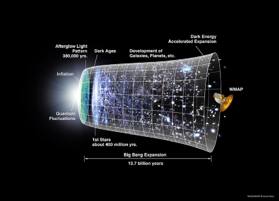
Figure 1.1: A representation of the evolution of the universe over 13.7 billion years. The far left depicts the earliest moment we can now probe, when a period of “ inflation ” produced a burst of exponential growth in the universe. (Size is depicted by the vertical extent of the grid in this graphic.) For the next several billion years, the expansion of the universe gradually slowed down as the matter in the universe pulled on itself via gravity. More recently, the expansion has begun to speed up again as the repulsive effects of dark energy have come to dominate the expansion of the universe. The afterglow light seen by WMAP was emitted about 380,000 years after inflation and has traversed the universe largely unimpeded since then. The conditions of earlier times are imprinted on this light; it also forms a backlight for later developments of the universe (Courtesy of the NASA/WMAP Science Team [159]).

The introduction of a period of exponential expansion (called inflationary) [8, 82, 131], prior to the Big-Bang, brought an elegant solution to the horizon, flatness, and unwanted relics problems that were present in the original standard cosmological model [8, 82, 117, 131, 169]. In spite of its success at solving the above mentioned problems, the inflationary period became perhaps more important because of its ability to stretch the quantum fluctuations of the fields living in the FRW spacetime [18, 83, 87, 131, 154, 156, 169, 201], making them classical [7, 36, 78, 84, 110, 133, 136, 140, 144, 150, 160] and almost constant soon after horizon exit. They correspond to small inhomogeneities in the energy density and are responsible, via gravitational attraction, of the large-scale structure seen today in the Universe. If this scenario turned to be correct, the energy density inhomogeneities should have left their trace in the CMB released at the time of recombination. Indeed, the Cosmic Background Explorer (COBE) in 1992 [158] found and mapped small anisotropies in the CMB temperature of the order of 1 part in $10^{5}$ (with average temperature $T_{0}=2.725\pm 0.002$ K [24]), on scales of order thousands of Megaparsecs. With 30 times better angular resolution and sensitivity than COBE, the Wilkinson Microwave Anisotropy Probe (WMAP) [159] confirmed this picture (see Fig. 1.2), measuring in turn the cosmological parameters with a $1\%$ order precision [119] on scales of order tens of Megaparsecs. The PLANCK satellite [59, 206], launched in may 2009, will be able to refine these observations (see Fig. 1.3 and 1.4). With 10 times better angular resolution and sensitivity than WMAP, PLANCK promises to determine the temperature anisotropies with a resolution of the order of 1 part in $10^{6}$, and the cosmological parameters with a $0.1\%$ order precision.

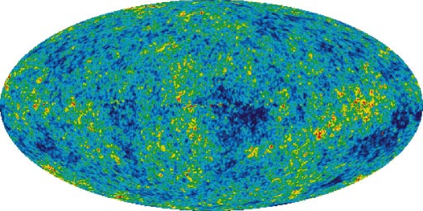
Figure 1.2: CMB temperature anisotropies as seen by the WMAP satellite (five years resuls) [119]. The oval shape is a projection to display the whole sky. The temperature anisotropies are found to be of the order of 1 part in $10^{5}$. The background temperature is $T_{0}=2.725\pm 0.002$ K; regions at that temperature are in very light blue. The hottest regions (in red) correspond to $\Delta T\simeq 200\mu{\rm K}$. The coldest regions (in very dark blue) correspond to $\Delta T\simeq-200\mu{\rm K}$ (Courtesy of the NASA/WMAP Science Team [159]).

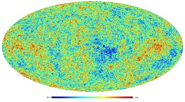
Figure 1.3: Simulation of the CMB temperature anisotropies as seen by the PLANCK satellite. PLANCK will provide a map of the CMB field at all angular resolutions greater than 10 arcminutes and with a temperature resolution of the order of 1 part in $10^{6}$ (ten times better than WMAP) (Courtesy of ESA’s PLANCK mission [59]).

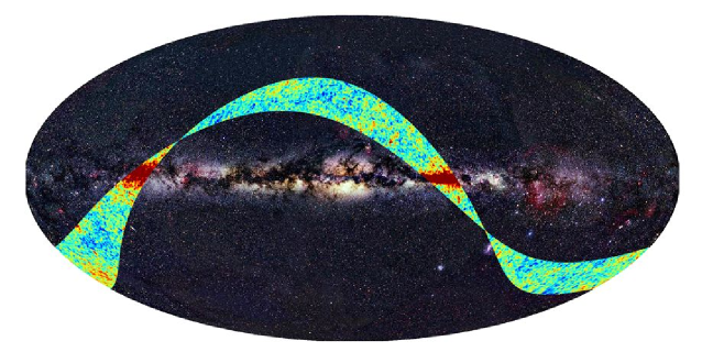
Figure 1.4: A map of the area of the sky mapped by PLANCK during the first light survey. The colours indicate the magnitude of the deviations of the temperature of the Cosmic Microwave Background from its average value (red is hotter and blue is colder). (Courtesy of ESA’s PLANCK mission [59]).

The anisotropies in the CMB temperature $\delta T/T_{0}$ are directly related to the perturbation in the spatial curvature $\zeta$ (Sachs-Wolfe effect), whose primarily origin is the stretched quantum fluctuations of one or several scalar fields $\phi_{i}$ that fill the Universe during inflation [140, 176]:

$$\left(\frac{\delta T}{T_{0}}\right)_{k}=-\frac{1}{5}\,\zeta_{k}\,.$$ (1.2)

The quantity $\zeta$ is related to the perturbation in the intrinsic curvature of space-time slices with uniform energy density [149]:

$${}^{(3)}R=\frac{4}{a^{2}}\;\nabla^{2}\psi\;,$$ (1.3)

where $\psi$ is the first order scalar perturbation in the spacial metric.

Astronomers work with the observable quantity $\delta T/T$ and theoretical cosmologists work with $\zeta$. Therefore, we may study the statistical porperties of the observed $\delta T/T$ through the spectral functions associated with the primordial curvature perturbation $\zeta$, whose properties are in general model dependent. Knowing the statistical descriptors of $\zeta$ for some particular and well motivated cosmological model proposed for the origin of large scale strucutre, we can reject the model or keep it, because some of the statistical descriptors for $\delta T/T$ are known with good acuracy or at least have an upper bound [119].

The statistical properties of the CMB temperature anisotropies can be then described in terms of the spectral functions, like the spectrum, bispectrum, trispectrum, etc., of the primordial curvature perturbation $\zeta$. This spectral functions are given in terms of other quantities, which have an observational value or an uppper bound. For example, the spectrum $P_{\zeta}$ is parametrized in terms of an amplitude ${{\cal P}_{\zeta}}^{1/2}$, a spectral index $n_{\zeta}$ and the level of statistical anisotropy $g_{\zeta}$; the bispectrum $B_{\zeta}$ and trispectrum $T_{\zeta}$ are parametrized in terms of products of the spectrum $P_{\zeta}$ and the quantities $f_{\rm NL}$, and $\tau_{\rm NL}$ and $g_{\rm NL}$, respectively. As we will see in the next chapter, the statistical descriptors $f_{\rm NL}$, $\tau_{\rm NL}$ and $g_{\rm NL}$ are usually called levels of non-gaussianity, because non zero values for these quantities imply non-gaussianity in the primordial curvature perturbation $\zeta$ as well in the constrast in the temperature of the CMB radiation $\delta T/T$. The non-gaussian characteristics in the CMB are actually present in the observation [119] as we will see in more detail in Section 2.4. The status of observation can be summarized as follows: the spectral amplitude ${{\cal P}_{\zeta}}^{1/2}=(4.957\pm 0.094)\times 10^{-5}$ [35], the spectral index $n_{\zeta}=0.960\pm 0.014$ at $2\sigma$ [119], the level of non-gaussianity $f_{\rm NL}$ in the bispectrum is in the range $-9<f_{NL}<111$ at $2\sigma$ [119]; and there is no observational bound on the levels of non-gaussinity $\tau_{\rm NL}$ and $g_{\rm NL}$ in the trispectrum $T_{\zeta}$. The amount of statistical anisotropy $g_{\zeta}$ in the spectrum $P_{\zeta}$ is in the range $g_{\zeta}\simeq 0.290\pm 0.093$ [79].

Regarding the statistical descriptors, non-gaussianity in the primordial curvature perturbation $\zeta$ is one of the subjects of more interest in modern cosmology, because the non-gaussianity parameters $f_{\rm NL}$ and $\tau_{\rm NL}$ together with the spectrum amplitude $A_{\zeta}$ and spectral index $n_{\zeta}$ allow us to discriminate between the different models proposed for the origin of the large-scale structure (see for example Refs. [3, 5, 6]). The most studied and popular models are those called the slow-roll models with canonical kinetic terms, because of their simplicity and because they easily satisfy the spectral index $n_{\zeta}$ requierements from observation. However, the usual predictions of these models is that the levels of non-gaussianity in the primordial curvature perturbation are expected to be unobservable [22, 148, 191, 211, 226]. However, as we will show in chapters 3 and 4, there are some aditional issues that have not been taken into account in the current literature. We study these issues to show that it is possible to generate sizeable and observable levels of non-gaussianity in a subclass of small- field slow-roll inflationary models with canonical kinetic terms; our main conclussion is that if non-gaussianity is detected, the aforementioned models could have strong possibilities to be the ones responsibles for the formation of the large-scale structure.

According to the usual assumption, one or more of these scalar field perturbations are responsible for the curvature perturbation. In that case, the $n$-point correlators of $\zeta$ are translationally and rotationally invariants. However, violations of such invariances entail modifications of the usual definitions for the spectral functions in terms of the statistical descriptors [1, 12, 41]. These violations may be consequences either of the presence of vector field perturbations [12, 19, 49, 50, 51, 52, 53, 54, 73, 74, 75, 76, 94, 95, 96, 97, 102, 103, 113, 224], spinor field perturbations [30, 194], or p-form perturbations [70, 71, 111, 115, 116], contributing significantly to $\zeta$, of anisotropic expansion [17, 30, 47, 81, 97, 102, 115, 165, 166, 218] or of an inhomogeneous background [12, 41, 52]. Violation of the statistical isotropy (i.e. violation of the rotational invariance in the $n$-point correlators of $\zeta$) seems to be present in the data [14, 80, 88, 178] and, although its statistical significance is still low, the continuous presence of anomalies in every CMB data analysis (see for instance Refs. [34, 58, 62, 63, 85, 86, 91, 92, 122, 123, 162, 184, 205]) suggests the evidence might be decisive in the forthcoming years. The presence of vector fields in the inflationary dynamics is not only important to be responsible of violations of the statistical isotropy, they also may generate sizeable levels of non-gaussianity described by $f_{\rm NL}$ and $\tau_{\rm NL}$; particularly we will show in Chapter 5, that including vector fields allows us to get consistency relations between the statistical descriptors, more precisely between the non-gaussianity levels $f_{\rm NL}$ and $\tau_{\rm NL}$ and the amount of statistical anisotropy $g_{\zeta}$.

Because of the progressive improvement in the accuracy of the satellite measurements described above, it is pertinent to study the statistical descriptors of the primordial curvature perturbation $\zeta$, for cosmological models of the origin of the large-scale structure in the Universe. It is very important because they could be a crucial tool to discriminate between some of most usual cosmological models [5, 6].

The layout of the thesis is the following: the Chapter 2 is devoted to study the statistical descriptors for a probability distribution function and its relation with the observational parameters, i.e., the spectrum amplitude, the spectral index the levels of non-gaussianity $f_{\rm NL}$ and $\tau_{\rm NL}$ in the bispectrum $B_{\zeta}$ and trispectrum $T_{\zeta}$ respectively and the level of statistical anisotropy in the power spectrum, $g_{\zeta}$. In this chapter, we also review some generalities of the $\delta N$ formalism, it has become the standard technique to calculate $\zeta$ and its statistical descriptors. In Chapters 3 and 4 we show that it is possible to attain very high, including observable, values for the levels of non-gaussianity $f_{NL}$ and $\tau_{\rm NL}$, in a subclass of small-field slow-roll models of inflation with canonical kinetic terms. Comparison with current observationally bounds is made. Chapter 5 is devoted to study the statistical descriptors of the primordial curvature perturbation $\zeta$ when scalar and vector fields perturbations are present in the inflationary dynamicc. The levels of non-gaussianity $f_{\rm NL}$ and $\tau_{\rm NL}$ are calculated and related to the level of statisitcal anisotropy in the power spectrum, $g_{\zeta}$. We show that the levels of non-gaussianity may be very high, in some cases exceeding the current observationally limit. Finally we conclude in Chapter 6.

Chapter 2          $\delta N$ FORMALISM AND STATISTICAL DESCRIPTORS FOR $\zeta$

 SECTION 2.1      Introduction

The primordial curvature perturbation $\zeta$, as well as the contrast in the temperature of the cosmic microwave background radiation $\delta T/T$ and the gravitational potential $\Phi_{g}$, are examples of cosmological functions of space and time being described by probability distribution functions. In particular, the probability distribution function $f(\zeta)$ for $\zeta$ has well defined statistical descriptors which depend directly upon the particular inflationary model and that are suitable for comparison with present observational data. Such a comparison allows us either to reject or to keep particular inflationary models as those which better represent nature’s behaviour. In this chapter we give a complete and general description of the $\delta N$ formalism including both scalar and vector fields. This formalism is a powerful tool and it is commonly used to calculate the primordial curvature perturbation $\zeta$. We also present a cosmologically motivated description of the statistical descriptors for probability distribution functions, focusing mainly on $f(\zeta)$. Finally, in Section 2.4 we give the observational constraints for $\zeta$.

 SECTION 2.2      The $\delta N$ formalism

The $\delta N$ formalism [52, 139, 142, 181, 182, 202] provides a powerful method for calculating $\zeta$ and all its statistical descriptors at any desired order in cosmological perturbation theory. The $\delta N$ formalism for scalar field perturbations was given at the linear level in Refs. [181, 202] and at the non-linear level, which generates non- gaussianity, it was described in Refs. [139, 142]. In a recent paper [52] the $\delta N$ formalism was extended to include vector as well as scalar fields. In this section, we give a brief review of the formalism without assuming statistical isotropy and define the primordial curvature perturbation $\zeta$.

In the cosmological standard model [155] the observable Universe is homogeneous and isotropic, being described by the unperturbed Friedmann-Robertson-Walker metric whose line element, for a spatially flat universe, looks as follows:

$$ds^{2}=-dt^{2}+a^{2}(t)\delta_{ij}dx^{i}dx^{j}\,,$$ (2.1)

where $a(t)$ is the global expansion parameter, $t$ is the cosmic time, and ${\bf x}$ represents the position in cartesian spatial coordinates. The homogeneity and isotropy conditions describe very well the Universe at large scales, but departures from the unperturbed background are observationally evident at smaller scales.

One way to parametrize the departures from the homogeneous and isotropic background is to include perturbations in the metric, for which we have to define a slicing and a threading. The slicing will be defined so that the energy density in fixed-$t$ slices of spacetime is uniform. The threading will correspond to comoving fixed-$x$ world lines. With generic coordinates the perturbed metric of the perturbed universe may be defined as

$$ds^{2}=g_{\mu\nu}dx^{\mu}dx^{\nu}\,.$$ (2.2)

To define the cosmological perturbations, one chooses a coordinate system in the perturbed universe, and then compares that universe with an unperturbed one. The unperturbed universe is taken to be homogeneous, and is usually taken to be isotropic as well.

2.2.1     The curvature perturbation

To define the curvature perturbation, we smooth the metric tensor and the energy-momentum tensor on a comoving scale $R$ and one considers the super-horizon regime $aR>H^{-1}$ where $H\equiv\dot{a}/a$ is the Hubble parameter and $a(t)$ is the scale factor normalised to 1 at present. The energy density $\rho$ and pressure $P$ are smoothed on the same scale. On the reasonable assumption that the smoothing scale is the biggest relevant scale, spatial gradients of the smoothed metric and energy-momentum tensors will be negligible. As a result, the evolution of these quantities at each comoving location will be that of some homogeneous ‘separate universe’. In contrast with earlier works on the separation universe assumption, we will in this section allow the possibility that the separate universes are anisotropic even though homogoneous.

We consider the slicing of spacetime with uniform energy density, and the threading which moves with the expansion (comoving threading). By virtue of the separate universe assumption, the threading will be orthogonal to the slicing. The spatial metric can then be written as

$$g_{ij}({\mathbf{x}},t)\equiv a^{2}(t)e^{2\zeta({\mathbf{x}},t)}\left(Ie^{2h({\mathbf{x}},t)}\right)_{ij},$$ (2.3)

where $I$ is the unit matrix, and the matrix $h$ is traceless so that $Ie^{2h}$ has unit determinant. The smoothing scale is chosen to be somewhat shorter than the scales of interest, so that the Fourier components of $\zeta$ on those scales is unaffected by the smoothing. The time dependence of the locally defined scale factor $a({\mathbf{x}},t)\equiv a(t)\exp(\zeta)$ defines the rate at which an infinitesimal comoving volume ${\cal V}$ expands: $\dot{\cal V}/{\cal V}=3\dot{a}({\mathbf{x}},t)/a({\mathbf{x}},t)$.

We split $\ln a$ and $h_{ij}$ into an unperturbed part plus a perturbation:

$$\ln a({\mathbf{x}},\tau) \equiv \ln a(\tau)+\zeta({\mathbf{x}},\tau)\,,$$ (2.4)

$$h_{ij}({\mathbf{x}},\tau) \equiv h_{ij}(\tau)+\delta h_{ij}({\mathbf{x}},\tau)\,.$$ (2.5)

The unperturbed parts can be defined as spatial averages within the observable Universe, but any definition will do as long as it makes the perturbations small within the observable Universe. If they are small enough, $\zeta$ and $\delta h_{ij}$ can be treated as first-order perturbations. That is expected to be the case, with the proviso that a second-order treatment of $\zeta$ will be necessary to handle its non-gaussianity if that is present at a level corresponding to $f_{\rm NL}\mbox{\raisebox{-2.71246pt}{~{}$\stackrel{{\scriptstyle\mbox{$<$}}}{{\sim}}$~{}}}1$ (with the gaussian and non-gaussian components correlated) [143].

Under the reasonable assumption that the Hubble scale $H^{-1}$ is the biggest relevant distance scale, the energy continuity equation $d({\cal V}\rho)=-Pd{\cal V}$ at each location is the same as in a homogeneous universe; as far as the evolution of $\rho$ is concerned, we are dealing with a family of separate homogeneous universes. With the additional assumption that the initial condition is set by scalar fields during inflation, the smoothed $h_{ij}(t)$ is time-independent after smoothing and then the separate universes are homogeneous as well as isotropic.

Since we are working on slices of uniform $\rho$, the energy continuity equation can be written

$$\dot{\rho}(t)=-3\left[H(t)+\dot{\zeta}({\mathbf{x}},t)\right]\left[\rho(t)+P({\mathbf{x}},t)\right].$$ (2.6)

One write

$$P({\mathbf{x}},t)=P(t)+\delta P({\mathbf{x}},t),$$ (2.7)

so that $\delta P$ is the pressure perturbation on the uniform density slices, and choose $P(t)$ so that the unperturbed quantities satisfy the unperturbed equation $\dot{\rho}=-3H(\rho+P)$. Then

$$\dot{\zeta}=-\frac{H\delta P}{\rho+P+\delta P}.$$ (2.8)

This gives $\dot{\zeta}$ if we know $\rho(t)$ and $P({\mathbf{x}},t)$. It makes $\zeta({\mathbf{x}})$ time-independent during any era when $P$ is a unique function of $\rho$ [139, 219] (hence uniform on slices of uniform $\rho$). The pressure perturbation is said to be adiabatic in this case, otherwise it is said to be non-adiabatic.

The key assumption in the above discussion is that in the superhorizon regime certain smoothed quantities (in this case $\rho$ and $P$) evolve at each location as they would in an unperturbed universe. In other words, the evolution of the perturbed universe is that of a family of unperturbed universes. This is the separate universe assumption, that is useful also in other situations [140].

The primordial curvature perturbation $\zeta$ is directly probed by observation on ‘cosmological scales’ corresponding to roughly $e^{-15}H_{0}^{-1}\mbox{\raisebox{-2.71246pt}{~{}$\stackrel{{\scriptstyle\mbox{$<$}}}{{\sim}}$~{}}}k^{-1}\mbox{\raisebox{-2.71246pt}{~{}$\stackrel{{\scriptstyle\mbox{$<$}}}{{\sim}}$~{}}}H_{0}^{-1}$. These scale begin to enter the horizon when when $T\sim 1\,\mbox{MeV}$. The Universe at that stage is radiation dominated to very high accuracy[72, 99, 107, 108], implying $P=\rho/3$ and a constant curvature perturbation which we denote simply by $\zeta({\mathbf{x}})$, and it is the one constrained by observation as we will see in section 2.4. When cosmological scales are the only ones of interest, one should choose the smoothing scale as $R\sim e^{-15}H_{0}^{-1}$. Unless stated otherwise, we make this choice.

Within a given scenario, $\zeta$ will exist also on smaller inverse wavenumbers, down to some ‘coherence length’ which might be as low as $k^{-1}\sim e^{-60}H_{0}^{-1}$ (the scale leaving the horizon at the end of inflation). If one is interested in such scales, the smoothing scale $R$ should be chosen to be (somewhat less than) the coherence length.

2.2.2     The $\delta N$ formula

Keeping the comoving threading, we can write the analogue of Eq. (2.3) for a generic slicing:

$$\tilde{g}_{ij}({\mathbf{x}},\tau)\equiv\tilde{a}^{2}({\mathbf{x}},\tau)\left(Ie^{2\tilde{h}({\mathbf{x}},\tau)}\right)_{ij},$$ (2.9)

with again $Ie^{2\tilde{h}}$ having unit determinant so that the rate of volume expansion is $\dot{\cal V}/{\cal V}=3\tilde{a}({\mathbf{x}},t)$. Starting with an initial ‘flat’ slicing such that the locally-defined scale factor is homogeneous, and ending with a slicing of uniform density, we then have

$$\zeta({\mathbf{x}},t)=\delta N({\mathbf{x}},t)=N({\mathbf{x}},t)-N_{0}(t),$$ (2.10)

where the number of $e$-folds of expansion is defined in terms of the volume expansion by the usual expression $\dot{N}=\dot{\cal V}/3{\cal V}$. The choice of the initial epoch has no effect on $\delta N$, because the expansion going from one flat slice to another is uniform. We will choose the initial epoch to be a few Hubble times after the smoothing scale leaves the horizon during inflation. According to the usual assumption, the evolution of the local expansion rate is determined by the initial values of one or more of the perturbed scalar fields $\phi_{I}$. Then we can write

$$\phi_{I}({\mathbf{x}}) = \phi_{I}+\delta\phi_{I}({\mathbf{x}}),$$ (2.11)

$$\zeta({\mathbf{x}},t) = \delta N(\phi_{1}({\mathbf{x}}),\phi_{2}({\mathbf{x}}),\ldots,t)=N_{I}(t)\delta\phi_{I}({\mathbf{x}})+$$ (2.12)

$$+ \frac{1}{2}N_{IJ}(t)\delta\phi_{I}({\mathbf{x}})\delta\phi_{J}({\mathbf{x}})+\frac{1}{3\!}N_{IJK}(t)\delta\phi_{I}({\mathbf{x}})\delta\phi_{J}({\mathbf{x}})\delta\phi_{K}({\mathbf{x}})\ldots,$$

where $N_{I}\equiv\partial N/\partial\phi_{I}$, etc., and the partial derivatives are evaluated with the fields at their unperturbed values denoted simply by $\phi_{I}$. The field perturbations $\delta\phi_{I}$ in Eq. (2.12) are defined on the ‘flat’ slicing such that $a({\mathbf{x}},t)$ is uniform.

The unperturbed field values are defined as the spatial averages, over a comoving box within which the perturbations are defined. The box size $aL$ should satisfy $LH_{0}\gg 1$ so that the observable Universe should fit comfortably inside it [138]. Observations are available within the observable universe and, except for the low multipoles of the CMB, all observations probe scales $k\gg H_{0}$. To handle them, one should choose the box size as $L=H_{0}^{-1}$ [121]. A smaller choice would throw away some of the data while a bigger choice would make the spatial averages unobservable. Low multipoles $\ell$ of the CMB anisotropy explore scales of order $H_{0}^{-1}/\ell$ not very much smaller than $H_{0}^{-1}$. To handle them one has to take $L$ bigger than $H_{0}^{-1}$. For most purposes, one should use a box, such that $\ln(LH_{0})$ is just a few (ie. not exponentially large) [114, 138, 140]. When comparing the loop contribution with observation one should normally set $L=H_{0}^{-1}$, except for the low CMB multipoles where one should choose $L\gg H_{0}^{-1}$ with $\ln(kL)\sim 1$. With the choice $L=H_{0}^{-1}$, $\ln(kL)\sim 5$ for the scales explored by the CMB multipoles with $\ell\sim 100$, while $\ln(kL)\sim 10$ for the scales explored by galaxy surveys. Since we are interested in giving orders of magnitude and simple mathematical expressions, in the current thesis we will set $\ln(kL)\sim 1$ without loss of generality.

The spatial averages of the scalar fields, that determine $N_{I}$, etc., and hence $\zeta$ cannot in general be calculated. Instead they are parameters, that have to be specified along with the relevant parameters of the action before the correlators of $\zeta$ can be calculated. The only exception is when $\zeta$ is determined by the perturbation of the inflaton in single-field inflation. Then, the unperturbed field value when cosmological scales leave the horizon can be calculated, knowing the number of $e$-folds to the end of inflation which is determined by the evolution of the scale factor after inflation. Although the unperturbed field values cannot be calculated, their mean square for a random location of the minimal box (ie. of the observable Universe) can sometimes be calculated using the stochastic formalism [203].

On the other hand, if we suppose that one or more perturbed vector fields also affect the evolution of the local expansion rate, the curvature perturbation, in the simplest case where $\zeta$ is generated by one scalar field and one vector field and assuming that the anisotropy in the expansion of the Universe is negligible, can be calculated up to quadratic terms by means of the following truncated expansion [52]

$$\zeta({\mathbf{x}}) \equiv \delta N(\phi({\mathbf{x}}),A_{i}({\mathbf{x}}),t)$$ (2.13)

$$= N_{\phi}\delta\phi+N_{A}^{i}\delta A_{i}+\frac{1}{2}N_{\phi\phi}(\delta\phi)^{2}+N_{\phi A}^{i}\delta\phi\delta A_{i}+\frac{1}{2}N_{AA}^{ij}\delta A_{i}\delta A_{j}\,,$$

where

$$N_{\phi}\equiv\frac{\partial N}{\partial\phi}\,,\quad N_{A}^{i}\equiv\frac{\partial N}{\partial A_{i}}\,,\quad N_{\phi\phi}\equiv\frac{\partial^{2}N}{\partial\phi^{2}}\,,\quad N_{AA}^{ij}\equiv\frac{\partial^{2}N}{\partial A_{i}\partial A_{j}}\,,\quad N_{\phi A}^{i}\equiv\frac{\partial^{2}N}{\partial A_{i}\partial\phi}\,,$$ (2.14)

$\phi$ being the scalar field and ${\bf A}$ the vector field, with $i$ denoting the spatial indices running from 1 to 3. As with the scalar fields, the unperturbed vector field values are defined as averages within the chosen box.

In these formulas there is no need to define the basis (triad) for the components $A_{i}$. Also, we need not assume that $A_{i}$ comes from a 4-vector field, still less from a gauge field.

2.2.3     The growth of $\zeta$

As noted earlier, $\zeta$ is constant during any era when pressure $P$ is a unique function of energy density $\rho$. In the simplest scenario, the field whose perturbation generates $\zeta$ is the inflaton field $\phi$ in a single-field model. Then the local value of $\phi$ is supposed to determine the subsequent evolution of both pressure and energy density, making $\zeta$ constant from the beginning.

Alternatives to the simplest scenario generate all or part of $\zeta$ at successively later eras. Such generation is possible during any era, unless there is sufficiently complete matter domination ($P=0$) or radiation domination ($\rho=P/3$). Possibilities in chronological order include generation during

(i) multi-field inflation [202],
(ii) at the end of inflation [135],
(iii) during preheating [114],
(iv) at reheating, and
(v) at a second reheating through the curvaton mechanism [132, 145, 146, 153].

A vector field cannot replace the scalar field in the simplest scenario, because unperturbed inflation with a single unperturbed vector field will be very anisotropic and so will be the resulting curvature perturbation. Even with isotropic inflation, we will see in Chapter 5 that a single vector field perturbation cannot be responsible for the entire curvature perturbation (at least in the scenarios that were discussed in the Ref. [52]) because its contribution is highly anisotropic. It could instead be responsible for part of the curvature perturbation, through any of the mechanisms listed above.

 SECTION 2.3      Statistical descriptors for a probability distribution function

A probability distribution function $f(\zeta)$ for any function of space and time $\zeta({\bf x},t)$ may be understood as the univocal correspondence between the possible values that $\zeta$ may take throughout the space and the normalised frecuency of appearences of such values for a given time. Any continous function of $\zeta$ might represent a probability distribution function as long as $f(\zeta)\geq 0$ and $\int^{\infty}_{-\infty}f(\zeta)d\zeta=1$. However, for a particular probability distribution function, how many independent parameters do we need to completely characterize it in a unique way? And despite the possible infinite number of parameters required to do this, what is the information encoded in those parameters?

The answers to these questions rely on the moments $m_{\zeta}(n)$ of the distribution.

For a given probability distribution function $f(\zeta)$, there are an infinite number of moments that work as statistical descriptors of $\zeta({\bf x},t)$:

$${\rm the\ mean\ value:}\;\;m_{\zeta}(1) \equiv \langle\zeta\rangle=\int\zeta f(\zeta)d\zeta\,,$$ (2.15)

$${\rm the\ variance:}\;\;m_{\zeta}(2) \equiv \int(\zeta-\langle\zeta\rangle)^{2}f(\zeta)d\zeta\,,$$ (2.16)

$${\rm the\ skewness:}\;\;m_{\zeta}(3) \equiv \frac{\int(\zeta-\langle\zeta\rangle)^{3}f(\zeta)d\zeta}{\big{[}m_{\zeta}(2)\big{]}^{3/2}}\,,$$ (2.17)

$${\rm the\ kurtosis:}\;\;m_{\zeta}(4) \equiv \frac{\int(\zeta-\langle\zeta\rangle)^{4}f(\zeta)d\zeta}{\big{[}m_{\zeta}(2)\big{]}^{2}}\,,$$

.

.

.

$${\rm and\ so\ on.}$$

What can we say about $\zeta({\bf x},t)$ from the knowledge of the moments of the distribution? If, for instance, all the odd moments with $n\geq 3$ (skewness, … etc) are zero, we can say that the probability distribution function $f(\zeta)$ is even around the mean value. If in addition all the even moments with $n\geq 4$ (kurtosis, … etc) are expressed only as products of the variance, we can say that the distribution function is gaussian. Indeed, as is well known, the only quantities required to reproduce a gaussian function are the mean value and the variance:

$$f_{gaussian}(\zeta)\equiv\frac{1}{\sqrt{2\pi m_{\zeta}(2)}}e^{-(\zeta-m_{\zeta}(1))^{2}/2m_{\zeta}(2)}\,.$$ (2.19)

Departures from the exact gaussianity come either from non-vanishing odd moments with $n\geq 3$, in which case the probability distribution function is non-symmetric around the mean value, or from higher $n\geq 4$ even moments different to products of the variance, in which case the probability distribution function continues to be symmetric around the mean value although its “peakedness” is bigger than that for a gaussian function, or from both of them. A non-gaussian probability distribution function requires then more moments, other than the mean value and the variance, to be completely reconstructed. Such a reconstruction process is described for instance in Ref. [183].

Working in momentum space is especially useful in cosmology because the modes associated with the quantum fluctuations of scalar fields during inflation become classical once they leave the horizon [7, 36, 78, 84, 110, 133, 136, 140, 144, 150, 160]. The same applies for the primordial curvature perturbation $\zeta$ which, in addition, is a conserved quantity while staying outside the horizon if the adiabatic condition is satisfied [139]. As regards the moments of the probability distribution function, they have a direct connection with the correlation functions for the Fourier modes $\zeta_{\bf k}=\int d^{3}k\zeta({\bf x})e^{-i{\bf k\cdot x}}$ defined in flat space.

As the $n$-point correlators of $\zeta_{\bf k}$ are generically defined in terms of spectral functions of the wavevectors involved:

$${\rm two-point\ correlation} \rightarrow {\rm spectrum}\ P_{\zeta}:$$

$$\langle\zeta_{\bf k_{1}}\zeta_{\bf k_{2}}\rangle \equiv (2\pi)^{3}\delta^{3}({\bf k_{1}}+{\bf k_{2}})P_{\zeta}({\mathbf{k}})\,,$$ (2.20)

$${\rm three-point\ correlation} \rightarrow {\rm bispectrum}\ B_{\zeta}:$$

$$\langle\zeta_{\bf k_{1}}\zeta_{\bf k_{2}}\zeta_{\bf k_{3}}\rangle \equiv (2\pi)^{3}\delta^{3}({\bf k_{1}}+{\bf k_{2}}+{\bf k_{3}})B_{\zeta}({\mathbf{k}}_{1},{\mathbf{k}}_{2},{\mathbf{k}}_{3})\,,$$ (2.21)

$${\rm four-point\ correlation} \rightarrow {\rm trispectrum}\ T_{\zeta}:$$

$$\langle\zeta_{\bf k_{1}}\zeta_{\bf k_{2}}\zeta_{\bf k_{3}}\zeta_{\bf k_{4}}\rangle \equiv (2\pi)^{3}\delta^{3}({\bf k_{1}}+{\bf k_{2}}+{\bf k_{3}}+{\bf k_{4}})T_{\zeta}({\bf k_{1}},{\bf k_{2}},{\bf k_{3}},{\bf k_{4}})\,,$$

.

.

.

$${\rm and\ so\ on,}$$

the moments of the distribution are then written as momentum integrals of the spectral functions for the modes $\zeta_{\bf k}$:

$${\rm the\ variance:}\ m_{\zeta}(2) = \int\frac{d^{3}k}{(2\pi)^{3}}P_{\zeta}({\mathbf{k}})\,,$$ (2.23)

$${\rm the\ skewness:}\ m_{\zeta}(3) = \frac{\int\frac{d^{3}k_{1}\ d^{3}k_{2}}{(2\pi)^{6}}B_{\zeta}({\mathbf{k}}_{1},{\mathbf{k}}_{2},{\mathbf{k}}_{3})}{\big{[}\int\frac{d^{3}k}{(2\pi)^{3}}P_{\zeta}({\mathbf{k}})\big{]}^{3/2}}\,,$$ (2.24)

$${\rm the\ kurtosis:}\ m_{\zeta}(4) = \frac{\int\frac{d^{3}k_{1}\ d^{3}k_{2}\ d^{3}k_{3}}{(2\pi)^{9}}T_{\zeta}({\bf k_{1}},{\bf k_{2}},{\bf k_{3}},{\bf k_{4}})}{\big{[}\int\frac{d^{3}k}{(2\pi)^{3}}P_{\zeta}({\mathbf{k}})\big{]}^{2}}\,,$$

.

.

.

$${\rm and\ so\ on.}$$

Non-gaussianity in $\zeta$ is, therefore, associated with non-vanishing higher order spectral functions, starting from the bispectrum $B_{\zeta}$.

2.3.1     Statsitical descriptors for primordial curvature perturbation $\zeta$

Theoretical cosmologists work with $\zeta$. However, astronomers work with observable quantities such as the contrast in the temperature of the cosmic microwave background radiation $\delta T/T$. The connection between the theoretical cosmologist quantity $\zeta$ and the astronomer quantity $\delta T/T$ is given by the Sachs-Wolfe effect [176] which, at first-order and for superhorizon scales, looks as follows:

$$\left(\frac{\delta T}{T}\right)_{\bf k}=-\frac{1}{5}\zeta_{\bf k}\,.$$ (2.26)

Thus, although it is essential to study the Sachs-Wolfe relation at higher orders, which is far more complicated than Eq. (2.26), theoretical cosmologists may study the statistical properties of the observed $\delta T/T$ through the spectral functions associated with the curvature perturbation $\zeta$:

$${\rm mean\ value\ of}\ \delta T/T=0 \rightarrow {\rm mean\ value\ of}\ \zeta=0\,,$$ (2.27)

$${\rm variance:}\;\;m_{\delta T/T}(2) \rightarrow {\rm spectrum:}\;\;P_{\zeta}({\mathbf{k}})\,,$$ (2.28)

$${\rm skewness:}\;\;m_{\delta T/T}(3) \rightarrow {\rm bispectrum:}\;\;B_{\zeta}({\mathbf{k}}_{1},{\mathbf{k}}_{2},{\mathbf{k}}_{3})\,,$$ (2.29)

$${\rm kurtosis:}\;\;m_{\delta T/T}(4) \rightarrow {\rm trispectrum:}\;\;T_{\zeta}({\bf k_{1}},{\bf k_{2}},{\bf k_{3}},{\bf k_{4}})\,,$$

.

.

.

$${\rm and\ so\ on.}$$

Now, we will parametrize the spectral functions of $\zeta$ in terms of quantities which are the ones for which observational bounds are given. Because of the direct connection between these quantities and the moments of the probability distribution function $f(\zeta)$, we may also call these quantities as the statistical descriptors for $f(\zeta)$.

The bispectrum $B_{\zeta}$ and trispectrum $T_{\zeta}$ are parametrized in terms of products of the spectrum $P_{\zeta}$, and the quantities $f_{\rm NL}$ and $\tau_{\rm NL}$ and $g_{\rm NL}$ respectively [31, 40, 148]:

$$B_{\zeta}({\bf k_{1}},{\bf k_{2}},{\bf k_{3}}) \equiv \frac{6}{5}f_{NL}({\bf k_{1}},{\bf k_{2}},{\bf k_{3}})\left[P_{\zeta}({\bf k_{1}})P_{\zeta}({\bf k_{2}})+{\rm c.\ p.}\right]\,,$$ (2.31)

$$T_{\zeta}({\bf k_{1}},{\bf k_{2}},{\bf k_{3}},{\bf k_{4}}) \equiv \frac{1}{2}\tau_{NL}({\bf k_{1}},{\bf k_{2}},{\bf k_{3}},{\bf k_{4}})\left[P_{\zeta}({\bf k_{1}})P_{\zeta}({\bf k_{2}})P_{\zeta}({\bf k_{1}}+{\bf k_{4}})+{\rm c.\ p.}\right]+$$

$$+\frac{54}{25}g_{NL}({\bf k_{1}},{\bf k_{2}},{\bf k_{3}},{\bf k_{4}})\left[P_{\zeta}({\bf k_{1}})P_{\zeta}({\bf k_{2}})P_{\zeta}({\bf k_{3}})+{\rm c.\ p.}\right]\,,$$

where c. p. means cyclic permutations. Higher order spectral functions would be parametrized in an analogous way.

By virtue of the reality condition $\zeta(-{\mathbf{k}})=\zeta^{*}({\mathbf{k}})$, an equivalent definition of the spectrum is

$${\langle{\zeta({\bf k_{1}})\zeta^{*}({\bf k_{2}})}\rangle}=(2\pi)^{3}\delta^{3}({\bf k_{1}}-{\bf k_{2}})P_{\zeta}({\mathbf{k}})\,.$$ (2.33)

Setting ${\bf k_{1}}={\bf k_{2}}$ the left hand side is ${\langle{|\zeta({\mathbf{k}})|^{2}}\rangle}$. It follows that the the spectrum is positive and nonzero. Even if $P_{\zeta}({\mathbf{k}})$ is anisotropic, the reality condition requires $P_{\zeta}({\mathbf{k}})=P_{\zeta}(-{\mathbf{k}})$. The spectrum will therefore be of the form [1]

$$P_{\zeta}({\mathbf{k}})=P_{\zeta}^{\rm iso}(k)\left[1+g_{\zeta}(\hat{{\mathbf{d}}}\cdot\hat{\mathbf{k}})^{2}+\cdots\right]\,,$$ (2.34)

where $P_{\zeta}^{\rm iso}(k)$ is the average over all directions, $\hat{{\mathbf{d}}}$ is some unit vector, $\hat{\mathbf{k}}$ is a unit vector along ${\mathbf{k}}$ and $g_{\zeta}$ is the level of statistical anisotropy. The homogeneity and isotropy requirements at large scales imply that the spectrum $P_{\zeta}$ and bispectrum $B_{\zeta}$ are functions of the wavenumbers only. For the trispectrum $T_{\zeta}$ and the other higher order spectral functions, the momentum dependence also involves the direction of the wavevectors.

On the other hand if the $n$-point correlators are also invariant under rotations (statistical isotropy) the spectral functions $P_{\zeta}({\bf k})\equiv(2\pi^{2}/k^{3}){\cal P}_{\zeta}({\bf k})$ and $B_{\zeta}({\bf k_{1}},{\bf k_{2}},{\bf k_{3}})$ depend only on the magnitude of the wavevectors [1]. In this case the spectrum $P_{\zeta}$ is parametrized in terms of an amplitude $\mathcal{P}^{1/2}_{\zeta}$ and a spectral index $n_{\zeta}$ which measures the deviation from an exactly scale-invariant spectrum [140]:

$$P_{\zeta}(k)\equiv\frac{2\pi^{2}}{k^{3}}\mathcal{P}_{\zeta}\left(\frac{k}{aH}\right)^{n_{\zeta}-1}\,.$$ (2.35)

Given the present observational status, $n_{\zeta}$, $f_{NL}$, $\tau_{NL}$, $g_{\rm NL}$ and $g_{\zeta}$ are the statistical descriptors that discriminate among models for the origin of the large-scale structure once $\mathcal{P}^{1/2}_{\zeta}$ has been fixed to the observed value. Since non-vanishing higher order spectral functions such as $B_{\zeta}$ and $T_{\zeta}$ imply non-gaussianity in the primordial curvature perturbation $\zeta$, the statistical descriptors $f_{NL}$, $\tau_{NL}$ and $g_{\rm NL}$ are usually called the levels of non-gaussianity.

 SECTION 2.4      Observational constraints

Direct observation, coming from the anisotropy of the CMB and the inhomogeneity of the galaxy distribution, gives information on what are called cosmological scales [119]. These correspond to a range $\Delta\ln k\sim 10$ or so downwards from the scale $k^{-1}\sim H_{0}^{-1}$ that corresponds to the size of the observable Universe.

2.4.1     Spectrum and non-gaussianity

Observational results concerning the spectrum ${{\cal P}_{\zeta}}$ are generally obtained with the assumption of statistical isotropy ($g_{\zeta}=0$), but they would not be greatly affected by the inclusion of anisotropy at the $10\%$ level.

NASA’s COBE-satellite provided us with a reliable value for the spectral amplitude $\mathcal{P}^{1/2}_{\zeta}$ [35]: $\mathcal{P}^{1/2}_{\zeta}=(4.957\pm 0.094)\times 10^{-5}$ which is usually called the COBE normalisation. As regards the spectral index, the latest data release and analysis from the WMAP satellite shows that $n_{\zeta}=0.960\pm 0.014$ [119] which rejects exact scale invariance at more than $2\sigma$. Such a result has been extensively used to constrain inflation model building [5], and although several classes of inflationary models have been ruled out through the spectral index, lots of models are still allowed; that is why it is so important an appropiate knowledge of the statistical descriptors $f_{NL}$ and $\tau_{NL}$. Present observations show that the primordial curvature perturbation $\zeta$ is almost, but not completely, gaussian. The level of non-gaussianity $f_{NL}$ in the bispectrum $B_{\zeta}$, after five years of data from NASA’s WMAP satellite, is in the range $-9<f_{NL}<111$ at $2\sigma$ [119]. There is at present no observational bound on the level of non-gaussianity $\tau_{NL}$ in the trispectrum $T_{\zeta}$ although it was predicted that COBE should either detect it or impose the lower bound $|\tau_{NL}|\mbox{\raisebox{-2.71246pt}{~{}$\stackrel{{\scriptstyle\mbox{$<$}}}{{\sim}}$~{}}}10^{8}$ [31, 163]. It is expected that future WMAP data releases will either detect non-gaussianity or reduce the bounds on $f_{NL}$ and $\tau_{NL}$ at the $2\sigma$ level to $|f_{NL}|\mbox{\raisebox{-2.71246pt}{~{}$\stackrel{{\scriptstyle\mbox{$<$}}}{{\sim}}$~{}}}40$ [120] and $|\tau_{NL}|\mbox{\raisebox{-2.71246pt}{~{}$\stackrel{{\scriptstyle\mbox{$<$}}}{{\sim}}$~{}}}2\times 10^{4}$ [112] respectively. The ESA’s PLANCK satellite [59, 206], launched in 2009, promises to reduce the bounds to $|f_{NL}|\mbox{\raisebox{-2.71246pt}{~{}$\stackrel{{\scriptstyle\mbox{$<$}}}{{\sim}}$~{}}}10$ [120] and $|\tau_{NL}|\mbox{\raisebox{-2.71246pt}{~{}$\stackrel{{\scriptstyle\mbox{$<$}}}{{\sim}}$~{}}}560$ [112] at the $2\sigma$ level if non- gaussianity is not detected. In addition, by studying the 21-cm emission spectral line in the cosmic neutral Hydrogen prior to the era of reionization, it is also possible to know about the levels of non-gaussianity $f_{NL}$ and $\tau_{NL}$; the 21-cm background anisotropies capture information about the primordial non-gaussianity better than any high resolution map of cosmic microwave background radiation: an experiment like this could reduce the bounds on the non-gaussianity levels to $|f_{NL}|\mbox{\raisebox{-2.71246pt}{~{}$\stackrel{{\scriptstyle\mbox{$<$}}}{{\sim}}$~{}}}0.2$ [44, 45] and $|\tau_{NL}|\mbox{\raisebox{-2.71246pt}{~{}$\stackrel{{\scriptstyle\mbox{$<$}}}{{\sim}}$~{}}}20$ [45] at the $2\sigma$ confidence. Finally, it is worth stating that there have been recent claims about the detection of non-gaussianity in the bispectrum $B_{\zeta}$ of $\zeta$ from the WMAP 3-year data [101, 223]. Such claims, which report a rejection of $f_{NL}=0$ at more that $2\sigma$ ($26.9<f_{NL}<146.7$), are based on the estimation of the bispectrum while using some specific foreground masks. The WMAP 5-year analysis [119] shows a similar behaviour when using those masks, but reduces the significance of the results when other more conservative masks are included allowing again the possibility of exact gaussianity.

2.4.2     Statistical anisotropy and statistical inhomogeneity

Taking all the uncertainties into account, observation is consistent with statistical anisotropy and statistical inhomogeneity allowing either of these things at around the $10\%$ level. Indeed, some recent papers [14, 79, 80, 88, 178] claim for the presence of statistical anisotropy in the five-year data from the NASA’s WMAP satellite [159]. In this section we briefly review what is known.

Assuming statistical homogeneity of the curvature perturbation, a recent study [79] of the CMB temperature perturbation finds weak evidence for statistical anisotropy (see Fig. 2.1 for an example of who is statitiscal anisotropy). They keep only the leading (quadrupolar) term of Eq. (2.34):

$${{\cal P}_{\zeta}}({\mathbf{k}})={\cal P}_{\zeta}^{\rm iso}(k)\left(1+g_{\zeta}(\hat{{\mathbf{d}}}\cdot\hat{\mathbf{k}})^{2}\right)\,,$$ (2.36)

and find $g_{\zeta}\simeq 0.290\pm 0.031$ which rules out statistical isotropy at more than $9\sigma$. Nevertheless, the preferred direction lies near the plane of the solar system, which makes the authors of Ref. [79] believe that this effect could be due to an unresolved systematic error (among other possible systematic errors which have not been demonstrated either to be the source of this statistical anisotropy nor to be completely uncorrelated [79]).

Even if the result found in Ref. [79] turns out to be due to a systematic error, some forecasted constraints on $g_{\zeta}$ show that the statistical anisotropy subject is worth studying [167]: $|g_{\zeta}|\mbox{\raisebox{-2.71246pt}{~{}$\stackrel{{\scriptstyle\mbox{$<$}}}{{\sim}}$~{}}}0.1$ for the NASA’s WMAP satellite [159] if there is no detection, and $|g_{\zeta}|\mbox{\raisebox{-2.71246pt}{~{}$\stackrel{{\scriptstyle\mbox{$<$}}}{{\sim}}$~{}}}0.02$ for the ESA’s PLANCK satellite [59] if there is no detection. There is at present no bound on statistical anisotropy of the 3-point or higher correlators.

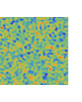
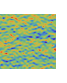
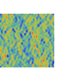
(a)	(b)	(c)

Figure 2.1: Statistical anisotropy. (a). This simulation corresponds to the statistical isotropic case $g_{\zeta}=0$. (b). In contrast, this simulation corresponds to the statistical anisotropic case with $g_{\zeta}=1$, $\hat{{\mathbf{d}}}$ pointing along the horizontal direction and setting to zero the isotropic part. (c). Same as in (b) but with $\hat{{\mathbf{d}}}$ pointing along the vertical direction. (Courtesy of Mindaugas Karčiauskas).

In some different studies, the mean-square CMB perturbation in opposite hemispheres has been measured, to see if there is any difference between hemispheres. Quite recent works [62, 63, 86] find a difference of order ten percent, for a certain choice of the hemispheres, with statistical significance at the $99\%$ level. Given the difficulty of handling systematic uncertainties it would be premature to regard the evidence for this hemispherical anisotropy as completely overwhelming. Nevertheless, what would hemispherical anisotropy imply for the curvature perturbation? Focussing on a small patch of sky, the statistical anisotropy of the curvature perturbation implies that the mean-square temperature perturbation within a given small patch will in general depend on the direction of that patch. This is because the mean square within such a patch depends upon the mean square of the curvature perturbation in a small planar region of space perpendicular to the line of sight located at last scattering. But the mean-square temperature will be the same in patches at opposite directions in the sky, because they explore the curvature perturbation $\zeta({\mathbf{k}})$ in the same ${\mathbf{k}}$-plane and the spectrum ${{\cal P}_{\zeta}}({\mathbf{k}})$ is invariant under the change ${\mathbf{k}}\to-{\mathbf{k}}$. It follows that statistical anisotropy of the curvature perturbation cannot by itself generate a hemispherical anisotropy. We may then conclude that hemispherical anisotropy of the CMB temperature requires statistical inhomogeneity of the curvature perturbation. Then ${\langle{\zeta({\bf k_{1}})\zeta({\bf k_{2}})}\rangle}$ is not proportional to $\delta^{3}({\bf k_{1}}+{\bf k_{2}})$ [41].

 SECTION 2.5      Conclusions

In this chapter we have presented the statistical description of primordial curvature perturbation $\zeta$. This framework allows us to define statistical descriptors, which provides a bridge between theory and observation. The relevant parameters that parametrize these statistical descritors are: the spectrum amplitude ${{\cal P}_{\zeta}}^{1/2}$, the spectral index $n_{\zeta}$, the levels of non-gaussianity $f_{\rm NL}$, $\tau_{\rm NL}$ and $g_{\rm NL}$ and the level of statistical anisotropy $g_{\zeta}$. Some of these parameters have an upper bound from observation, so it is very important to study theoretical models that successfully reproduce these observations. To study these theoretical aspects, we have presented a poweful tool to calculate the primordial cuvature pertubation $\zeta$ and all its statistical descriptors; such a tool is usully called the $\delta N$ formalism. In the next two chapters we will see how to work out this formalism.

Chapter 3          ON THE ISSUE OF THE $\zeta$ SERIES CONVERGENCE AND LOOP CORRECTIONS IN THE GENERATION OF OBSERVABLE PRIMORDIAL NON- GAUSSIANITY IN SLOW-ROLL INFLATION: THE BISPECTRUM

 SECTION 3.1      Introduction

Since COBE [158] discovered and mapped the anisotropies in the temperature of the cosmic microwave background radiation [199], many balloon and satellite experiments have refined the measurements of such anisotropies, reaching up to now an amazing combined precision. The COBE sequel has continued with the WMAP satellite [159] which has been able to measure the temperature angular power spectrum up to the third peak with unprecedent precision [90], and increase the level of sensitivity to primordial non-gaussianity in the bispectrum by two orders of magnitude compared to COBE [118, 119]. The next-to-WMAP satellite, PLANCK [59], which was launched in may of 2009, is expected to precisely measure the temperature angular power spectrum up to the eighth peak [206], and improve the level of sensitivity to primordial non-gaussianity in the bispectrum by one order of magnitude compared to WMAP [120].

Because of the progressive improvement in the accuracy of the satellite measurements described above, it is pertinent to study cosmological inflationary models that generate significant (and observable) levels of non-gaussianity. An interesting way to address the problem involves the $\delta\textit{N}$ formalism [52, 139, 142, 181, 182, 202], which can be employed to give the levels of non-gaussianity $f_{NL}$ [142] and $\tau_{NL}$ [6, 31] in the bispectrum $B_{\zeta}$ and trispectrum $T_{\zeta}$ of the primordial curvature perturbation $\zeta$ respectively. Such non-gaussianity levels are given, for slow-roll inflationary models, in terms of the local evolution of the universe under consideration, as well as of the $n$-point correlators, evaluated a few Hubble times after horizon exit, of the perturbations $\delta\phi_{i}$ in the scalar fields that determine the dynamics of such a universe during inflation.

In the $\delta\textit{N}$ formalism for slow-roll inflationary models, the primordial curvature perturbation $\zeta(\textbf{x},t)$ is written as a Taylor series in the scalar field perturbations $\delta\phi_{i}(\textbf{x},t_{\star})$ evaluated a few Hublle times after horizon exit,

$$\zeta(t,\textbf{x}) = \sum_{I}N_{I}(t)\delta\phi_{I}(\textbf{x},t_{\star})-\sum_{I}N_{I}(t)\langle\delta\phi_{I}(\textbf{x},t_{\star})\rangle+$$ (3.1)

$$+\frac{1}{2}\sum_{IJ}N_{IJ}(t)\delta\phi_{I}(\textbf{x},t_{\star})\delta\phi_{J}(\textbf{x},t_{\star})-\frac{1}{2}\sum_{IJ}N_{IJ}(t)\langle\delta\phi_{I}(\textbf{x},t_{\star})\delta\phi_{J}(\textbf{x},t_{\star})\rangle+$$

$$+\frac{1}{3!}\sum_{IJK}N_{IJK}(t)\delta\phi_{I}(\textbf{x},t_{\star})\delta\phi_{J}(\textbf{x},t_{\star})\delta\phi_{k}(\textbf{x},t_{\star})$$

$$- \frac{1}{3!}\sum_{IJK}N_{IJK}(t)\langle\delta\phi_{I}(\textbf{x},t_{\star})\delta\phi_{J}(\textbf{x},t_{\star})\delta\phi_{K}(\textbf{x},t_{\star})\rangle+$$

$$+...\;,$$

It is in this way that the correlation functions of $\zeta$ (for instance, $\langle\zeta_{\bf k_{1}}\zeta_{\bf k_{2}}\zeta_{\bf k_{3}}\rangle$) can be obtained in terms of series, as often happens in Quantum Field Theory where the probability amplitude is a series whose possible truncation at any desired order is determined by the coupling constants of the theory. A highly relevant question is that of whether the series for $\delta N$ converges in cosmological perturbation theory and whether it is possible in addition to find some quantities that determine the possible truncation of the series, which in this sense would be analogous to the coupling constants in Quantum Field Theory. In general such quantities will depend on the specific inflationary model; the series then cannot be simply truncated at some order until one is sure that it does indeed converge, and besides, one has to be careful not to forget any term that may be leading in the series even if it is of higher order in the coupling constant. This issue has not been investigated in the present literature, and generally the series has been truncated to second- or third-order neglecting in addition terms that could be the leading ones [5, 6, 22, 31, 40, 142, 181, 188, 211, 225, 226, 228].

The most studied and popular inflationary models nowadays are those of the slow-roll variety with canonical kinetic terms [137, 140, 141], because of their simplicity and because they easily satisfy the spectral index requirements for the generation of large-scale structures. One of the usual predictions from inflation and the theory of cosmological perturbations is that the levels of non-gaussianity in the primordial perturbations are expected to be unobservably small when considering this class of models [22, 127, 148, 188, 189, 190, 191, 211, 226, 228]. This fact leads us to analyze the cosmological perturbations in the framework of first-order cosmological perturbation theory. Non-gaussian characteristics are then suppressed since the non-linearities in the inflaton potential and in the metric perturbations are not taken into account. The non-gaussian characteristics are actually present and they are made explicit if second-order [143] or higher-order corrections are considered.

The whole literature that encompasses the slow-roll inflationary models with canonical kinetic terms reports that the non- gaussianity level $f_{NL}$ is expected to be very small, being of the order of the slow-roll parameters $\epsilon_{i}$ and $\eta_{i}$, ($\epsilon_{i},|\eta_{i}|\ll 1$) [22, 148, 191, 211, 226]. These works have not taken into account either the convergence of the series for $\zeta$ nor the possibility that loop corrections dominate over the tree level ones in the $n$-point correlators. Our main result in this chapter is the recognition of the possible convergence of the $\zeta$ series, and the existence of some “coupling constants” that determine the possible truncation of the $\zeta$ series at any desired order. When this situation is encountered in a subclass of small-field slow-roll inflationary models with canonical kinetic terms, the one-loop corrections may dominate the series when calculating either the spectrum $P_{\zeta}$, or the bispectrum $B_{\zeta}$. This in turn may generate sizeable and observable levels of non-gaussianity in total contrast with the general claims found in the present literature.

The layout of the chapter is the following: Section 3.2 is devoted to the issue of the $\zeta$ series convergence and loop corrections in the framework of the $\delta N$ formalism. The presentation of the current knowledge about primordial non-gaussianity in slow-roll inflationary models is given in Section 3.3. A particular subclass of small-field slow- roll inflationary models is the subject of Section 3.4 as it is this subclass of models that generate significant levels of non- gaussianity. The available parameter space for this subclass of models is constrained in Section 3.5 by taking into account some observational requirements such as the COBE normalisation, the scalar spectral tilt, and the minimal amount of inflation. Another requirement of methodological nature, the possible tree-level or one-loop dominance in $P_{\zeta}$ and/or $B_{\zeta}$, is considered in this section. The level of non-gaussianity $f_{NL}$ in the bispectrum $B_{\zeta}$ is calculated in Section 3.6 for models where $\zeta$ is generated during inflation; a comparison with the current literature is made. Section 3.7 is devoted to central issues in the consistency of the approach followed such as satisfying necessary conditions for the convergence of the $\zeta$ series and working in a perturbative regime. Finally in Section 3.8 we conclude. As regards the level of non-gaussianity $\tau_{NL}$ in the trispectrum $T_{\zeta}$, it will be studied in the following Chapter.

 SECTION 3.2      $\zeta$ series convergence and loop corrections

In order to calculate $\zeta(t,{\bf x})$ from Eq. (2.12), we need information about the physical content of the Universe at times $t$ and $t_{\rm in}$. By choosing the initial time $t_{\rm in}$ a few Hubble times after the cosmologically relevant scales leave the horizon during inflation $t_{\rm in}=t_{\star}$, and the final time $t$ corresponding to a slice of uniform energy density, we recognize that $N$, for slow-roll inflationary models, is completely parametrized by the values a few Hubble times after horizon exit of the scalar fields $\phi_{i}$ present during inflation and the energy density at the time at which one wishes to calculate $\zeta$:

$$\zeta(t,{\bf x})\equiv N(\rho(t),\phi_{1}(t_{\star},{\bf x}),\phi_{2}(t_{\star},{\bf x}),...)-N(\rho(t),\phi_{1}(t_{\star}),\phi_{2}(t_{\star}),...)\,.$$ (3.2)

The previous expression can be Taylor-expanded around the unperturbed background values for the scalar fields $\phi_{i}$ and suitably redefined so that $\langle\zeta(t,{\bf x})\rangle=0$. Thus,

$$\zeta(t,\textbf{x}) = \sum_{I}N_{I}(t)\delta\phi_{I}(\textbf{x},t_{\star})-\sum_{I}N_{I}(t)\langle\delta\phi_{I}(\textbf{x},t_{\star})\rangle+$$ (3.3)

$$+\frac{1}{2}\sum_{IJ}N_{IJ}(t)\delta\phi_{I}(\textbf{x},t_{\star})\delta\phi_{J}(\textbf{x},t_{\star})-\frac{1}{2}\sum_{IJ}N_{IJ}(t)\langle\delta\phi_{I}(\textbf{x},t_{\star})\delta\phi_{J}(\textbf{x},t_{\star})\rangle+$$

$$+\frac{1}{3!}\sum_{IJK}N_{IJK}(t)\delta\phi_{I}(\textbf{x},t_{\star})\delta\phi_{J}(\textbf{x},t_{\star})\delta\phi_{k}(\textbf{x},t_{\star})$$

$$- \frac{1}{3!}\sum_{IJK}N_{IJK}(t)\langle\delta\phi_{I}(\textbf{x},t_{\star})\delta\phi_{J}(\textbf{x},t_{\star})\delta\phi_{K}(\textbf{x},t_{\star})\rangle+$$

$$+...\;,$$

where the $\delta\phi_{i}(t_{\star},{\bf x})$ are the scalar field perturbations in the flat slice a few Hubble times after horizon exit, whose spectrum amplitude is given by [33]

$$\mathcal{P}^{1/2}_{\delta\phi_{i}}=\frac{H_{\star}}{2\pi}\,,$$ (3.4)

and the notation for the $N$ derivatives is $N_{i}\equiv\frac{\partial N}{\partial\phi_{i}}$, $N_{ij}\equiv\frac{\partial^{2}N}{\partial\phi_{i}\partial\phi_{j}}$, and so on.

The expression in Eq. (3.3) has been used to calculate the statistical descriptors of $\zeta$ at any desired order in cosmological perturbation theory by consistently truncating the series [142]. For instance, by truncating the series at first order, the amplitude of the spectrum $P_{\zeta}$ of $\zeta$ defined in Eqs. (2.20) and (2.35) is given by [181]

$$\mathcal{P}_{\zeta}=\left(\frac{H_{\star}}{2\pi}\right)^{2}\sum_{i}N_{i}^{2}\,,$$ (3.5)

which in turn gives the well known formula for the spectral index [181]:

$$n_{\zeta}-1=-2\epsilon-2m_{P}^{2}\frac{\sum_{ij}V_{i}N_{j}N_{ij}}{V\sum_{i}N_{i}^{2}}\,,$$ (3.6)

where a subindex $i$ in $V$ means a derivative with respect to the $\phi_{i}$ field, and being $\epsilon$ one of the slow-roll parameters defined by $\epsilon=-\dot{H}/H^{2}$, $m_{P}=(8\pi G)^{-2}$ the reduced Planck mass, and $V$ the scalar inflationary potential. Analogously, the level of non-gaussianity $f_{NL}$ in the bispectrum $B_{\zeta}$ of $\zeta$ defined in Eqs. (2.21) and (2.31) is obtained by truncating the series at second order and assuming that the scalar field perturbations $\delta\phi_{i}$ are perfectly gaussian [142]:

$$\frac{6}{5}f_{NL}=\frac{\sum_{ij}N_{i}N_{j}N_{ij}}{\left[\sum_{i}N_{i}^{2}\right]^{2}}+\mathcal{P}_{\zeta}\frac{\sum_{ijk}N_{ij}N_{jk}N_{ki}}{\left[\sum_{i}N_{i}^{2}\right]^{3}}\ln(kL)\,.$$ (3.7)

In the last expression the $\ln(kL)$ factor is of order one, $L$ being the infrared cutoff when calculating the stochastic properties in a minimal box [27, 138].

The truncated series methodology has proved to be powerful and reliable at reproducing successfully the level of non-gaussianity $f_{NL}$ in single-field slow-roll models [189] and in the curvaton scenario [31]. Nevertheless, for more general models, how reliable is it to truncate the series at some order? In the first place, from Eq. (3.3) it is impossible to know whether the series converges until the $N$ derivatives are explicitly calculated and the convergence radius is obtained; obviously if the series is not convergent at all, the expansion in Eq. (3.3) is meaningless. Without any proof of the contrary, the current assumption in the literature [3, 6, 22, 31, 40, 142, 181, 188, 211, 225, 226, 228] has been that the $\zeta$ series is convergent. In addition, supposing that the convergence radius is finally known, the truncation at any desired order would again be meaningless if some leading terms in the series get excluded. Such a situation might easily happen if each ${\bf x}$-dependent term in the $\zeta$ series is considered smaller than the previous one, which indeed is the standard assumption [3, 6, 22, 31, 40, 142, 181, 188, 211, 225, 226, 228], but which is not a universal fact.

When studying the series through a diagrammatic approach [39], in an analogous way to that for Quantum Field Theory via Feynman diagrams, the first-order terms in the spectral functions are called the tree-level terms. Examples of these tree-level terms are those in Eqs. (3.5) and (3.6), and the first one in Eq. (3.7). Higher-order corrections, such as that which contributes with the second term in Eq. (3.7), are called the loop terms because they involve internal momentum integrations. The statistical descriptors of $\zeta$ has been so far studied by naively neglecting the loop corrections against the tree-level terms [3, 6, 22, 31, 40, 142, 181, 188, 211, 225, 226, 228]; nevertheless, as might happen in Quantum Field Theory, eventually some loop corrections could be bigger than the tree-level terms, so it is essential to properly study the possible $n$-loop dominance in the spectral functions.

 SECTION 3.3      Non-gaussianity in slow-roll inflation

The most frequent class of inflationary models found in the literature are those which satisfy the so called slow-roll conditions, as these very simple models easily meet the spectral index observational requirements discussed in Subsection 2.4 for the generation of large-scale structures.

The slow-roll conditions for single-field inflationary models with canonical kinetic terms read

$$\dot{\phi}^{2} \ll V(\phi)\,,$$ (3.8)

$$|\ddot{\phi}| \ll |3H\dot{\phi}|\,,$$ (3.9)

where $\phi$ is the inflaton field and $V(\phi)$ is the scalar field potential. On defining the slow-roll parameters $\epsilon$ and $\eta_{\phi}$ as [140]

$$\epsilon \equiv -\frac{\dot{H}}{H^{2}}\,,$$ (3.10)

$$\eta_{\phi} \equiv \epsilon-\frac{\ddot{\phi}}{H\dot{\phi}}\,,$$ (3.11)

the slow-roll conditions in Eqs. (3.8) and (3.9) translate into strong constraints for the slow-roll parameters: $\epsilon,|\eta_{\phi}|\ll 1$, which actually become $\epsilon,|\eta_{\phi}|\mbox{\raisebox{-2.71246pt}{~{}$\stackrel{{\scriptstyle\mbox{$<$}}}{{\sim}}$~{}}}10^{-2}$ in view of Eq. (3.6) for single-field inflation:

$$n_{\zeta}-1=2\eta_{\phi}-6\epsilon\,,$$ (3.12)

and the observational requirements presented in Subsection 2.4.

Multifield slow-roll models may also be characterized by a set of slow-roll parameters which generalize those in Eqs. (3.10) and (3.11) [141]:

$$\epsilon_{i} \equiv \frac{m_{P}^{2}}{2}\left(\frac{V_{i}}{V}\right)^{2}\,,$$ (3.13)

$$\eta_{i} \equiv m_{P}^{2}\frac{V_{ii}}{V}\,.$$ (3.14)

By writing the slow-roll parameters in terms of derivatives of the scalar potential, as in the latter two expressions, we realize that the slow-roll conditions require very flat potentials to be met.

The level of non-gaussianity $f_{NL}$ in slow-roll inflationary models with canonical kinetic terms has been studied both for single-field [148] and for multiple-field inflation [22, 211, 226], assuming $\zeta$ series convergence and considering only the tree-level terms both in $P_{\zeta}$ and in $B_{\zeta}$. What these works find is a strong dependence on the slow-roll parameters $\epsilon_{i}$ and $\eta_{i}$; for instance, Ref. [148] gives us for single-field models:

$$\frac{6}{5}f_{NL}=\epsilon(1+f)+2\epsilon-\eta_{\phi}\,,$$ (3.15)

where $f$ is a function of the shape of the wavevectors triangle within the range $0\leq f\leq 5/6$. Refs. [21, 138] show that in such a case the inclusion of loop corrections is unnecessary because the latter are so small compared to the tree-level terms. Thus, $f_{NL}$ in single-field models with canonical kinetic terms is slow-roll suppressed and, therefore, unobservably small. As regards the multifield models, $f_{NL}$ was shown, first in the case of two- field inflation with separable potential [211] and later for multiple-field inflation with separable [22] and non-separable [226] potentials, to be a rather complex function of the slow-roll parameters and the scalar potential that in most of the cases ends up being slow-roll suppressed. Only for models with a sharply curved trajectory in field space might the $f_{NL}$ be at most of order one, the only possible examples to date being the models of Refs. [3, 28, 29, 37]. Again, such predictions are based on the assumptions that the $\zeta$ series is convergent and that the tree-level terms are the leading ones, so they might be badly violated if loop corrections are considered.

Following a parallel treatment to that in Ref. [211], the level of non-gaussianity $\tau_{NL}$ is calculated in Ref. [188] for multifield slow-roll inflationary models with canonical kinetic terms, separable potential, and assuming convergence of the $\zeta$ series and tree-level dominance. From reaching similar conclusions to those found for the $f_{NL}$ case, the $\tau_{NL}$ is slow-roll suppressed in most of the cases although it might be of order one if the trajectory in field space is sharply curved. Nevertheless, as we will shown in the next chapter, there may be a big enhancement in $\tau_{\rm NL}$ if loop corrections are taken into account.

Finally, it is worth mentioning that there are other classes of models where the levels of non-gaussianity $f_{NL}$ and $\tau_{NL}$ are big enough to be observable. Some of these models correspond to general langrangians with non-canonical kinetic terms ($k$-inflation [12], DBI inflation [195], ghost inflation [11], etc.), where the sizeable levels of non-gaussianity have mostly a quantum origin, i.e. their origin relies on the quantum correlators of the field perturbations a few Hubble times after horizon exit. Non-gaussianity in $B_{\zeta}$ has been studied in these models for the single-field case [42, 187] and also for the multifield case [16, 68, 124, 125]. A recent paper discusses the non-gaussianity in $T_{\zeta}$ for these general models for single-field inflation [15]. In contrast, there are some other models where the large non-gaussianities have their origin in the field dynamics at the end of inflation [26, 135]; nice examples of this proposal are studied for instance in Refs. [151, 152, 179, 180]. However, since the inflationary models of the slow-roll variety with canonical kinetic terms are the simplest, the most popular, and the best studied so far although, in principle, the non-gaussianity statistical descriptors are too small to ever be observable, it is very interesting to consider the possibility of having an example of such models which does generate sizeable and observable values for $f_{NL}$ and $\tau_{\rm NL}$. This appealing possibility will be the subject of the following sections and also the next chapter.

 SECTION 3.4      A subclass of small-field slow-roll inflationary models

According to the classification of inflationary models proposed in Ref. [57], the small-field models are those of the form that would be expected as a result of spontaneous symmetry breaking, with a field initially near an unstable equilibrium point (usually taken to be at the origin) and rolling toward a stable minimum $\langle\phi\rangle\neq 0$. Thus, inflation occurs when the field is small relative to its expectation value $\phi\ll\langle\phi\rangle$. Some interesting examples are the original models of new inflation [8, 128], modular inflation from string theory [55], natural inflation [64], and hilltop inflation [32]. As a result, the inflationary potential for small-field models may be taken as

$$V=\sum_{i}\Lambda_{i}\left[1-\left(\frac{\phi_{i}}{\mu_{i}}\right)^{p}\right]\,,$$ (3.16)

where the subscript $i$ here denotes the relevant quantities of the $i$th field, $p$ is the same for all fields, and $\Lambda_{i}$ and $\mu_{i}$ are the parameters describing the height and tilt of the potential of the $i$th field.

Figure 3.1: Our small-field slow-roll potential of Eq. (3.17) with $\eta_{\phi},\eta_{\sigma}<0$. The inflaton starts near the maximum and moves away from the origin following the $\sigma=0$ trajectory depicted with the solid black line. (This figure has been taken from Ref. [5]).

While Ref. [2] studies the spectrum of $\zeta$ for general values of the parameter $p$ and an arbitrary number of fields, assuming $\zeta$ series convergence and tree-level dominance, we will specialize to the $p=2$ case for two fields $\phi$ and $\sigma$:

$$V=V_{0}\left(1+\frac{1}{2}\eta_{\phi}\frac{\phi^{2}}{m_{P}^{2}}+\frac{1}{2}\eta_{\sigma}\frac{\sigma^{2}}{m_{P}^{2}}\right)\,,$$ (3.17)

where we have traded the expressions

$$\Lambda_{1}+\Lambda_{2} {\rm for} V_{0}\,,$$ (3.18)

$$\frac{\Lambda_{1}}{\mu_{1}^{2}} {\rm for} -V_{0}\frac{\eta_{\phi}}{2m_{P}^{2}}\,,$$ (3.19)

and

$$\frac{\Lambda_{2}}{\mu_{2}^{2}}\;\;\;{\rm for}\;\;\;-V_{0}\frac{\eta_{\sigma}}{2m_{P}^{2}}\,.$$ (3.20)

By doing this, and assuming that the first term in Eq. (3.17) dominates, $\eta_{\phi}<0$ and $\eta_{\sigma}<0$ become the usual $\eta$ slow-roll parameters associated with the fields $\phi$ and $\sigma$.

We have chosen for simplicity the $\sigma=0$ trajectory (see Fig. 3.1) since in that case the potential in Eq. (3.17) reproduces for some number of e-folds the hybrid inflation scenario [129] where $\phi$ is the inflaton and $\sigma$ is the waterfall field. Non-gaussianity in such a model has been studied in Refs. [3, 61, 142, 143, 207, 228]; in particular, Ref. [142] used a one-loop correction to conjecture that $f_{NL}$ in this model would be sizeable only if $\zeta$ was not generated during inflation, which turns out not to be a necessary requirement as we will show later [43, 175]. Ref. [3], in contrast, works only at tree-level with the same potential as Eq. (3.17) but relaxing the $\sigma=0$ condition, finding that values for $f_{NL}\sim\mathcal{O}(1)$ are possible for a small set of initial conditions and assuming a saddle-point-like form for the potential ($\eta_{\phi}<0$ and $\eta_{\sigma}>0$).

 SECTION 3.5      Constraints for having a reliable parameter space

We will explore now the constraints that the model must satisfy before we calculate the level of non-gaussianity $f_{NL}$. Our guiding idea will be the consideration of the role that the tree-level terms and one-loop corrections in $P_{\zeta}$ and $B_{\zeta}$ have in the determination of the available parameter space. Only after calculating $f_{NL}$ in Section 3.6 will we come back to the discussion of the consistency of the approach followed in the present section by studying the $\zeta$ series convergence and the validity of the truncation at one loop level.

3.5.1     Tree-level or one-loop dominance: $f_{\rm NL}$

Since we are considering a slow-roll regime, the evolution of the background $\phi$ and $\sigma$ fields in such a case is given by the Klein-Gordon equation

$$\ddot{\phi}+3H\dot{\phi}+V_{\phi}=0\,,$$ (3.21)

supplemented with the slow-roll condition in Eq. (3.9). This leads to

$$\phi(N) = \phi_{\star}\exp(-N\eta_{\phi})\,,$$ (3.22)

$$\sigma(N) = \sigma_{\star}\exp(-N\eta_{\sigma})\,,$$ (3.23)

so the potential above leads to the following derivatives of $N$ with respect to $\phi_{\star}$ and $\sigma_{\star}$ for the $\sigma=0$ trajectory:

$$N_{\phi}=\frac{1}{\eta_{\phi}\phi_{\star}}\,,\hskip 11.38109ptN_{\sigma}=0\,,$$ (3.24)

$$N_{\phi\phi}=-\frac{1}{\eta_{\phi}\phi_{\star}^{2}}\,,\hskip 11.38109ptN_{\phi\sigma}=0\,,\hskip 11.38109ptN_{\sigma\sigma}=\frac{\eta_{\sigma}}{\eta_{\phi}^{2}\phi_{\star}^{2}}\exp[2N(\eta_{\phi}-\eta_{\sigma})]\,,$$ (3.25)

$$N_{\phi\phi\phi}=\frac{2}{\eta_{\phi}\phi_{\star}^{3}}\,,\hskip 11.38109ptN_{\phi\phi\sigma}=0\,,\hskip 11.38109ptN_{\sigma\sigma\phi}=-\frac{2\eta_{\sigma}^{2}}{\eta_{\phi}^{3}\phi_{\star}^{3}}\exp[2N(\eta_{\phi}-\eta_{\sigma})]\,,\hskip 8.53581ptN_{\sigma\sigma\sigma}=0\,,$$ (3.26)

$$...$$

$${\rm and\ so\ on}.$$

By means of the $\delta N$ formalism, we can make use of the above formulae to calculate the spectrum and the bispectrum of the curvature perturbation including the tree-level and the one-loop contributions when $|\eta_{\sigma}|>|\eta_{\phi}|$ (see Appendix A). This is the interesting case since, as will be shown in Section 3.6, it generates sizeable values for $f_{NL}$. Following the results in Appendix A, we will write down just the leading terms to the tree-level and one- loop contributions given in Eqs. (A.1), (A.7), (A.11) and (A.28).

$${\mathcal{P}}_{\zeta}^{tree} = \frac{1}{\eta_{\phi}^{2}\phi_{\star}^{2}}\left(\frac{H_{\star}}{2\pi}\right)^{2}\,,$$ (3.27)

$${\mathcal{P}}_{\zeta}^{1-loop} = \frac{\eta_{\sigma}^{2}}{\eta_{\phi}^{4}\phi_{\star}^{4}}\exp[4N(\eta_{\phi}-\eta_{\sigma})]\left(\frac{H_{\star}}{2\pi}\right)^{4}\ln(kL)\,,$$ (3.28)

$$B_{\zeta}^{tree} = -\frac{1}{\eta_{\phi}^{3}\phi_{\star}^{4}}\left(\frac{H_{\star}}{2\pi}\right)^{4}4\pi^{4}\left(\frac{\sum_{i}k_{i}^{3}}{\prod_{i}k_{i}^{3}}\right)\,,$$ (3.29)

$$B_{\zeta}^{1-loop} = \frac{\eta_{\sigma}^{3}}{\eta_{\phi}^{6}\phi_{\star}^{6}}\exp[6N(\eta_{\phi}-\eta_{\sigma})]\left(\frac{H_{\star}}{2\pi}\right)^{6}\ln(kL)4\pi^{4}\left(\frac{\sum_{i}k_{i}^{3}}{\prod_{i}k_{i}^{3}}\right)\,.$$ (3.30)

Because of the exponential factors in Eqs. (3.28) and (3.30), it might be possible that the one-loop corrections dominate over $P_{\zeta}$ and/or $B_{\zeta}$. There are three posibilities in complete connection with the position of the $\phi$ field when the cosmologically relevant scales are exiting the horizon:

Both $B_{\zeta}$ and $P_{\zeta}$ are dominated by the one-loop corrections

Comparing Eqs. (3.27) with (3.28) and Eqs. (3.29) with (3.30) we require in this case that

$$\frac{\eta_{\sigma}^{2}}{\eta_{\phi}^{2}}\exp[4N(|\eta_{\sigma}|-|\eta_{\phi}|)] \gg \frac{1}{\frac{1}{\phi_{\star}^{2}}\left(\frac{H_{\star}}{2\pi}\right)^{2}}\,,$$ (3.31)

$$\frac{\eta_{\sigma}^{3}}{\eta_{\phi}^{3}}\exp[6N(|\eta_{\sigma}|-|\eta_{\phi}|)] \gg \frac{1}{\frac{1}{\phi_{\star}^{2}}\left(\frac{H_{\star}}{2\pi}\right)^{2}}\,,$$ (3.32)

in which case only the first inequality is required. Employing the definition for the tensor to scalar ratio $r$ [137]:

$$r\equiv\frac{\mathcal{P}_{T}}{\mathcal{P}_{\zeta}}=\frac{\frac{8}{m_{P}^{2}}\left(\frac{H_{\star}}{2\pi}\right)^{2}}{\mathcal{P}_{\zeta}}\,,$$ (3.33)

$\mathcal{P}_{T}^{1/2}$ being the amplitude of the spectrum for primordial gravitational waves, we can write such an inequality as

$$\left(\frac{\phi_{\star}}{m_{P}}\right)^{2}\ll\frac{r\mathcal{P}_{\zeta}}{8}\frac{\eta_{\sigma}^{2}}{\eta_{\phi}^{2}}\exp[4N(|\eta_{\sigma}|-|\eta_{\phi}|)]\,.$$ (3.34)

From now on we will name the parameter window described by Eq. (3.34) as the low $\phi_{\star}$ region since the latter represents a region of allowed values for $\phi_{\star}$ limited by an upper bound.

$B_{\zeta}$ dominated by the one-loop correction and $P_{\zeta}$ dominated by the tree-level term

Comparing Eqs. (3.27) with (3.28) and Eqs. (3.29) with (3.30) we require in this case that

$$\frac{\eta_{\sigma}^{2}}{\eta_{\phi}^{2}}\exp[4N(|\eta_{\sigma}|-|\eta_{\phi}|)] \ll \frac{1}{\frac{1}{\phi_{\star}^{2}}\left(\frac{H_{\star}}{2\pi}\right)^{2}}\,,$$ (3.35)

$$\frac{\eta_{\sigma}^{3}}{\eta_{\phi}^{3}}\exp[6N(|\eta_{\sigma}|-|\eta_{\phi}|)] \gg \frac{1}{\frac{1}{\phi_{\star}^{2}}\left(\frac{H_{\star}}{2\pi}\right)^{2}}\,,$$ (3.36)

which combines to give, employing the definition for the tensor to scalar ratio $r$ introduced in Eq. (3.33),

$$\frac{r\mathcal{P}_{\zeta}}{8}\frac{\eta_{\sigma}^{2}}{\eta_{\phi}^{2}}\exp[4N(|\eta_{\sigma}|-|\eta_{\phi}|)]\ll\left(\frac{\phi_{\star}}{m_{P}}\right)^{2}\ll\frac{r\mathcal{P}_{\zeta}}{8}\frac{\eta_{\sigma}^{3}}{\eta_{\phi}^{3}}\exp[6N(|\eta_{\sigma}|-|\eta_{\phi}|)]\,.$$ (3.37)

From now on we will name the parameter window described by Eq. (3.37) as the intermediate $\phi_{\star}$ region since the latter represents a region of allowed values for $\phi_{\star}$ limited by both an upper and a lower bound.

Both $B_{\zeta}$ and $P_{\zeta}$ are dominated by the tree-level terms

Comparing Eqs. (3.27) with (3.28) and Eqs. (3.29) with (3.30) we require in this case that

$$\frac{\eta_{\sigma}^{2}}{\eta_{\phi}^{2}}\exp[4N(|\eta_{\sigma}|-|\eta_{\phi}|)] \ll \frac{1}{\frac{1}{\phi_{\star}^{2}}\left(\frac{H_{\star}}{2\pi}\right)^{2}}\,,$$ (3.38)

$$\frac{\eta_{\sigma}^{3}}{\eta_{\phi}^{3}}\exp[6N(|\eta_{\sigma}|-|\eta_{\phi}|)] \ll \frac{1}{\frac{1}{\phi_{\star}^{2}}\left(\frac{H_{\star}}{2\pi}\right)^{2}}\,,$$ (3.39)

in which case only the second inequality is required. Employing the definition for the tensor to scalar ratio $r$ introduced in Eq. (3.33), we can write such an inequality as

$$\left(\frac{\phi_{\star}}{m_{P}}\right)^{2}\gg\frac{r\mathcal{P}_{\zeta}}{8}\frac{\eta_{\sigma}^{3}}{\eta_{\phi}^{3}}\exp[6N(|\eta_{\sigma}|-|\eta_{\phi}|)]\,.$$ (3.40)

From now on we will name the parameter window described by Eq. (3.40) as the high $\phi_{\star}$ region, since the latter represents a region of allowed values for $\phi_{\star}$ limited by a lower bound.

3.5.2     Spectrum normalisation condition

The model must satisfy the COBE normalisation on the spectrum amplitude $\mathcal{P}^{1/2}_{\zeta}$ [35] considering that $\zeta$ is assumed to be generated during inflation. There exist two possibilities discussed right below.

$\zeta$ generated during inflation and $P_{\zeta}$ dominated by the one-loop correction

According to Eq. (3.28), and the tensor to scalar ratio $r$ definition in Eq. (3.33), we have in this case

$$\mathcal{P}_{\zeta}^{1-loop} = \frac{\eta_{\sigma}^{2}}{\eta_{\phi}^{4}\phi_{\star}^{4}}\exp[4N(|\eta_{\sigma}|-|\eta_{\phi}|)]\left(\frac{H_{\star}}{2\pi}\right)^{4}\ln(kL)$$ (3.41)

$$= \frac{\eta_{\sigma}^{2}}{\eta_{\phi}^{4}}\exp[4N(|\eta_{\sigma}|-|\eta_{\phi}|)]\left(\frac{m_{P}}{\phi_{\star}}\right)^{4}\left(\frac{r\mathcal{P}_{\zeta}}{8}\right)^{2}\ln(kL)\,,$$

which reduces to

$$\left(\frac{\phi_{\star}}{m_{P}}\right)^{4}=\left(\frac{r}{8}\right)^{2}\mathcal{P}_{\zeta}\frac{\eta_{\sigma}^{2}}{\eta_{\phi}^{4}}\exp[4N(|\eta_{\sigma}|-|\eta_{\phi}|)]\ln(kL)\,,$$ (3.42)

where $\mathcal{P}_{\zeta}$ must be replaced by the observed value presented in Subsection 2.4.

$\zeta$ generated during inflation and $P_{\zeta}$ dominated by the tree-level term

According to Eq. (3.27), and the tensor to scalar ratio $r$ definition in Eq. (3.33), we have in this case

$$\mathcal{P}_{\zeta}^{tree} = \frac{1}{\eta_{\phi}^{2}\phi_{\star}^{2}}\left(\frac{H_{\star}}{2\pi}\right)^{2}$$ (3.43)

$$= \frac{1}{\eta_{\phi}^{2}}\left(\frac{m_{P}}{\phi_{\star}}\right)^{2}\frac{r\mathcal{P}_{\zeta}}{8}\,,$$

which reduces to

$$\left(\frac{\phi_{\star}}{m_{P}}\right)^{2}=\frac{1}{\eta_{\phi}^{2}}\frac{r}{8}\,.$$ (3.44)

Notice that in such a situation, the value of the $\phi$ field when the cosmologically relevant scales are exiting the horizon depends exclusively on the tensor to scalar ratio $r$, once $\eta_{\phi}$ has been fixed by the spectral tilt constraint as we will see later.

3.5.3     Spectral tilt constraint

The combined 5-year WMAP + Type I Supernovae + Baryon Acoustic Oscillations data [119] constrain the value for the spectral tilt as

$$n_{\zeta}-1=-0.040\pm 0.014\,.$$ (3.45)

Here again we have two possibilities: $\mathcal{P}_{\zeta}$ is dominated either by the one-loop correction or by the tree-level term:

$P_{\zeta}$ dominated by the one-loop correction

In this case the usual spectral index formula at tree-level [181] gets modified to account for the leading one-loop correction:

$$n_{\zeta}-1=-4\epsilon-2m_{P}^{2}\frac{\sum_{ijk}V_{k}N_{ijk}N_{ij}}{V\sum_{ij}N_{ij}N_{ij}}+\left[\ln(kL)\right]^{-1}\,.$$ (3.46)

By making use of the derivatives in Eqs. (3.24), (3.25), and (3.26), we have

$$n_{\zeta}-1=-4\epsilon+4\eta_{\sigma}+\left[\ln(kL)\right]^{-1}\,,$$ (3.47)

which implies that the observed value for $n_{\zeta}$ is never reproduced in view of $\ln(kL)\sim\mathcal{O}(1)$. Moreover, when calculating the running spectral index $dn_{\zeta}/d\ln k$ from Eq. (3.47), we obtain

$$\frac{dn_{\zeta}}{d\ln k}=-\left[\ln(kL)\right]^{-2}\,,$$ (3.48)

which rules out the possibility that $P_{\zeta}$ is dominated by the one-loop correction since the calculated $dn_{\zeta}/d\ln k$ is far from the observationally allowed $2\sigma$ range of values: $-0.0728<dn_{\zeta}/d\ln k<0.0087$ [119].

$P_{\zeta}$ dominated by the tree-level term

Now the usual spectral index formula [181] applies:

$$n_{\zeta}-1=-2\epsilon-2m_{P}^{2}\frac{\sum_{ij}V_{i}N_{j}N_{ij}}{V\sum_{i}N_{i}^{2}}\,,$$ (3.49)

giving the following result once the derivatives in Eqs. (3.24), (3.25), and (3.26) have been used:

$$n_{\zeta}-1=-2\epsilon+2\eta_{\phi}\,.$$ (3.50)

The efect of the $\epsilon$ parameter may be discarded in the previous expression since, as often happens in small-field models [6, 32], $\epsilon$ is negligible being much less than $|\eta_{\sigma}|$:

$$\epsilon=\frac{m_{P}^{2}}{2}\frac{V_{\phi}^{2}+V_{\sigma}^{2}}{V^{2}}=|\eta_{\phi}|\left[\frac{1}{2}|\eta_{\phi}|\left(\frac{\phi}{m_{P}}\right)^{2}\right]\ll|\eta_{\phi}|<|\eta_{\sigma}|\,,$$ (3.51)

according to the prescription that the potential in Eq. (3.17) is dominated by the constant term. Thus, by using the central value for $n_{\zeta}-1$, we get

$$\eta_{\phi}=-0.020\,.$$ (3.52)

3.5.4     Amount of inflation

Because of the characteristics of the inflationary potential in Eq. (3.17), inflation is eternal in this model. However, Ref. [157] introduced the multi-brid inflation idea of Refs. [179, 180] so that the potential in Eq. (3.17) is achieved during inflation while a third field $\rho$ acting as a waterfall field is stabilized in $\rho=0$. During inflation $\rho$ is heavy and it is trapped with a vacuum expectation value equal to zero, so neglecting it during inflation is a good approximation. The end of inflation comes when the effective mass of $\rho$ becomes negative, which is possible to obtain if $V_{0}$ in the potential of Eq. (3.17) is replaced by

$$V_{0}=\frac{1}{2}G(\phi,\sigma)\rho^{2}+\frac{\lambda}{4}\left(\rho^{2}-\frac{\Sigma^{2}}{\lambda}\right)^{2}\,,$$ (3.53)

where

$$G(\phi,\sigma)=g_{1}\phi^{2}+g_{2}\sigma^{2}\,,$$ (3.54)

$\Sigma$ has some definite value and $g_{1}$, $g_{2}$, and $\lambda$ some coupling constants. The end of inflation actually happens on a hypersurface defined in general by [157, 180]

$$G(\phi,\sigma)=\Sigma^{2}\,.$$ (3.55)

In general the hypersurface in Eq. (3.54), defined by the end of inflation condition, is not a surface of uniform energy density. Because the $\delta N$ formalism requires the final slice to be of uniform energy density, we need to add a small correction term to the amount of expansion up to the surface where $\rho$ is destabilised. In addition, the end of inflation is inhomogeneous, which generically leads to different predictions from those obtained during inflation for the spectral functions [4, 135, 177]. In particular, large levels of non-gaussianity may be obtained by tunning the free parameters of the model. Specifically, by making $g_{1}/g_{2}\ll 1$, large values for $f_{NL}$ and $\tau_{NL}$ are obtained due to the end of inflation mechanism rather than due to the dynamics during slow-roll inflation [4, 98, 157].

Ref. [38] chose instead the case $g_{1}^{2}/g_{2}^{2}=\eta_{\phi}/\eta_{\sigma}$ such that the surface where $\rho$ is destabilised corresponds to a surface of uniform energy density. In this case all of the spectral functions are the same as those calculated in this thesis (see Refs. [38, 43, 175]), which in turn are valid at the final hypersurface of uniform energy density during slow-roll inflation. Thus, we have a definite mechanism to end inflation which, nevertheless, leaves intact the non-gaussianity generated during inflation.

It is well known that the number of e-folds of expansion from the time the cosmological scales exit the horizon to the end of inflation is presumably around but less than 62 [56, 140, 155, 220]. The slow-roll evolution of the $\phi$ field in Eq. (3.22) tells us that such an amount of inflation is given by

$$N=-\frac{1}{\eta_{\phi}}\ln\left(\frac{\phi_{end}}{\phi_{\star}}\right)\mbox{\raisebox{-2.71246pt}{~{}$\stackrel{{\scriptstyle\mbox{$<$}}}{{\sim}}$~{}}}62\,,$$ (3.56)

where $\phi_{end}$ is the value of the $\phi$ field at the end of inflation. Such a value depends noticeably on the coupling constants in Eq. (3.53). We will in this chapter not concentrate on the allowed parameter window for $g_{1}$, $g_{2}$, and $\lambda$. Instead, we will give an upper bound on $\phi$ during inflation, for the $\eta_{\phi}<0$ case, consistent with the potential in Eq. (3.17) and the end of inflation mechanism described above.

Keeping in mind the results of Ref. [13] which say that the ultraviolet cutoff in cosmological perturbation theory could be a few orders of magnitude bigger than $m_{P}$, we will tune the coupling constants in Eq. (3.53) so that inflation for $\eta_{\phi}<0$ comes to an end when $|\eta_{\phi}|\phi^{2}/2m_{P}^{2}\sim 10^{-2}$. This allows us to be on the safe side (avoiding large modifications to the potential coming from ultraviolet cutoff-suppressed non-renormalisable terms, and keeping the potential dominated by the constant $V_{0}$ term). Coming back to Eq. (3.56), we get then

$$N=\frac{1}{|\eta_{\phi}|}\ln\left[\left(\frac{2\times 10^{-2}}{|\eta_{\phi}|}\right)^{1/2}\frac{m_{P}}{\phi_{\star}}\right]\mbox{\raisebox{-2.71246pt}{~{}$\stackrel{{\scriptstyle\mbox{$<$}}}{{\sim}}$~{}}}62\,,$$ (3.57)

which leads to

$$\frac{\phi_{\star}}{m_{P}}\mbox{\raisebox{-2.71246pt}{~{}$\stackrel{{\scriptstyle\mbox{$>$}}}{{\sim}}$~{}}}\left(\frac{2\times 10^{-2}}{|\eta_{\phi}|}\right)^{1/2}\exp(-62|\eta_{\phi}|)\,.$$ (3.58)

 SECTION 3.6      Non-Gaussianity: $f_{NL}$

In this section we will calculate the level of non-gaussianity represented in the parameter $f_{NL}$ by taking into account the constraints presented in Subsections 3.5.2, 3.5.3, and 3.5.4, and the different $\phi_{\star}$ regions discussed in Subsection 3.5.1.

3.6.1     The low $\phi_{\star}$ region

This case is of no observational interest because $P_{\zeta}$ dominated by the one-loop correction is already ruled out by the observed spectral index and its running as shown in Subsection 3.5.3. In addition, the generated non-gaussianity is so big that it causes violation of the observational constraint $f_{NL}>-9$:

$$\frac{6}{5}f_{NL}=\frac{B_{\zeta}^{1-loop}}{4\pi^{4}\frac{\sum_{i}k_{i}^{3}}{\prod_{i}k_{i}^{3}}(\mathcal{P}_{\zeta}^{1-loop})^{2}}=-[\mathcal{P}_{\zeta}\ln(kL)]^{-1/2}\sim-2\times 10^{4}\,,$$ (3.59)

according to the expressions in Eqs. (2.35), (2.31), (3.28), and (3.30).

We want to remark that, although it is of no observational interest, this case represents the first example of large non- gaussianity in the bispectrum $B_{\zeta}$ of $\zeta$ for a slow-roll model of inflation with canonical kinetic terms. It is funny to realize that the model in this case is additionally ruled out because the observational constraint on $f_{NL}$ is violated by an excess and not by a shortfall as is currently thought [22, 148, 191, 211, 226].

3.6.2     The intermediate $\phi_{\star}$ region

The level of non-gaussianity, according to the expressions in Eqs. (2.35), (2.31), (3.27), and (3.30), is in this case given by

$$\frac{6}{5}f_{NL} = \frac{B_{\zeta}^{1-loop}}{4\pi^{4}\frac{\sum_{i}k_{i}^{3}}{\prod_{i}k_{i}^{3}}(\mathcal{P}_{\zeta}^{tree})^{2}}=\frac{\eta_{\sigma}^{3}}{\eta_{\phi}^{2}\phi_{\star}^{2}}\exp[6N(|\eta_{\sigma}|-|\eta_{\phi}|)]\left(\frac{H_{\star}}{2\pi}\right)^{2}\ln(kL)$$ (3.60)

$$= \frac{\eta_{\sigma}^{3}}{\eta_{\phi}^{2}}\exp[6N(|\eta_{\sigma}|-|\eta_{\phi}|)]\left(\frac{m_{P}}{\phi_{\star}}\right)^{2}\frac{r\mathcal{P}_{\zeta}}{8}\ln(kL)$$

$$= \eta_{\sigma}^{3}\exp[6N(|\eta_{\sigma}|-|\eta_{\phi}|)]\mathcal{P}_{\zeta}\ln(kL)\,,$$

$$\Rightarrow\frac{6}{5}f_{NL} \approx -2.457\times 10^{-9}|\eta_{\sigma}|^{3}\exp[300\ \ln(5.657\times 10^{-2}r^{-1/2})\left(|\eta_{\sigma}|-0.020\right)]\,,$$ (3.61)

where in the last line we have used expressions from Eqs. (3.44), (3.52), and (3.57).

Now, by implementing the spectral tilt constraint in Eq. (3.52) in the spectrum normalisation constraint in Eq. (3.44) and the amount of inflation constraint in Eq. (3.58), we conclude that the tensor to scalar ratio $r$ is bounded from below: $r\mbox{\raisebox{-2.71246pt}{~{}$\stackrel{{\scriptstyle\mbox{$>$}}}{{\sim}}$~{}}}2.680\times 10^{-4}$.

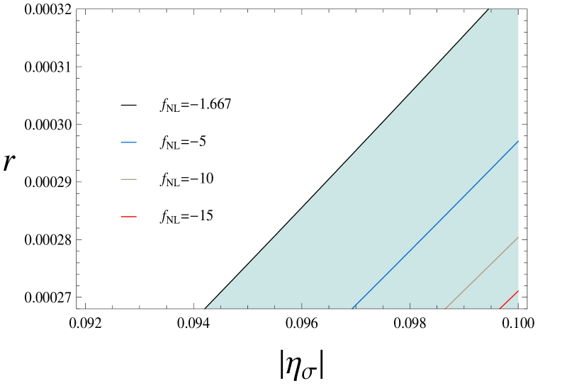
Figure 3.2: Contours of $f_{NL}$ in the $r$ vs $|\eta_{\sigma}|$ plot. The intermediate (high) $\phi_{\star}$ region corresponds to the shaded (white) region. The WMAP (and also PLANCK) observationally allowed $2\sigma$ range of values for negative $f_{NL}$, $-9<f_{NL}$, is completely inside the intermediate $\phi_{\star}$ region. Notice that the boundary line between the high and the intermediate $\phi_{\star}$ regions matches almost exactly the $f_{NL}=-1.667$ line.

In the plot $r$ vs $|\eta_{\sigma}|$ in figure 3.2, we show lines of constant $f_{NL}$ corresponding to the values $f_{NL}=-5,-10,-15$. We also show the high and intermediate $\phi_{\star}$ regions in agreement with the constraint in Eq. (3.37):

$$\frac{r\mathcal{P}_{\zeta}}{8}\frac{\eta_{\sigma}^{2}}{\eta_{\phi}^{2}}\exp[4N(|\eta_{\sigma}|-|\eta_{\phi}|)]\ll\left(\frac{\phi_{\star}}{m_{P}}\right)^{2}\ll\frac{r\mathcal{P}_{\zeta}}{8}\frac{\eta_{\sigma}^{3}}{\eta_{\phi}^{3}}\exp[6N(|\eta_{\sigma}|-|\eta_{\phi}|)]\,,$$

$$\Rightarrow\;\;8.139\times 10^{6}\ll|\eta_{\sigma}|^{3}\exp[300\ln(5.657\times 10^{-2}r^{-1/2})\left(|\eta_{\sigma}|-0.020\right)]\ll 8.210\times 10^{12}\,.$$ (3.62)

As is evident from the plot, the WMAP (and also PLANCK) observationally allowed $2\sigma$ range of values for negative $f_{NL}$, $-9<f_{NL}$, is completely inside the intermediate $\phi_{\star}$ region as required. More negative values for $f_{NL}$, up to $f_{NL}=-20.647$ are consistent within our framework for the intermediate $\phi_{\star}$ region, but they are ruled out from observation. Nevertheless, like for the low $\phi_{\star}$ region studied above, it is interesting to see a slow- roll inflationary model with canonical kinetic terms where the observational restriction on $f_{NL}$ may be violated by an excess and not by a shortfall. So we conclude that if $B_{\zeta}$ is dominated by the one-loop correction but $P_{\zeta}$ is dominated by the tree-level term, sizeable non-gaussianity is generated even if $\zeta$ is generated during inflation. We also conclude, from looking at the small values that the tensor to scalar ratio $r$ takes in figure 3.2 compared with the present technological bound $r\mbox{\raisebox{-2.71246pt}{~{}$\stackrel{{\scriptstyle\mbox{$>$}}}{{\sim}}$~{}}}10^{-3}$ [65], that for non-gaussianity to be observable in this model, primordial gravitational waves must be undetectable.

Notice that in oder to get positive values for $f_{NL}$, which is observationally more interesting in view of the results presented in Subsection 2.4, $\eta_{\sigma}$ should be positive according to Eq. (3.60). However, being $\eta_{\phi}$ negative in order to reproduce the observed spectral tilt, the argument of the exponential in Eq. (3.60) would be negative, making the $f_{NL}$ obtained too small to be observationally interesting. As regards the general case, in view of the previous reason being model dependent, we may only say that in order to get $f_{NL}$ positive when $B_{\zeta}$ is dominated by the one-loop corrections, $B_{\zeta}$ should be positive (based on the definition of $f_{NL}$ in Eq. (2.31)) which means that the maximum between $N_{\sigma\sigma}$ and $N_{\phi\phi}$ should be positive in view of Eq. (A.12).

Finally we want to point out that, by reducing our model to the single-field case, the consistency relation between $f_{NL}$ and $n_{\zeta}$ presented in Ref. [46]: $f_{NL}\sim\mathcal{O}(n_{\zeta}-1)$ is not violated since in that case $B_{\zeta}$ is never dominated by the one-loop corrections for slow-roll inflation as demonstrated in Ref. [138]. Thus, the level of non-gaussianity $f_{NL}$ for our model reduced to the single-field case is described by the high $\phi_{\star}$ region as shown below.

3.6.3     The high $\phi_{\star}$ region

This case is of no observational interest because, according to the expressions in Eqs. (2.35), (2.31), (3.27), (3.29), and (3.52), the non-gaussianity generated is too small to be observable:

$$\frac{6}{5}f_{NL}=\frac{B_{\zeta}^{tree}}{4\pi^{4}\frac{\sum_{i}k_{i}^{3}}{\prod_{i}k_{i}^{3}}(\mathcal{P}_{\zeta}^{tree})^{2}}=-\eta_{\phi}=0.020\,,$$ (3.63)

in agreement with the consistency relation of Ref. [46] for our model reduced to the single-field case, and with the general expectations of Refs. [22, 148, 191, 211, 226] for slow-roll inflationary models with canonical kinetic terms where only the tree-level contributions are considered.

 SECTION 3.7      Convergence of the $\zeta$ series and perturbative regime

In Sections 3.5 and 3.6 we have worked up to the one-loop diagrams in order to constrain the parameter space and find the level of non-gaussianity $f_{NL}$. It is time then to address the issue of the $\zeta$ series convergence and justify the existence of a perturbative regime so that the truncation of the series up to the one-loop order, for the model we have considered, is valid. A way to do that is by rederiving the $\zeta$ series in terms of $\delta\phi_{\star}$ and $\delta\sigma_{\star}$ by equating the unperturbed scalar potential to the perturbed one at the final time $t$; this of course is valid in view of the first slow-roll condition in Eq. (3.8) and the final slice being one of uniform energy density:

$$V_{0}\left\{1+\frac{1}{2}\eta_{\phi}\frac{\phi_{\star}^{2}}{m_{P}^{2}}\exp[-2N\eta_{\phi}]+\frac{1}{2}\eta_{\sigma}\frac{\sigma_{\star}^{2}}{m_{P}^{2}}\exp[-2N\eta_{\sigma}]\right\}$$

$$=V_{0}\left\{1+\frac{1}{2}\eta_{\phi}\frac{(\phi_{\star}+\delta\phi_{\star})^{2}}{m_{P}^{2}}\exp[-2(N+\delta N)\eta_{\phi}]+\frac{1}{2}\eta_{\sigma}\frac{(\sigma_{\star}+\delta\sigma_{\star})^{2}}{m_{P}^{2}}\exp[-2(N+\delta N)\eta_{\sigma}]\right\}\,.$$

From the previous expression it follows that

$$\eta_{\phi}\phi_{\star}^{2}\exp[-2N\eta_{\phi}]+\eta_{\sigma}\sigma_{\star}^{2}\exp[-2N\eta_{\sigma}]$$

$$=\eta_{\phi}(\phi_{\star}+\delta\phi_{\star})^{2}\exp[-2(N+\delta N)\eta_{\phi}]+\eta_{\sigma}(\sigma_{\star}+\delta\sigma_{\star})^{2}\exp[-2(N+\delta N)\eta_{\sigma}]\,,$$ (3.65)

which is easier to handle in terms of variables $x$ and $y$ defined as

$$x \equiv \frac{\delta\phi_{\star}}{\phi_{\star}}\,,$$ (3.66)

$$y \equiv \left[\frac{\eta_{\sigma}^{3}}{\eta_{\phi}^{3}}\frac{\sigma_{\star}^{2}}{\phi_{\star}^{2}}\left(1+\frac{\delta\sigma_{\star}}{\sigma_{\star}}\right)^{2}\exp[2N(\eta_{\phi}-\eta_{\sigma})]\right]^{1/2}\,.$$ (3.67)

Thus, the exponentials factors contaning $N$ (but not $\delta N$) are completely absorbed in $y$, and the expression in Eq. (3.65) looks as follows:

$$1+\frac{\eta_{\phi}^{2}}{\eta_{\sigma}^{2}}\frac{1}{\left(1+\frac{\delta\sigma_{\star}}{\sigma_{\star}}\right)^{2}}y^{2}=(1+x)^{2}\exp[-2\delta N\eta_{\phi}]+\frac{\eta_{\phi}^{2}}{\eta_{\sigma}^{2}}y^{2}\exp[-2\delta N\eta_{\sigma}]\,.$$ (3.68)

If we were able to solve for $\delta N$ in Eq. (3.68) in terms of $\eta_{\phi}$, $\eta_{\sigma}$, $x$, and $y$ (after making $\sigma_{\star}=0$), we could Taylor-expand around $x=0$ and $y=0$ reproducing the ${\bf x}$-dependent part of Eq. (3.3). This would be really good because the Taylor expansion would look so clean, in the sense that all the concerning exponential factors contaning $N$ which appear explicitely in Eq. (3.3) would already be absorbed in $y$, that the issue of truncating at some specific order in $\delta\phi_{\star}$ and $\delta\sigma_{\star}$ would be simply justified by requiring $|x|\ll 1$ and $|y|\ll 1$. Nevertheless, as is seen in Eq. (3.68), it is impossible to solve for $\delta N$ in terms of $\eta_{\phi}$, $\eta_{\sigma}$, $x$, and $y$ unless we make a Taylor expansion of the exponential functions aroud $\delta N=0$:

$$0 = \left\{\left[(1+x)^{2}-1\right]+\frac{\eta_{\phi}^{2}}{\eta_{\sigma}^{2}}y^{2}\left[1-\frac{1}{\left(1+\frac{\delta\sigma_{\star}}{\sigma_{\star}}\right)^{2}}\right]\right\}+$$ (3.69)

$$+\delta N\left[-2\eta_{\phi}(1+x)^{2}-2\frac{\eta_{\phi}^{2}}{\eta_{\sigma}}y^{2}\right]+\delta N^{2}\left[2\eta_{\phi}^{2}(1+x)^{2}+2\eta_{\phi}^{2}y^{2}\right]+...\,.$$

Notice that the Taylor expansion of the exponential functions is always convergent whatever the arguments of the exponentials are. Moreover, if the Taylor expansion derived from a function $f(x)$ converges, it converges precisely to $f(x)$ [200]. Thus, the expression in Eq. (3.69) is actually the same as the expression in Eq. (3.68).

Now, solving for $\delta N$ in terms of $\eta_{\phi}$, $\eta_{\sigma}$, $x$, and $y$, although possible in view of the expression in Eq. (3.69), is not an easy business. That is why we will truncate the series in Eq. (3.69) up to second order in $\delta N$ and solve the resultant quadratic equation. Notice that, since $\zeta\equiv\delta N-\langle\delta N\rangle$ and $\zeta\sim 10^{-5}$, we may truncate the series in Eq. (3.69) up to whatever order we wish and still reproduce $\zeta$ to high accuracy. Thus, the solution for the quadratic equation coming from the series in Eq. (3.69) after truncation at second order is:

$$\delta N \approx \Big{\{}\frac{1}{2}\left(1+x\right)^{2}+\frac{1}{2}\frac{\eta_{\phi}}{\eta_{\sigma}}y^{2}\pm\Big{\{}\left[\frac{1}{2}\left(1+x\right)^{2}+\frac{1}{2}\frac{\eta_{\phi}}{\eta_{\sigma}}y^{2}\right]^{2}-$$ (3.70)

$$-\frac{1}{2}\left\{\left[\left(1+x\right)^{2}-1\right]+\frac{\eta_{\phi}^{2}}{\eta_{\sigma}^{2}}y^{2}\left[1-\frac{1}{\left(1+\frac{\delta\sigma_{\star}}{\sigma_{\star}}\right)^{2}}\right]\right\}\left[\left(1+x\right)^{2}+y^{2}\right]\Big{\}}^{1/2}\Big{\}}\times$$

$$\times\left\{\eta_{\phi}\left[\left(1+x\right)^{2}+y^{2}\right]\right\}^{-1}\,.$$

If in addition we make Taylor expansions of the square root and the factor in the third line of the previous expression around $x=0$ and $y=0$:

$$\left\{\left[\frac{1}{2}\left(1+x\right)^{2}+\frac{1}{2}\frac{\eta_{\phi}}{\eta_{\sigma}}y^{2}\right]^{2}-\frac{1}{2}\left\{\left[\left(1+x\right)^{2}-1\right]+\frac{\eta_{\phi}^{2}}{\eta_{\sigma}^{2}}y^{2}\left[1-\frac{1}{\left(1+\frac{\delta\sigma_{\star}}{\sigma_{\star}}\right)^{2}}\right]\right\}\left[\left(1+x\right)^{2}+y^{2}\right]\right\}^{1/2}$$

$$=\frac{1}{2}-x^{2}+\frac{\eta_{\phi}}{2\eta_{\sigma}}\left\{1-\frac{\eta_{\phi}}{\eta_{\sigma}}\left[1-\frac{1}{\left(1+\frac{\delta\sigma_{\star}}{\sigma_{\star}}\right)^{2}}\right]\right\}y^{2}+...\,,$$ (3.71)

$$\left\{\eta_{\phi}\left[\left(1+x\right)^{2}+y^{2}\right]\right\}^{-1}=\frac{1}{\eta_{\phi}}\left[1-2x+3x^{2}-y^{2}+...\right]\,,$$ (3.72)

introducing them into Eq. (3.70), we end up with the following power series for $\delta N$:

$$\delta N\approx\frac{1}{\eta_{\phi}}\left(x-\frac{x^{2}}{2}+\frac{\eta_{\phi}^{2}}{2\eta_{\sigma}^{2}}y^{2}+...\right)\,,$$ (3.73)

where the $\pm$ symbol is changed to the $-$ sign so that $\delta N$ remains a perturbation, and the trajectory $\sigma=0$ is chosen. Coming back to the variables $\delta\phi_{\star}$ and $\delta\sigma_{\star}$ we see that Eq. (3.73) reproduces the ${\bf x}$-dependent part of Eq. (3.3) in view of Eqs. (3.24) and (3.25) up to second order in $\delta\phi_{\star}$ and $\delta\sigma_{\star}$:

$$\delta N\approx\frac{\delta\phi_{\star}}{\eta_{\phi}\phi_{\star}}-\frac{1}{2\eta_{\phi}}\left(\frac{\delta\phi_{\star}}{\phi_{\star}}\right)^{2}+\frac{\eta_{\sigma}}{2\eta_{\phi}^{2}}\left(\frac{\delta\sigma_{\star}}{\phi_{\star}}\right)^{2}\exp\left[2N\left(\eta_{\phi}-\eta_{\sigma}\right)\right]+...\,.$$ (3.74)

Eq. (3.73), although reliable only up to second order, tells us that the expected behaviour of $\delta N$ in terms of $\eta_{\phi}$, $\eta_{\sigma}$, $x$, and $y$ is indeed obtained. Moreover, from our previous discussion we know that $\delta N$ can be exactly written in terms of a series of $x$ and $y$ withouth the explicit appearance of the concerning exponential factors containing $N$. This is indeed partially confirmed up to third order when introducing Eqs. (3.24), (3.25), and (3.26) into the ${\bf x}$-dependent part of Eq. (3.3):

$$\delta N=\frac{1}{\eta_{\phi}}\left(x-\frac{x^{2}}{2}+\frac{\eta_{\phi}^{2}}{2\eta_{\sigma}^{2}}y^{2}+\frac{x^{3}}{3}-\frac{\eta_{\phi}}{3\eta_{\sigma}}xy^{2}+...\right)\,.$$ (3.75)

The bottom line of this discussion is that we have been able to identify two quantities that determine the truncation of the series up to some specific order. These two quantities are $x$ and $y$ which we could identify as the “coupling constants” of the theory in the context of Quantum Field Theory. By making $|x|\ll 1$ and $|y|\ll 1$ we can see from Eq. (3.75) that all the terms higher than second order in $x$ and $y$ are subleading compared to the second-order ones. As regards the first-order terms compared to the second-order ones, we see that the latter are not necessarily subleading compared to the former because of the non-existence of the first-order $y$ term and in view of $|y/x|\mbox{\raisebox{-2.71246pt}{~{}$\stackrel{{\scriptstyle\mbox{$<$}}}{{\sim}}$~{}}}1600$ from Eqs. (3.66) and (3.67) and the values for $\eta_{\phi}$, $\eta_{\sigma}$ and $N$ considered in Sections 3.5, 3.6 and 4.6. In the language of the Feynman-like diagrams [39], truncating $\delta N$ in Eq. (3.75) up to second order in $x$ and $y$ means considering only the leading diagrams at tree level and one loop which is what we have done in Sections 3.5, 3.6. In fact, $|x|\ll 1$ and $|y|\ll 1$ mean that

$$|x|\equiv\left|\frac{\delta\phi_{\star}}{\phi_{\star}}\right|\approx\left(\frac{H_{\star}}{2\pi}\right)\frac{1}{\phi_{\star}}\ll 1\,,$$ (3.76)

$$|y|\equiv\left\{\frac{\eta_{\sigma}^{3}}{\eta_{\phi}^{3}}\frac{\delta\sigma_{\star}^{2}}{\phi_{\star}^{2}}\exp[2N(\eta_{\phi}-\eta_{\sigma})]\right\}^{1/2}\approx\left\{\frac{\eta_{\sigma}^{3}}{\eta_{\phi}^{3}}\left(\frac{H_{\star}}{2\pi}\right)^{2}\frac{1}{\phi_{\star}^{2}}\exp[2N(\eta_{\phi}-\eta_{\sigma})]\right\}^{1/2}\ll 1\,,$$ (3.77)

which are well satisfied for the cases when $P_{\zeta}$ is dominated by the tree-level term (see Subsection 3.5.2 - Eq. (3.43) and Subsection 3.5.1 - Eq. (3.35)):

$$\left(\frac{H_{\star}}{2\pi}\right)\frac{1}{\phi_{\star}}=|\eta_{\phi}|\mathcal{P}_{\zeta}^{1/2}\approx 10^{-6}\,,\\$$ (3.78)

$$\left\{\frac{\eta_{\sigma}^{3}}{\eta_{\phi}^{3}}\left(\frac{H_{\star}}{2\pi}\right)^{2}\frac{1}{\phi_{\star}^{2}}\exp[2N(\eta_{\phi}-\eta_{\sigma})]\right\}^{1/2}\ll\left\{\frac{\eta_{\sigma}}{\eta_{\phi}}\exp[-2N(|\eta_{\sigma}|-|\eta_{\phi}|)]\right\}^{1/2}\mbox{\raisebox{-2.71246pt}{~{}$\stackrel{{\scriptstyle\mbox{$<$}}}{{\sim}}$~{}}}2\,.$$ (3.79)

By explicitly calculating the two-loop and three-loop diagrams for $P_{\zeta}$ and $B_{\zeta}$, and employing the results of Ref. [100], we have checked that the conditions $|x|\ll 1$ and $|y|\ll 1$ efectively make these diagrams subleading compared to the leading ones at one-loop level.

Finally, we will discuss the convergence of the $\zeta$ series in view of Eqs. (3.70), (3.71), and (3.72). We first note that the series in Eq. (3.71) is always convergent. As regards the series in Eq. (3.72), it will not be convergent at all while the function

$$\frac{1}{(1+x)^{2}+y^{2}}\approx\frac{1}{(1+x)^{2}+B^{2}x^{2}}\,,$$ (3.80)

with

$$B=\left(\frac{\eta_{\sigma}}{\eta_{\phi}}\right)^{3/2}\exp[N(\eta_{\phi}-\eta_{\sigma})]\,,$$ (3.81)

does not satisfy the following necessary condition [200]: for the Taylor series around $x=0$ of a function $f(x)$ to be convergent, it is necessary that the extension $f(z)$ to the complex plane of $f(x)$ is continous in a neighbourhood of $z=0$. If this is the case, and the Taylor series of $f(z)$ is indeed convergent, the convergence circle must either match or be inside the aforementioned neighbourhood. Of course, this is not a sufficient condition, but at least gives us a constraint on the possible values that $x$ may take.

Applying this condition to the expression in Eq. (3.80), we see that the extension of this function to the complex plane has poles for $(1+z)^{2}=-B^{2}z^{2}$ which leads to

$$z=\frac{\pm iB-1}{B^{2}+1}\,.$$ (3.82)

Therefore, the extension to the complex plane of Eq. (3.80) is continous for

$$|z|<\frac{B^{2}+1}{B^{2}+1}=1\,,$$ (3.83)

so the necessary condition for the convergence of the series in Eq. (3.72), and therefore for the convergence of the series in Eq. (3.70) which is what we are interested in, is given by $|x|<1$. Thus, such a necessary condition for the convergence of the $\zeta$ series is automatically satisfied once we choose $|x|\ll 1$, as we have seen above it is required for working in a perturbative regime.

 SECTION 3.8      Conclusions

Is it reasonable to study the primordial curvature perturbation $\zeta$ by identifying it with a truncated $\delta N$ series expansion? Is it actually possible to cut out with confidence such a series at some specific order? Is it true that all the slow-roll inflationary models with canonical kinetic terms produce primordial non-gaussianity supressed by the slow-roll parameters? Are the loop corrections in cosmological perturbation theory always smaller than the tree-level terms? We have addressed these questions in this chapter, answering all of them by paying particular attention to a special slow-roll inflationary model. The $\zeta$ series expansion is indeed a powerful tool to study the statistical descriptors of $\zeta$; nevertheless, we should seek for the convergence radius in order not to obtain results that actually have nothing to do with $\zeta$. We may cut out the series but, to be completely sure about the precision of our approximations, we have to study the conditions for the existence of a perturbative regime. Non-gaussianity in slow-roll inflationary models with canonical kinetic terms is not always suppressed by the slow-roll parameters; we have seen this at tree-level for $f_{NL}$ in Refs. [3, 37], and considering loop corrections for $f_{NL}$ in the prersent chapter and in Refs. [43, 38]. Particulary, we shown in this chapter that it is possible to attain very high, including observable, values for the level of non-gaussianity $f_{NL}$ associated with the bispectrum $B_{\zeta}$ of the primordial curvature perturbation $\zeta$, in a subclass of small-field slow-roll models of inflation with canonical kinetic terms. Such a result was obtained by taking care of loop corrections both in the spectrum $P_{\zeta}$ and the bispectrum $B_{\zeta}$ and assuming that the latter can dominate over the former; of course, this possibility is model dependent. More precisely, we can say that if $B_{\zeta}$ is dominated by the one-loop correction but $P_{\zeta}$ is dominated by the tree-level term, sizeable non-gaussianity is generated even if $\zeta$ is generated during inflation. What is interesting is that this kind of particular models are populary known to predict too small values for the level of non-gaussianity $f_{\rm NL}$, as small as the slow-roll parameters. Finally, as far as we have investigated, the loop corrections in cosmological perturbation theory are not always smaller than the tree-level terms; in fact, when they become the leading contributions, a surprising phenomenology appears in front of our eyes.

Chapter 4          ON THE ISSUE OF THE $\zeta$ SERIES CONVERGENCE AND LOOP CORRECTIONS IN THE GENERATION OF OBSERVABLE PRIMORDIAL NON- GAUSSIANITY IN SLOW-ROLL INFLATION: THE TRISPECTRUM

 SECTION 4.1      Introduction

The primordial curvature perturbation $\zeta$ [56, 140, 155, 220], and its $\delta N$ expansion [52, 139, 142, 181, 182, 202], was the subject of study in a previous chapter (see also [43]). We were interested in how well the convergence of the $\zeta$ series was understood, and if the traditional arguments to cut out the $\zeta$ series at second order [142, 228], keeping only the tree-level terms to study the statistical descriptors of $\zeta$ [5, 22, 37, 40, 188, 211, 226, 225, 227], were reliable. We argued that a previous study of the $\zeta$ series convergence, the viability of a perturbative regime, and the relative weight of the loop contributions against the tree- level terms, were completely necessary and in some cases surprising. For instance, the levels of non-gaussianity $f_{NL}$ and $\tau_{NL}$ in the bispectrum $B_{\zeta}$ and trispectrum $T_{\zeta}$ of $\zeta$ respectively, for slow-roll inflationary models with canonical kinetic terms [137, 140, 141], are usually thought to be of order $\mathcal{O}(\epsilon_{i},\eta_{i})$ [22, 211, 226] and $\mathcal{O}(r)$ [188, 192] respectively, were $\epsilon_{i}$ and $\eta_{i}$ are the slow-roll parameters with $\epsilon_{i},|\eta_{i}|\ll 1$ [141] and $r$ is the tensor to scalar ratio [137] with $r<0.22$ at the $95\%$ confidence level [119]. However, in order to reach such a conclusion, generic models were used where the loop contributions are comparatively suppressed and, therefore, the truncated $\delta N$ expansion may be used. Of course exceptions may occur, and in those cases it is crucial to check up to what order the truncated $\delta N$ expansion may be used, and which loop contributions are larger than the tree-level terms. In any of these cases, general models or exceptions, the question regarding the representation of $\zeta$ by the $\delta N$ expansion is a matter to discuss.

Refs. [5, 37] show that large, and observable, non-gaussianity in $B_{\zeta}$ is indeed possible for certain classes of slow-roll models with canonical kinetic terms and special trajectories in field space, relying only on the tree-level terms. Ref. [38] does the same for $B_{\zeta}$ and $T_{\zeta}$ but this time arguing that the loop corrections are always suppressed against the tree-level terms if the quantum fluctuations of the scalar fields do not overwhelm the classical evolution. Nonetheless, although the resultant phenomenology from papers in Refs. [5, 37, 38] is very interesting, the classicality argument used in Ref. [38] is very conservatively stated leading to too strong conclusions as we will argue later in this chapter. More research remains to be done to understand the role of the quantum diffusion and, being this beyond the scope of the present chapter, we will leave the discussion for a future research project. We addressed the $\zeta$ series convergence and the existence of a perturbative regime in the previous chapter, showing how important the requirements to guarantee those conditions are. Moreover, we showed that for a subclass of small-field slow-roll inflationary models with canonical kinetic terms, the one-loop correction to $B_{\zeta}$ might be much larger than the tree-level terms, giving as a result large, and observable, non-gaussianity parameterised by $f_{NL}$. The present chapter extends the analysis presented in the previous one to $T_{\zeta}$ showing, for the first time, that large and observable non-gaussianity parameterised by $\tau_{NL}$ is possible in slow-roll inflationary models with canonical kinetic terms due to loop effects, in total contrast with the usual belief based on the results of Refs. [188, 192]. In order to properly identify the non-gaussianity levels found in previous chapter and in the present one with those that are constrained by observation, we comment on the probability that an observer in an ensemble of realizations of the density field in our scenario sees a non-gaussian distribution. As we will show such a probability is non-negligible for the concave downward potential, making indeed the observation of the non-gaussianity studied in this chapter quite possible.

The layout of the chapter is the following: in Section 4.2 we make some aditional comments about ot the slow-roll inflationary model that exhibits large levels of non-gaussianity when loop corrections are considered. This model was described in more detail in Section 3.4. In Section 4.3 we study the impact of the quantum fluctions of the scalar fields on their classical evolution. As a result we argue how the loop suppression proof given in Ref. [38] does not apply to our model. Section 4.4 studies the probability of realizing the scenario proposed in this thesis for a typical observer. Section 4.5 is devoted to the reduction of the available parameter window by taking into account some restrictions of methodological and physical nature. The level of non-gaussianity $\tau_{NL}$ in the trispectrum $T_{\zeta}$ is calculated in Section 4.6 for models where $\zeta$ is, or is not, generated during inflation; a comparison with the current literature and the results found in the previous chapter for $f_{NL}$ is done. In Section 4.7.2 the level of non-gaussianity $f_{NL}$ in the bispectrum $B_{\zeta}$ is calculated for models where $\zeta$ is not generated during inflation. Finally, Section 4.8 presents the conclusions.

 SECTION 4.2      A quadratic two-field slow-roll model of inflation

We will give in this Section some relevants remarks about the inflationary potential studied in Section 3.4 and given by

$$V=V_{0}\left(1+\frac{1}{2}\eta_{\phi}\frac{\phi^{2}}{m_{P}^{2}}+\frac{1}{2}\eta_{\sigma}\frac{\sigma^{2}}{m_{P}^{2}}\right)\,,$$ (4.1)

where $\phi$ and $\sigma$ are the inflaton fields and $m_{P}$ is the reduced Planck mass. By assuming that the first term in Eq. (4.1) dominates, $\eta_{\phi}$ and $\eta_{\sigma}$ become the usual $\eta$ slow-roll parameters associated with the fields $\phi$ and $\sigma$.

We have chosen the $\sigma=0$ trajectory since this case is the easiest to work from the point of view of the analytical calculations and because it gives the most interesting results. In addition, such a trajectory for the potential in Eq. (4.1) reproduces for some number of e-folds (for $\eta_{\phi},\eta_{\sigma}>0$) the hybrid inflation scenario [129] where $\phi$ is the inflaton and $\sigma$ is the waterfall field. We will analyze in Section 4.4 the probability for an observer to live in a region where $\sigma=0$ for the concave downward potential. Non-gaussianity in the bispectrum $B_{\zeta}$ of $\zeta$ for this kind of model has been studied in Refs. [5, 37, 38, 43, 61, 142, 143, 207, 228]; in particular, Ref. [43] shows that the one-loop correction dominates over the tree-level terms if $\eta_{\phi},\eta_{\sigma}<0$ and $|\eta_{\sigma}|>|\eta_{\phi}|$, generating in this way large values for $f_{NL}$ even if $\zeta$ is generated during inflation. Refs. [5, 37], in contrast, work only at tree-level with the same potential as Eq. (4.1) but relaxing the $\sigma=0$ condition, finding that large values for $f_{NL}$ are possible for a small set of initial conditions. Ref. [38] improves the analysis in Ref. [37], this time taking into account also the trispectrum $T_{\zeta}$ of $\zeta$ and the role of the loop corrections. According to that reference, large values for $\tau_{NL}$ are also possible for a small set of initial conditions if the tree-level terms dominate over the loop corrections. Moreover, it is claimed that loop corrections for this model are always suppressed against the tree-level terms if the quantum fluctuations of the fields are subdominant against their classical evolution. The opposite case seems to happen for some narrow range of initial conditions including $\sigma_{\star}=0$, which is the case studied in this chapter. As we will argue in Section 4.3, the classicality condition in Ref. [38] is expressed in a very conservative way, leading to too strong and non-general conclusions. Dominance of loop corrections is then safe from the classical vs quantum condition, allowing the interesting large levels of non-gaussianity discussed in Chapter 3 and in the present one.

Following the results in Appendix A, we will write down the leading terms to the spectrum, bispectrum, and trispectrum of the primordial curvature perturbation $\zeta$ including the tree-level and one-loop contributions given in Eqs. (3.27), (3.28), (3.29), (3.30), (A.29) and (A.30):

$${\mathcal{P}}_{\zeta}^{tree} = \frac{1}{\eta_{\phi}^{2}\phi_{\star}^{2}}\left(\frac{H_{\star}}{2\pi}\right)^{2}\,,$$ (4.2)

$${\mathcal{P}}_{\zeta}^{1-loop} = \frac{\eta_{\sigma}^{2}}{\eta_{\phi}^{4}\phi_{\star}^{4}}\exp[4N(\eta_{\phi}-\eta_{\sigma})]\left(\frac{H_{\star}}{2\pi}\right)^{4}\ln(kL)\,,$$ (4.3)

$$B_{\zeta}^{tree} = -\frac{1}{\eta_{\phi}^{3}\phi_{\star}^{4}}\left(\frac{H_{\star}}{2\pi}\right)^{4}4\pi^{4}\left(\frac{\sum_{i}k_{i}^{3}}{\prod_{i}k_{i}^{3}}\right)\,,$$ (4.4)

$$B_{\zeta}^{1-loop} = \frac{\eta_{\sigma}^{3}}{\eta_{\phi}^{6}\phi_{\star}^{6}}\exp[6N(\eta_{\phi}-\eta_{\sigma})]\left(\frac{H_{\star}}{2\pi}\right)^{6}\ln(kL)4\pi^{4}\left(\frac{\sum_{i}k_{i}^{3}}{\prod_{i}k_{i}^{3}}\right)\,,$$ (4.5)

$$T_{\zeta}^{tree} = \frac{1}{\eta_{\phi}^{4}\phi_{\star}^{6}}\left(\frac{H_{\star}}{2\pi}\right)^{6}\left[\frac{2\pi^{2}}{k_{2}^{3}}\frac{2\pi^{2}}{k_{4}^{3}}\frac{2\pi^{2}}{|{\bf k}_{3}+{\bf k}_{4}|^{3}}+11\ {\rm permutations}\right]\,,$$ (4.6)

$$T_{\zeta}^{1-loop} = \frac{\eta_{\sigma}^{4}}{\eta_{\phi}^{8}\phi_{\star}^{8}}\exp[8N(\eta_{\phi}-\eta_{\sigma})]\left(\frac{H_{\star}}{2\pi}\right)^{8}\ln(kL)\ 4\Big{[}\frac{2\pi^{2}}{k_{2}^{3}}\frac{2\pi^{2}}{k_{4}^{3}}\frac{2\pi^{2}}{|{\bf k}_{3}+{\bf k}_{4}|^{3}}+$$ (4.7)

$$+11\ {\rm permutations}\Big{]}\,.$$

where $L$ is the infrared cutoff chosen so that the quantities are calculated in a minimal box [27, 138]. Except when considering low CMB multipoles, the box size should be set at $L\sim H_{0}$ [114, 121], giving $\ln(kL)\sim\mathcal{O}(1)$ for relevant cosmological scales.

The important factor in the loop corrections is the exponential. This exponential function is directly related to the quadratic form of the potential with a leading constant term. It will give a large contribution if $\eta_{\phi}>\eta_{\sigma}$. In Chapter 3, we chose the concave downward potential in order to satisfy the spectral tilt constraint, which makes $\eta_{\phi}<0$, while keeping $|\eta_{\sigma}|>|\eta_{\phi}|$. In this chapter we will consider the same case.

 SECTION 4.3      Classicality

Ref. [38] argues in Appendices A and B how, by imposing the requirement that the quantum fluctuations of the fields around their background values do not overwhelm the respective classical evolutions, the loop corrections to $P_{\zeta}$, $B_{\zeta}$, and $T_{\zeta}$ are suppressed against the tree-level terms. The proof relies on the fact that, if the classicality condition is satisfied, the second-order terms in the $\delta N$ expansion in Eq. (3.3), are subleading against the first-order terms. This in turn implies

$$\frac{P_{\zeta}^{1-loop}}{P_{\zeta}^{tree}}\ll 1\,,$$ (4.8)

$$\frac{B_{\zeta}^{1-loop}}{B_{\zeta}^{tree}}\ll 1\,,$$ (4.9)

$$\frac{T_{\zeta}^{1-loop}}{T_{\zeta}^{tree}}\ll 1\,,$$ (4.10)

as explicitly stated in Eqs. (A.16-A.19) of Ref. [38]. In addition, under the same assumptions, higher order corrections in the spectral functions $P_{\zeta}$, $B_{\zeta}$, and $T_{\zeta}$ are always subleading against the one-loop corrections and, therefore, subleading against the tree-level terms. This conclusion is obtained if the $\delta N$ expansion may be truncated at fourth order. However, what is the classicality condition employed in Ref. [38]?

Assuming slow-roll evolution for each field $\phi_{i}$, which is valid only if the quantum fluctuation $\delta\phi_{i}$ is by far smaller than the classical evolution $\Delta\phi_{i}$, the classical change in the $\phi_{i}$ field during a Hubble time around horizon exit is

$$\Delta\phi_{i}(t_{\star})\approx-\frac{V_{i}(\phi)}{3H_{\ast}^{2}\sqrt{6}}\,,$$ (4.11)

where $V_{i}$ denotes the derivative of the potential with respect to the $i$-th field. Comparing the latter expression with the quantum fluctuation

$$\delta\phi_{i}(t_{\star})\approx\frac{H_{\ast}}{2\pi}\,,$$ (4.12)

and requiring that $\Delta\phi_{i}$ is much larger than $\delta\phi_{i}$, we get

$$|\dot{\phi_{i}}|_{\star}\gg\sqrt{\frac{3}{2\pi^{2}}}H_{\ast}^{2}\,.$$ (4.13)

For our quadratic two-field slow-roll model of inflation, where the slow-roll evolution is given by Eqs. (3.22)-(3.23), the previous expression translates into

$$|\phi_{i}|_{\star}\gg\sqrt{\frac{3}{2\pi^{2}}}\left|\frac{H_{\ast}}{\eta_{i}}\right|\,,$$ (4.14)

which is the one given in Eq. (A.1) of Ref. [38]. Such a condition is equivalent to

$$\left|\frac{\delta\phi_{i}}{\phi_{i}}\right|_{\star}\ll\left|\frac{\eta_{i}}{\sqrt{6}}\right|\,,$$ (4.15)

which is the one given in Eq. (A.2) of Ref. [38]. Thus, under this condition, the trajectory $\sigma=0$ studied in this thesis seems not to be well described by the slow-roll approximation and, therefore, the obtained results based in the $\delta N$ formalism would not be reliable.

This classicality argument given in Ref. [38] is too conservatively stated. To see why it is like that, we may reason in the following way for general inflationary models: for any point along the background classical trajectory in field space it is possible to rotate the field axes so that, instantaneously, there is an inflaton (or ‘adiabatic’) field that points along the trajectory and some light ‘entropy’ fields which point in orthogonal directions [77]. The quantum fluctuations for the entropy fields are non-vanishing but the classical evolution for each of these fields is zero. Since the condition in Eq. (4.13) is not formulated in any particular field parameterisation, we may argue that for any multi-field inflationary model the application of this condition would lead to a background inflationary trajectory dominated by the quantum evolution. Thus, slow-roll conditions would always be impossible to apply. A more general classicality condition should still be the one in Eq. (4.13) but only applied to the adiabatic field and not to the entropy fields. In that respect the $\sigma=0$ trajectory studied in this thesis is safe from large quantum fluctuations since the classicality condition in Eq. (4.13) applied only to the $\phi$ field is extremely well satisfied as long as $P_{\zeta}\ll 1$, which is actually the case for single field slow-roll inflation [174]. Indeed, a much better way of stating the classicality condition is the following: if the inflationary trajectory must be dominated by the classical motion of the fields, then the perturbation in the amount of inflation, due to the quantum fluctuations of the fields, must be negligible:

$$\delta N\ll 1\,.$$ (4.16)

By virtue of the $\delta N$ formalism, this expression is simply satisfied if the free parameters of the inflationary model under consideration are chosen so that the COBE normalisation ($\mathcal{P}_{\zeta}^{1/2}\approx 5\times 10^{-5}$ [35]) is satisfied, which is always the case. Nevertheless, we understand that the role of quantum diffusion is of great importance (see for instance Refs. [69, 168]), and a dedicated study of this issue is left for a future research project.

 SECTION 4.4      Probability

The main purpose of this chapter is to identify regions in the parameter space with high levels of primordial non-gaussianity. Then, we proceed to compare the obtained non-gaussianity with observation. In order to do the latter, we first need to realize what the probability is for a typical observer to live in a universe where the inflationary trajectory is the one studied in this thesis: $\sigma=0$. This is particularly relevant for the concave downward potential where the background trajectory $\sigma=0$ is unstable.

In the context of quantum cosmology, the probability of quantum creation of a closed universe is proportional to [130, 212, 213, 214]

$$P\sim\exp\left(-\frac{24\pi^{2}m_{P}^{4}}{V}\right)\,,$$ (4.17)

which means that the universe can be created if $V$ is not too much smaller than the Planck density. Thus, for our concave downward potential, having chosen the field contributions to $V$ in Eq. (3.17) to be negligible is good because it increases the probability. In addition, within a set of initial conditions for $\phi$, the most probable initial condition for $\sigma$ is $\sigma=0$. The $\phi=0$ trajectory is also highly probable but, since we are assuming $|\eta_{\sigma}|>|\eta_{\phi}|$, the $\sigma=0$ trajectory is more probable. This of course implies that the levels of non-gaussianity obtained in this thesis may be observable.

 SECTION 4.5      Reducing the available parameter window

The analysis of the observed spectral index and the $\zeta$ series convergence was given in Subsection 3.5.2 and in Section 3.7, respectively. Regarding the existence of a perturbative regime, we have to add to the discussion in Section 3.7 that, by cutting out the series in Eq. (3.75) at second-order, just one Feynman-like diagram per spectral function of $\zeta$ is necessary to study the loop corrections to these spectral functions. That is why in the previous chapter there was just one leading diagram for the one-loop correction to $P_{\zeta}$ (Fig. A.2a), as well as one leading diagram for the one-loop correction to $B_{\zeta}$ (Fig. A.4a). When applied to $T_{\zeta}$, this analysis shows that the only diagrams to consider are the one in Fig. A.5a for the tree-level terms, and the one in Fig. A.5b for the loop corrections. Such diagrams lead to the expressions in Eqs. (A.29) and (A.30) for $T_{\zeta}^{tree}$ and $T_{\zeta}^{1-loop}$.

In the following, we will give the relevant information for $T_{\zeta}$ when $\zeta$ is generated during inflation, and for both $B_{\zeta}$ and $T_{\zeta}$ when $\zeta$ is not generated during inflation.

4.5.1     Tree-level or one-loop dominance: $\tau_{\rm NL}$

The exponencial factors in Eqs. (4.3) and (4.7) open up the possibility that the loop corrections dominate over $\mathcal{P}_{\zeta}$ and/or $T_{\zeta}$. There are three posibilities:

Both $T_{\zeta}$ and $\mathcal{P}_{\zeta}$ are dominated by the one-loop corrections

Comparing Eqs. (4.2) with (4.3) and Eqs. (4.6) with (4.7) we requiere in this case that

$$\frac{\eta_{\sigma}^{2}}{\eta_{\phi}^{2}}\exp[4N(\eta_{\phi}-\eta_{\sigma})] \gg \frac{1}{\frac{1}{\phi_{\star}^{2}}\left(\frac{H_{\star}}{2\pi}\right)^{2}}\,,$$ (4.18)

$$4\frac{\eta_{\sigma}^{4}}{\eta_{\phi}^{4}}\exp[8N(\eta_{\phi}-\eta_{\sigma})] \gg \frac{1}{\frac{1}{\phi_{\star}^{2}}\left(\frac{H_{\star}}{2\pi}\right)^{2}}\,,$$ (4.19)

in which case only the first inequality is required. Employing the definition for the tensor to scalar ratio $r$ introduced in Eq. (3.33), we can write such inequality as

$$\left(\frac{\phi_{\star}}{m_{P}}\right)^{2}\ll\frac{r\mathcal{P}_{\zeta}}{8}\frac{\eta_{\sigma}^{2}}{\eta_{\phi}^{2}}\exp[4N(\eta_{\phi}-\eta_{\sigma})]\,.$$ (4.20)

From now on we will name the parameter window described by Eq. (4.20) as the low $\phi_{\star}$ $T$-region, since the latter represents a region of allowed values for $\phi_{\star}$ limited by an upper bound.

$T_{\zeta}$ dominated by the one-loop correction and $\mathcal{P}_{\zeta}$ dominated by the tree-level term

Comparing Eqs. (4.2) with (4.3) and Eqs. (4.6) with (4.7) we requiere in this case that

$$\frac{\eta_{\sigma}^{2}}{\eta_{\phi}^{2}}\exp[4N(\eta_{\phi}-\eta_{\sigma})] \ll \frac{1}{\frac{1}{\phi_{\star}^{2}}\left(\frac{H_{\star}}{2\pi}\right)^{2}}\,,$$ (4.21)

$$4\frac{\eta_{\sigma}^{4}}{\eta_{\phi}^{4}}\exp[8N(\eta_{\phi}-\eta_{\sigma})] \gg \frac{1}{\frac{1}{\phi_{\star}^{2}}\left(\frac{H_{\star}}{2\pi}\right)^{2}}\,,$$ (4.22)

which combine to give, employing the definition for the tensor to scalar ratio $r$ introduced in Eq. (3.33),

$$\frac{r\mathcal{P}_{\zeta}}{8}\frac{\eta_{\sigma}^{2}}{\eta_{\phi}^{2}}\exp[4N(\eta_{\phi}-\eta_{\sigma})]\ll\left(\frac{\phi_{\star}}{m_{P}}\right)^{2}\ll\frac{r\mathcal{P}_{\zeta}}{8}\frac{4\eta_{\sigma}^{4}}{\eta_{\phi}^{4}}\exp[8N(\eta_{\phi}-\eta_{\sigma})]\,.$$ (4.23)

From now on we will name the parameter window described by Eq. (4.23) as the intermediate $\phi_{\star}$ $T$-region, since the latter represents a region of allowed values for $\phi_{\star}$ limited by both an upper and a lower bound.

Both $T_{\zeta}$ and $\mathcal{P}_{\zeta}$ are dominated by the tree-level terms

Comparing Eqs. (4.2) with (4.3) and Eqs. (4.6) with (4.7) we requiere in this case that

$$\frac{\eta_{\sigma}^{2}}{\eta_{\phi}^{2}}\exp[4N(\eta_{\phi}-\eta_{\sigma})] \ll \frac{1}{\frac{1}{\phi_{\star}^{2}}\left(\frac{H_{\star}}{2\pi}\right)^{2}}\,,$$ (4.24)

$$4\frac{\eta_{\sigma}^{4}}{\eta_{\phi}^{4}}\exp[8N(\eta_{\phi}-\eta_{\sigma})] \ll \frac{1}{\frac{1}{\phi_{\star}^{2}}\left(\frac{H_{\star}}{2\pi}\right)^{2}}\,,$$ (4.25)

in which case only the second inequality is required. Employing the definition for the tensor to scalar ratio $r$ introduced in Eq. (3.33), we can write such an inequality as

$$\left(\frac{\phi_{\star}}{m_{P}}\right)^{2}\gg\frac{r\mathcal{P}_{\zeta}}{8}\frac{4\eta_{\sigma}^{4}}{\eta_{\phi}^{4}}\exp[8N(\eta_{\phi}-\eta_{\sigma})]\,.$$ (4.26)

From now on we will name the parameter window described by Eq. (4.26) as the high $\phi_{\star}$ $T$-region, since the latter represents a region of allowed values for $\phi_{\star}$ limited by a lower bound.

4.5.2     The normalisation of the spectrum

Either $\zeta$ is or is not generated during inflation, we must satisfy the appropriate spectrum normalisation condition. There exists four possibilities; however, it was shown in Subsection 3.5.2 that the case where $\zeta$ is generated during inflation and $\mathcal{P}_{\zeta}$ is dominated by the one-loop correction, is no of observational interest since it is impossible to reproduce the observed spectral index and its running. We also showed in this Subsection, that when $\zeta$ is generated during inflation and $\mathcal{P}_{\zeta}$ is dominated by the tree-level correction, the available parameter region is given by Eq. (3.44). The other two possibilities are discussed right below.

$\zeta$ not generated during inflation and $\mathcal{P}_{\zeta}$ dominated by the one-loop correction

According to Eqs. (4.3) and (3.33) we have in this case

$$\mathcal{P}_{\zeta}^{1-loop} = \frac{\eta_{\sigma}^{2}}{\eta_{\phi}^{4}\phi_{\star}^{4}}\exp[4N(\eta_{\phi}-\eta_{\sigma})]\left(\frac{H_{\star}}{2\pi}\right)^{4}\ln(kL)$$ (4.27)

$$= \frac{\eta_{\sigma}^{2}}{\eta_{\phi}^{4}}\exp[4N(\eta_{\phi}-\eta_{\sigma})]\left(\frac{m_{P}}{\phi_{\ast}}\right)^{4}\left(\frac{r\mathcal{P}_{\zeta}}{8}\right)^{2}\ln(kL)\,,$$

which reduces to

$$\left(\frac{\phi_{\star}}{m_{P}}\right)^{4}\gg\left(\frac{r}{8}\right)^{2}\mathcal{P}_{\zeta}\frac{\eta_{\sigma}^{2}}{\eta_{\phi}^{4}}\exp[4N(\eta_{\phi}-\eta_{\sigma})]\ln(kL)\,,$$ (4.28)

where $\mathcal{P}_{\zeta}$ must be replaced by the observed value $\mathcal{P}_{\zeta}^{1/2}=(4.957\pm 0.094)\times 10^{-5}$ [35].

$\zeta$ not generated during inflation and $\mathcal{P}_{\zeta}$ dominated by the tree-level term

The equation 3.44 tells us that in this case the constraint to satisfy is

$$\left(\frac{\phi_{\star}}{m_{P}}\right)^{2}\gg\frac{1}{\eta_{\phi}^{2}}\frac{r}{8}\,.$$ (4.29)

 SECTION 4.6      Non-Gaussianity: $\tau_{NL}$

In this section we will calculate the level of non-gaussianity represented in the parameter $\tau_{NL}$. Since the contributions to the trispectrum $T_{\zeta}$, calculated in Eqs. (4.6) and (4.7), and coming from Figs. A.5a and A.5b respectively, present a wavevector dependence as that of the first line in Eq. (LABEL:tfp), we conclude that for the specific subclass of inflationary models we are considering, the non-gaussianity in $T_{\zeta}$ is parameterized in terms of $\tau_{NL}$. This automatically leads to $g_{NL}\ll\tau_{NL}$. In view of this, $\tau_{NL}$ is given in this case as [31]:

$$\frac{1}{2}\tau_{NL}=\frac{T_{\zeta}}{8\pi^{6}\left[\frac{1}{k_{2}^{3}k_{4}^{3}|{\bf k}_{3}+{\bf k}_{4}|^{3}}+23\;\;{\rm permutations}\right]\mathcal{P}_{\zeta}^{3}}\,.$$ (4.30)

4.6.1     The intermediate $\phi_{\star}$ $T$-region

The level of non-gaussianity $\tau_{NL}$ according to Eqs. (4.2), (4.7) and (4.30), is given by

$$\frac{1}{2}\tau_{NL} = \frac{T^{1-loop}_{\zeta}}{8\pi^{6}\left[\frac{1}{k_{2}^{3}k_{4}^{3}|{\bf k}_{3}+{\bf k}_{4}|^{3}}+23\;\;{\rm permutations}\right](\mathcal{P}^{tree}_{\zeta})^{3}}$$

$$= \frac{2\eta_{\sigma}^{4}}{\eta_{\phi}^{2}\phi_{\star}^{2}}\exp[8N(|\eta_{\sigma}|-|\eta_{\phi}|)]\left(\frac{H_{\star}}{2\pi}\right)^{2}\ln(kL)$$

$$= \frac{2\eta_{\sigma}^{4}}{\eta_{\phi}^{2}}\exp[8N(|\eta_{\sigma}|-|\eta_{\phi}|)]\left(\frac{m_{P}}{\phi_{\star}}\right)^{2}\frac{r{\mathcal{P}}_{\zeta}}{8}\ln(kL)$$

$$= 2\eta_{\sigma}^{4}\exp[8N(|\eta_{\sigma}|-|\eta_{\phi}|)]{\mathcal{P}}_{\zeta}\ln(kL)$$

$$\Rightarrow\;\;\frac{1}{2}\tau_{NL} \simeq 4.91\times 10^{-9}|\eta_{\sigma}|^{4}\exp[400\ln(5.657\times 10^{-2}r^{-1/2})(|\eta_{\sigma}|-0.020)]\,,$$ (4.31)

where in the last line we have used the expressions in Eqs. (3.44) and (3.57).

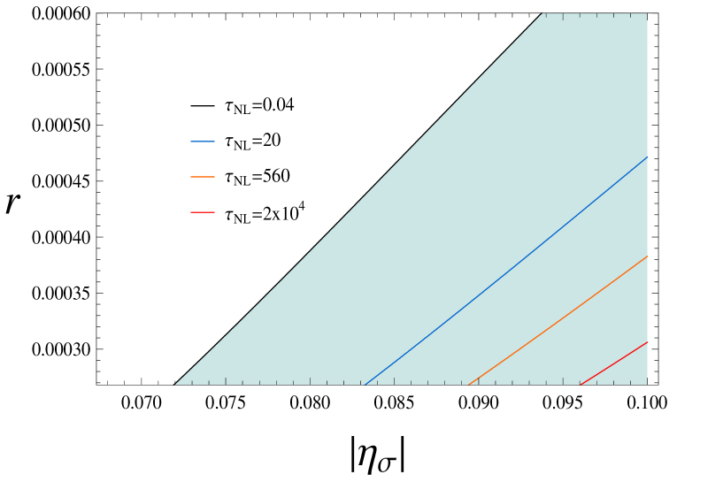
Figure 4.1: Contours of $\tau_{NL}$ in the $r$ vs $|\eta_{\sigma}|$ plot. The intermediate (high) $\phi_{\star}$ $T$-region corresponds to the shaded (white) region. The observationally expected $2\sigma$ range of values, for WMAP, PLANCK, and even the 21 cm background anisotropies, and for positive $\tau_{NL}$, $\tau_{NL}>20$ are completely inside the intermediate $\phi_{\star}$ $T$-region. Notice that the boundary line between the high and the intermediate $\phi_{\star}$ $T$-regions matches almost exactly the $\tau_{NL}=0.04$ line.

Now, by implementing the spectral tilt constraint in Eq. (3.52) in the spectrum normalisation constraint in Eq. (3.44) and the amount of inflation constraint in Eq. (3.58), we conclude that the tensor to scalar ratio $r$ is bounded from below: $r\mbox{\raisebox{-2.71246pt}{~{}$\stackrel{{\scriptstyle\mbox{$>$}}}{{\sim}}$~{}}}2.680\times 10^{-4}$.

In the $r$ vs $|\eta_{\sigma}|$ plot in figure 4.1, we show lines of constant $\tau_{NL}$ corresponding to the values $\tau_{NL}=20,560,2\times 10^{4}$. We also show the high (in white) and intermediate (shaded) $\phi_{\star}$ $T$-regions in agreement with the constraint in Eq. (4.23):

$$\frac{r\mathcal{P}_{\zeta}}{8}\frac{\eta_{\sigma}^{2}}{\eta_{\phi}^{2}}\exp[4N(|\eta_{\sigma}|-|\eta_{\phi}|)]\ll\left(\frac{\phi_{\star}}{m_{P}}\right)^{2}\ll\frac{r\mathcal{P}_{\zeta}}{2}\frac{\eta_{\sigma}^{4}}{\eta_{\phi}^{4}}\exp[8N(|\eta_{\sigma}|-|\eta_{\phi}|)]\,,$$

$$\Rightarrow\;\;4.070\times 10^{4}\ll|\eta_{\sigma}|^{4}\exp[400\ln(5.657\times 10^{-2}r^{-1/2})(|\eta_{\sigma}|-0.020)]\ll 1.656\times 10^{17}\,.$$ (4.32)

As is evident from the plot, the observationally expected $2\sigma$ range of values for WMAP, $|\tau_{NL}|\mbox{\raisebox{-2.71246pt}{~{}$\stackrel{{\scriptstyle\mbox{$>$}}}{{\sim}}$~{}}}2\times 10^{4}$ [112], PLANCK, $|\tau_{NL}|\mbox{\raisebox{-2.71246pt}{~{}$\stackrel{{\scriptstyle\mbox{$>$}}}{{\sim}}$~{}}}560$ [112], and even the 21 cm background anisotropies, $|\tau_{NL}|\mbox{\raisebox{-2.71246pt}{~{}$\stackrel{{\scriptstyle\mbox{$>$}}}{{\sim}}$~{}}}20$ [45], and for positive $\tau_{NL}$, are completely inside the intermediate $\phi_{\star}$ $T$-region as required. Higher values for $\tau_{NL}$, up to $\tau_{NL}=1.7\times 10^{5}$ are consistent within our framework for the intermediate $\phi_{\star}$ $T$-region.

In subsection 3.6, we studied $f_{NL}$ for the case when $\zeta$ is generated during inflation, $B_{\zeta}$ is dominated by the one-loop correction, and $P_{\zeta}$ is dominated by the tree-level term. Fig. 3.2 shows the results found. The WMAP [159] (and also PLANCK [120]) observationally allowed $2\sigma$ range of values for negative $f_{NL}$, $-9<f_{NL}$, is completely inside the intermediate $\phi_{\star}$ region. Fig. 4.2 shows both Figs. 3.2 and 4.1 in the same plot. Incidentally, for the available parameter window, lines for constant $\tau_{NL}$ almost exactly matches lines for constant $f_{NL}$. Thus, it is possible to see that, according the observational status presented in the Section 2.4, non-gaussianity is more likely to be detected through the trispectrum than through the bispectrum, for the inflationary model studied in this chapter with concave downward potential, and from the WMAP, PLANCK, and even the 21 cm background anisotropies observations. Fig. 4.2 also shows some consistency relations between the values of $f_{NL}$ and $\tau_{NL}$ that will be useful at testing the inflationary model considered with concave downward potential against observations. For instance, if WMAP detected non-gaussianity through the trispectrum with $\tau_{NL}\geq 8\times 10^{4}$ at the $2\sigma$ level, the slow-roll inflationary model with concave downward potential considered in this chapter would be ruled out since the predicted $f_{NL}$ would be outside the current observational interval.

Similarly to the $f_{NL}$ case, it is interesting to see a slow-roll inflationary model with canonical kinetic terms where large, and observable, values for $\tau_{NL}$ may be obtained (in contrast to the expected $\tau_{NL}\sim\mathcal{O}(r)$ from the tree-level calculation [188, 192]). So we conclude that if $T_{\zeta}$ is dominated by the one- loop correction but $P_{\zeta}$ is dominated by the tree-level term, sizeable non-gaussianity is generated even if $\zeta$ is generated during inflation.

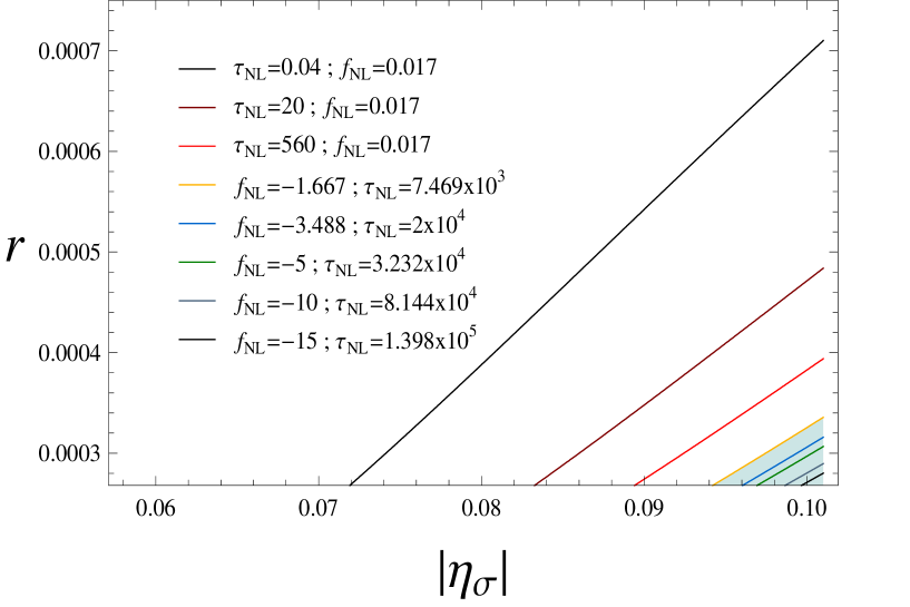
Figure 4.2: Contours of both $f_{NL}$ and $\tau_{NL}$ in the $r$ vs $|\eta_{\sigma}|$ plot. The intermediate (high) $\phi_{\star}$ region corresponds to the shaded (white) region. Lines for constant $\tau_{NL}$ almost exactly matches lines for constant $f_{NL}$. According to this figure, and to the observational status, non-gaussianity is more likely to be detected through the trispectrum than through the bispectrum, for the inflationary model studied in this chapter with concave downward potential, and from the WMAP, PLANCK, and even the 21 cm background anisotropies observations. These lines also show some consistency relations between the values of $f_{NL}$ and $\tau_{NL}$ that will be useful at testing the inflationary model considered with concave downward potential against observations.

4.6.2     The high $\phi_{\star}$ $T$-region

According to the expressions in Eqs. (2.35), (3.52), (4.6), (4.2) and (4.30) the value of $\tau_{NL}$ is in this case

$$\frac{1}{2}\tau_{NL}=\frac{T^{tree}_{\zeta}}{8\pi^{6}\left[\frac{1}{k_{2}^{3}k_{4}^{3}|{\bf k}_{3}+{\bf k}_{4}|^{3}}+23\;\;{\rm permutations}\right](\mathcal{P}^{tree}_{\zeta})^{3}}=\frac{1}{2}\eta_{\phi}^{2}=2\times 10^{-4}\,,$$ (4.33)

in agreement with the general expectations of Ref. [40] for slow-roll inflationary models with canonical kinetic terms where only the tree-level contributions are considered and the field perturbations are assumed to be gaussian. This result is no observational interest because the generated non-gaussianity is too small to be observable.

 SECTION 4.7      $\zeta$ not generated during inflation

We will assume in this Section that the fields driving inflation have nothing to do with the generation of $\zeta$; nevertheless, they will generate the primordial non-gaussianity (see for instance Refs. [31, 89, 104, 105, 106, 109, 126, 204]). To this end, the post-inflationary evolution, particularly the generation of $\zeta$, will be assumed not to generate significative levels of non-gaussianity in comparison with those generated during inflation.

4.7.1     $\tau_{\rm NL}$

The low $\phi_{\star}$ $T$-region

It is possible, in principle, that $P_{\zeta}$ is dominated by the one-loop correction as long as $\zeta$ is not generated during inflation. Thus, the observed spectral index constraint is no longer required and, therefore, the low $\phi_{\star}$ $T$-region is in principle viable.

Combining the conditions in Eqs. (4.20) and (4.28) with the expression for the number of e-folds in Eq. (3.57), we get:

$$1\mbox{\raisebox{-2.71246pt}{~{}$\stackrel{{\scriptstyle\mbox{$<$}}}{{\sim}}$~{}}}\frac{rn^{2}}{16}{\mathcal{P}}_{\zeta}\exp[N|\eta_{\sigma}|(4-2/n)]\,,$$ (4.34)

and

$$1\mbox{\raisebox{-2.71246pt}{~{}$\stackrel{{\scriptstyle\mbox{$>$}}}{{\sim}}$~{}}}10^{6}\left(\frac{rn}{16}\right)^{2}{\mathcal{P}}_{\zeta}\exp(4N|\eta_{\sigma}|)\,,$$ (4.35)

where we have defined the parameter $n$ as the ratio between the two $\eta$ parameters: $n=\eta_{\sigma}/\eta_{\phi}$. These two expressions lead to

$$rn\mbox{\raisebox{-2.71246pt}{~{}$\stackrel{{\scriptstyle\mbox{$<$}}}{{\sim}}$~{}}}1.6\times 10^{-5}|\eta_{\sigma}|\exp(-2N|\eta_{\sigma}|/n)\,,$$ (4.36)

as a necessary but not sufficient condition to satisfy both Eqs. (4.34) and (4.35). However, by introducing such a condition in Eq. (4.34), we see that the latter translate into the following constraint:

$$1\mbox{\raisebox{-2.71246pt}{~{}$\stackrel{{\scriptstyle\mbox{$<$}}}{{\sim}}$~{}}}10^{-6}|\eta_{\sigma}|^{2}{\mathcal{P}}_{\zeta}\exp[4N|\eta_{\sigma}|(1-1/n)]\,.$$ (4.37)

The previous expression is impossible to satisfy because the highest value the right hand side may take is for $n\rightarrow\infty$ and, of course, $\eta_{\sigma}=0.1$ and $N=62$. Such a value, $1.45\times 10^{-6}$, is much less than one. We conclude that this case is of no interest because it is imposible to satisfy the normalisation spectrum condition in Eq. (4.28).

The intermediate $\phi_{\star}$ $T$-region

The level of non-gaussianity $\tau_{NL}$ in this case is given by

$$\frac{1}{2}\tau_{NL} = \frac{T_{\zeta}^{1-loop}}{8\pi^{6}\left[\frac{1}{k_{2}^{3}k_{4}^{3}|{\bf k}_{3}+{\bf k}_{4}|^{3}}+23\;\;{\rm permutations}\right]{\mathcal{P}_{\zeta}^{3}}}$$ (4.38)

$$= \frac{2\eta_{\sigma}^{4}}{\eta_{\phi}^{8}\phi_{\star}^{8}}\exp[8N(|\eta_{\sigma}|-|\eta_{\phi}|)]\left(\frac{H_{\star}}{2\pi}\right){\mathcal{P}}_{\zeta}^{-3}\ln(kL)$$

$$= \frac{2\eta_{\sigma}^{4}}{\eta_{\phi}^{8}}\exp[8N(|\eta_{\sigma}|-|\eta_{\phi}|)]\left(\frac{m_{P}}{\phi_{\star}}\right)^{8}\left(\frac{r}{8}\right)^{4}{\mathcal{P}}_{\zeta}\ln(kL)$$

$$= \frac{2\eta_{\sigma}^{4}}{\eta_{\phi}^{4}}\left(\frac{1}{2\times 10^{-2}}\right)^{4}\exp(8N|\eta_{\sigma}|)\left(\frac{r}{8}\right)^{4}{\mathcal{P}}_{\zeta}\ln(kL)$$

$$\simeq 2.60\times 10^{16}\ (nr)^{4}\,,$$

where in the last line we have introduced again the ratio $n$ defined in previous subsubsection, and chosen for simplicity $|\eta_{\sigma}|=0.1$ and $N=62$ so that the non-gaussianity is maximized.

From Eqs. (4.23), (4.29) and (3.57), and those coming from the $\zeta$ series convergence constraints in Eqs. (3.76) and (3.77), with $|\eta_{\sigma}|=0.1$ and $N=62$, lead to the following conditions that reduce the available parameter space:

• The perturbative regime constraint $|x|\ll 1$:

  $$r\mbox{\raisebox{-2.71246pt}{~{}$\stackrel{{\scriptstyle\mbox{$<$}}}{{\sim}}$~{}}}6.51\times 10^{4}\ n\exp\left[-\frac{12.4}{n}\right]\,.$$ (4.39)

• The perturbative regime constraint $|y|\ll 1$:

  $$r\mbox{\raisebox{-2.71246pt}{~{}$\stackrel{{\scriptstyle\mbox{$<$}}}{{\sim}}$~{}}}\frac{2.68\times 10^{-1}}{n^{2}}\,.$$ (4.40)

• The $P_{\zeta}$ dominated by the tree-level term constraint:

  $$r\mbox{\raisebox{-2.71246pt}{~{}$\stackrel{{\scriptstyle\mbox{$<$}}}{{\sim}}$~{}}}\frac{1.10\times 10^{-4}}{n}\exp\left[\frac{12.4}{n}\right]\,.$$ (4.41)

• The $T_{\zeta}$ dominated by the one-loop correction constraint:

  $$r\mbox{\raisebox{-2.71246pt}{~{}$\stackrel{{\scriptstyle\mbox{$>$}}}{{\sim}}$~{}}}\frac{4.68\times 10^{-12}}{n^{3}}\exp\left[\frac{37.2}{n}\right]\,.$$ (4.42)

• The spectrum normalisation constraint:

  $$r\mbox{\raisebox{-2.71246pt}{~{}$\stackrel{{\scriptstyle\mbox{$<$}}}{{\sim}}$~{}}}\frac{1.6\times 10^{-4}}{n}\exp\left[-\frac{12.4}{n}\right]\,.$$ (4.43)

Analysing these expressions, we conclude that the constraint in the first item is automatically satisfied once the constraint in the fifth item is satisfied. Moreover, from the constraint in the fifth item, we see that the highest possible value $r$ may take is $4.75\times 10^{-6}$. And finally, to make the constraint in the fourth item consistent with the constraints in the second, third, and fifth items, the lower bound $n\mbox{\raisebox{-2.71246pt}{~{}$\stackrel{{\scriptstyle\mbox{$>$}}}{{\sim}}$~{}}}2.58$ is required. The resultant available parameter window, together with the lines for constant values of $\tau_{NL}$, $\tau_{NL}=1,5,10,15$, is presented in Fig. 4.3 for $2.58\leq n\leq 200$. Fig. 4.4 shows the range $200\leq n\leq 2000$ with the lines $\tau_{NL}=1,5$, while Fig. 4.5 shows the range $2000\leq n\leq 3000$ also with the lines $\tau_{NL}=1,5$. As the figures reveal, when $T_{\zeta}$ is dominated by the one-loop correction and $P_{\zeta}$ is dominated by the tree-level term, large values for $\tau_{NL}$ are obtained although not so large as in the case where $\zeta$ is generated during inflation. Indeed, an upper bound on $\tau_{NL}$, according to Eqs. (4.38) and (4.43), is $34.078$ when $n\rightarrow\infty$.

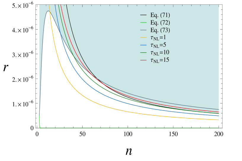
Figure 4.3: Contours of $\tau_{NL}$ in the $r$ vs $n$ plot, for $2.58\leq n\leq 200$, when $\zeta$ is not generated during inflation. The allowed parameter space corresponds to the white region. The constraint in Eq. (4.42) almost matches (visually) the horizontal axis. The largest possible value $\tau_{NL}$ may take in this range is 15.

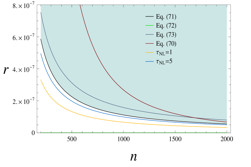
Figure 4.4: Contours of $\tau_{NL}$ in the $r$ vs $n$ plot, for $200\leq n\leq 2000$, when $\zeta$ is not generated during inflation. The allowed parameter space corresponds to the white region. The constraint in Eq. (4.42) matches (visually) the horizontal axis. The largest possible value $\tau_{NL}$ may take in this range is a bit higher than 5.

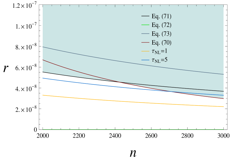
Figure 4.5: Contours of $\tau_{NL}$ in the $r$ vs $n$ plot, for $2000\leq n\leq 3000$, when $\zeta$ is not generated during inflation. The allowed parameter space corresponds to the white region. The constraint in Eq. (4.42) matches (visually) the horizontal axis. The largest possible value $\tau_{NL}$ may take in this range is a bit higher than 5.

We conclude that, even if $\zeta$ is not generated during inflation, we may find observable values for $\tau_{NL}$. However, such observable values could only be observed by the 21 cm background anisotropies at the $1\sigma$ level according to the observational status presented in Section 2.4. We also conclude that, for non- gaussianity to be observable, primordial gravitational waves must be undetectable.

The high $\phi_{\star}$ $T$-region

This case is of no interest because the generated non-gaussianity is too small to be observable:

$$\frac{1}{2}\tau_{NL} = \frac{T_{\zeta}^{tree}}{8\pi^{6}\left[\frac{1}{k_{2}^{3}k_{4}^{3}|{\bf k}_{3}+{\bf k}_{4}|^{3}}+23\;\;{\rm permutations}\right]{\mathcal{P}_{\zeta}^{3}}}$$ (4.44)

$$= \frac{T_{\zeta}^{tree}}{8\pi^{6}\left[\frac{1}{k_{2}^{3}k_{4}^{3}|{\bf k}_{3}+{\bf k}_{4}|^{3}}+23\;\;{\rm permutations}\right]\left(\mathcal{P}_{\zeta}^{tree}\right)^{3}}\frac{\left(\mathcal{P}_{\zeta}^{tree}\right)^{3}}{\mathcal{P}_{\zeta}^{3}}\;=\;\frac{1}{2}|\eta_{\phi}|^{2}\frac{\left(\mathcal{P}_{\zeta}^{tree}\right)^{3}}{\mathcal{P}_{\zeta}^{3}}$$

$$\Rightarrow \tau_{NL}\;\ll\;|\eta_{\phi}|^{2}\,,$$

according to the expressions in Eqs. (4.2) and (4.6).

4.7.2     $f_{NL}$

The low $\phi_{\star}$ region

From Eqs. (3.34) and (4.20) we see that the low $\phi_{\star}$ region and the low $\phi_{\star}$ $T$-region are exactly the same, being only constrained by the fact that $P_{\zeta}$ is dominated by the one-loop correction. Thus, the obtained conclusions in Subsubsection 4.7.1 equally apply. Therefore, this case is of no interest because it is impossible to satisfy the normalisation spectrum condition in Eq. (4.28) for the low $\phi_{\star}$ region.

The intermediate $\phi_{\star}$ region

The level of non-gaussianity is in this case given by

$$\frac{6}{5}f_{NL} = \frac{B_{\zeta}^{1-loop}}{4\pi^{4}\frac{\sum_{i}k_{i}^{3}}{\prod_{i}k_{i}^{3}}\mathcal{P}_{\zeta}^{2}}=\frac{\eta_{\sigma}^{3}}{\eta_{\phi}^{6}\phi_{\star}^{6}}\exp[6N(|\eta_{\sigma}|-|\eta_{\phi}|)]\left(\frac{H_{\star}}{2\pi}\right)^{6}\mathcal{P}_{\zeta}^{-2}\ln(kL)$$ (4.45)

$$= \frac{\eta_{\sigma}^{3}}{\eta_{\phi}^{6}}\exp[6N(|\eta_{\sigma}|-|\eta_{\phi}|)]\left(\frac{m_{P}}{\phi_{\star}}\right)^{6}\left(\frac{r}{8}\right)^{3}\mathcal{P}_{\zeta}\ln(kL)$$

$$= -\frac{\eta_{\sigma}^{3}}{\eta_{\phi}^{3}}\left(\frac{1}{2\times 10^{-2}}\right)^{3}\exp(6N|\eta_{\sigma}|)\left(\frac{r}{8}\right)^{3}\mathcal{P}_{\zeta}\ln(kL)$$

$$\approx -8.59\times 10^{9}(nr)^{3}\,,$$

where in the last line we have chosen again for simplicity $|\eta_{\sigma}|=0.1$ and $N=62$ so that the non-gaussianity is maximized.

Since the spectrum normalisation constraint in Eq. (4.43) equally applies to this case, we conclude from it and from Eq. (4.45) that an upper bound on $|f_{NL}|$ is $2.93\times 10^{-2}$ when $n\rightarrow\infty$. $f_{NL}$ is, of course, unobservable. We conclude that when $\zeta$ is not generated during inflation, but the primordial non- gaussianity is, it is impossible to detect non-gaussianity through the bispectrum. However, in view of Subsubsection 4.7.1, it is possible to detect it through the trispectrum.

The high $\phi_{\star}$ region

This case is of no interest because the generated non-gaussianity is too small to be observable:

$$\frac{6}{5}f_{NL}=\frac{B_{\zeta}^{tree}}{4\pi^{4}\frac{\sum_{i}k_{i}^{3}}{\prod_{i}k_{i}^{3}}\mathcal{P}_{\zeta}^{2}}=\frac{B_{\zeta}^{tree}}{4\pi^{4}\frac{\sum_{i}k_{i}^{3}}{\prod_{i}k_{i}^{3}}\left(\mathcal{P}_{\zeta}^{tree}\right)^{2}}\frac{\left(\mathcal{P}_{\zeta}^{tree}\right)^{2}}{\mathcal{P}_{\zeta}^{2}}=|\eta_{\phi}|\frac{\left(\mathcal{P}_{\zeta}^{tree}\right)^{2}}{\mathcal{P}_{\zeta}^{2}}\ll|\eta_{\phi}|\,,$$ (4.46)

according to the expressions in Eqs. (3.27) and (3.29).

 SECTION 4.8      Conclusions

In this chapter we extended the analysis given in the previous one, but this time we calculated the trispectrum $T_{\zeta}$ of the primordial curvature perturbation $\zeta$, generated during a slow-roll inflationary epoch and considering a two- field quadratic model of inflation with canonical kinetic terms. In order to obtain a large level of non-gaussianity, we consider loop contributions as well as tree level terms, and show that it is possible to attain very high, including observable, values for the level of non-gaussianity $\tau_{NL}$ if $T_{\zeta}$ is dominated by the one-loop contribution and $P_{\zeta}$ is dominated by tree level term. The statement presented in Ref. [38] about the suppression of the loop corrections against the tree-level terms when considering classicality was analyzed in this chapter and argued to be too strongly stated leading to non-general conclusions. The probability that a typical observer sees a non-gaussian distribution in the model considered in this thesis was investigated and found to be non-negligible.

Chapter 5          NON-GAUSSIANITY FROM VECTOR FIELD PERTURBATIONS

 SECTION 5.1      Introduction

The anisotropies in the temperature of the cosmic microwave background (CMB) radiation, which have strong connections with the origin of the large-scale structure in the observable Universe, is one of hottest topics in modern cosmology. The properties of the CMB temperature anisotropies are described in terms of the spectral functions, like the spectrum, bispectrum, trispectrum, etc., of the primordial curvature perturbation $\zeta$ [43]. In most of the cosmological models the $n$-point correlators of $\zeta$ are supposed to be translationally and rotationally invariants. However, violations of such invariances entail modifications of the usual definitions for the spectral functions in terms of the statistical descriptors [1, 12, 41]. These violations may be consequences either of the presence of vector field perturbations [12, 19, 49, 50, 51, 52, 53, 54, 73, 74, 75, 76, 94, 95, 96, 97, 102, 103, 113, 224], spinor field perturbations [30, 194], or p-form perturbations [70, 71, 111, 115, 116], contributing significantly to $\zeta$, of anisotropic expansion [17, 30, 47, 81, 97, 102, 115, 165, 166, 218] or of an inhomogeneous background [12, 41, 52]. Violation of the statistical isotropy (i.e. violation of the rotational invariance in the $n$-point correlators of $\zeta$) seems to be present in the data [14, 80, 88, 178] and, although its statistical significance is still low, the continuous presence of anomalies in every CMB data analysis (see for instance Refs. [34, 58, 62, 63, 85, 86, 91, 92, 122, 123, 162, 184, 205]) suggests the evidence might be decisive in the forthcoming years. Since the statistical anisotropy is observationally low, it entails a big problem when vector fields are present during inflation, because they generically lead to a high amount of statistical anisotropy, higher than that coming from observations [52, 75, 102]. To solve this problem, people use different mechanisms in order to make those models consistent with observation, for example using a triad of orthogonal vectors [12, 25], a large number of identical randomly oriented vectors fields [75], or assuming that the contribution of vector fields to the total energy density is negligible [52, 102].

The amount of statistical anisotropy is quantified throught the parameter $g_{\zeta}$, usually called the level of statistical anisotropy in the spectrum. Eq. (2.34) gives us the primordial power spectrum that takes into account the leading effects of violations of statistical isotropy by the presence of some vector field in the inflationary era. As we could see in Section 2.4 the $g_{\zeta}$ parameter has observational bounds and works, together with the non-gaussianity parameters $f_{\rm NL}$, $\tau_{\rm NL}$, $g_{\rm NL}$, etc., as statistical descriptors for $\zeta$. Therefore, it could be a crucial tool to discriminate between some of the more usual cosmological models.

Recent works point out the possibility that a vector field causes part of the primordial curvature perturbation and show that the particular presence of vector fields in the inflationary dynamics may generate sizeable levels of non-gaussianity described by $f_{\rm NL}$ [23, 103, 210] and $\tau_{\rm NL}$ [20, 209]. In such works the authors included both vector and scalar field perturbations, and asummed that the contributions to the spectrum from vector field perturbations were smaller than those coming from scalar fields and in an opposite way for bispectrum and trispectrum.

In this chapter we use the $\delta N$ formalism to calculate the tree-level and one-loop contributions to the bispectrum $B_{\zeta}$ and trispectrum $T_{\zeta}$ of $\zeta$, including vector and scalar field perturbations. We then calculate the order of magnitude of the levels of non-gaussianity in $B_{\zeta}$ and $T_{\zeta}$ including the one-loop contributions and write down formulas that relate the order of magnitude of the levels of non-gaussianity $f_{\rm NL}$ and $\tau_{\rm NL}$ with the amount of statistical anisotropy in the spectrum $g_{\zeta}$. Finally, comparison with the expected observational bound from WMAP is done.

 SECTION 5.2      Statistical descriptors from vector field perturbations

As we saw in Chapter 2, the $\delta N$ formalism [52, 139, 142, 182, 202, 181] is a powerful tool to calculate the primordial curvature perturbation and all its statistical descriptor to any desired order. In the simplest case where $\zeta$ is generated by one scalar field and one vector field and assuming that the anisotropy in the expansion of the Universe is negligible, it can be calculated up to quadratic terms by means of the following truncated expansion [52]:

$$\zeta({\mathbf{x}})\equiv\delta N(\phi({\mathbf{x}}),A_{i}({\mathbf{x}}),t)=N_{\phi}\delta\phi+N_{A}^{i}\delta A_{i}+\frac{1}{2}N_{\phi\phi}(\delta\phi)^{2}+N_{\phi A}^{i}\delta\phi\delta A_{i}+\frac{1}{2}N_{AA}^{ij}\delta A_{i}\delta A_{j}\,,$$ (5.1)

where

$$N_{\phi}\equiv\frac{\partial N}{\partial\phi}\,,\quad N_{A}^{i}\equiv\frac{\partial N}{\partial A_{i}}\,,\quad N_{\phi\phi}\equiv\frac{\partial^{2}N}{\partial\phi^{2}}\,,\quad N_{AA}^{ij}\equiv\frac{\partial^{2}N}{\partial A_{i}\partial A_{j}}\,,\quad N_{\phi A}^{i}\equiv\frac{\partial^{2}N}{\partial A_{i}\partial\phi}\,,$$ (5.2)

$\phi$ being the scalar field and ${\bf A}$ the vector field, with $i$ denoting the spatial indices running from 1 to 3. In the Section 2.3 we defined the power spectrum $P_{\zeta}$, the bispectrum $B_{\zeta}$ and trispectrum $T_{\zeta}$ for the primordial curvature perturbation, through the Fourier modes of $\zeta$ as:

$$\langle\zeta({\mathbf{k}})\zeta({\mathbf{k}}^{\prime})\rangle \equiv (2\pi)^{3}\delta({\mathbf{k}}+{\mathbf{k}}^{\prime})P_{\zeta}({\mathbf{k}})\;\;\equiv\;\;(2\pi)^{3}\delta({\mathbf{k}}+{\mathbf{k}}^{\prime})\frac{2\pi^{2}}{k^{3}}{{\cal P}_{\zeta}}({\mathbf{k}})\,,$$ (5.3)

$$\langle\zeta({\mathbf{k}})\zeta({\mathbf{k}}^{\prime})\zeta({\mathbf{k}}^{\prime\prime})\rangle \equiv (2\pi)^{3}\delta({\mathbf{k}}+{\mathbf{k}}^{\prime}+{\mathbf{k}}^{\prime\prime})B_{\zeta}({\mathbf{k}},{\mathbf{k}}^{\prime},{\mathbf{k}}^{\prime\prime})\;\;$$ (5.4)

$$\equiv \;\;(2\pi)^{3}\delta({\mathbf{k}}+{\mathbf{k}}^{\prime}+{\mathbf{k}}^{\prime\prime})\frac{4\pi^{4}}{k^{3}k^{\prime 3}}{{\cal B}_{\zeta}}({\mathbf{k}},{\mathbf{k}}^{\prime},{\mathbf{k}}^{\prime\prime})\,.$$

$$\langle\zeta({\mathbf{k}}_{1})\zeta({\mathbf{k}}_{2})\zeta({\mathbf{k}}_{3})\zeta({\mathbf{k}}_{4})\rangle \equiv (2\pi)^{4}\delta({\mathbf{k}}_{1}+{\mathbf{k}}_{2}+{\mathbf{k}}_{3}+{\mathbf{k}}_{4})T_{\zeta}({\mathbf{k}}_{1},{\mathbf{k}}_{2},{\mathbf{k}}_{3},{\mathbf{k}}_{4})$$ (5.5)

$$\equiv (2\pi)^{3}\delta({\mathbf{k}}_{1}+{\mathbf{k}}_{2}+{\mathbf{k}}_{3}+{\mathbf{k}}_{4})\frac{\left(2\pi^{2}\right)^{3}}{k_{1}^{3}k_{2}^{3}|{\mathbf{k}}_{2}+{\mathbf{k}}_{3}|^{3}}{{\cal T}_{\zeta}}({\mathbf{k}}_{1},{\mathbf{k}}_{2},{\mathbf{k}}_{3},{\mathbf{k}}_{4})\,.$$

Using Eq. (5.1) and the definitions given in Eqs. (5.3) and (5.4), it was found in Ref. [52] that the tree-level contribution to the spectrum is of the form shown in Eq. (2.36), that is

$$P_{\zeta}({\mathbf{k}})=P_{\zeta}^{\rm iso}(k)\left(1+g_{\zeta}(\hat{{\mathbf{d}}}\cdot\hat{\mathbf{k}})^{2}\right)\,.$$ (5.6)

In addition, an analogous form for the contribution to $f_{\rm NL}$ was given in Ref. [103], showing that both, $P_{\zeta}$ and $f_{\rm NL}$ have anisotropic contributions coming from the vector field perturbation. The one-loop correction to the spectrum was also given in Ref. [52], however they kept it in an integral form. In this chapter we give the tree-level and one-loop contributions to the bispectrum and to the trispectrum. We also estimate the integrals coming from loop corections in order to get an order of magnitude for $f_{\rm NL}$ and $\tau_{\rm NL}$.

Using the Fourier fmodes for Eqs. Eq. (5.1), (5.3), (5.4) and (5.5) and considering contributions up to one-loop order, the expressions for ${{\cal P}_{\zeta}}$, ${{\cal B}_{\zeta}}$ and ${{\cal T}_{\zeta}}$ , are:

$${\cal P}_{\zeta}^{\rm tree}({\mathbf{k}}) = N_{\phi}^{2}{\cal P}_{\delta\phi}(k)+N_{A}^{i}N_{A}^{j}{\cal T}_{ij}({\mathbf{k}})$$ (5.7)

$$= N_{\phi}^{2}{\cal P}_{\delta\phi}(k)+N_{A}^{2}{\cal P}_{+}(k)+({\bf N}_{A}\cdot\hat{\mathbf{k}})^{2}{\cal P}_{+}(k)\left(r_{\rm long}-1\right)\,,$$

$${\cal P}_{\zeta}^{\rm 1-loop}({\mathbf{k}}) = \int\frac{d^{3}pk^{3}}{4\pi|{\mathbf{k}}+{\mathbf{p}}|^{3}p^{3}}\left[\frac{1}{2}N_{\phi\phi}^{2}{\cal P}_{\delta\phi}(|{\mathbf{k}}+{\mathbf{p}}|){\cal P}_{\delta\phi}(p)+N_{\phi A}^{i}N_{\phi A}^{j}{\cal P}_{\delta\phi}(|{\mathbf{k}}+{\mathbf{p}}|){\cal T}_{ij}({\mathbf{p}})\right.$$ (5.8)

$$\left.+\frac{1}{2}N_{AA}^{ij}N_{AA}^{kl}{\cal T}_{ik}({\mathbf{k}}+{\mathbf{p}}){\cal T}_{jl}({\mathbf{p}})\right]\,,$$

$${\cal B}_{\zeta}^{\rm tree}({\mathbf{k}},{\mathbf{k}}^{\prime},{\mathbf{k}}^{\prime\prime}) = N_{\phi}^{2}N_{\phi\phi}[{\cal P}_{\delta\phi}(k){\cal P}_{\delta\phi}(k^{\prime})+{\rm c.\ p.}]+N_{A}^{i}N_{A}^{k}N_{AA}^{mn}\Big{[}{\cal T}_{im}({\mathbf{k}}){\cal T}_{kn}({\mathbf{k}}^{\prime})+{\rm c.\ p.}\Big{]}$$ (5.9)

$$+ N_{\phi}N_{A}^{i}N_{\phi A}^{j}\Big{[}{\cal P}_{\delta\phi}(k){\cal T}_{ij}({\mathbf{k}}^{\prime})+5\ {\rm perm.}\Big{]}\,,$$

$${\cal B}_{\zeta}^{\rm 1-loop}({\mathbf{k}},{\mathbf{k}}^{\prime},{\mathbf{k}}^{\prime\prime}) = N_{\phi\phi}^{6}\int\frac{d^{3}pk^{3}k^{\prime 3}}{4\pi p^{3}|{\mathbf{k}}+{\mathbf{p}}|^{3}|{\mathbf{k}}^{\prime}-{\mathbf{p}}|^{3}}{\cal P}_{\delta\phi}(p){\cal P}_{\delta\phi}(|{\mathbf{k}}+{\mathbf{p}}|){\cal P}_{\delta\phi}(|{\mathbf{k}}^{\prime}-{\mathbf{p}}|)$$ (5.10)

$$+ N_{AA}^{ij}N_{AA}^{kl}N_{AA}^{mn}\int\frac{d^{3}pk^{3}k^{\prime 3}}{4\pi p^{3}|{\mathbf{k}}+{\mathbf{p}}|^{3}|{\mathbf{k}}^{\prime}-{\mathbf{p}}|^{3}}{\cal T}_{il}({\mathbf{p}}){\cal T}_{kn}({\mathbf{k}}+{\mathbf{p}}){\cal T}_{jm}({\mathbf{k}}^{\prime\prime}-{\mathbf{p}})$$

$$+ N_{\phi\phi}N_{\phi A}^{i}N_{\phi A}^{j}\int\frac{d^{3}pk^{3}k^{\prime 3}}{4\pi p^{3}|{\mathbf{k}}^{\prime\prime}+{\mathbf{p}}|^{3}|{\mathbf{k}}^{\prime}-{\mathbf{p}}|^{3}}\bigg{\{}{\cal P}_{\delta\phi}(p){\cal P}_{\delta\phi}(|{\mathbf{k}}^{\prime\prime}+{\mathbf{p}}|){\cal T}_{ij}({\mathbf{k}}^{\prime}-{\mathbf{p}})$$

$$+ {\cal P}_{\delta\phi}(p){\cal P}_{\delta\phi}(|{\mathbf{k}}^{\prime}-{\mathbf{p}}|){\cal T}_{ij}({\mathbf{k}}^{\prime\prime}+{\mathbf{p}})+{\cal P}_{\delta\phi}(|{\mathbf{k}}^{\prime}-{\mathbf{p}}|){\cal P}_{\delta\phi}(|{\mathbf{k}}^{\prime\prime}+{\mathbf{p}}|){\cal T}_{ij}({\mathbf{p}})\bigg{\}}$$

$$+ N_{\phi A}^{i}N_{\phi A}^{j}N_{AA}^{kl}\int\frac{d^{3}pk^{3}k^{\prime 3}}{4\pi p^{3}|{\mathbf{k}}^{\prime\prime}+{\mathbf{p}}|^{3}|{\mathbf{k}}^{\prime}-{\mathbf{p}}|^{3}}\bigg{\{}{\cal P}_{\delta\phi}(p){\cal T}_{ik}({\mathbf{k}}^{\prime}-{\mathbf{p}}){\cal T}_{jl}({\mathbf{k}}^{\prime\prime}+{\mathbf{p}})$$

$$+ {\cal P}_{\delta\phi}(|{\mathbf{k}}^{\prime\prime}+{\mathbf{p}}|){\cal T}_{ik}({\mathbf{p}}){\cal T}_{jl}({\mathbf{k}}^{\prime}-{\mathbf{p}})+{\cal P}_{\delta\phi}(|{\mathbf{k}}^{\prime}-{\mathbf{p}}|){\cal T}_{ik}({\mathbf{p}}){\cal T}_{jl}({\mathbf{k}}^{\prime\prime}+{\mathbf{p}})\bigg{\}}\,,$$

$${\cal T}_{\zeta}^{\rm tree}({\mathbf{k}}_{1},{\mathbf{k}}_{2},{\mathbf{k}}_{3},{\mathbf{k}}_{4}) = N_{\phi}^{2}N_{\phi\phi}^{2}[{\cal P}_{\delta\phi}(k_{2}){\cal P}_{\delta\phi}(k_{4}){\cal P}_{\delta\phi}(|{\mathbf{k}}_{1}+{\mathbf{k}}_{2}|)+{\rm 11\ perm.}]$$ (5.11)

$$+ N_{A}^{i}N_{A}^{j}N_{AA}^{kl}N_{AA}^{mn}\Big{[}{\cal T}_{ik}({\mathbf{k}}_{2}){\cal T}_{jm}({\mathbf{k}}_{4}){\cal T}_{ln}({\mathbf{k}}_{1}+{\mathbf{k}}_{2})+{\rm 11\ perm.}\Big{]}$$

$$+ N_{\phi}^{2}N_{A\phi}^{i}N_{A\phi}^{j}\Big{[}{\cal P}_{\delta\phi}(k_{2}){\cal P}_{\delta\phi}(k_{4}){\cal T}_{ij}({\mathbf{k}}_{1}+{\mathbf{k}}_{2})+11\ {\rm perm.}\Big{]}$$

$$+ N_{A}^{i}N_{A}^{j}N_{A\phi}^{k}N_{A\phi}^{l}\Big{[}{\cal T}_{ik}({\mathbf{k}}_{2}){\cal T}_{jl}({\mathbf{k}}_{4}){\cal P}_{\delta\phi}(|{\mathbf{k}}_{1}+{\mathbf{k}}_{2}|)+11\ {\rm perm.}\Big{]}$$

$$+ N_{\phi}N_{\phi\phi}N_{A}^{i}N_{A\phi}^{j}\Big{[}{\cal P}_{\delta\phi}(k_{2}){\cal T}_{ij}({\mathbf{k}}_{4}){\cal P}_{\delta\phi}(|{\mathbf{k}}_{1}+{\mathbf{k}}_{2}|)+23\ {\rm perm.}\Big{]}$$

$$+ N_{\phi}N_{A}^{i}N_{A\phi}^{j}N_{AA}^{kl}\Big{[}{\cal P}_{\delta\phi}(k_{2}){\cal T}_{ik}({\mathbf{k}}_{4}){\cal T}_{jl}({\mathbf{k}}_{1}+{\mathbf{k}}_{2})+23\ {\rm perm.}\Big{]}\,,$$

$${\cal T}_{\zeta A}^{\rm 1-loop}({\mathbf{k}}_{1},{\mathbf{k}}_{2},{\mathbf{k}}_{3},{\mathbf{k}}_{4}) = N_{AA}^{ij}N_{AA}^{kl}N_{AA}^{mn}N_{AA}^{op}\int\frac{d^{3}p\ k_{1}^{3}k_{3}^{3}|{\mathbf{k}}_{3}+{\mathbf{k}}_{4}|^{3}}{4\pi p^{3}|{\mathbf{k}}_{1}-{\mathbf{p}}|^{3}|{\mathbf{k}}_{3}+{\mathbf{p}}|^{3}|{\mathbf{k}}_{3}+{\mathbf{k}}_{4}+{\mathbf{p}}|^{3}}\times$$ (5.12)

$$\times{\cal T}_{im}({\mathbf{p}}){\cal T}_{jk}({\mathbf{k}}_{1}-{\mathbf{p}}){\cal T}_{np}({\mathbf{k}}_{3}+{\mathbf{p}}){\cal T}_{lo}({\mathbf{k}}_{3}+{\mathbf{k}}_{4}+{\mathbf{p}})\,,$$

where

$${\cal T}_{ij}({\mathbf{k}})\equiv T_{ij}^{\rm even}({\mathbf{k}}){\cal P}_{+}(k)+iT_{ij}^{\rm odd}({\mathbf{k}}){\cal P}_{-}(k)+T^{\rm long}_{ij}({\mathbf{k}}){\cal P}_{\rm long}(k)\,,$$ (5.13)

and

$$T_{ij}^{\rm even}({\mathbf{k}})\equiv\delta_{ij}-\hat{k}_{i}\hat{k}_{j}\,,\qquad T^{\rm odd}_{ij}({\mathbf{k}})\equiv\epsilon_{ijk}\hat{k}_{k}\,,\qquad T^{\rm long}_{ij}({\mathbf{k}})\equiv\hat{k}_{i}\hat{k}_{j}\,.$$ (5.14)

Eq. (5.7) was writen in the form of Eq. (5.6) with $\hat{{\mathbf{d}}}=\hat{{\mathbf{N}}}_{A}$, ${\mathbf{N}}_{A}$ being a vector with magnitude $N_{A}\equiv\sqrt{N^{i}_{A}N^{i}_{A}}$, and $r_{\rm long}\equiv{\cal P}_{\rm long}/{\cal P}_{+}$, where ${\cal P}_{\rm long}$ is the power spectrum for the longitudinal component, and ${\cal P}_{+}$ and ${\cal P}_{-}$ are the parity conserving and violating power spectra defined by

$${\cal P}_{\pm}\equiv\frac{1}{2}\left({\cal P}_{R}\pm{\cal P}_{L}\right)\,,$$ (5.15)

with ${\cal P}_{R}$ and ${\cal P}_{L}$ denoting the power spectra for the transverse components with right-handed and left-handed polarisations [52].

The above expressions can be further separated into different terms: one due to perturbations in the scalar field, another due to the vector field perturbations, and the other due to the mixed terms:

$${{\cal P}_{\zeta}}^{\rm tree}({\mathbf{k}}) = {{\cal P}_{\zeta}}_{\phi}^{\rm tree}(k)+{{\cal P}_{\zeta}}_{A}^{\rm tree}({\mathbf{k}}),$$ (5.16)

$${\cal P}_{\zeta}^{\rm 1-loop}({\mathbf{k}}) = {{\cal P}_{\zeta}}_{\phi}^{\rm 1-loop}(k)+{{\cal P}_{\zeta}}_{A}^{\rm 1-loop}({\mathbf{k}})+{{\cal P}_{\zeta}}_{\phi A}^{\rm 1-loop}({\mathbf{k}})\,,$$ (5.17)

$${\cal B}_{\zeta}^{\rm tree}({\mathbf{k}},{\mathbf{k}}^{\prime},{\mathbf{k}}^{\prime\prime}) = {{\cal B}_{\zeta}}_{\phi}^{\rm tree}({\mathbf{k}},{\mathbf{k}}^{\prime},{\mathbf{k}}^{\prime\prime})+{{\cal B}_{\zeta}}_{A}^{\rm tree}({\mathbf{k}},{\mathbf{k}}^{\prime},{\mathbf{k}}^{\prime\prime})+{{\cal B}_{\zeta}}_{\phi A}^{\rm tree}({\mathbf{k}},{\mathbf{k}}^{\prime},{\mathbf{k}}^{\prime\prime})\,,$$ (5.18)

$${\cal B}_{\zeta}^{\rm 1-loop}({\mathbf{k}},{\mathbf{k}}^{\prime},{\mathbf{k}}^{\prime\prime}) = {{\cal B}_{\zeta}}_{\phi}^{\rm 1-loop}({\mathbf{k}},{\mathbf{k}}^{\prime},{\mathbf{k}}^{\prime\prime})+{{\cal B}_{\zeta}}_{A}^{\rm 1-loop}({\mathbf{k}},{\mathbf{k}}^{\prime},{\mathbf{k}}^{\prime\prime})$$ (5.19)

$$+ {{\cal B}_{\zeta}}_{\phi A}^{\rm 1-loop}({\mathbf{k}},{\mathbf{k}}^{\prime},{\mathbf{k}}^{\prime\prime})\,,$$

$${\cal T}_{\zeta}^{\rm tree}({\mathbf{k}}_{1},{\mathbf{k}}_{2},{\mathbf{k}}_{3},{\mathbf{k}}_{4}) = {{\cal T}_{\zeta}}_{\phi}^{\rm tree}({\mathbf{k}}_{1},{\mathbf{k}}_{2},{\mathbf{k}}_{3},{\mathbf{k}}_{4})+{{\cal T}_{\zeta}}_{A}^{\rm tree}({\mathbf{k}}_{1},{\mathbf{k}}_{2},{\mathbf{k}}_{3},{\mathbf{k}}_{4})$$ (5.20)

$$+ {{\cal T}_{\zeta}}_{\phi A}^{\rm tree}({\mathbf{k}}_{1},{\mathbf{k}}_{2},{\mathbf{k}}_{3},{\mathbf{k}}_{4})\,,$$

$${\cal T}_{\zeta}^{\rm 1-loop}({\mathbf{k}}_{1},{\mathbf{k}}_{2},{\mathbf{k}}_{3},{\mathbf{k}}_{4}) = {{\cal T}_{\zeta}}_{\phi}^{\rm 1-loop}({\mathbf{k}}_{1},{\mathbf{k}}_{2},{\mathbf{k}}_{3},{\mathbf{k}}_{4})+{{\cal T}_{\zeta}}_{A}^{\rm 1-loop}({\mathbf{k}}_{1},{\mathbf{k}}_{2},{\mathbf{k}}_{3},{\mathbf{k}}_{4})$$ (5.21)

$$+ {{\cal T}_{\zeta}}_{\phi A}^{\rm 1-loop}({\mathbf{k}}_{1},{\mathbf{k}}_{2},{\mathbf{k}}_{3},{\mathbf{k}}_{4})\,,$$

Observational analysis tell us that the statistical anisotropy in CMB temperature perturbation could be observable in a future through current experiments like WMAP or PLANCK. Eq. (5.6) combined with recent studies [80] tells us that the level of statistical anisotropies $g_{\zeta}$ has an upper bound and in the best case ($99\%$ confidence level) this is $g_{\zeta}\mbox{\raisebox{-2.71246pt}{~{}$\stackrel{{\scriptstyle\mbox{$<$}}}{{\sim}}$~{}}}0.383$ [79]. During our analysis we will adopt an upper bound for $g_{\zeta}$: $g_{\zeta}\mbox{\raisebox{-2.71246pt}{~{}$\stackrel{{\scriptstyle\mbox{$<$}}}{{\sim}}$~{}}}0.1$. In order to satisfy the latter observational constraint over the spectrum, we must be sure that the contributions coming from vector fields in Eqs. (5.7) and (5.8) are smaller than those coming from scalar fields. That means that the first term in Eq. (5.16) dominates over all the other terms, even those coming from one-loop contributions. With the previous conclusion in mind we feel free to make assumptions over the other contributions, specially for those coming from vector field perturbations.

 SECTION 5.3      Vector field contributions to the statistical descriptors

As we explain in the previous section, our unique restriction from observation is related to the amount of statistical anisotropy present in the spectrum, so we need to be sure that the first term in Eq. (5.16) always dominates. In our study we will assume that the terms coming only from the vector field dominate over those coming from the mixed terms and from the scalar fields only, except for the case of the tree-level spectrum. Based on the assumption made, Eqs. (5.16) - (5.19) take the form:

$${{\cal P}_{\zeta}}^{\rm tree}({\mathbf{k}}) = {{\cal P}_{\zeta}}_{\phi}^{\rm tree}(k)+{{\cal P}_{\zeta}}_{A}^{\rm tree}({\mathbf{k}})\,,$$ (5.22)

$${\cal P}_{\zeta}^{\rm 1-loop}({\mathbf{k}}) = {{\cal P}_{\zeta}}_{A}^{\rm 1-loop}({\mathbf{k}})\,,$$ (5.23)

$${\cal B}_{\zeta}^{\rm tree}({\mathbf{k}},{\mathbf{k}}^{\prime},{\mathbf{k}}^{\prime\prime}) = {{\cal B}_{\zeta}}_{A}^{\rm tree}({\mathbf{k}},{\mathbf{k}}^{\prime},{\mathbf{k}}^{\prime\prime})\,,$$ (5.24)

$${\cal B}_{\zeta}^{\rm 1-loop}({\mathbf{k}},{\mathbf{k}}^{\prime},{\mathbf{k}}^{\prime\prime}) = {{\cal B}_{\zeta}}_{A}^{\rm 1-loop}({\mathbf{k}},{\mathbf{k}}^{\prime},{\mathbf{k}}^{\prime\prime})\,$$ (5.25)

$${\cal T}_{\zeta}^{\rm tree}({\mathbf{k}}_{1},{\mathbf{k}}_{2},{\mathbf{k}}_{3},{\mathbf{k}}_{4}) = {{\cal T}_{\zeta}}_{A}^{\rm tree}({\mathbf{k}}_{1},{\mathbf{k}}_{2},{\mathbf{k}}_{3},{\mathbf{k}}_{4})\,,$$ (5.26)

$${\cal T}_{\zeta}^{\rm 1-loop}({\mathbf{k}}_{1},{\mathbf{k}}_{2},{\mathbf{k}}_{3},{\mathbf{k}}_{4}) = {{\cal T}_{\zeta}}_{A}^{\rm 1-loop}({\mathbf{k}}_{1},{\mathbf{k}}_{2},{\mathbf{k}}_{3},{\mathbf{k}}_{4})\,,$$ (5.27)

The above expressions lead us to eight different ways that allow us to study and probably get a high level of non- gaussianity

• Vector field spectrum (${\cal P}_{\zeta_{A}}$) and bispectrum (${\cal B}_{\zeta_{A}}$) dominated by the tree-level terms [103].

• Vector field spectrum (${\cal P}_{\zeta_{A}}$) and bispectrum (${\cal B}_{\zeta_{A}}$) dominated by the 1-loop contributions.

• Vector field spectrum (${\cal P}_{\zeta_{A}}$) dominated by the tree-level terms and bispectrum (${\cal B}_{\zeta_{A}}$) dominated by the 1-loop contributions.

• Vector field spectrum (${\cal P}_{\zeta_{A}}$) dominated by the 1-loop contributions and bispectrum (${\cal B}_{\zeta_{A}}$) dominated by the tree-level terms.

• Vector field spectrum (${\cal P}_{\zeta_{A}}$) and trispectrum (${\cal T}_{\zeta_{A}}$) dominated by the tree-level terms.

• Vector field spectrum (${\cal P}_{\zeta_{A}}$) and trispectrum (${\cal T}_{\zeta_{A}}$) dominated by the one-loop contributions.

• Vector field spectrum (${\cal P}_{\zeta_{A}}$) dominated by the tree-level terms and trispectrum (${\cal T}_{\zeta_{A}}$) dominated by the 1-loop contributions.

• Vector field spectrum (${\cal P}_{\zeta_{A}}$) dominated by the 1-loop contributions and trispectrum (${\cal T}_{\zeta_{A}}$) dominated by the tree-level terms.

In order to study these possibilities, we first need to estimate the integrals coming from loop contributions. From Eqs. (5.8), (5.10), (5.12), (5.23), (5.25) and (5.27) the integrals to solve are:

$${{\cal P}_{\zeta}}^{\rm 1-loop}({\mathbf{k}}) = \frac{1}{2}N_{AA}^{ij}N_{AA}^{kl}\int\frac{d^{3}pk^{3}}{4\pi p^{3}|{\mathbf{k}}+{\mathbf{p}}|^{3}}{\cal T}_{ik}({\mathbf{k}}+{\mathbf{p}}){\cal T}_{jl}({\mathbf{p}})\,,$$ (5.28)

$${{\cal B}_{\zeta}}^{\rm 1-loop}({\mathbf{k}},{\mathbf{k}}^{\prime},{\mathbf{k}}^{\prime\prime}) = N_{AA}^{ij}N_{AA}^{kl}N_{AA}^{mn}\int\frac{d^{3}pk^{3}k^{\prime 3}}{4\pi p^{3}|{\mathbf{k}}+{\mathbf{p}}|^{3}|{\mathbf{k}}^{\prime}-{\mathbf{p}}|^{3}}\times$$ (5.29)

$$\times{\cal T}_{il}({\mathbf{p}}){\cal T}_{kn}({\mathbf{k}}+{\mathbf{p}}){\cal T}_{jm}({\mathbf{k}}^{\prime}-{\mathbf{p}})\,$$

$${\cal T}_{\zeta A}^{\rm 1-loop}({\mathbf{k}}_{1},{\mathbf{k}}_{2},{\mathbf{k}}_{3},{\mathbf{k}}_{4}) = N_{AA}^{ij}N_{AA}^{kl}N_{AA}^{mn}N_{AA}^{op}\int\frac{d^{3}p\ k_{1}^{3}k_{3}^{3}|{\mathbf{k}}_{3}+{\mathbf{k}}_{4}|^{3}}{4\pi p^{3}|{\mathbf{k}}_{1}-{\mathbf{p}}|^{3}|{\mathbf{k}}_{3}+{\mathbf{p}}|^{3}|{\mathbf{k}}_{3}+{\mathbf{k}}_{4}+{\mathbf{p}}|^{3}}\times$$ (5.30)

$$\times{\cal T}_{im}({\mathbf{p}}){\cal T}_{jk}({\mathbf{k}}_{1}-{\mathbf{p}}){\cal T}_{np}({\mathbf{k}}_{3}+{\mathbf{p}}){\cal T}_{lo}({\mathbf{k}}_{3}+{\mathbf{k}}_{4}+{\mathbf{p}})\,..$$

The above integrals cannot be done analytically, but they can be estimated in the same way as that presented in Refs.[31, 134, 138]. In Appendix B we show that the integrals are proportional to $\ln(kL)$ where $L$ is the box size. To evaluate them we take the spectrum to be scale-invariant, which will be a good approximation if both scalar field $\phi$ and vector field ${\bf A}$ are sufficiently light during inflation. The integrals are logarithmically divergent at the zeros of the denominator and in each direction, but there is a cutoff at $k\sim L^{-1}$. We found that in our case the integrals are also proportional to $\ln(kL)$ and that each singularity gives equal contributions to the overall result. We find from Eqs. (5.28) and (5.29):

$${\cal P}_{\zeta A}^{\rm 1-loop}({\mathbf{k}}) = \frac{1}{2}N_{AA}^{ij}N_{AA}^{kl}(2{\cal P}_{+}+{\cal P}_{long})\delta_{ik}{\cal T}_{jl}({\mathbf{k}})\ln(kL)\,,$$ (5.31)

$${\cal B}_{\zeta}^{\rm 1-loop}({\mathbf{k}},{\mathbf{k}}^{\prime},{\mathbf{k}}^{\prime\prime}) = N_{AA}^{ij}N_{AA}^{kl}N_{AA}^{mn}\ln(kL)\big{(}2{\cal P}_{+}+{\cal P}_{long})\delta_{il}\big{[}{\cal T}_{kn}({\mathbf{k}}){\cal T}_{jm}({\mathbf{k}}^{\prime})\big{]}\,$$ (5.32)

$${\cal T}_{\zeta A}^{\rm 1-loop}({\mathbf{k}}_{1},{\mathbf{k}}_{2},{\mathbf{k}}_{3},{\mathbf{k}}_{4}) = N_{AA}^{ij}N_{AA}^{kl}N_{AA}^{mn}N_{AA}^{op}\ln(kL)\big{(}2{\cal P}_{+}+{\cal P}_{long})\delta_{im}{\cal T}_{jk}({\mathbf{k}}_{1})\,$$ (5.33)

$$\times\,{\cal T}_{np}({\mathbf{k}}_{3}){\cal T}_{lo}({\mathbf{k}}_{4}+{\mathbf{k}}_{3}).$$

 SECTION 5.4      Calculation of the non-gaussianity parameter $f_{\rm NL}$

The non-gaussianity parameter in the biespectrum $B_{\zeta}$ is defined by [148, 120]:

$$f_{\rm NL}=\frac{5}{6}\frac{{{\cal B}_{\zeta}}({\mathbf{k}},{\mathbf{k}}^{\prime},{\mathbf{k}}^{\prime\prime})}{\big{[}{{\cal P}_{\zeta}}(k){{\cal P}_{\zeta}}(k^{\prime})+{\rm cyc.\ perm.}\big{]}}\,.$$ (5.34)

Since the isotropic contribution to the curvature perturbation is always dominant compared to the anisotropic one, we can write in the above expression only the isotropic part of the spectrum ${{\cal P}_{\zeta}}^{\rm iso}(k)$:

$$f_{\rm NL}=\frac{5}{6}\frac{{{\cal B}_{\zeta}}({\mathbf{k}},{\mathbf{k}}^{\prime},{\mathbf{k}}^{\prime\prime})}{\big{[}{{\cal P}_{\zeta}}^{\rm iso}(k){{\cal P}_{\zeta}}^{\rm iso}(k^{\prime})+{\rm cyc.\ perm.}\big{]}}\,.$$ (5.35)

Keeping in mind the above expression, we will estimate the possible amount of non-gaussianity $f_{\rm NL}$ in the bispectrum $B_{\zeta}$, generated by the anisotropic part of the primordial curvature perturbation. To do it we take into account the different possibilities mentioned in the previous section, where the non-gaussianity is produced solely by vector field perturbations.

5.4.1     Vector field spectrum (${\cal P}_{\zeta_{A}}$) and bispectrum (${\cal B}_{\zeta_{A}}$) dominated by the tree-level terms

We start our analysis by considering the case studied in Ref. [103], where the authors assume that the bispectrum is dominated by vector fields perturbations and that the higher order contributions from the vector field are always sub-dominant, i.e $N_{A}^{i}\delta A_{i}\gg N_{AA}^{ij}\delta A_{i}\delta A_{j}$. This means that both the spectrum and the bispectrum are dominated by the tree level terms, i.e. ${{\cal P}_{\zeta}}_{A}^{\rm tree}\gg{{\cal P}_{\zeta}}_{A}^{\rm 1-loop}$ and ${{\cal B}_{\zeta}}_{A}^{\rm tree}\gg{{\cal B}_{\zeta}}_{A}^{\rm 1-loop}$, so that the level of non-gaussianity $f_{NL}$ is given by:

$$f_{\rm NL}\>=\>\frac{5}{6}\frac{{\cal B}_{\zeta}^{\rm tree}({\mathbf{k}},{\mathbf{k}}^{\prime},{\mathbf{k}}^{\prime\prime})}{\big{[}{{\cal P}_{\zeta}}^{\rm iso}(k){{\cal P}_{\zeta}}^{\rm iso}(k^{\prime})+{\rm cyc.\ perm.}\big{]}}\>\simeq\>\frac{5}{6}\frac{{{\cal B}_{\zeta}}_{A}^{\rm tree}({\mathbf{k}},{\mathbf{k}}^{\prime},{\mathbf{k}}^{\prime\prime})}{\big{[}{{\cal P}_{\zeta}}^{\rm iso}(k){{\cal P}_{\zeta}}^{\rm iso}(k^{\prime})+{\rm cyc.\ perm.}\big{]}}\,.$$ (5.36)

Since the anisotropic contribution to the curvature perturbation is subdominant, we can take ${{\cal P}_{\zeta}}\sim{{\cal P}_{\zeta}}^{\rm iso}$, so we may write:

$$f_{\rm NL}\>\simeq\>\frac{N_{A}^{i}N_{A}^{k}N_{AA}^{mn}\big{[}{\cal T}_{im}({\mathbf{k}}){\cal T}_{kn}({\mathbf{k}}^{\prime})+{\rm cyc.\ perm.}\big{]}}{\big{[}{{\cal P}_{\zeta}}(k){{\cal P}_{\zeta}}(k^{\prime})+{\rm cyc.\ perm.}\big{]}}\,.$$ (5.37)

Assuming that ${\cal P}_{\rm long}$, ${\cal P}_{+}$, and ${\cal P}_{-}$ are all of the same order of magnitude, and that the spectrum is scale invariant, we may write the above equation as:

$$f_{\rm NL}\>\simeq\>\frac{{\cal P}_{A}^{2}N_{A}^{2}N_{AA}}{{{\cal P}_{\zeta}}^{2}}\,,$$ (5.38)

where ${\cal P}_{A}=2{\cal P}_{+}+{\cal P}_{\rm long}$. Taking as a typical value for the vector field perturbation $\delta A=\sqrt{{\cal P}_{A}}$ and $N_{A}\delta A>N_{AA}\delta A^{2}$, the contribution of the vector field to $\zeta$ is given by $\zeta_{A}\sim\sqrt{{{\cal P}_{\zeta}}_{A}}\sim N_{A}\sqrt{{\cal P}_{A}}$. Thus, we may write an upper bound for $f_{\rm NL}$:

$$f_{\rm NL}\>\mbox{\raisebox{-2.71246pt}{~{}$\stackrel{{\scriptstyle\mbox{$<$}}}{{\sim}}$~{}}}\>\frac{{{\cal P}_{\zeta}}_{A}^{3/2}}{{{\cal P}_{\zeta}}^{2}}\,.$$ (5.39)

Since the level of statistical anisotropy in the power spectrum is of order $g_{\zeta}\sim{{\cal P}_{\zeta}}_{A}/{{\cal P}_{\zeta}}$, and since ${{\cal P}_{\zeta}}^{1/2}\simeq 5\times 10^{-5}$ [119], Eq. (5.38) yields [103]:

$$f_{\rm NL}\>\mbox{\raisebox{-2.71246pt}{~{}$\stackrel{{\scriptstyle\mbox{$<$}}}{{\sim}}$~{}}}\>10^{3}\left(\frac{g_{\zeta}}{0.1}\right)^{3/2}\,.$$ (5.40)

The above expression gives an upper bound for the level of non-gaussianity $f_{\rm NL}$ in terms of the level of statistical anisotropy in the power spectrum $g_{\zeta}$ when the former is generated by the anisotropic contribution to the curvature perturbation. As we may see, the recent observational bounds on $f_{\rm NL}$: $-9<f_{NL}<111$ [119], may easily be exceeded.

As an example of this model, we apply the previous results to a specific model, e.g. the vector curvaton scenario [49, 50, 51], where the $N$-derivatives are [103]:

$$N_{A} = \frac{2}{3A}r\,,$$ (5.41)

$$N_{AA} = \frac{2}{A^{2}}r\,,$$ (5.42)

where $A\equiv|{\mathbf{A}}|$ is the value of vector field just before the vector curvaton field decays and the parameter $r$ is the ratio between the energy density of the vector curvaton field and the total energy density of the Universe just before the vector curvaton decay. We begin exploring the conditions under which the vector field spectrum and bispectrum are always dominated by the tree-level terms. From Eqs. (5.7), (5.9), (5.31) and (5.32) our constraint leads to:

$${\cal P}_{A}N_{A}^{2} \gg {\cal P}_{A}^{2}N_{AA}^{2}\,,$$ (5.43)

$${\cal P}_{A}^{2}N_{A}^{2}N_{AA} \gg {\cal P}_{A}^{3}N_{AA}^{3}\,.$$ (5.44)

Thus, it follows that:

$${\cal P}_{A}\ll\left(\frac{N_{A}}{N_{AA}}\right)^{2}\,.$$ (5.45)

We have to remember that in the present case the contribution of the vector field to $\zeta$ is given by $\zeta_{A}\sim\sqrt{{{\cal P}_{\zeta}}_{A}}\sim N_{A}\sqrt{{\cal P}_{A}}$. Then, the above equation combined with Eqs. (5.65) and (5.66) leads to:

$$r\gg 2.25\times 10^{-4}g_{\zeta}^{1/2}\,.$$ (5.46)

This is a lower bound on the $r$ parameter we have to consider when building a realistic particle physics model of the vector curvaton scenario.

Finally, from Eq. (5.38), the $f_{NL}$ parameter in this scenario is given by:

$$f_{\rm NL}\simeq\frac{4.5\times 10^{-2}}{r}\left(\frac{g_{\zeta}}{0.1}\right)^{2}.$$ (5.47)

This is a consistency relation between $f_{NL}$, $g_{\zeta}$, and $r$ which will help when confronting the specific vector curvaton realisation against observation.

5.4.2     Vector field spectrum (${\cal P}_{\zeta_{A}}$) and bispectrum (${\cal B}_{\zeta_{A}}$) dominated by the 1-loop contributions

Since the bispectrum is dominated by 1-loop contributions and is given by Eq. (5.32), we may write Eq. (5.35) as:

$$f_{\rm NL}\>\simeq\>\frac{N_{AA}^{ij}N_{AA}^{kl}N_{AA}^{mn}\ln(kL)\big{(}2{\cal P}_{+}+{\cal P}_{long})\delta_{il}\big{[}{\cal T}_{kn}({\mathbf{k}}){\cal T}_{jm}({\mathbf{k}}^{\prime})+{\rm cyc.\ perm.}\big{]}}{\big{[}{{\cal P}_{\zeta}}(k){{\cal P}_{\zeta}}(k^{\prime})+{\rm cyc.\ perm.}\big{]}}\,.$$ (5.48)

Assuming again that ${\cal P}_{\rm long}$, ${\cal P}_{+}$, and ${\cal P}_{-}$ are all of the same order of magnitude, and that the spectrum is scale invariant, the above equation leads to:

$$f_{\rm NL}\>\simeq\>\frac{{\cal P}_{A}^{3}N_{AA}^{3}}{{{\cal P}_{\zeta}}^{2}}\,.$$ (5.49)

Since the vector field spectrum is dominated by the 1-loop contribution, $\zeta_{A}\sim\sqrt{{{\cal P}_{\zeta}}_{A}}\sim N_{AA}{\cal P}_{A}$. Thus, and taking into account that $g_{\zeta}\sim{{\cal P}_{\zeta}}_{A}/{{\cal P}_{\zeta}}$ and ${{\cal P}_{\zeta}}^{1/2}\simeq 5\times 10^{-5}$ [119], we find:

$$f_{\rm NL}\>\sim\>\frac{1}{\sqrt{{{\cal P}_{\zeta}}}}\left(\frac{{{\cal P}_{\zeta}}_{A}}{{{\cal P}_{\zeta}}}\right)^{3/2}\>\sim\>10^{3}\left(\frac{g_{\zeta}}{0.1}\right)^{3/2}.$$ (5.50)

The biggest difference between the result found in Ref. [103], given by Eq. (5.40), and the result given by Eq. (5.50), is that the latter gives an equality relation between the non-gaussianity parameter $f_{\rm NL}$ and the level of statistical anisotropy in the power spectrum $g_{\zeta}$. Following the recent bounds for $f_{\rm NL}$: $-9<f_{NL}<111$ [119], this scenario predicts an upper bound for the $g_{\zeta}$ parameter:

$$g_{\zeta}<\,0.02\,.$$ (5.51)

This bound is stronger than that obtained from direct observations in Ref. [80].

Again we apply our result to the vector curvaton scenario. Since we are assuming that the vector field spectrum and bispectrum are dominated by 1-loop contributions, we get from Eqs. (5.7), (5.9), (5.31), and (5.32):

$${\cal P}_{A}>\left(\frac{N_{A}}{N_{AA}}\right)^{2}\,,$$ (5.52)

which for the vector curvaton scenario becomes:

$$r<2.25\times 10^{-4}g_{\zeta}^{1/2}\,.$$ (5.53)

This is an upper bound on the $r$ parameter we have to consider when building a realistic particle physics model of the vector curvaton scenario.

5.4.3     Vector field spectrum (${\cal P}_{\zeta_{A}}$) dominated by the tree-level terms and bispectrum (${\cal B}_{\zeta_{A}}$) dominated by the 1-loop contributions

In order to check the viability of this case, we start studying the implications of the restrictions over the spectrum and the bispectrum, i.e. what happens when we assume that the vector field spectrum is dominated by the tree-level terms and the bispectrum is dominated by the 1-loop contributions. From Eqs. (5.7), (5.9), (5.31), and (5.32) it follows that:

$${\cal P}_{A}N_{A}^{2}\gg{\cal P}_{A}^{2}N_{AA}^{2} \Rightarrow {\cal P}_{A}\ll\frac{N_{A}^{2}}{N_{AA}^{2}}\,,$$ (5.54)

$${\cal P}_{A}^{2}N_{A}^{2}N_{AA}\ll{\cal P}_{A}^{3}N_{AA}^{3} \Rightarrow {\cal P}_{A}\gg\frac{N_{A}^{2}}{N_{AA}^{2}}\,.$$ (5.55)

As we may see, it is impossible to satisfy simultaneously Eqs. (5.54) and (5.55). This is perhaps related to the fact that we have taken into account only one vector field. Such a conclusion may be relaxed if we take into account more than one vector field, as analogously happens in the scalar multi-field case [43, 175].

5.4.4     Vector field spectrum (${\cal P}_{\zeta_{A}}$) dominated by the 1-loop contributions and bispectrum (${\cal B}_{\zeta_{A}}$) dominated by the tree-level terms

As in the previous case, it is impossible to satisfy the conditions under which the spectrum is always dominated by the 1-loop contributions and the bispectrum is always dominated by the tree-level terms:

$${\cal P}_{A} \gg \frac{N_{A}^{2}}{N_{AA}^{2}}\,,$$ (5.56)

$${\cal P}_{A} \ll \frac{N_{A}^{2}}{N_{AA}^{2}}\,.$$ (5.57)

Again, the conclusion may be relaxed if we take into account more than one vector field.

 SECTION 5.5      Calculation of the non-gaussianity parameter $\tau_{\rm NL}$

The non-gaussianity parameter $\tau_{\rm NL}$ in the trispectrum $T_{\zeta}$ is defined by [31]:

$$\tau_{\rm NL}=\frac{2\,{{\cal T}_{\zeta}}({\mathbf{k}}_{1},{\mathbf{k}}_{2},{\mathbf{k}}_{3},{\mathbf{k}}_{4})}{\big{[}{{\cal P}_{\zeta}}({\mathbf{k}}_{1}){{\cal P}_{\zeta}}({\mathbf{k}}_{2}){{\cal P}_{\zeta}}({\mathbf{k}}_{1}+{\mathbf{k}}_{4})+{\rm 23\ perm.}\big{]}}\,.$$ (5.58)

Remember that the isotropic contribution in the Eq. (5.6) is always dominant compared to the anisotropic one so that we may write in the above expression only the isotropic part of the spectrum ${{\cal P}_{\zeta}}^{\rm iso}(k)$:

$$\tau_{\rm NL}=\frac{2{{\cal T}_{\zeta}}({\mathbf{k}}_{1},{\mathbf{k}}_{2},{\mathbf{k}}_{3},{\mathbf{k}}_{4})}{\big{[}{{\cal P}_{\zeta}}^{\rm iso}(k_{1}){{\cal P}_{\zeta}}^{\rm iso}(k_{2}){{\cal P}_{\zeta}}^{\rm iso}(|{\mathbf{k}}_{1}+{\mathbf{k}}_{4}|)+{\rm 23\ perm.}\big{]}}\,.$$ (5.59)

Using the above expression, we will estimate the possible amount of non-gaussianity generated by the anisotropic part of the primordial curvature perturbation, taking into account different possibilities and assuming that the non-gaussianity is produced solely by vector field perturbations.

5.5.1     Vector field spectrum (${\cal P}_{\zeta_{A}}$) and trispectrum (${\cal T}_{\zeta_{A}}$) dominated by the tree-level terms

In this first case, we assume that the trispectrum is dominated by vector field perturbations and that the higher order terms in the $\delta N$ expansion in Eq. (5.1) involving the vector field are sub-dominant against the first-order term: $N_{A}^{i}\delta A_{i}\gg N_{AA}^{ij}\delta A_{i}\delta A_{j}$. The latter implies that both the spectrum and the trispectrum are dominated by the tree-level terms, i.e. ${{\cal P}_{\zeta}}_{A}^{\rm tree}\gg{{\cal P}_{\zeta}}_{A}^{\rm 1-loop}$ and ${{\cal T}_{\zeta}}_{A}^{\rm tree}\gg{{\cal T}_{\zeta}}_{A}^{\rm 1-loop}$. Thus, we have from Eq. (5.59):

$$\tau_{\rm NL}=\frac{2{{\cal T}_{\zeta}}_{A}^{\rm tree}({\mathbf{k}}_{1},{\mathbf{k}}_{2},{\mathbf{k}}_{3},{\mathbf{k}}_{4})}{\big{[}{{\cal P}_{\zeta}}^{\rm iso}(k_{1}){{\cal P}_{\zeta}}^{\rm iso}(k_{2}){{\cal P}_{\zeta}}^{\rm iso}(|{\mathbf{k}}_{1}+{\mathbf{k}}_{4}|)+{\rm 23\ perm.}\big{]}}\,,$$ (5.60)

which, in view of Eqs. (5.11) and (5.26), looks like:

$$\tau_{\rm NL}\>\simeq\>\frac{2N_{A}^{i}N_{A}^{j}N_{AA}^{kl}N_{AA}^{mn}\Big{[}{\cal T}_{ik}({\mathbf{k}}_{2}){\cal T}_{jm}({\mathbf{k}}_{4}){\cal T}_{ln}({\mathbf{k}}_{1}+{\mathbf{k}}_{2})+{\rm 11\ perm.}\Big{]}}{\big{[}{{\cal P}_{\zeta}}^{\rm iso}(k_{1}){{\cal P}_{\zeta}}^{\rm iso}(k_{2}){{\cal P}_{\zeta}}^{\rm iso}(|{\mathbf{k}}_{1}+{\mathbf{k}}_{4}|)+{\rm 23\ perm.}\big{]}}\,.$$ (5.61)

We will just consider here the order of magnitude of $\tau_{\rm NL}$. Therefore, we will ignore the specific ${\bf k}$ dependence of ${\cal T}_{ij}$. Instead, we will assume that ${\cal P}_{\rm long}$, ${\cal P}_{+}$, and ${\cal P}_{-}$ are all of the same order of magnitude, which is a good approximation for some specific actions (see for instance Ref. [52]), and take advantage of the fact that the spectrum is almost scale invariant [119]. Thus, after getting rid of all the ${\bf k}$ dependences, the order of magnitude of $\tau_{\rm NL}$ looks like:

$$\tau_{\rm NL}\>\simeq\>\frac{{\cal P}_{A}^{3}N_{A}^{2}N_{AA}^{2}}{({{\cal P}_{\zeta}}^{\rm iso})^{3}}\,,$$ (5.62)

where ${\cal P}_{A}=2{\cal P}_{+}+{\cal P}_{\rm long}$. Employing our assumption that $N_{A}\delta A>N_{AA}\delta A^{2}$, and since the root mean squared value for the vector field perturbation $\delta A$ is $\sqrt{{\cal P}_{A}}$, the contribution of the vector field to $\zeta$ is given by $\zeta_{A}\sim\sqrt{{{\cal P}_{\zeta}}_{A}}\sim N_{A}\sqrt{{\cal P}_{A}}$. An upper bound for $\tau_{\rm NL}$ is therefore given by:

$$\tau_{\rm NL}\>\mbox{\raisebox{-2.71246pt}{~{}$\stackrel{{\scriptstyle\mbox{$<$}}}{{\sim}}$~{}}}\>\frac{{{\cal P}_{\zeta}}_{A}^{2}}{({{\cal P}_{\zeta}}^{\rm iso})^{3}}\,.$$ (5.63)

Since the order of magnitude of $g_{\zeta}$ is ${{\cal P}_{\zeta}}_{A}/{{\cal P}_{\zeta}}^{\rm iso}$, under the assumptions made above we get:

$$\tau_{\rm NL}\>\mbox{\raisebox{-2.71246pt}{~{}$\stackrel{{\scriptstyle\mbox{$<$}}}{{\sim}}$~{}}}\>8\times 10^{6}\left(\frac{g_{\zeta}}{0.1}\right)^{2}\,,$$ (5.64)

where $({{\cal P}_{\zeta}}^{\rm iso})^{1/2}\simeq 5\times 10^{-5}$ [119] has been used. Eq. (5.64) gives an upper bound for the level of non-gaussianity $\tau_{\rm NL}$ in terms of the level of statistical anisotropy in the power spectrum $g_{\zeta}$ when the former is generated by the anisotropic contribution to the curvature perturbation. Comparing with the expected observational limit on $\tau_{\rm NL}$ coming from future WMAP data releases, $\tau_{\rm NL}\sim 2\times 10^{4}$ [112], we conclude that in this scenario a large level of non-gaussianity in the trispectrum $T_{\zeta}$ of $\zeta$ is possible, leaving some room for ruling out this scenario if the current expected observational limit is overtaken.

As an example of this scenario, we apply the previous results to a specific model, e.g. the vector curvaton model [49, 50, 51], where the $N$-derivatives are [103]:

$$N_{A} = \frac{2}{3A}r\,,$$ (5.65)

$$N_{AA} = \frac{2}{A^{2}}r\,,$$ (5.66)

where $A\equiv|{\mathbf{A}}|$ is the value of vector field just before the vector curvaton field decays and the parameter $r$ is the ratio between the energy density of the vector curvaton field and the total energy density of the Universe just before the vector curvaton decay.

First, we check if the conditions under which the vector field spectrum and trispectrum are always dominated by the tree-level terms are fully satisfied. From Eqs. (5.7), (5.11), (5.31) and (5.33) our constraint leads to:

$${\cal P}_{A}N_{A}^{2} \gg {\cal P}_{A}^{2}N_{AA}^{2}\,,$$ (5.67)

$${\cal P}_{A}^{3}N_{A}^{2}N_{AA}^{2} \gg {\cal P}_{A}^{4}N_{AA}^{4}\,,$$ (5.68)

which mean that the if the vector field spectrum is dominated by the tree-level terms so is the vector field trispectrum. An analogous situation happens when the vector field spectrum is dominated by the one-loop terms: the vector field trispectrum is also dominated by this kind of terms. As a result, it is impossible that simultaneously the vector field spectrum is dominated by the tree-level (one-loop) terms and the vector field trispectrum is dominated by the one-loop (tree-level) terms. Following Eq. (5.67), we get:

$${\cal P}_{A}\ll\left(\frac{N_{A}}{N_{AA}}\right)^{2}\,,$$ (5.69)

which, in view of $\zeta_{A}\sim\sqrt{{{\cal P}_{\zeta}}_{A}}\sim N_{A}\sqrt{{\cal P}_{A}}$ and Eqs. (5.65) and (5.66), reduces to:

$$r\gg 2.25\times 10^{-4}g_{\zeta}^{1/2}\,.$$ (5.70)

This lower bound on the $r$ parameter has to be considered when building a realistic particle physics model of the vector curvaton scenario.

Second, looking at Eq. (5.62), we obtain the level of non-gaussianity $\tau_{\rm NL}$ for this scenario:

$$\tau_{\rm NL}\simeq\frac{2\times 10^{-2}}{r^{2}}\left(\frac{g_{\zeta}}{0.1}\right)^{3}\,.$$ (5.71)

This is a consistency relation between $\tau_{\rm NL}$, $g_{\zeta}$, and $r$ which will help when confronting the specific vector curvaton realisation against observation. Indeed, a similar consistency relation between $f_{\rm NL}$ and $g_{\zeta}$ was derived for this scenario in 5.47 [210]:

$$f_{\rm NL}\simeq\frac{4.5\times 10^{-2}}{r}\left(\frac{g_{\zeta}}{0.1}\right)^{2}\,.$$ (5.72)

Thus, in the framework of the vector curvaton scenario, the levels of non-gaussianity $f_{\rm NL}$ and $\tau_{\rm NL}$ are related to each other via the $r$ parameter in this way:

$$\tau_{\rm NL}\simeq\frac{2.1}{r^{1/2}}f_{\rm NL}^{3/2}\,,$$ (5.73)

in contrast to the standard result

$$\tau_{\rm NL}=\frac{36}{25}f_{\rm NL}^{2}\,,$$ (5.74)

for the scalar field case (including the scalar curvaton scenario) found in Ref. [40].

5.5.2     Vector field spectrum (${\cal P}_{\zeta_{A}}$) and trispectrum (${\cal T}_{\zeta_{A}}$) dominated by the one-loop contributions

From Eqs. (5.33) and (5.59) we get

$$\tau_{\rm NL}\>\simeq\>\frac{N_{AA}^{ij}N_{AA}^{kl}N_{AA}^{mn}N_{AA}^{op}\ln(kL)\big{(}2{\cal P}_{+}+{\cal P}_{long})\delta_{im}\big{[}{\cal T}_{jk}({\mathbf{k}}_{1}){\cal T}_{np}({\mathbf{k}}_{3}){\cal T}_{lo}(|{\mathbf{k}}_{4}+{\mathbf{k}}_{3}|)\big{]}}{\big{[}{{\cal P}_{\zeta}}^{\rm iso}(k_{1}){{\cal P}_{\zeta}}^{\rm iso}(k_{2}){{\cal P}_{\zeta}}^{\rm iso}(|{\mathbf{k}}_{1}+{\mathbf{k}}_{4}|)+{\rm 23\ perm.}\big{]}}\,.$$ (5.75)

Assuming again that ${\cal P}_{\rm long}$, ${\cal P}_{+}$, and ${\cal P}_{-}$ are all of the same order of magnitude, and that the spectrum is scale invariant, we end up with:

$$\tau_{\rm NL}\>\simeq\>\frac{{\cal P}_{A}^{4}N_{AA}^{4}}{({{\cal P}_{\zeta}}^{\rm iso})^{3}}\,.$$ (5.76)

Performing a similar analysis as done in the previous subsection, but this time taking into account that the vector field spectrum is dominated by the one-loop contribution and therefore $\zeta_{A}\sim\sqrt{{{\cal P}_{\zeta}}_{A}}\sim N_{AA}{\cal P}_{A}$, we arrive at:

$$\tau_{\rm NL}\>\sim\>\frac{{{\cal P}_{\zeta}}_{A}^{2}}{({{\cal P}_{\zeta}}^{\rm iso})^{3}}\>\sim\>8\times 10^{6}\left(\frac{g_{\zeta}}{0.1}\right)^{2}.$$ (5.77)

The above result gives a relation between the non-gaussianity parameter $\tau_{\rm NL}$ and the level of statistical anisotropy in the power spectrum $g_{\zeta}$.

Now, we call a similar result that we found for the non-gaussianity parameter $f_{\rm NL}$ in Eq. (5.50), that is:

$$f_{\rm NL}\>\sim\>10^{3}\left(\frac{g_{\zeta}}{0.1}\right)^{3/2}.$$ (5.78)

By combining Eqs. (5.77) and (5.78) we get:

$$\tau_{\rm NL}\>\sim\>8\times 10^{2}f_{\rm NL}^{4/3},$$ (5.79)

which gives a consistency relation between the non-gaussianity parameters $f_{\rm NL}$ and $\tau_{\rm NL}$ for this particular scenario. The consistency relations in Eqs. (5.77), (5.78), and (5.79) will put under test this scenario against future observations. In particular, the consistency relation in Eq. (5.79) differs significantly from those obtained when $\zeta$ is generated only by scalar fields (see e.g. Eq. (5.74) and Ref. [40]).

Again when we apply our result to the vector curvaton scenario, we get from Eqs. (5.7), (5.11), (5.31), (5.33), (5.65) and (5.66) :

$$r<2.25\times 10^{-4}g_{\zeta}^{1/2}\,,$$ (5.80)

which is an upper bound on the $r$ parameter that must be considered when building a realistic particle physics model of the vector curvaton scenario.

As happens in Sections 5.4.3 and 5.4.4, the other two possibilities are not viable because it is impossible to satisfy simultaneously that the vector field spectrum (${\cal P}_{\zeta_{A}}$) is dominated by the tree-level terms and the trispectrum (${\cal T}_{\zeta_{A}}$) is dominated by the one-loop contributions, or the vector field spectrum (${\cal P}_{\zeta_{A}}$) is dominated by the one-loop contributions and the trispectrum (${\cal T}_{\zeta_{A}}$) is dominated by the tree-level terms.

 SECTION 5.6      Conclusions

We have studied in this chapter the order of magnitude of the levels of non-gaussianity $f_{\rm NL}$ and $\tau_{\rm NL}$ in the bispectrum $B_{\zeta}$ and in the trispectrum $T_{\zeta}$, respectively, when statistical anisotropy is generated by the presence of one vector field. Particularly, we have shown that it is possible to get an upper bound on the order of magnitude of $f_{\rm NL}$ if we assume that tree level contributions on ${{\cal P}_{\zeta}}_{A}$ and ${{\cal B}_{\zeta}}_{A}$ domiante over all other terms, this result given in the Eq. (5.40). On the other hand if we assume that the 1-loop contributions dominate over the tree-level terms in both the vector field spectrum (${\cal P}_{\zeta_{A}}$) and the bispectrum (${\cal B}_{\zeta_{A}}$) a high level of non-gaussianity $f_{\rm NL}$ is obtained. $f_{\rm NL}$ is given in this case by Eq. (5.50), where we may see that there is a consistency relation between $f_{\rm NL}$ and the amount of statistical anisotropy in the spectrum $g_{\zeta}$. We also have shown that it is possible to get an upper bound on the order of magnitude of $\tau_{\rm NL}$ if we assume that the tree-level contributions dominate over all higher order terms in both the vector field spectrum (${\cal P}_{\zeta_{A}}$) and the trispectrum (${\cal T}_{\zeta_{A}}$); this bound is given in Eq. (5.64). We also found that it is possible to get a high level of non-gaussianity $\tau_{\rm NL}$, easyly exceeding the expected observational bound from WMAP, if we assume that the one-loop contributions dominate over the tree-level terms in both the vector field spectrum (${\cal P}_{\zeta_{A}}$) and the trispectrum (${\cal T}_{\zeta_{A}}$). $\tau_{\rm NL}$ is given in this case by Eq. (5.77), where we may see that there is a consistency relation between the order of magnitude of $\tau_{\rm NL}$ and the amount of statistical anisotropy in the spectrum $g_{\zeta}$. Two other consistency relations are given by Eqs. (5.78) and (5.79), this time relating the order of magnitude of the non-gaussianity parameter $f_{\rm NL}$ in the bispectrum $B_{\zeta}$ with the amount of statistical anisotropy $g_{\zeta}$ and the order of magnitude of the level of non-gaussianity $\tau_{\rm NL}$ in the trispectrum $T_{\zeta}$. Such consistency relations let us fix two of the three parameters by knowing about the other one, i.e. if the non-gaussianity in the bispectrum (or trispectrum) is detected and our scenario is appropriate, the amount of statistical anisotropy in the power spectrum and the order of magnitude of the non-gaussianity parameter $\tau_{\rm NL}$ (or $f_{\rm NL}$) must have specific values, which are given by Eqs. (5.78) (or (5.77)) and (5.79). A similar conclusion is reached if the statistical anisotropy in the power spectrum is detected before the non-gaussianity in the bispectrum or the trispectrum is.

Chapter 6          CONCLUSIONS

Observational cosmology is in its golden age: current satellite and balloon experiments are working extremely well [90, 159], dramatically improving the quality of data [119]. Moreover, foreseen experiments [59, 206] will take the field to a state of unprecedent precission where theoretical models will be subjected to the most demanding tests. Given such a state of affairs, it is essential to study the higher order statistical descriptors for cosmological quantities such as the primordial curvature perturbation $\zeta$, which give us information about the non-gaussianity and about the possible violations of statistical isotropy in their corresponding probability distribution functions.

The slow-roll class of inflationary models with canonical kinetic terms are the most popular and studied to date. Inflationary models of the slow-roll variety predict very well the spectral index in the spectrum $P_{\zeta}$ of $\zeta$ but, if the kinetic terms are canonical, they seem to generate unobservable levels of non-gaussianity in the bispectrum $B_{\zeta}$ and the trispectrum $T_{\zeta}$ of $\zeta$ making them impossible to test against the astonishing forthcoming data. Where does this conclusion come from? The answer relies on careful calculations of the levels of non-gaussianity $f_{NL}$ and $\tau_{NL}$ by making use of the $\delta N$ formalism [22, 188, 211, 226]. In this framework, $\zeta$ is given in terms of the perturbation $\delta N$ in the amount of expansion from the time the cosmologically relevant scales exit the horizon until the time at which one wishes to calculate $\zeta$.

Due to the functional dependence of the amount of expansion, $\zeta$ is usually Taylor-expanded (see Eq. (3.3)) and truncated up to some desired order so that $f_{NL}$ and $\tau_{NL}$ are easily calculated (see for instance Eq. (3.7)). Two key questions arise when noting that it is impossible to extract general and useful information from the $\zeta$ series expansion in Eq. (3.3) until one chooses a definite inflationary model and calculates explicitly the $N$ derivatives. First of all, when writing a general expression for $f_{NL}$ or $\tau_{NL}$ in terms of the $N$ derivatives, how do we know that such an expression is correct if the series convergence has not been examined? Moreover, if the convergence radius of the $\zeta$ series is already known, why is each term is the $\zeta$ series supposed to be smaller than the previous one so that cutting the series at any desired order is thought to be enough to keep the leading terms? Nobody seems to have formulated these questions before and, by following a naive line of thinking, $f_{NL}$ and $\tau_{NL}$ were calculated for slow-roll inflationary models with canonical kinetic terms without checking the $\zeta$ series convergence and keeping only the presumably leading tree-level terms [22, 148, 188, 191, 211, 226].

These two questions have been addressed in this thesis (see Chapt. 3 and 4) by paying attention to a particular quadratic small-field slow-roll model of inflation with two components and canonical kinetic terms (see Eq. (3.17)). Although the non-diagrammatic approach followed in Section 3.7 to find the necessary condition for the convergence of the $\zeta$ series in our model might not be applicable to all the cases, we have been able to show that not being careful enough when choosing the right available parameter space could make the $\zeta$ series, and therefore the calculation of $f_{NL}$ and $\tau_{NL}$ from the truncated series (e.g. Eq. (3.7)), meaningless. We also have been able to show in our model that the one-loop terms in the spectrum $P_{\zeta}$, the bispectrum $B_{\zeta}$ and trispectrum $T_{\zeta}$ of $\zeta$ could be bigger or lower than the corresponding tree-level terms, but are always much bigger than the corresponding terms whose order is higher than the one-loop order. If $B_{\zeta}$ is dominated by the one-loop correction but $P_{\zeta}$ is dominated by the tree-level term, sizeable and observable values for $f_{NL}$ are generated, so they can be tested against present and forthcoming observational data, a similar conclusion was reached when the trispectrum is dominated by one-loop corrections and the $P_{\zeta}$ is dominated by the tree- level term. Finally, if both $P_{\zeta}$ and $B_{\zeta}$ or $T_{\zeta}$ are dominated by the tree-level terms, $f_{NL}$ or $\tau_{\rm NL}$ are slow-roll suppressed (see Eqs. 3.63 and 4.33) as was originally predicted in Refs. [22, 211, 226]. What these results teach us is that the issue of the $\zeta$ series convergence and loop corrections is essential for making correct predictions about the statistical descriptors of $\zeta$ in the framework of the $\delta N$ formalism, and promising for finding high levels of non-gaussianity that can be compared with observations.

The above disccusion about $\zeta$ was made assuming that the $n$-point correlators of $\zeta$ are tranlationally and rotationally invariant. However as we could see in the section 2.4.2, violations of the translational (rotational) invariance (i.e. violations of the statistical homogeneity (isotropy)) seem to be present in the data [62, 63, 85, 86, 91, 92] ([14, 79, 80, 88, 178]); therefore it is pertinent to study theoretical models that include those violations. This is the reason why in the chapter 5 we studied the statistical descriptors for $\zeta$ for models with vector field perturbations, which are responsible of violations of statistcal isotropy. We studied in that chapter the order of magnitude of the levels of non-gaussianity $f_{\rm NL}$ and $\tau_{\rm NL}$ in the bispectrum $B_{\zeta}$ and in the trispectrum $T_{\zeta}$, when statistical anisotropy is generated by the presence of one massive vector field. We have shown that it is possible to get an upper bound on the order of magnitude of $f_{\rm NL}$ (see Eq. (5.40)) and $\tau_{\rm NL}$ (see Eq. (5.64)) if we assume that the tree-level contributions dominate over all higher order terms in both the vector field spectrum (${\cal P}_{\zeta_{A}}$), the bispectrum (${{\cal B}_{\zeta}}_{A}$) and trispectrum (${\cal T}_{\zeta_{A}}$). We also show that it is possible to get high levels of non-gaussianity $f_{\rm NL}$ and $\tau_{\rm NL}$, easily exceeding the expected observational bounds from WMAP, if we assume that the one-loop contributions dominate over the tree-level terms in both the vector field spectrum (${\cal P}_{\zeta_{A}}$) and the bispectrum (${\cal B}_{\zeta_{A}}$) or in both the vector field spectrum (${\cal P}_{\zeta_{A}}$) and the trispectrum (${\cal T}_{\zeta_{A}}$). We could see that there are a consistency relations between the order of magnitude of $f_{\rm NL}$ and the amount of statistical anisotropy in the spectrum $g_{\zeta}$ [Eq. (5.50)] and between the order of magnitude $\tau_{\rm NL}$ and $g_{\zeta}$ [Eq. (5.77)]. Two other consistency relations are given by Eqs. (5.78) and (5.79), this time relating the order of magnitude of the non-gaussianity parameter $f_{\rm NL}$ in the bispectrum $B_{\zeta}$ with the amount of statistical anisotropy $g_{\zeta}$ and the order of magnitude of the level of non-gaussianity $\tau_{\rm NL}$ in the trispectrum $T_{\zeta}$. Such consistency relations let us fix two of the three parameters by knowing about the other one, i.e. if the non-gaussianity in the bispectrum (or trispectrum) is detected and our scenario is appropriate, the amount of statistical anisotropy in the power spectrum and the order of magnitude of the non-gaussianity parameter $\tau_{\rm NL}$ (or $f_{\rm NL}$) must have specific values, which are given by Eqs. (5.78) (or (5.77)) and (5.79). A similar conclusion is reached if the statistical anisotropy in the power spectrum is detected before the non-gaussianity in the bispectrum or the trispectrum is.

A TREE-LEVEL AND ONE-LOOP DIAGRAMS FOR $P_{\zeta}$, $B_{\zeta}$ AND $T_{\zeta}$ : SCALAR FIELDS

We show in this appendix the mathematical expressions for the tree-level and one-loop Feynman-like diagrams associated with the spectrum $P_{\zeta}$, the bispectrum $B_{\zeta}$ an trispectrum of $\zeta$, following the set of rules presented in Ref. [39]. To this end we have taken into account the $N$ derivatives for our small-field slow-roll model given in Eqs. (3.24), (3.25), and (3.26). After presenting the mathematical expressions, we will estimate the order of magnitude of each diagram in order to determine the respective leading terms at tree-level and one-loop for both $P_{\zeta}$ and $B_{\zeta}$.

 SECTION A.1      Tree-level diagram for $P_{\zeta}$

Figure A.1: Tree-level Feynman-like diagram for $P_{\zeta}$. The internal dashed line corresponds to a two-point correlator of field perturbations.

Looking at Fig. A.1, we see that $P_{\zeta}^{tree}$ is given by

$$P_{\zeta}^{tree} = N_{\phi}^{2}\ P_{\delta\phi}(k)$$ (A.1)

$$= \frac{2\pi^{2}}{k^{3}}\frac{1}{\eta_{\phi}^{2}\phi_{\star}^{2}}\left(\frac{H_{\star}}{2\pi}\right)^{2}\,.$$

Of course, there is only one tree-level diagram for $P_{\zeta}$ and therefore Eq. (A.1) is the associated leading tree- level term.

Our calculation in this appendix goes up to the one-loop diagrams so, in order to have complete consistency in the calculation [186], we should also take into account the one-loop correction to the two-point correlator in the field perturbations when calculating the diagram in Fig. A.1. Such a correction has been studied in Refs. [185, 196, 197, 221, 222] where the most general result for single-field slow-roll inflation with $N_{total}$ not very much bigger than 62 is [185]

$$P_{\delta\phi}^{1-loop}=\frac{2\pi^{2}}{k^{3}}\left(\frac{H_{\star}}{2\pi}\right)^{2}\left\{1+\left(\frac{H_{\star}}{2\pi m_{P}}\right)^{2}\left[\frac{35}{6}\ln(kL)+\beta\right]\right\}\,,$$ (A.2)

where $L$ is the infrared cutoff for a minimal box [27, 138], and $\beta$ is a renormalisation scheme-dependent constant that is expected to be negligible on large scales compared to $\ln(kL)\sim\mathcal{O}(1)$. The one-loop correction to the field perturbation spectrum in Eq. (A.2) is, therefore, negligible compared to the tree-level contribution $P_{\delta\phi}^{tree}=(2\pi^{2}/k^{3})(H_{\star}/2\pi)^{2}$ if $H_{\star}\ll m_{P}$ as usually required. In our model $H_{\star}\ll m_{P}$ is indeed given but, since we are dealing with a two-component model, the result in Eq. (A.2) may not be applicable. Anyway, we feel quite confident that the (up to now unknown) extension of Eq. (A.2) to the multiple-field case will yield similar results, so we will keep the expression in Eq. (A.1) as the leading tree-level contribution to $P_{\zeta}$.

 SECTION A.2      One-loop diagrams for $P_{\zeta}$

(a)			(b)

Figure A.2: One-loop Feynman-like diagrams for $P_{\zeta}$. (a). The two internal dashed lines correspond to two-point correlators of field perturbations. (b). The internal dashed lines correspond to a three-point correlator of field perturbations.

Looking at Figs. A.2a and A.2b, we see that $P_{\zeta}^{1-loop}$ is given by two contributions $P_{\zeta}^{1-loop\;a}$ and $P_{\zeta}^{1-loop\;b}$:

$$P_{\zeta}^{1-loop\;a} = \frac{1}{2}\left[N_{\phi\phi}^{2}+N_{\sigma\sigma}^{2}\right]\int\frac{d^{3}q}{(2\pi)^{3}}P_{\delta\phi}(q)P_{\delta\phi}(|{\bf k}+{\bf q}|)$$ (A.3)

$$= \frac{1}{2}\left[\frac{1}{\eta_{\phi}^{2}\phi_{\star}^{4}}+\frac{\eta_{\sigma}^{2}}{\eta_{\phi}^{4}\phi_{\star}^{4}}\exp\left[4N(\eta_{\phi}-\eta_{\sigma})\right]\right]\frac{4\pi^{2}}{k^{3}}\ln(kL)\left(\frac{H_{\star}}{2\pi}\right)^{4}\,,$$

$$P_{\zeta}^{1-loop\;b} = N_{\phi}N_{\phi\phi}\int\frac{d^{3}q}{(2\pi)^{3}}B_{\delta\phi\ \delta\phi\ \delta\phi}(k,q,|{\bf k}+{\bf q}|)+$$

$$+N_{\phi}N_{\sigma\sigma}\int\frac{d^{3}q}{(2\pi)^{3}}B_{\delta\phi\ \delta\sigma\ \delta\sigma}(k,q,|{\bf k}+{\bf q}|)$$

$$= -\frac{1}{\eta_{\phi}^{2}\phi_{\star}^{3}}\left[\int\frac{d^{3}q}{(2\pi)^{3}}4\pi^{4}\sum_{perm}\left(\frac{H_{\star}}{2\pi}\right)^{4}\frac{\epsilon_{\phi}^{1/2}}{2\sqrt{2}m_{P}}\frac{\mathcal{M}_{3}(k,q,|{\bf k}+{\bf q}|)}{k^{3}q^{3}|{\bf k}+{\bf q}|^{3}}\right]+$$

$$+\frac{\eta_{\sigma}}{\eta_{\phi}^{3}\phi_{\star}^{3}}\exp\left[2N(\eta_{\phi}-\eta_{\sigma})\right]\left[\int\frac{d^{3}q}{(2\pi)^{3}}4\pi^{4}\sum_{perm.\ l2a.}\left(\frac{H_{\star}}{2\pi}\right)^{4}\frac{\epsilon_{\phi}^{1/2}}{2\sqrt{2}m_{P}}\frac{\mathcal{M}_{3}(k,q,|{\bf k}+{\bf q}|)}{k^{3}q^{3}|{\bf k}+{\bf q}|^{3}}\right]\,,$$

where the $\ln(kL)\sim\mathcal{O}(1)$ factor comes from the evaluation of the momentum integrals in a minimal box [27, 114, 138], the $\mathcal{M}_{3}(k_{1},k_{2},k_{3})$ function is defined by [189]

$$\mathcal{M}_{3}(k_{1},k_{2},k_{3})=-k_{1}k_{2}^{2}-4\frac{k_{2}^{3}k_{3}^{3}}{k_{t}}+\frac{1}{2}k_{1}^{3}+\frac{k_{2}^{2}k_{3}^{2}}{k_{t}^{2}}(k_{2}-k_{3})\,,$$ (A.5)

with $k_{t}=k_{1}+k_{2}+k_{3}$, and the subindex $perm.\ l2a.$ means a permutation over the last two arguments in $\mathcal{M}_{3}$.

A quick glance reveals that the first term in Eq. (A.3) is subleading with respect to the second one because $|\eta_{\sigma}|>|\eta_{\phi}|$ and $\exp[4N(\eta_{\phi}-\eta_{\sigma})]\gg 1$. The same is true for Eq. (LABEL:1lb) where $\exp[2N(\eta_{\phi}-\eta_{\sigma})]\gg 1$. Now, by comparing the orders of magnitude of the leading terms in Eqs. (A.3) and (LABEL:1lb), we conclude that:

$$\frac{P_{\zeta}^{1-loop\;a}}{P_{\zeta}^{1-loop\;b}} \sim \frac{\frac{\eta_{\sigma}^{2}}{\eta_{\phi}^{4}\phi_{\star}^{4}}\exp\left[4N(\eta_{\phi}-\eta_{\sigma})\right]\left(\frac{H_{\star}}{2\pi}\right)^{4}\frac{2\pi^{2}}{k^{3}}}{\frac{\eta_{\sigma}}{\eta_{\phi}^{3}\phi_{\star}^{3}}\exp\left[2N(\eta_{\phi}-\eta_{\sigma})\right]\left(\frac{H_{\star}}{2\pi}\right)^{4}\frac{\epsilon_{\phi}^{1/2}}{m_{P}}\frac{2\pi^{2}}{k^{3}}}$$ (A.6)

$$= \frac{\eta_{\sigma}}{\eta_{\phi}}\frac{m_{P}}{\phi_{\star}}\exp\left[2N(\eta_{\phi}-\eta_{\sigma})\right]\frac{1}{\epsilon_{\phi}^{1/2}}\gg 1\,,$$

where $m_{P}\gg\phi_{\star}$ and $\epsilon_{\phi}\ll 1$. Thus, the one-loop leading term for $P_{\zeta}$ in our model is given by

$$P_{\zeta}^{1-loop}=\frac{2\pi^{2}}{k^{3}}\frac{\eta_{\sigma}^{2}}{\eta_{\phi}^{4}\phi_{\star}^{4}}\exp\left[4N(\eta_{\phi}-\eta_{\sigma})\right]\left(\frac{H_{\star}}{2\pi}\right)^{4}\ln(kL)\,.$$ (A.7)

Having presented the leading tree-level and one-loop contributions to $P_{\zeta}$ in Eqs. (A.1) and (A.7), a consistency issue to think about is the dependence of the expression in Eq. (A.2) on the infrared cutoff $L$. This quantity is in principle an artefact of the series expansion, and the final series result should in principle be independent on the chosen value for $L$ (see for instance Ref. [170]). In fact, by assuming that this is the case, Refs. [21, 60, 138] have shown that there is a running on the $N$ derivatives with respect to $L$ so that changes in the $\ln(kL)$ factors are compensated by the running of the $N$ derivatives. This is similar to what happens in Quantum Field Theory where physical results independent on the energy scale must be independent of the chosen value for the renormalisation scale $Q$. Changing $Q$ only modifies the relative weight of the tree-level and loop contributions, usually making the tree- level terms dominate over the loop corrections if $Q$ is chosen around the relevant energy scale of the process studied. Nevertheless, we see that the $\ln(kL)$ term in Eq. (A.2) does not compensate for the $\ln(kL)$ term in Eq. (A.7), which is a real concern as we could expect since $\zeta$ and its spectral functions are a set of observables. The solution to this paradox relies on the fact that the observed $\zeta$ depends on $L$ as the stochastic properties of the distributions depend on the size of the available region in which we are actually able to perform observations. In this regard $\zeta$ is analogous to for instance the fine structure constant in Quantum Field Theory which, being an observable, depends on the energy scale for which experiments are done and, therefore, on $Q$. Likewise, $\zeta$ and its spectral functions, though being observables, depend on the size of the regions where observations are done and, therefore, on $L$. Having this in mind it is essential to work in a minimal box [21], i.e. with $L$ a bit bigger than $H_{0}^{-1}$ (with the subscript 0 meaning today), so that $\ln(kL)\sim\mathcal{O}(1)$ as has been done throughout this thesis.

 SECTION A.3      Tree-level diagrams for $B_{\zeta}$

(a)			(b)

Figure A.3: Tree-level Feynman-like diagrams for $B_{\zeta}$. (a). The two internal dashed lines correspond to two-point correlators of field perturbations. (b). The internal dashed lines correspond to a three-point correlator of field perturbations.

Looking at Figs. A.3a and A.3b, we see that $B_{\zeta}^{tree}$ is given by two contributions $B_{\zeta}^{tree\;a}$ and $B_{\zeta}^{tree\;b}$:

$$B_{\zeta}^{tree\;a} = N_{\phi}^{2}N_{\phi\phi}\left[P_{\delta\phi}(k_{1})\ P_{\delta\phi}(k_{2})+2\ {\rm permutations}\right]$$ (A.8)

$$= -\frac{1}{\eta_{\phi}^{3}\phi_{\star}^{4}}\left(\frac{\sum_{i}k_{i}^{3}}{\prod_{i}k_{i}^{3}}\right)4\pi^{4}\left(\frac{H_{\star}}{2\pi}\right)^{4}\,.$$

$$B_{\zeta}^{tree\;b} = N_{\phi}^{3}B_{\delta\phi\ \delta\phi\ \delta\phi}(k_{1},k_{2},k_{3})$$ (A.9)

$$= \frac{1}{\eta_{\phi}^{3}\phi_{\star}^{3}}4\pi^{4}\sum_{perm}\left(\frac{H_{\star}}{2\pi}\right)^{4}\frac{\epsilon_{\phi}^{1/2}}{2\sqrt{2}m_{P}}\frac{\mathcal{M}_{3}(k_{1},k_{2},k_{3})}{\prod_{i}k_{i}^{3}}\,.$$

Now, from comparing the order of magnitude of the expressions in Eqs. (A.8) and (A.9), we conclude that:

$$\frac{B_{\zeta}^{tree\;a}}{B_{\zeta}^{tree\;b}} \sim \frac{\frac{1}{\eta_{\phi}^{3}\phi_{\star}^{4}}\left(\frac{\sum_{i}k_{i}^{3}}{\prod_{i}k_{i}^{3}}\right)4\pi^{4}\left(\frac{H_{\star}}{2\pi}\right)^{4}}{\frac{1}{\eta_{\phi}^{3}\phi_{\star}^{3}}4\pi^{4}\sum_{perm}\left(\frac{H_{\star}}{2\pi}\right)^{4}\frac{\epsilon_{\phi}^{1/2}}{m_{P}}\left(\frac{\sum_{i}k_{i}^{3}}{\prod_{i}k_{i}^{3}}\right)}$$ (A.10)

$$= \frac{m_{P}}{\phi_{\star}}\frac{1}{\epsilon_{\phi}^{1/2}}\gg 1\,,$$

which in fact is usual as demonstrated in Refs. [147, 211]. Thus, the tree-level leading term for $B_{\zeta}$ in our model is given by:

$$B_{\zeta}^{tree}=-\frac{1}{\eta_{\phi}^{3}\phi_{\star}^{4}}\left(\frac{H_{\star}}{2\pi}\right)^{4}4\pi^{4}\left(\frac{\sum_{i}k_{i}^{3}}{\prod_{i}k_{i}^{3}}\right)\,.$$ (A.11)

As was done for $P_{\zeta}$ in Subsection A.1, the one-loop correction to the spectrum of the field perturbations must be taken into account for the sake of consistency when calculating the contribution associated to the diagram in Fig. A.3a. The discussion about the relevance of this quantum one-loop correction is actually the same as in Subsection A.1 and, therefore, we may conclude with some confidence that the expression in Eq. (A.8) is reliable. As regards the diagram in Fig. A.3b, it is necessary to include the one-loop correction the three-point correlator of the field perturbations in Eq. (A.9), which in fact nobody has calculated yet even for the single-field case. Nevertheless we might conjecture that, analogously to that for the $P_{\zeta}$ case, such a correction is negligible compared to the tree-level contribution to $B_{\zeta}$ and, therefore, the expression in Eq. (A.9) will also be reliable.

 SECTION A.4      One-loop diagrams for $B_{\zeta}$

(a)			(b)
(c)			(d)
(e)			(f)

Figure A.4: One-loop Feynman-like diagrams for $B_{\zeta}$. (a) and (b). The three internal dashed lines correspond to two-point correlators of field perturbations. (c), (d), and (e). The internal dashed lines correspond to a two-point and a three-point correlator of field perturbations. (f). The internal dashed lines correspond to a four-point correlator of field perturbations.

Looking at Figs. A.4a, A.4b, A.4c, A.4d, A.4e, and A.4f, we see that $B_{\zeta}^{tree}$ is given by six contributions $B_{\zeta}^{1-loop\;a}$, $B_{\zeta}^{1-loop\;b}$, $B_{\zeta}^{1-loop\;c}$, $B_{\zeta}^{1-loop\;d}$, $B_{\zeta}^{1-loop\;e}$, and $B_{\zeta}^{1-loop\;f}$:

$$B_{\zeta}^{1-loop\;a} = \left[N_{\phi\phi}^{3}+N_{\sigma\sigma}^{3}\right]\int\frac{d^{3}q}{(2\pi)^{3}}P_{\delta\phi}(q)P_{\delta\phi}(|{\bf k_{1}}+{\bf q}|)P_{\delta\phi}(|{\bf k_{3}}-{\bf q}|)$$ (A.12)

$$= \left[-\frac{1}{\eta_{\phi}^{3}\phi_{\star}^{6}}+\frac{\eta_{\sigma}^{3}}{\eta_{\phi}^{6}\phi_{\star}^{6}}\exp\left[6N(\eta_{\phi}-\eta_{\sigma})\right]\right]\left(\frac{\sum_{i}k_{i}^{3}}{\prod_{i}k_{i}^{3}}\right)\ln(kL)\left(\frac{H_{\star}}{2\pi}\right)^{6}4\pi^{4}\,.$$

$$B_{\zeta}^{1-loop\;b} = \frac{1}{2}\left[N_{\phi}N_{\phi\phi}N_{\phi\phi\phi}+N_{\phi}N_{\sigma\sigma}N_{\sigma\sigma\phi}\right]\times$$ (A.13)

$$\times\left[\int\frac{d^{3}q}{(2\pi)^{3}}P_{\delta\phi}(q)P_{\delta\phi}(|{\bf k_{3}}-{\bf q}|)P_{\delta\phi}(k_{2})+5\ {\rm permutations}\right]$$

$$= \frac{1}{2}\left[-\frac{2}{\eta_{\phi}^{3}\phi_{\star}^{6}}-\frac{2\eta_{\sigma}^{3}}{\eta_{\phi}^{6}\phi_{\star}^{6}}\exp\left[4N(\eta_{\phi}-\eta_{\sigma})\right]\right]16\pi^{4}\left(\frac{\sum_{i}k_{i}^{3}}{\prod_{i}k_{i}^{3}}\right)\ln(kL)\left(\frac{H_{\star}}{2\pi}\right)^{6}\,.$$

$$B_{\zeta}^{1-loop\;c} = N_{\phi}N_{\phi\phi}^{2}\int\frac{d^{3}q}{(2\pi)^{3}}\left[B_{\delta\phi\ \delta\phi\ \delta\phi}(q,|{\bf k_{3}}+{\bf q}|,k_{3})P_{\delta\phi}(|{\bf k_{1}}-{\bf q}|)+2\ {\rm permutations}\right]+$$ (A.14)

$$+N_{\phi}N_{\sigma\sigma}^{2}\int\frac{d^{3}q}{(2\pi)^{3}}\left[B_{\delta\sigma\ \delta\sigma\ \delta\phi}(q,|{\bf k_{3}}+{\bf q}|,k_{3})P_{\delta\phi}(|{\bf k_{1}}-{\bf q}|)+2\ {\rm permutations}\right]$$

$$= \frac{1}{\eta_{\phi}^{3}\phi_{\star}^{5}}\Big{[}\int\frac{d^{3}q}{(2\pi)^{3}}8\pi^{6}\sum_{perm}\left(\frac{H_{\star}}{2\pi}\right)^{6}\frac{\epsilon_{\phi}^{1/2}}{2\sqrt{2}m_{P}}\frac{\mathcal{M}_{3}(q,|{\bf k_{3}}+{\bf q}|,k_{3})}{q^{3}|{\bf k_{3}}+{\bf q}|^{3}k_{3}^{3}}\frac{1}{|{\bf k_{1}}-{\bf q}|^{3}}+$$

$$+2\ {\rm permutations}\Big{]}+$$

$$+\frac{\eta_{\sigma}^{2}}{\eta_{\phi}^{5}\phi_{\star}^{5}}\exp\left[4N(\eta_{\phi}-\eta_{\sigma})\right]\times$$

$$\times\Big{[}\int\frac{d^{3}q}{(2\pi)^{3}}8\pi^{6}\sum_{perm.\ l2a.}\left(\frac{H_{\star}}{2\pi}\right)^{6}\frac{\epsilon_{\phi}^{1/2}}{2\sqrt{2}m_{P}}\frac{\mathcal{M}_{3}(k_{3},q,|{\bf k_{3}}+{\bf q}|)}{k_{3}^{3}q^{3}|{\bf k_{3}}+{\bf q}|^{3}}\frac{1}{|{\bf k_{1}}-{\bf q}|^{3}}+$$

$$+2\ {\rm permutations}\Big{]}\,.$$

$$B_{\zeta}^{1-loop\;d} = \frac{1}{2}N_{\phi}N_{\phi\phi}^{2}\int\frac{d^{3}q}{(2\pi)^{3}}\left[B_{\delta\phi\ \delta\phi\ \delta\phi}(k_{3},q,|{\bf k_{3}}-{\bf q}|)P_{\delta\phi}(k_{2})+5\ {\rm permutations}\right]+$$ (A.15)

$$+\frac{1}{2}N_{\phi}N_{\phi\phi}N_{\sigma\sigma}\int\frac{d^{3}q}{(2\pi)^{3}}\left[B_{\delta\phi\ \delta\sigma\ \delta\sigma}(k_{3},q,|{\bf k_{3}}-{\bf q}|)P_{\delta\phi}(k_{2})+5\ {\rm permutations}\right]$$

$$= \frac{1}{2\eta_{\phi}^{3}\phi_{\star}^{5}}\Big{[}\int\frac{d^{3}q}{(2\pi)^{3}}8\pi^{6}\sum_{perm}\left(\frac{H_{\star}}{2\pi}\right)^{6}\frac{\epsilon_{\phi}^{1/2}}{2\sqrt{2}m_{P}}\frac{\mathcal{M}_{3}(k_{3},q,|{\bf k_{3}}-{\bf q}|)}{k_{3}^{3}q^{3}|{\bf k_{3}}-{\bf q}|^{3}}\frac{1}{k_{2}^{3}}+$$

$$+5\ {\rm permutations}\Big{]}-$$

$$-\frac{\eta_{\sigma}}{2\eta_{\phi}^{4}\phi_{\star}^{5}}\exp\left[2N(\eta_{\phi}-\eta_{\sigma})\right]\times$$

$$\times\Big{[}\int\frac{d^{3}q}{(2\pi)^{3}}8\pi^{6}\sum_{perm.\ l2a.}\left(\frac{H_{\star}}{2\pi}\right)^{6}\frac{\epsilon_{\phi}^{1/2}}{2\sqrt{2}m_{P}}\frac{\mathcal{M}_{3}(k_{3},q,|{\bf k_{3}}-{\bf q}|)}{k_{3}^{3}q^{3}|{\bf k_{3}}-{\bf q}|^{3}}\frac{1}{k_{2}^{3}}+$$

$$+5\ {\rm permutations}\Big{]}\,.$$

$$B_{\zeta}^{1-loop\;e} = \frac{1}{2}N_{\phi}^{2}N_{\phi\phi\phi}\int\frac{d^{3}q}{(2\pi)^{3}}\left[B_{\delta\phi\ \delta\phi\ \delta\phi}(k_{1},q,|{\bf k_{1}}+{\bf q}|)P_{\delta\phi}(k_{2})+5\ {\rm permutations}\right]+$$ (A.16)

$$+\frac{1}{2}N_{\phi}^{2}N_{\sigma\sigma\phi}\int\frac{d^{3}q}{(2\pi)^{3}}\left[B_{\delta\phi\ \delta\sigma\ \delta\sigma}(k_{1},q,|{\bf k_{1}}+{\bf q}|)P_{\delta\phi}(k_{2})+5\ {\rm permutations}\right]$$

$$= \frac{1}{\eta_{\phi}^{3}\phi_{\star}^{5}}\Big{[}\int\frac{d^{3}q}{(2\pi)^{3}}8\pi^{6}\sum_{perm}\left(\frac{H_{\star}}{2\pi}\right)^{6}\frac{\epsilon_{\phi}^{1/2}}{2\sqrt{2}m_{P}}\frac{\mathcal{M}_{3}(k_{1},q,|{\bf k_{1}}+{\bf q}|)}{k_{1}^{3}q^{3}|{\bf k_{1}}+{\bf q}|^{3}}\frac{1}{k_{2}^{3}}+$$

$$+5\ {\rm permutations}\Big{]}-$$

$$-\frac{\eta_{\sigma}^{2}}{\eta_{\phi}^{5}\phi_{\star}^{5}}\exp\left[2N(\eta_{\phi}-\eta_{\sigma})\right]\times$$

$$\times\Big{[}\int\frac{d^{3}q}{(2\pi)^{3}}8\pi^{6}\sum_{perm.\ l2a.}\left(\frac{H_{\star}}{2\pi}\right)^{6}\frac{\epsilon_{\phi}^{1/2}}{2\sqrt{2}m_{P}}\frac{\mathcal{M}_{3}(k_{1},q,|{\bf k_{1}}+{\bf q}|)}{k_{1}^{3}q^{3}|{\bf k_{1}}+{\bf q}|^{3}}\frac{1}{k_{2}^{3}}+$$

$$+5\ {\rm permutations}\Big{]}\,.$$

$$B_{\zeta}^{1-loop\;f} = \frac{1}{2}N_{\phi}^{2}N_{\phi\phi}\int\frac{d^{3}q}{(2\pi)^{3}}\left[T_{\delta\phi\ \delta\phi\ \delta\phi\ \delta\phi}({\bf k_{1}},{\bf q},{\bf k_{3}}-{\bf q},{\bf k_{2}})+2\ {\rm permutations}\right]+$$ (A.17)

$$+\frac{1}{2}N_{\phi}^{2}N_{\sigma\sigma}\int\frac{d^{3}q}{(2\pi)^{3}}\left[T_{\delta\phi\ \delta\sigma\ \delta\sigma\ \delta\phi}({\bf k_{1}},{\bf q},{\bf k_{3}}-{\bf q},{\bf k_{2}})+2\ {\rm permutations}\right]$$

$$= -\frac{1}{2\eta_{\phi}^{3}\phi_{\star}^{4}}\Big{[}\int\frac{d^{3}q}{(2\pi)^{3}}8\pi^{6}\sum_{perm}\left(\frac{H_{\star}}{2\pi}\right)^{6}\frac{\mathcal{M}_{4}({\bf k_{1}},{\bf q},{\bf k_{3}}-{\bf q},{\bf k_{2}})}{k_{1}^{3}q^{3}|{\bf k_{3}}-{\bf q}|^{3}k_{2}^{3}}\frac{1}{m_{P}^{2}}+$$

$$+2\ {\rm permutations}\Big{]}+$$

$$+\frac{\eta_{\sigma}}{2\eta_{\phi}^{4}\phi_{\star}^{4}}\exp\left[2N(\eta_{\phi}-\eta_{\sigma})\right]\times$$

$$\times\Big{[}\int\frac{d^{3}q}{(2\pi)^{3}}8\pi^{6}\sum_{perm.\ f2a.\ l2a.}\left(\frac{H_{\star}}{2\pi}\right)^{6}\frac{\mathcal{M}_{4}({\bf k_{1}},{\bf k_{2}},{\bf q},{\bf k_{3}}-{\bf q})}{k_{1}^{3}k_{2}^{3}q^{3}|{\bf k_{3}}-{\bf q}|^{3}}\frac{1}{m_{P}^{2}}+$$

$$+2\ {\rm permutations}\Big{]}\,,$$

where the subindex $perm.\ f2a.\ l2a.$ means a permutation over the first two arguments and simultaneously over the last two arguments in $\mathcal{M}_{4}({\bf k_{1}},{\bf k_{2}},{\bf k_{3}},{\bf k_{4}})$ defined by [190]

$$\mathcal{M}_{4}({\bf k_{1}},{\bf k_{2}},{\bf k_{3}},{\bf k_{4}}) = -2\frac{k_{1}^{2}k_{3}^{2}}{k_{12}^{2}k_{34}^{2}}\frac{W_{24}}{k_{t}}\left[\frac{{\bf Z}_{12}\cdot{\bf Z}_{34}}{k_{34}^{2}}+2{\bf k}_{2}\cdot{\bf Z}_{34}+\frac{3}{4}\sigma_{12}\sigma_{34}\right]$$ (A.18)

$$-\frac{1}{2}\frac{k_{3}^{2}}{k_{34}^{2}}\sigma_{34}\left[\frac{{\bf k}_{1}\cdot{\bf k}_{2}}{k_{t}}W_{124}+\frac{k_{1}^{2}k_{2}^{2}}{k_{t}^{3}}\left(2+6\frac{k_{4}}{k_{t}}\right)\right]\,,$$

with ${\bf k}_{ij}={\bf k}_{i}+{\bf k}_{j}$, $k_{t}=k_{1}+k_{2}+k_{3}+k_{4}$, and

$$\sigma_{ij}={\bf k}_{i}\cdot{\bf k}_{j}+k_{j}^{2}\,,$$ (A.19)

$${\bf Z}_{ij}=\sigma_{ij}{\bf k}_{i}-\sigma_{ji}{\bf k}_{j}\,,$$ (A.20)

$$W_{ij}=1+\frac{k_{i}+k_{j}}{k_{t}}+\frac{2k_{i}k_{j}}{k_{t}^{2}}\,,$$ (A.21)

$$W_{lmn}=1+\frac{k_{l}+k_{m}+k_{n}}{k_{t}}+\frac{2(k_{l}k_{m}+k_{l}k_{n}+k_{m}k_{n})}{k_{t}^{2}}+\frac{6k_{l}k_{m}k_{n}}{k_{t}^{3}}\,.$$ (A.22)

Following the same kind of analysis as we carried out for the one-loop diagrams of $P_{\zeta}$ and the tree-level terms for $B_{\zeta}$ we conclude the following:

$$\frac{B_{\zeta}^{1-loop\;a}}{B_{\zeta}^{1-loop\;b}} \sim \frac{\frac{\eta_{\sigma}^{3}}{\eta_{\phi}^{6}\phi_{\star}^{6}}\exp\left[6N(\eta_{\phi}-\eta_{\sigma})\right]\left(\frac{\sum_{i}k_{i}^{3}}{\prod_{i}k_{i}^{3}}\right)\left(\frac{H_{\star}}{2\pi}\right)^{6}4\pi^{4}}{\frac{\eta_{\sigma}^{3}}{\eta_{\phi}^{6}\phi_{\star}^{6}}\exp\left[4N(\eta_{\phi}-\eta_{\sigma})\right]4\pi^{4}\left(\frac{\sum_{i}k_{i}^{3}}{\prod_{i}k_{i}^{3}}\right)\left(\frac{H_{\star}}{2\pi}\right)^{6}}$$ (A.23)

$$= \exp\left[2N(\eta_{\phi}-\eta_{\sigma})\right]\gg 1\,,$$

$$\frac{B_{\zeta}^{1-loop\;a}}{B_{\zeta}^{1-loop\;c}} \sim \frac{\frac{\eta_{\sigma}^{3}}{\eta_{\phi}^{6}\phi_{\star}^{6}}\exp\left[6N(\eta_{\phi}-\eta_{\sigma})\right]\left(\frac{\sum_{i}k_{i}^{3}}{\prod_{i}k_{i}^{3}}\right)\left(\frac{H_{\star}}{2\pi}\right)^{6}4\pi^{4}}{\frac{\eta_{\sigma}^{2}}{\eta_{\phi}^{5}\phi_{\star}^{5}}\exp\left[4N(\eta_{\phi}-\eta_{\sigma})\right]4\pi^{4}\left(\frac{H_{\star}}{2\pi}\right)^{6}\frac{\epsilon_{\phi}^{1/2}}{m_{P}}\left(\frac{\sum_{i}k_{i}^{3}}{\prod_{i}k_{i}^{3}}\right)}$$ (A.24)

$$= \frac{\eta_{\sigma}}{\eta_{\phi}}\frac{m_{P}}{\phi_{\star}}\exp\left[2N(\eta_{\phi}-\eta_{\sigma})\right]\frac{1}{\epsilon_{\phi}^{1/2}}\gg 1\,,$$

$$\frac{B_{\zeta}^{1-loop\;a}}{B_{\zeta}^{1-loop\;d}} \sim \frac{\frac{\eta_{\sigma}^{3}}{\eta_{\phi}^{6}\phi_{\star}^{6}}\exp\left[6N(\eta_{\phi}-\eta_{\sigma})\right]\left(\frac{\sum_{i}k_{i}^{3}}{\prod_{i}k_{i}^{3}}\right)\left(\frac{H_{\star}}{2\pi}\right)^{6}4\pi^{4}}{\frac{\eta_{\sigma}}{\eta_{\phi}^{4}\phi_{\star}^{5}}\exp\left[2N(\eta_{\phi}-\eta_{\sigma})\right]4\pi^{4}\left(\frac{H_{\star}}{2\pi}\right)^{6}\frac{\epsilon_{\phi}^{1/2}}{m_{P}}\left(\frac{\sum_{i}k_{i}^{3}}{\prod_{i}k_{i}^{3}}\right)}$$ (A.25)

$$= \left(\frac{\eta_{\sigma}}{\eta_{\phi}}\right)^{2}\frac{m_{P}}{\phi_{\star}}\exp\left[4N(\eta_{\phi}-\eta_{\sigma})\right]\frac{1}{\epsilon_{\phi}^{1/2}}\gg 1\,,$$

$$\frac{B_{\zeta}^{1-loop\;a}}{B_{\zeta}^{1-loop\;e}} \sim \frac{\frac{\eta_{\sigma}^{3}}{\eta_{\phi}^{6}\phi_{\star}^{6}}\exp\left[6N(\eta_{\phi}-\eta_{\sigma})\right]\left(\frac{\sum_{i}k_{i}^{3}}{\prod_{i}k_{i}^{3}}\right)\left(\frac{H_{\star}}{2\pi}\right)^{6}4\pi^{4}}{\frac{\eta_{\sigma}^{2}}{\eta_{\phi}^{5}\phi_{\star}^{5}}\exp\left[2N(\eta_{\phi}-\eta_{\sigma})\right]4\pi^{4}\left(\frac{H_{\star}}{2\pi}\right)^{6}\frac{\epsilon_{\phi}^{1/2}}{m_{P}}\left(\frac{\sum_{i}k_{i}^{3}}{\prod_{i}k_{i}^{3}}\right)}$$ (A.26)

$$= \frac{\eta_{\sigma}}{\eta_{\phi}}\frac{m_{P}}{\phi_{\star}}\exp\left[4N(\eta_{\phi}-\eta_{\sigma})\right]\frac{1}{\epsilon_{\phi}^{1/2}}\gg 1\,,$$

$$\frac{B_{\zeta}^{1-loop\;a}}{B_{\zeta}^{1-loop\;f}} \sim \frac{\frac{\eta_{\sigma}^{3}}{\eta_{\phi}^{6}\phi_{\star}^{6}}\exp\left[6N(\eta_{\phi}-\eta_{\sigma})\right]\left(\frac{\sum_{i}k_{i}^{3}}{\prod_{i}k_{i}^{3}}\right)\left(\frac{H_{\star}}{2\pi}\right)^{6}4\pi^{4}}{\frac{\eta_{\sigma}}{\eta_{\phi}^{4}\phi_{\star}^{4}}\exp\left[2N(\eta_{\phi}-\eta_{\sigma})\right]4\pi^{4}\left(\frac{H_{\star}}{2\pi}\right)^{6}\frac{1}{m_{P}^{2}}\left(\frac{\sum_{i}k_{i}^{3}}{\prod_{i}k_{i}^{3}}\right)}$$ (A.27)

$$= \left(\frac{\eta_{\sigma}}{\eta_{\phi}}\right)^{2}\left(\frac{m_{P}}{\phi_{\star}}\right)^{2}\exp\left[4N(\eta_{\phi}-\eta_{\sigma})\right]\gg 1\,.$$

Thus, the one-loop leading term for $B_{\zeta}$ in our model is given by:

$$B_{\zeta}^{1-loop}=\frac{\eta_{\sigma}^{3}}{\eta_{\phi}^{6}\phi_{\star}^{6}}\exp\left[6N(\eta_{\phi}-\eta_{\sigma})\right]\left(\frac{H_{\star}}{2\pi}\right)^{6}\ln(kL)4\pi^{4}\left(\frac{\sum_{i}k_{i}^{3}}{\prod_{i}k_{i}^{3}}\right)\,.$$ (A.28)

Once again, the $\ln(kL)$ dependence in Eq. (A.28) does not look like that obtained from introducing Eq. (A.2) into Eq. (A.11). However the situation here is the same as that discussed at the end of Subsection A.2, leading us to identical conclusions.

 SECTION A.5      Tree-level and one-loop diagrams for $T_{\zeta}$

Taking into account the last two Sections, the existence of a perturbative regime and the truncation of the series in Eq. (3.75) at second-order, we can see that just one Feynman-like diagram per spectral function of $\zeta$ is necessary to study the tree or loop corrections to these spectral functions. In theses cases, just one leading diagram for the one-loop correction to $P_{\zeta}$ Fig. A.2a, as well as one leading diagram for the one-loop correction to $B_{\zeta}$ Fig. A.4a are necessary. When applied to $T_{\zeta}$, this analysis shows that the only diagrams to consider are the one in Fig. A.5a for the tree-level terms, and the one in Fig. A.5b for the loop corrections. Such diagrams lead to for $T_{\zeta}^{tree}$ and $T_{\zeta}^{1-loop}$.

(a)			(b)

Figure A.5: (a). Tree-level Feynman-like diagram for $T_{\zeta}$. (b). One-loop Feynman-like diagram for $T_{\zeta}$. The internal dashed lines correspond to two-point correlators of field perturbations.

$$T_{\zeta}^{tree} = N_{\phi\phi}^{2}N_{\phi}^{2}\left[P_{\delta\phi}(k_{2})\ P_{\delta\phi}(k_{4})P_{\delta\phi}(|{\mathbf{k}}_{3}+{\mathbf{k}}_{4}|)+11\ {\rm permutations}\right]$$ (A.29)

$$= \frac{1}{\eta_{\phi}^{4}\phi_{\star}^{6}}\left(\frac{H_{\star}}{2\pi}\right)^{6}\left[\frac{2\pi^{2}}{k_{2}^{3}}\frac{2\pi^{2}}{k_{4}^{3}}\frac{2\pi^{2}}{|{\bf k}_{3}+{\bf k}_{4}|^{3}}+11\ {\rm permutations}\right]\,.$$

$$T_{\zeta}^{1-loop} = \left[N_{\phi\phi}^{4}+N_{\sigma\sigma}^{4}\right]\int\frac{d^{3}q}{(2\pi)^{3}}\left[P_{\delta\phi}(q)P_{\delta\phi}(|{\bf k_{1}}-{\bf q}|)P_{\delta\phi}(|{\bf k_{3}}+{\bf q}|)P_{\delta\phi}(|{\bf k_{1}}+{\mathbf{k}}_{2}+{\bf q}|)\right.$$ (A.30)

$$+ \left.11\ {\rm permutations}\right]$$

$$= \left[\frac{1}{\eta_{\phi}^{4}\phi_{\star}^{8}}+\frac{\eta_{\sigma}^{4}}{\eta_{\phi}^{8}\phi_{\star}^{8}}\exp\left[8N(\eta_{\phi}-\eta_{\sigma})\right]\right]\left(\frac{H_{\star}}{2\pi}\right)^{8}\ln(kL)\ 4\Big{[}\frac{2\pi^{2}}{k_{2}^{3}}\frac{2\pi^{2}}{k_{4}^{3}}\frac{2\pi^{2}}{|{\bf k}_{3}+{\bf k}_{4}|^{3}}+$$

$$+11\ {\rm permutations}\Big{]}$$

$$= \frac{\eta_{\sigma}^{4}}{\eta_{\phi}^{8}\phi_{\star}^{8}}\exp[8N(\eta_{\phi}-\eta_{\sigma})]\left(\frac{H_{\star}}{2\pi}\right)^{8}\ln(kL)\ 4\Big{[}\frac{2\pi^{2}}{k_{2}^{3}}\frac{2\pi^{2}}{k_{4}^{3}}\frac{2\pi^{2}}{|{\bf k}_{3}+{\bf k}_{4}|^{3}}+$$

$$+11\ {\rm permutations}\Big{]}\,.$$

B THE ONE-LOOP INTEGRAL FOR $P_{\zeta}$

We sketch in this appendix the mathematical procedure to estimate the integrals that appear when we consider the loop corrections. We only work one integral since the other ones are estimated in a similar way.

The one-loop contribution to the spectrum is:

$${\cal P}_{\zeta}^{\rm 1-loop}({\mathbf{k}}) = \int\frac{d^{3}p\ k^{3}}{4\pi|{\mathbf{k}}+{\mathbf{p}}|^{3}p^{3}}\left[\frac{1}{2}N_{\phi\phi}^{2}{\cal P}_{\delta\phi}(|{\mathbf{k}}+{\mathbf{p}}|){\cal P}_{\delta\phi}(p)+N_{\phi A}^{i}N_{\phi A}^{j}{\cal P}_{\delta\phi}(|{\mathbf{k}}+{\mathbf{p}}|){\cal T}_{ij}({\mathbf{p}})\right.$$ (B.1)

$$\left.+\frac{1}{2}N_{AA}^{ij}N_{AA}^{kl}{\cal T}_{ik}({\mathbf{k}}+{\mathbf{p}}){\cal T}_{jl}({\mathbf{p}})\right]\,.$$

As we can see, the total contribution to ${\cal P}_{\zeta}^{\rm 1-loop}$ corresponds to three integrals, each one having two singularities: one in ${\mathbf{p}}=0$ and the other one in ${\mathbf{p}}=-{\mathbf{k}}$. If the fields spectra are scale invariant, the first integral may be written as:

$${\cal P}_{\zeta}^{\rm 1-loop(a)}({\mathbf{k}})=\frac{1}{8\pi}{\cal P}_{\delta\phi}^{2}N_{\phi\phi}^{2}\int\frac{d^{3}p\ k^{3}}{4\pi|{\mathbf{k}}+{\mathbf{p}}|^{3}p^{3}}\,,$$ (B.2)

so the actual integral to estimate is:

$$I=\int_{L^{-1}}\frac{d^{3}p\ k^{3}}{|{\mathbf{k}}+{\mathbf{p}}|^{3}p^{3}}\,.$$ (B.3)

This integral is logaritmically divergent at the zeros in the denominator, but there is a cutoff at $k=L^{-1}$. The subscript $L^{-1}$ indicates that the integrand is set equal to zero in a sphere of radius $L^{-1}$ around each singularity, and the discussion makes sense only for $L^{-1}\ll k\ll k_{max}$. If we consider the infrared divergences, that means ${\mathbf{p}}\ll{\mathbf{k}}$, we may write:

$$I=\int_{L^{-1}}^{k}\frac{d^{3}p}{p^{3}}\sim 4\pi\ln(kL).$$ (B.4)

To calculate the contribution coming from the other singularity we can make the substitution ${\mathbf{q}}={\mathbf{k}}+{\mathbf{p}}$. After evaluating this latter integral, we find that the contibution is again $4\pi\ln(kL)$. The integral in Eq. (B.3) may be finally estimated by adding the contibutions of the two singularities:

$$I=\int\frac{d^{3}p\ k^{3}}{|{\mathbf{k}}+{\mathbf{p}}|^{3}p^{3}}=8\pi\ln(kL).$$ (B.5)

More details to evaluate these integrals may be found in Refs. [31, 134, 138].

The technique to evaluate this kind of integrals when considering vector fields is the same, although the procedure is algebraically more tedious. Nevertheless, one can finally arrive to the same conclusion. A more detailed discussion about this issue will be found in a forthcoming publication [208].

REFERENCES

- [1] L. Ackerman, S. M. Carroll, and M. B. Wise, Imprints of a primordial preferred direction on the microwave background, Phys. Rev. D 75, 083502 (2007).
- [2] I. Ahmad, Y.-S. Piao, and C.-F. Quiao, The Spectrum of Curvature Perturbation for Multi-Field Inflation with a Small-Field Potential, JCAP 0802, 002 (2008).
- [3] L. Alabidi, Non-Gaussianity for a Two Component Hybrid Model of Inflation, JCAP 0610, 015 (2006).
- [4] L. Alabidi and D. H. Lyth, Curvature Perturbation from Symmetry Breaking at the End of Inflation, JCAP 0608, 006 (2006).
- [5] L. Alabidi and D. H. Lyth, Inflation Models after WMAP Year Three, JCAP 0608, 013 (2006).
- [6] L. Alabidi and D. H. Lyth, Inflation Models and Observation, JCAP 0605, 016 (2006). See actually arXiv version: arXiv:astro-ph/0510441.
- [7] A. Albrecht, P. Ferreira, M. Joyce, and T. Prokopec, Inflation and squeezed quantum states, Phys. Rev. D 50, 4807 (1994).
- [8] A. Albrecht and P. J. Steinhardt, Cosmology for grand unified theories with radiatively induced symmetry breaking, Phys. Rev. Lett. 48, 1220 (1982).
- [9] R. A. Alpher, H. A. Bethe, and G. Gamow, The origin of chemical elements, Phys. Rev. 73, 803 (1948).
- [10] R. A. Alpher, J. W. Follin, and R. C. Herman, Physical conditions in the initial stages of the expanding Universe, Phys. Rev. 92, 1347 (1953).
- [11] N. Arkani-Hamed, P. Creminelli, S. Mukohyama, and M. Zaldarriaga, Ghost Inflation, JCAP 0404, 001 (2004).
- [12] C. Armendariz-Picon, Creating statistically anisotropic and inhomogeneous perturbations, JCAP 0709, 014 (2007).
- [13] C. Armendariz-Picon, M. Fontanini, R. Penco, and M. Trodden, Where does Cosmological Perturbation Theory Break Down?, Class. Quant. Grav. 26, 185002 (2009).
- [14] C. Armendariz-Picon and L. Pekowsky, Bayesian limits on primordial isotropy breaking, Phys. Rev. Lett. 102, 031301 (2009).
- [15] F. Arroja and K. Koyama, Non-Gaussianity from the Trispectrum in General Single Field Inflation, Phys. Rev. D 77, 083517 (2008).
- [16] F. Arroja, S. Mizuno, and K. Koyama, Non-Gaussianity from the Bispectrum in General Multiple Field Inflation, JCAP 0808, 015 (2008).
- [17] K. Bamba and S. Nojiri, Cosmology in non-minimal Yang-Mills/Maxwell theory, arXiv:0811.0150 [hep-th].
- [18] J. M. Bardeen, P. J. Steinhardt, and M. S. Turner, Spontaneous creation of almost scale-free density perturbations in an inflationary Universe, Phys. Rev. D 28, 679 (1983).
- [19] N. Bartolo, E. Dimastrogiovanni, S. Matarrese, and A. Riotto, Anisotropic bispectrum of curvature perturbations from primordial non-Abelian vector fields, JCAP 0910, 015 (2009).
- [20] N. Bartolo, E. Dimastrogiovanni, S. Matarrese and A. Riotto, Anisotropic trispectrum of curvature perturbations induced by primordial non-Abelian vector fields, JCAP 0911, 028 (2009).
- [21] N. Bartolo, S. Matarrese, M. Pietroni, A. Riotto, and D. Seery, On the Physical Significance of Infra-Red Corrections to Inflationary Observables, JCAP 0801, 015 (2008).
- [22] T. Battefeld and R. Easther, Non-Gaussianities in Multi-Field Inflation, JCAP 0703, 020 (2007).
- [23] N. Bartolo, E. Dimastrogiovanni, S. Matarrese, and A. Riotto, Anisotropic bispectrum of curvature perturbations from primordial non-Abelian vector fields, JCAP 0910, 015 (2009).
- [24] C. L. Bennett et. al., First year Wilkinson Microwave Anisotropy Probe (WMAP) observations: preliminary maps and basic results, Astrophys. J. Suppl. Ser. 148, 1 (2003).
- [25] M. C. Bento et. al., On the cosmology of massive vector fields with SO(3) global symmetry, Class. Quantum Grav. 10, 285 (1993).
- [26] F. Bernardeu, L. Kofman, and J.-P. Uzan, Modulated Fluctuations from Hybrid Inflation, Phys. Rev. D 70, 083004 (2004).
- [27] F. Bernardeu and J.-P. Uzan, Finite Volume Effects for Non-Gaussian Multi-Field Inflationary Models, Phys. Rev. D 70, 043533 (2004).
- [28] F. Bernardeu and J.-P. Uzan, Inflationary Models Inducing Non-Gaussian Metric Fluctuations, Phys. Rev. D 67, 121301 (2003).
- [29] F. Bernardeu and J.-P. Uzan, Non-Gaussianity in Multi-Field Inflation, Phys. Rev. D 66, 103506 (2002).
- [30] C. G. Bhmer and D. F. Mota, CMB anisotropies and inflation from non-standard spinors, Phys. Lett. B 663, 168 (2008).
- [31] L. Boubekeur and D. H. Lyth, Detecting a Small Perturbation through its Non-Gaussianity, Phys. Rev. D 73, 021301(R) (2006).
- [32] L. Boubekeur and D. H. Lyth, Hilltop Inflation, JCAP 0507, 010 (2005).
- [33] T. S. Bunch and P. C. W. Davies, Quantum Field Theory in De Sitter Space: Renormalisation by Point Splitting, Proc. R. Soc. Lond. A 360, 117 (1978).
- [34] E. F. Bunn, P. Ferreira, and J. Silk, How anisotropic is our Universe?, Phys. Rev. Lett. 77, 2883 (1996).
- [35] E. F. Bunn and M. J. White, The Four-Year COBE Normalization and Large-Scale Structure, Astrophys. J. 480, 6 (1997).
- [36] C. P. Burgess, R. Holman and D. Hoover, Decoherence of primordial fluctuations, Phys. Rev. D 77, 063534 (2008).
- [37] C. T. Byrnes, K.-Y. Choi, and L. M. H. Hall, Conditions for Large Non-Gaussianity in Two-Field Slow-Roll Inflation, JCAP 0810, 008 (2008).
- [38] C. T. Byrnes, K.-Y. Choi, and L. M. H. Hall, Large Non-Gaussianity from Two-Component Hybrid Inflation, JCAP 0902, 017 (2009).
- [39] C. T. Byrnes, K. Koyama, M. Sasaki, and D. Wands, Diagrammatic Approach to Non-Gaussianity from Inflation, JCAP 0711, 027 (2007).
- [40] C. T. Byrnes, M. Sasaki, and D. Wands, The Primordial Trispectrum from Inflation, Phys. Rev. D 74, 123519 (2006).
- [41] S. M. Carroll, C.-Y. Tseng, and M. B. Wise, Translational invariance and the anisotropy of the cosmic microwave background, arXiv:0811.1086 [astro-ph].
- [42] X. Chen, M.-X. Huang, S. Kachru, and G. Shiu, Observational Signatures and Non-Gaussianities of General Single Field Inflation, JCAP 0701, 002 (2007).
- [43] H. R. S. Cogollo, Y. Rodríguez, and C. A. Valenzuela-Toledo, On the issue of the series convergence and loop corrections in the generation of observable primordial non-gaussianity in slow-roll inflation. Part I: the bispectrum, JCAP 0808, 029 (2008).
- [44] A. Cooray, 21-cm Background Anisotropies Can Discern Primordial Non-Gaussianity, Phys. Rev. Lett. 97, 261301 (2006).
- [45] A. Cooray, C. Li, and A. Melchiorri, The Trispectrum of 21-cm Background Anisotropies as a Probe of Primordial Non- Gaussianity, Phys. Rev. D 77, 103506 (2008).
- [46] P. Creminelli and M. Zaldarriaga, Single Field Consistency Relation for the 3-Point Function, JCAP 0410, 006 (2004).
- [47] P.-P. Dechant, A. N. Lasenby, and M. P. Hobson, An anisotropic, non-singular early Universe model leading to a realistic cosmology, Phys. Rev. D 79, 043524 (2009).
- [48] R. H. Dicke, P. J. E. Peebles, P. G. Roll, and D. T. Wilkinson, Cosmic black-body radiation, Astrophys. J. 142, 414 (1965).
- [49] K. Dimopoulos, Can a vector field be responsible for the curvature perturbation in the Universe?, Phys. Rev. D 74, 083502 (2006).
- [50] K. Dimopoulos, Supergravity inspired vector curvaton, Phys. Rev. D 76, 063506 (2007).
- [51] K. Dimopoulos and M. Karčiauskas, Non-minimally coupled vector curvaton, JHEP 0807, 119 (2008).
- [52] K. Dimopoulos, M. Karčiauskas, D. H. Lyth, and Y. Rodríguez, Statistical anisotropy of the curvature perturbation from vector field perturbations, JCAP 0905, 013 (2009).
- [53] K. Dimopoulos, M. Karčiauskas, and J. M. Wagstaff, Vector curvaton with varying kinetic function, Phys. Rev. D 81, 023522 (2010).
- [54] K. Dimopoulos, M. Karčiauskas, and J. M. Wagstaff, Vector curvaton without instabilities, Phys. Lett. B 683, 298 (2010).
- [55] K. Dimopoulos and G. Lazarides, Modular Inflation and the Orthogonal Axion as Curvaton, Phys. Rev. D 73, 023525 (2006).
- [56] S. Dodelson, Modern Cosmology, Academic Press, 2003.
- [57] S. Dodelson, W. H. Kinney, and E. W. Kolb, Cosmic Microwave Background Measurements Can Discriminate among Inflation Models, Phys. Rev. D 56, 3207 (1997).
- [58] C. Dvorkin, H. V. Peiris, and W. Hu, Testable polarization predictions for models of CMB isotropy anomalies, Phys. Rev. D 77, 063008 (2008).
- [59] ESA’s PLANCK mission homepage: http://planck.esa.int/.
- [60] K. Enqvist, S. Nurmi, D. Podolsky, and G. I. Rigopoulos, On the Divergences of Inflationary Superhorizon Perturbations, JCAP 0804, 025 (2008).
- [61] K. Enqvist and A. Vihknen, Non-Gaussian Perturbations in Hybrid Inflation, JCAP 0409, 006 (2004).
- [62] H. K. Eriksen et. al., Asymmetries in the CMB anisotropy field, Astrophys. J. 605, 14 (2004). Erratum-ibid. 609, 1198 (2004).
- [63] H. K. Eriksen et. al., Hemispherical power asymmetry in the three-year Wilkinson Microwave Anisotropy Probe sky maps, Astrophys. J. 660, L81 (2007).
- [64] K. Freese, J. Frieman, and A. Olinto, Natural Inflation with Pseudo-Nambu-Goldstone Bosons, Phys. Rev. Lett. 65, 3233 (1990).
- [65] B. C. Friedman, A. Cooray, and A. Melchiorri, WMAP-Normalized Inflationary Model Predictions and the Search for Primordial Gravitational Waves with Direct Detection Experiments, Phys. Rev. D 74, 123509 (2006).
- [66] A. Friedmann, ber die krmmung des raumes, Z. Phys. 10, 377 (1922) [On the curvature of space, Gen. Rel. Grav. 31, 1991 (1999)].
- [67] G. Gamow, Expanding Universe and the origin of elements, Phys. Rev. 70, 572 (1946).
- [68] X. Gao, Primordial Non-Gaussianities of General Multiple-Field Inflation, JCAP 0806, 029 (2008).
- [69] J. García-Bellido, A. Linde, and D. Wands, Density Perturbations and Black Hole Formation in Hybrid Inflation, Phys. Rev. D 54, 6040 (1996).
- [70] C. Germani and A. Kehagias, P-nflation: generating cosmic inflation with -forms, JCAP 0903, 028 (2009).
- [71] C. Germani and A. Kehagias, Scalar perturbations in p-nflation: the 3-form case, JCAP 0911 005 (2009).
- [72] G. F. Giudice, E. W. Kolb and A. Riotto, Largest temperature of the radiation era and its cosmological implications, Phys. Rev. D 64, 023508 (2001).
- [73] A. Golovnev, Linear perturbations in vector inflation and stability issues, Phys. Rev. D 81, 023514 (2010).
- [74] A. Golovnev, V. Mukhanov, and V. Vanchurin, Gravitational waves in vector inflation, JCAP 0811, 018 (2008).
- [75] A. Golovnev, V. Mukhanov, and V. Vanchurin, Vector inflation, JCAP 0806, 009 (2008).
- [76] A. Golovnev and V. Vanchurin, Cosmological perturbations from vector inflation, Phys. Rev. D 79, 103524 (2009).
- [77] C. Gordon, D. Wands, B. A. Bassett, and R. Maartens, Adiabatic and Entropy Perturbations from Inflation, Phys. Rev. D 63, 023506 (2000).
- [78] L. P. Grishchuk, Cosmological perturbations of quantum mechanical origin and anisotropy of the microwave background, Phys. Rev. Lett. 70, 2371 (1993).
- [79] N. E. Groeneboom, L. Ackerman, I. K. Wehus, and H. K. Eriksen, Bayesian analysis of an anisotropic universe model: systematics and polarization, arXiv:0911.0150 [astro-ph.CO].
- [80] N. E. Groeneboom and H. K. Eriksen, Bayesian analysis of sparse anisotropic universe models and application to the 5-yr WMAP data, Astrophys. J. 690, 1807 (2009).
- [81] A. E. Gumrukcuoglu, C. R. Contaldi, and M. Peloso, Inflationary perturbations in anisotropic backgrounds and their imprint on the cosmic microwave background, JCAP 0711, 005 (2007).
- [82] A. H. Guth, The inflationary Universe: a possible solution to the horizon and flatness problems, Phys. Rev. D 23, 347 (1981).
- [83] A. H. Guth and S.-Y. Pi, Fluctuations in the new inflationary Universe, Phys. Rev. Lett. 49, 1110 (1982).
- [84] A. H. Guth and S.-Y. Pi, The quantum mechanics of the scalar field in the new inflationary Universe, Phys. Rev. D 32, 1899 (1985).
- [85] F. K. Hansen et. al., Power asymmetry in cosmic microwave background fluctuations from full sky to subdegree scales: is the Universe isotropic?, Astrophys. J. 704, 1448 (2009).
- [86] F. K. Hansen, A. J. Banday, and K. M. Gorski, Testing the cosmological principle of isotropy: local power spectrum estimates of the WMAP data, Mon. Not. R. Astron. Soc. 354, 641 (2004).
- [87] S. W. Hawking, The development of irregularities in a single bubble inflationary Universe, Phys. Lett. B 115, 295 (1982).
- [88] D. Hanson and A. Lewis, Estimators for CMB statistical anisotropy, Phys. Rev. D 80, 063004 (2009).
- [89] C. Hikage et. al., Limits on Isocurvature Perturbations from Non-Gaussianity in WMAP Temperature Anisotropy, Mon. Not. R. Astron. Soc. 398, 2188 (2009).
- [90] G. Hinshaw et. al., Five-Year Wilkinson Microwave Anisotropy Probe (WMAP) Observations: Data Processing, Sky Maps, and Basic Results, Astrophys. J. Suppl. 180, 225 (2009).
- [91] J. Hoftuft et. al., Increasing evidence for hemispherical power asymmetry in the five-year WMAP data, Astrophys. J. 699, 985 (2009).
- [92] Z. Hou et. al., Frequentist comparison of CMB local extrema statistics in the five-year WMAP data with two anisotropic cosmological models, Mon. Not. Roy. Astron. Soc. 401, 2379 (2010).
- [93] F. Hoyle and R. J. Tayler, The mystery of the cosmic helium abundance, Nature 203, 1108 (1964).
- [94] B. Himmetoglu, C. R. Contaldi, and M. Peloso, Ghost instabilities of cosmological models with vector fields nonminimally coupled to the curvature, Phys. Rev. D 80, 123530 (2009).
- [95] B. Himmetoglu, C. R. Contaldi, and M. Peloso, Instability of the Ackerman-Carroll-Wise model, and problems with massive vectors during inflation, Phys. Rev. D 79, 063517 (2009).
- [96] B. Himmetoglu, C. R. Contaldi, and M. Peloso, Instability of anisotropic cosmological solutions supported by vector fields, Phys. Rev. Lett. 102, 111301 (2009).
- [97] B. Himmetoglu, Spectrum of perturbations in anisotropic inflationary Universe with vector hair, JCAP 1003, 023 (2010).
- [98] Q.-G. Huang, The Trispectrum in the Multi-Brid Inflation, JCAP 0905, 005 (2009).
- [99] K. Ichikawa, M. Kawasaki and F. Takahashi, The oscillation effects on thermalization of the neutrinos in the universe with low reheating temperature, Phys. Rev. D 72, 043522 (2005).
- [100] P. R. Jarnhus and M. S. Sloth, De Sitter Limit of Inflation and Nonlinear Perturbation Theory, JCAP 0802, 013 (2008).
- [101] E. Jeong and G. F. Smoot, Probing Non-Gaussianity in the Cosmic Microwave Bacground Anisotropies: One Point Distribution Function, arXiv:0710.2371 [astro-ph].
- [102] S. Kanno, M. Kimura, J. Soda, and S. Yokoyama, Anisotropic inflation from vector impurity, JCAP 0808, 034 (2008).
- [103] M. Karčiauskas, K. Dimopoulos, and D. H. Lyth, Anisotropic non-gaussianity from vector field perturbations, Phys. Rev. D 80, 023509 (2009).
- [104] E. Kawakami, M. Kawasaki, K. Nakayama, and F. Takahashi, Non-Gaussianity from Isocurvature Perturbations: Analysis of Trispectrum, JCAP 0909, 002 (2009).
- [105] M. Kawasaki et. al., A General Analysis on Non-Gaussianity from Isocurvature Perturbations, JCAP 0901, 042 (2009).
- [106] M. Kawasaki et. al., Non-Gaussianity from Isocurvature Perturbations, JCAP 0811, 019 (2008).
- [107] M. Kawasaki, K. Kohri and N. Sugiyama, Cosmological Constraints on Late-time Entropy Production, Phys. Rev. Lett. 82, 4168 (1999).
- [108] M. Kawasaki, K. Kohri and N. Sugiyama, MeV-scale reheating temperature and thermalization of neutrino background, Phys. Rev. D 62, 023506 (2000).
- [109] M. Kawasaki, K. Nokayama, and F. Takahashi, Non-Gaussianity from Baryon Asymmetry, JCAP 0901, 002 (2009).
- [110] C. Kiefer and D. Polarski, Why do cosmological perturbations look classical to us?, Adv. Sci. Lett. 2, 164 (2009).
- [111] T. Kobayashi and S. Yokoyama, Gravitational waves from p-form inflation, JCAP 0905, 004 (2009).
- [112] N. Kogo and E. Komatsu, Angular Trispectrum of CMB Temperature Anisotropy from Primordial Non-Gaussianity with the Full Radiation Transfer Function, Phys. Rev. D 73, 083007 (2006).
- [113] S. Koh and B. Hu, Timelike vector field dynamics in the early Universe, arXiv:0901.0429 [hep-th].
- [114] K. Kohri, D. H. Lyth, and C. A. Valenzuela-Toledo, On the generation of a non-gaussian curvature perturbation during preheating, JCAP 1002, 023 (2010).
- [115] T. S. Koivisto, D. F. Mota, and C. Pitrou, Inflation from n-forms and its stability, JHEP 0909, 092 (2009).
- [116] T. S. Koivisto and N. J. Nunes, Inflation and dark energy from three-forms, Phys. Rev. D 80, 103509 (2009).
- [117] E. W. Kolb and M. S. Turner, The early Universe, Addison-Wesley, Redwood City USA, 1990.
- [118] E. Komatsu et. al., First-Year Wilkinson Microwave Anisotropy Probe (WMAP) Observations: Tests of Gaussianity, Astrophys. J. Suppl. Ser. 148, 119 (2003).
- [119] E. Komatsu et. al., Five-year Wilkinson Microwave Anisotropy Probe (WMAP) observations: cosmological interpretation, Astrophys. J. Suppl. Ser. 180, 225 (2009).
- [120] E. Komatsu and D. N. Spergel, Acoustic Signatures in the Primary Microwave Background Bispectrum, Phys. Rev. D 63, 063002 (2001).
- [121] J. Kumar, L. Leblond, and A. Rajaraman, Scale dependent local non-gaussianity from loops, arXiv:0909.2040 [astro-ph.CO].
- [122] K. Land and J. Magueijo, The axis of evil revisited, Mon. Not. R. Astron. Soc. 378, 153 (2007).
- [123] K. Land and J. Magueijo, The axis of evil, Phys. Rev. Lett. 95, 071301 (2005).
- [124] D. Langlois, S. Renaux-Petel, D. A. Steer, and T. Tanaka, Primordial Fluctuations and Non-Gaussianities in Multi-Field DBI Inflation, Phys. Rev. Lett. 101, 061301 (2008).
- [125] D. Langlois, S. Renaux-Petel, D. A. Steer, and T. Tanaka, Primordial Perturbations and Non-Gaussianities in DBI and General Multi-Field Inflation, Phys. Rev. D 78, 063523 (2008).
- [126] D. Langlois, F. Vernizzi, and D. Wands, Non-Linear Isocurvature Perturbations and Non-Gaussianities, JCAP 0812, 004 (2008).
- [127] S.-W. Li and W. Xue, Revisiting Non-Gaussianity of Multiple-Field Inflation from the Field Equation, arXiv:0804.0574 [astro-ph].
- [128] A. D. Linde, A New Inflationary Universe Scenario: A Possible Solution to the Horizon, Flatness, Homogeneity, Isotropy and Primordial Monopole Problems, Phys. Lett. B 108, 389 (1982).
- [129] A. D. Linde, Hybrid Inflation, Phys. Rev. D 49, 748 (1994).
- [130] A. D. Linde, Quantum Creation of an Inflationary Universe, Lett. Nuovo Cim. 39, 401 (1984).
- [131] A. D. Linde, Scalar field fluctuations in expanding Universe and the new inflationary Universe scenario, Phys. Lett. B 116, 335 (1982).
- [132] A. Linde and V. Mukhanov, Nongaussian isocurvature perturbations from inflatio, Phys. Rev. D 56, R535 (1997).
- [133] F. Lombardo and D. López Nacir, Decoherence during inflation: the generation of classical inhomogeneities, Phys. Rev. D 72, 063506 (2005).
- [134] D. H. Lyth, Axions and inflation: Sitting in the vacuum, Phys. Rev. D 45, 3394 (1992).
- [135] D. H. Lyth, Generating the Curvature Perturbation at the End of Inflation, JCAP 0511, 006 (2005).
- [136] D. H. Lyth, Large-scale energy density perturbations and inflation, Phys. Rev. D 31, 1792 (1985).
- [137] D. H. Lyth, Particle Physics Models of Inflation, Lect. Notes Phys. 738, 81 (2008).
- [138] D. H. Lyth, The Curvature Perturbation in a Box, JCAP 0712, 016 (2007).
- [139] D. H. Lyth, K. A. Malik, and M. Sasaki, A general proof of the conservation of the curvature perturbation, JCAP 0505, 004 (2005).
- [140] D. H. Lyth and A. R. Liddle, The primordial density perturbation: cosmology, inflation and the origin of structure, Cambridge University Press, Cambridge UK, 2009.
- [141] D. H. Lyth and A. Riotto, Particle Physics Models of Inflation and the Cosmological Density Perturbation, Phys. Rep. 314, 1 (1999).
- [142] D. H. Lyth and Y. Rodríguez, Inflationary prediction for primordial non-gaussianity, Phys. Rev. Lett. 95, 121302 (2005).
- [143] D. H. Lyth and Y. Rodríguez, Non-Gaussianity from the Second-Order Cosmological Perturbation, Phys. Rev. D 71, 123508 (2005).
- [144] D. H. Lyth and D. Seery, Classicality of the primordial perturbations, Phys. Lett. B 662, 309 (2008).
- [145] D. H. Lyth, C. Ungarelli, and D. Wands, The primordial density perturbation in the curvaton scenario, Phys. Rev. D 67, 023503 (2003).
- [146] D. H. Lyth and D. Wands, Generating the curvature perturbation without an inflaton, Phys. Lett. B 524, 5 (2002).
- [147] D. H. Lyth and I. Zaballa, A Bound Concerning Primordial Non-Gaussianity, JCAP 0510, 005 (2005).
- [148] J. Maldacena, Non-gaussian features of primordial fluctuations in single field inflationary models, JHEP 0305, 013 (2003).
- [149] K. A. Malik and D. Wands, Cosmological perturbations, Phys. Rep. 475, 1 (2009).
- [150] P. Martineau, On the decoherence of primordial fluctuations during inflation, Class. Quant. Grav. 24, 5817 (2007).
- [151] T. Matsuda, Generating the Curvature Perturbation with Instant Preheating, JCAP 0703, 003 (2007).
- [152] T. Matsuda, Modulated Inflation, Phys. Lett. B 665, 338 (2008).
- [153] T. Moroi and T. Takahashi, Effects of cosmological moduli fields on cosmic microwave background, Phys. Lett. B 522, 215 (2001). Erratum-ibid B 539, 303 (2002).
- [154] V. F. Mukhanov, Quantum theory of gauge-invariant cosmological perturbations, Zh. Eksp. Teor. Fiz. 94, 1 (1988) [Sov. Phys. JETP 68, 1297 (1989)].
- [155] V. F. Mukhanov, Physical Foundations of Cosmology, Cambridge University Press, 2005.
- [156] V. F. Mukhanov, H. A. Feldman, and R. H. Brandenberger, Theory of cosmological perturbations. Part 1: Classical perturbations. Part 2: Quantum theory of perturbations. Part 3: Extensions, Phys. Rep. 215, 203 (1992).
- [157] A. Naruko and M. Sasaki, Large Non-Gaussianity from Multi-Brid Inflation, Prog. Theor. Phys. 121, 123 (2009).
- [158] NASA’s COBE mission homepage: http://lambda.gsfc.nasa.gov/product/cobe.
- [159] NASA’s Wilkinson Microwave Anisotropy Probe homepage: http://wmap.gsfc.nasa.gov/.
- [160] Y. Nambu, Entanglement of quantum fluctuations in the inflationary universe, Phys. Rev. D 78, 044023 (2008).
- [161] K. A. Olive, G. Steigman, and T. P. Walker, Primordial nucleosynthesis: theory and observations, Phys. Rep. 333-334, 389 (2000).
- [162] A. de Oliveira-Costa, M. Tegmark, M. Zaldarriaga, and A. Hamilton, The significance of the largest scale CMB fluctuations in WMAP, Phys. Rev. D 69, 063516 (2004).
- [163] T. Okamoto and W. Hu, Angular Trispectra of CMB Temperature and Polarization, Phys. Rev. D 66, 063008 (2002).
- [164] A. A. Penzias and R. W. Wilson, A measurement of excess antenna temperature at 4080 Mc/s, Astrophys. J. 142, 419 (1965).
- [165] T. S. Pereira, C. Pitrou, and J.-P. Uzan, Theory of cosmological perturbations in an anisotropic Universe, JCAP 0709, 006 (2007).
- [166] C. Pitrou, T. S. Pereira, and J.-P. Uzan, Predictions from an anisotropic inflationary era, JCAP 0804, 004 (2008).
- [167] A. R. Pullen and M. Kamionkowski, Cosmic microwave background statistics for a direction-dependent primordial power spectrum, Phys. Rev. D 76, 103529 (2007).
- [168] L. Randall, M. Soljačić, and A. H. Guth, Supernatural Inflation: Inflation from Supersymmetry with No (Very) Small Parameters, Nucl. Phys. B 472, 377 (1996).
- [169] A. Riotto, Inflation and the theory of cosmological perturbations, arXiv:hep-ph/0210162.
- [170] A. Riotto and M. S. Sloth, On Resumming Inflationary Perturbations Beyond One-Loop, JCAP 0804, 030 (2008).
- [171] H. P. Robertson, Kinematics and world structure I, Astrophys. J. 82, 248 (1935).
- [172] H. P. Robertson, Kinematics and world structure II, Astrophys. J. 83, 187 (1936).
- [173] H. P. Robertson, Kinematics and world structure III, Astrophys. J. 83, 257 (1936).
- [174] Y. Rodríguez, The Origin of the Large-Scale Structure in the Universe: Theoretical and Statistical Aspects, Lambert Academic Publishing, Saarbrcken Germany, 2009. Also available as PhD Thesis, Lancaster University, Lancaster UK (2005), arXiv:astro-ph/0507701.
- [175] Y. Rodríguez, and C. A. Valenzuela-Toledo, On the issue of the series convergence and loop corrections in the generation of observable primordial non-gaussianity in slow-roll inflation. Part II: the Trispectrum, Phys. Rev.D 81, 023531 (2010).
- [176] R. K. Sachs and A. M. Wolfe, Perturbations of a cosmological model and angular variations of the microwave background, Astrophys. J. 147, 73 (1967).
- [177] M. P. Salem, On the Generation of Density Perturbations at the End of Inflation, Phys. Rev. D 72, 123516 (2005).
- [178] P. K. Samal, R. Saha, P. Jain, and J. P. Ralston, Signals of statistical anisotropy in WMAP foreground-cleaned maps, Mon. Not. Roy. Astron. Soc. 396 511 (2009).
- [179] M. Sasaki, A Note on Nonlinear Curvature Perturbations in an Exactly Soluble Model of Multi-Component Slow-Roll Inflation, Class. Quantum Grav. 24, 2433 (2007).
- [180] M. Sasaki, Multi-brid Inflation and Non-Gaussianity, Prog. Theor. Phys. 120, 159 (2008).
- [181] M. Sasaki and E. D. Stewart, A general analytic formula for the spectral index of the density perturbations produced during inflation, Prog. Theor. Phys. 95, 71 (1996).
- [182] M. Sasaki and T. Tanaka, Superhorizon scale dynamics of multiscalar inflation, Prog. Theor. Phys. 99, 763 (1998).
- [183] M. Sasaki, J. Vliviita, and D. Wands, Non-Gaussianity of the Primordial Perturbation in the Curvaton Model, Phys. Rev. D 74, 103003 (2006).
- [184] D. J. Schwarz, G. D. Starkman, D. Huterer, and C. J. Copi, Is the low-l microwave background cosmic?, Phys. Rev. Lett. 93, 221301 (2004).
- [185] D. Seery, One-Loop Corrections to a Scalar Field During Inflation, JCAP 0711, 025 (2007).
- [186] D. Seery, One-Loop Corrections to the Curvature Perturbation from Inflation, JCAP 0802, 006 (2008).
- [187] D. Seery and J. E. Lidsey, Primordial Non-Gaussianities in Single Field Inflation, JCAP 0506, 003 (2005).
- [188] D. Seery and J. E. Lidsey, Non-Gaussianity from the Inflationary Trispectrum, JCAP 0701, 008 (2007).
- [189] D. Seery and J. E. Lidsey, Primordial Non-Gaussianities from Multiple-Field Inflation, JCAP 0509, 011 (2005).
- [190] D. Seery, J. E. Lidsey, and M. S. Sloth, The Inflationary Trispectrum, JCAP 0701, 027 (2007).
- [191] D. Seery, K. A. Malik, and D. H. Lyth, Non-Gaussianity of Inflationary Field Perturbations from the Field Equation, JCAP 0803, 014 (2008).
- [192] D. Seery, M. S. Sloth, and F. Vernizzi, Inflationary Trispectrum from Graviton Exchange, JCAP 0903, 018 (2009).
- [193] L. Senatore, K. M. Smith, and M. Zaldarriaga, Non-gaussianities in single field inflation and their optimal limits from the WMAP 5-year data, JCAP 1001, 28 (2010).
- [194] S. Shankaranarayanan, What-if inflaton is a spinor condensate?, arXiv:0905.2573 [astro-ph.CO].
- [195] E. Silverstein and D. Tong, Scalar Speed Limits and Cosmology: Acceleration from D-cceleration, Phys. Rev. D 70, 103505 (2004).
- [196] M. S. Sloth, On the One-Loop Corrections to Inflation and the CMB Anisotropies, Nucl. Phys. B 748, 149 (2006).
- [197] M. S. Sloth, On the One-Loop Corrections to Inflation II: The Consistency Relation, Nucl. Phys. B 775, 78 (2007).
- [198] M. S. Sloth and A. Riotto, On Ressuming Inflationary Perturbations Beyond One-Loop, JCAP 0804, 030 (2008).
- [199] G. F. Smooth et. al., Structure in the COBE Differential Microwave Radiometer First-Year Maps, Astrophys. J. 396, L1 (1992).
- [200] M. Spivak, Calculus, Cambridge University Press, 1994.
- [201] A. A. Starobinsky, Dynamics of phase transition in the new inflationary Universe scenario and generation of perturbations, Phys. Lett. B 117, 175 (1982).
- [202] A. A. Starobinsky, Multicomponent de Sitter (inflationary) stages and the generation of perturbations, Pis’ma Zh. Eksp. Teor. Fiz. 42, 124 (1985) [JETP Lett. 42, 152 (1985)].
- [203] A. A. Starobinsky and J. Yokoyama, Equilibrium state of a selfinteracting scalar field in the De Sitter background, Phys. Rev. D 50, 6357 (1994).
- [204] T. Suyama and F. Takahashi, Non-Gaussianity from Symmetry, JCAP 0809, 007 (2008).
- [205] M. Tegmark and A. de Oliveira-Costa, A high resolution foreground cleaned CMB map from WMAP, Phys. Rev. D 68, 123523 (2003).
- [206] The Planck Collaboration, The Scientific Programme of Planck, arXiv:astro-ph/0604069.
- [207] A. Vihknen, Comment on Non-Gaussianity in Hybrid Inflation, arXiv:astro-ph/0506304.
- [208] C. A. Valenzuela-Toledo, Diagrammatic approach to primordial non-gaussianity including vector field perturbations. In preparation.
- [209] C. A. Valenzuela-Toledo and Y. Rodríguez, Non-gaussianity from the trispectrum and vector field perturbations, Phys. Lett. B 685, 120 (2010).
- [210] C. A. Valenzuela-Toledo, Y. Rodríguez, and D. H. Lyth, Non-gaussianity at tree and one-loop levels from vector field perturbations, Phys. Rev. D 80, 103519 (2009).
- [211] F. Vernizzi and D. Wands, Non-Gaussianities in Two-Field Inflation, JCAP 0605, 019 (2006).
- [212] A. Vilenkin, Quantum Cosmology and the Initial State of the Universe, Phys. Rev. D 37, 888 (1988).
- [213] A. Vilenkin, Quantum Creation of Universes, Phys. Rev. D 30, 509 (1984).
- [214] A. Vilenkin, The Interpretation of the Wave Function of the Universe, Phys. Rev. D 39, 1116 (1989).
- [215] R. V. Wagoner, W. A. Fowler, and F. Hoyle, On the synthesis of elements at very high temperatures, Astrophys. J. 148, 3 (1967).
- [216] A. G. Walker, On Milne’s theory of world structure, Proc. London Math. Soc. 42, 90 (1936).
- [217] T. P. Walker, G. Steigman, D. N. Schramm, K. A. Olive, and H.-S. Kang, Primordial nucleosynthesis redux, Astrophys. J. 376, 51 (1991).
- [218] M.-a. Watanabe, S. Kanno, and J. Soda, Inflationary Universe with anisotropic hair, Phys. Rev. Lett. 102, 191302 (2009).
- [219] D. Wands, K. A. Malik, D. H. Lyth and A. R. Liddle, A new approach to the evolution of cosmological perturbations on large scales, Phys. Rev. D 62 (2000) 043527.
- [220] S. Weinberg, Cosmology, Oxford University Press, Oxford UK, 2008.
- [221] S. Weinberg, Quantum Contributions to Cosmological Correlations, Phys. Rev. D 72, 043514 (2005).
- [222] S. Weinberg, Quantum Contributions to Cosmological Correlations. II. Can these Corrections Become Large?, Phys. Rev. D 74, 023508 (2006).
- [223] A. P. S. Yadav and B. D. Wandelt, Evidence of Primordial Non-Gaussianity () in the Wilkinson Microwave Anisotropy Probe 3-Year Data at 2.8 , Phys. Rev. Lett. 100, 181301 (2008).
- [224] S. Yokoyama and J. Soda, Primordial statistical anisotropy generated at the end of inflation, JCAP 0808, 005 (2008).
- [225] S. Yokoyama, T. Suyama, and T. Tanaka, Primordial Non-Gaussianity in Multi-Scalar Inflation, Phys. Rev. D 77, 083511 (2008).
- [226] S. Yokoyama, T. Suyama, and T. Tanaka, Primordial Non-Gaussianity in Multi-Scalar Slow-Roll Inflation, JCAP 0707, 013 (2007).
- [227] S. Yokoyama, T. Suyama, and T. Tanaka, Efficient Diagrammatic Computation Method for Higher Order Correlation Functions of Local Type Primordial Curvature Perturbations, JCAP 0902, 012 (2009).
- [228] I. Zaballa, Y. Rodríguez, and D. H. Lyth, Higher Order Contributions to the Primordial Non-Gaussianity, JCAP 0606, 013 (2006).