Geometric measure of quantum discord under decoherence

Abstract

The dynamics of a geometric measure of the quantum discord (GMQD) under decoherence is investigated. We show that the GMQD of a two-qubit state can be alternatively obtained through the singular values of a $3\times 4$ matrix whose elements are the expectation values of Pauli matrices of the two qubits. By using Heisenberg picture, the analytic results of the GMQD is obtained for three typical kinds of the quantum decoherence channels. We compare the dynamics of the GMQD with that of the quantum discord and of entanglement. We show that a sudden change in the decay rate of the GMQD does not always imply that of the quantum discord, and vice versa. We also give a general analysis on the sudden change in behavior and find that at least for the Bell diagonal states, the sudden changes in decay rates of the GMQD and that of the quantum discord occur simultaneously.

I Introduction

Correlations of bipartite states, including classical and quantum parts, are of great importance and interest in quantum information theory. Quantum discord was proposed to quantify the quantum correlations Ollivier2001 ; Henderson2001 . It was suggested that the quantum discord, rather than entanglement, is responsible for the efficiency of a quantum computer, which is confirmed both theoretically Datta2008 and experimentally Lanyon2008 . A great deal of efforts has been devoted into the study of quantum discord Ollivier2001 ; Sarandy2009 ; Werlang2009 ; YXChen2010 ; YXChen2010_2 ; Adesso2010 ; Ali2010 ; BWang2010 ; Dakic2010 ; Datta2008 ; Dillenschneider2008 ; Fanchini2009 ; Giorda2010 ; Henderson2001 ; JSXu2010 ; Lanyon2008 ; Luo2008 ; Maziero2009 ; Maziero2010 ; Mazzola2010 ; Modi2010 ; Ferraro2009 ; Werlang2010 ; Maziero2010_2 ; Bylicka2010 ; Datta2010 ; Datta2009 . Despite this, it is not easy to obtain analytical results of the quantum discord since the optimization procedure involved is unreachable for arbitrary bipartite states up to now. Even for two-qubit systems, the analytic results are only known for a few cases Luo2008 ; Dillenschneider2008 ; Sarandy2009 ; Ali2010 ; Adesso2010 ; Giorda2010 ; YXChen2010 , and a general method still lacks. To avoid this difficulty and obtain an analytic analysis, alternative approaches are needed, among which is the geometric measure of quantum discord (GMQD). Despite not reflected in the present work, another advantage of the GMQD is that it could potentially supply a way to put various correlations on an equal footing since the geometric measure of other kinds of correlations can be defined in the same manner but with different sets of zero-correlation states. It is remarkable that a unified view of correlations has been established through the relative entropy measure of correlations in Ref. Modi2010 . The GMQD, similar to the geometry measure of the entanglement Vedral1997 ; TCWei2003 , is defined as the nearest distance between the given state and the set of zero-discord states. In the present work, we use the Hilbert-Schmidt norm as the distance of two quantum states, because for two-qubit systems the minimization of the Hilbert-Schmidt distance over the set of zero-discord states was resolved analytically in Ref. Dakic2010 . However, the quantum discord is based on the Von Neumann entropy while the GMQD is based on the geometric distance, their behaviors may be different. This motivates us to consider the behaviors of the GMQD under decoherence, and compare it with the quantum discord.

Due to the inevitable interaction with environment, the dynamics of the quantum discord under decoherence is of great importance. It has received some investigations Maziero2009 ; Maziero2010 ; Mazzola2010 ; Werlang2009 ; Fanchini2009 ; BWang2010 , and was experimentally investigated in an all-optical setup most recently JSXu2010 . It was found that the quantum discord may decay in an asymptotic way under Markovian environment Werlang2009 and vanish only at some time points under non-Markovian environment BWang2010 ; Fanchini2009 . It can be understood by the facts that the subset of the zero-discord states has measure zero and is nowhere dense Ferraro2009 . While the entanglement suffers form sudden death Yu2004 ; Eberly2007 ; Yu2009 , because the set of separable states occupies finite volume Yu2007 ; Zhou2010A ; Zhou2010B . Besides, in some situations, the decay rates of the quantum discord may be discontinuous Maziero2009 ; Mazzola2010 . This is a novel phenomena and was observed in the recent experiment JSXu2010 . Notice for a tripartite system $ABC$ in pure states, the quantum discord of $AB$ and the entanglement of formation (EoF) of $AC$ are connected through a monogamy relation Koashi2004 ; Cen2010 , so studying the dynamics of the quantum discord will also be helpful to the understanding of the dynamics of EoF.

In the present work, we investigate the GMQD under decoherence channels and get the analytical results. Under three typical quantum decoherence channels, we will show that the GMQD is monotonically non-decreasing with respect to the quantum discord. Yet, the quantum discord may keep constant while the GMQD decreases. We will show that in some cases the decay rates of the GMQD and of the quantum discord may suddenly change at the same time. However, a sudden change in the decay rate of the GMQD does not always imply a sudden change in the decay rate of the quantum discord, and vice versa. We demonstrate each case by instances. We also give a general analysis for the sudden change in the decay rate of the GMQD and that of the quantum discord, and show that at least for the Bell diagonal states, the sudden changes in decay rates of the GMQD and that of the quantum discord occur simultaneously.

This paper is organized as follows. In Sec. II, we give a brief introduction of the quantum discord and the GMQD. Then we show that the GMQD of a two-qubit state is related to the singular values of a peculiar $3\times 4$ matrix. In Sec. III, we give a general method to obtain the GMQD under quantum decoherence channels, and get the analytic results for three typical kinds of quantum decoherence channel. We investigate the sudden change in the decay rate of the GMQD, and compare it with the case of the quantum discord. And we also give a general analysis on the disagreement of sudden change in decay rates between the GMQD and the quantum discord. Section IV is the conclusion and discussion.

II Geometric measure of quantum discord

Given a quantum state $\rho$ in a composite Hilbert space $\mathcal{H}=\mathcal{H}_{A}\otimes\mathcal{H}_{B}$, the total amount of correlation is quantified by quantum mutual information Groisman2005

$$\mathcal{I}(\rho)=H(\rho_{A})+H(\rho_{B})-H(\rho),$$ (1)

where $H(\rho)\equiv-\mathrm{Tr}\left[\rho\log_{2}\rho\right]$ is the von Neumann entropy and $\rho_{A(B)}=\mathrm{Tr}_{B(A)}\rho$ is the reduced density matrix by tracing out system $B(A)$. If we take the system $A$ as the apparatus, the quantum discord is defined as follows Ollivier2001 ; Henderson2001

$$\mathcal{D}_{A}(\rho)=\mathcal{I}(\rho)-\mathcal{C}_{A}(\rho),$$ (2)

which is the difference of the total amount of correlation $\mathcal{I}(\rho)$ and the classical correlation $\mathcal{C}_{A}(\rho)$. Here the classical correlation is defined by

$$\mathcal{C}_{A}(\rho)=\max_{\{E_{k}\}}\mathcal{I}(\rho|\{E_{k}\}),$$ (3)

where $\mathcal{I}(\rho|\{E_{k}\})$ is a variant of quantum mutual information based on a given measurement basis $\{E_{k}\}$ on system $A$ as follows

$$\mathcal{I}(\rho|\{E_{k}\})=H(\rho_{B})-\sum_{k}p_{k}H(\rho_{B|k}).$$ (4)

$\rho_{B|k}=\mathrm{Tr}_{A}[(E_{k}\otimes\openone)\rho]/p_{k}$ is the postmeasurement state of $B$ after obtaining outcome $k$ on $A$ with the probability $p_{k}=\mathrm{Tr}[(E_{k}\otimes\openone)\rho]$. $\{E_{k}\}$ is a set of one-dimensional projectors on $\mathcal{H}_{A}$, and $\openone$ is the $2\times 2$ identity operator.

In Ref. Dakic2010 , Dakić et al. proposed a geometric measure of quantum discord defined by

$$D_{A}^{g}(\rho):=\min_{\chi\in\Omega_{0}}||\rho-\chi||^{2},$$ (5)

where $\Omega_{o}$ denotes the set of zero-discord states and $||X||^{2}:=\mathrm{Tr}(X^{\dagger}X)$ is the Hilbert-Schmidt norm. The subscript $A$ of $D_{A}^{g}$ implies that the measurement is taken on the system $A$. For two-qubit systems, a zero-discord state is of the form $\chi=p_{1}|\psi_{1}\rangle\langle\psi_{1}|\otimes\rho_{1}+p_{2}|\psi_{2}\rangle\langle\psi_{2}|\otimes\rho_{2}$ with $|\psi_{1}\rangle$ and $|\psi_{2}\rangle$ two arbitrary orthogonal states. And a general state can be written in Bloch representation Schlienz1995 :

$$\rho = \frac{1}{4}\left[\openone\otimes\openone+\sum_{i}^{3}(x_{i}\sigma_{i}\otimes\openone+y_{i}\openone\otimes\sigma_{i})+\sum_{i,j=1}^{3}R_{ij}\sigma_{i}\otimes\sigma_{j}\right]$$ (6)

with $x_{i}$, $y_{i}$, and $R_{ij}$ real parameters, and $\sigma_{i=1,2,3}$ Pauli matrices. Then an explicit expression of the GMQD is obtained as Dakic2010 :

$$D_{A}^{g}(\rho)=\frac{1}{4}\left(||x||^{2}+||R||^{2}-k_{\mathrm{max}}\right),$$ (7)

where $x=(x_{1},x_{2},x_{3})^{T}$, $R$ is the matrix with elements $R_{ij}$, and $k_{\mathrm{max}}$ is the largest eigenvalue of matrix $K=xx^{T}+RR^{T}$.

Now, we introduce an alternative form which will be convenient when we consider the evolution of the GMQD under decoherence. First, we introduce a matric $\mathcal{R}$ defined by

$$\mathcal{R}=\left[\begin{array}[]{cc}1&y^{T}\\ x&R\end{array}\right],$$ (8)

and another $3\times 4$ matric $\mathcal{R}^{\prime}$ obtained through deleting the first row of $R$, i.e., $\mathcal{R}^{\prime}=(x,R)$. Here $\mathcal{R}$ is just the expectation matric with the elements $\mathcal{R}_{ij}=\mathrm{Tr}[\rho\sigma_{i}\otimes\sigma_{j}]$ for $i,j=0,1,2,3$, and $\sigma_{0}=\openone$ is defined. The definition of $\mathcal{R}^{\prime}$ leads to $K=\mathcal{R}^{\prime}(\mathcal{R}^{\prime})^{T}$. After singular value decomposition, we have $\mathcal{R}^{\prime}=U\Lambda V^{T}$, where $U$ and $V$ are $3\times 3$ and $4\times 4$ orthogonal matrices, and $\Lambda$ has only diagonal elements $\Lambda_{ij}=\lambda_{i}\delta_{ij}$ with $\lambda_{i}$ the so-called singular values of the matrix $\mathcal{R}^{\prime}$. Then the eigenvalues of the matrix $K$ can be expressed as $\lambda_{i}^{2}$. Considering $||x||^{2}+||R||^{2}=\mathrm{Tr}K$, we get an alternative compact form of $D_{A}^{g}(\rho)$:

$$D_{A}^{g}(\rho)=\frac{1}{4}\left[\left(\sum_{k}\lambda_{k}^{2}\right)-\max_{k}\lambda_{k}^{2}\right],$$ (9)

where the summation and maximization are taken over all the non-zero singular values $\lambda_{k}$ of $\mathcal{R}^{\prime}$. This alternative form will be convenient when we consider the evolution of the GMQD under decoherence.

III Geometric measure of quantum discord under quantum decoherence channels

A quantum channel can be described in the Kraus representation

$$\mathcal{E}(\rho)=\sum_{\mu}K_{\mu}\rho K_{\mu}^{\dagger},$$ (10)

where $K_{\mu}$ are Kraus operators satisfying $\sum_{\mu}K_{\mu}^{\dagger}K_{\mu}=\openone$. As we discussed in the previous section, to obtain the GMQD, we need to know the expectation values of the Pauli matrices of the two qubits for the state $\mathcal{E}(\rho)$. So we turn to the Heisenberg picture to describe quantum channels via the map Wang2010

$$\mathcal{E}^{\dagger}(A)=\sum_{\mu}K_{\mu}^{\dagger}AK_{\mu}$$ (11)

with $A$ an arbitrary observable. Then the expectation value of $A$ can be obtained through $\langle A\rangle=\mathrm{Tr}\left[A\mathcal{E}(\rho)\right]=\mathrm{Tr}\left[\mathcal{E}^{\dagger}(A)\rho\right]$. Because an arbitrary Hermitian operator on $\mathbb{C}^{2}$ can be expressed by $A=\sum_{i=0}^{3}r_{i}\sigma_{i}$ with $r_{i}\in\mathbb{R}$, then a quantum channel for a qubit can be characterized by the transmission matrix $M$ defined through

$$\mathcal{E}^{\dagger}(\sigma_{i})=\sum_{j}M_{ij}\sigma_{j}\quad\mathrm{or\quad}M_{ij}=\frac{1}{2}\mathrm{Tr}\left[\mathcal{E}^{\dagger}(\sigma_{i})\sigma_{j}\right].$$ (12)

Since $\mathrm{Tr}[\mathcal{E}^{\dagger}(\sigma_{i})\rho]=\sum_{j}M_{ij}\mathrm{Tr}[\sigma_{j}\rho]$, $M_{ij}$ actually describes the transformation of the polarized vector $P_{i}\equiv\mathrm{Tr}[\sigma_{j}\rho]$.

Now we consider the case of two qubits under local decoherence channels, i.e., $\rho=[\mathcal{E}_{A}\otimes\mathcal{E}_{B}](\rho_{0})$. To obtain the GMQD of the output state $\rho$ through the channel, we need to get the expectation matrix $\mathcal{R}$. With the Heisenberg picture, we have

$$\mathcal{R}_{ij}=\mathrm{Tr}(\mathcal{E}_{A}^{\dagger}(\sigma_{i})\otimes\mathcal{E}_{B}^{\dagger}(\sigma_{j})\rho_{0})=(M_{A}\mathcal{R}_{0}M_{B}^{T})_{ij},$$ (13)

where $\mathcal{R}_{0}$ is the expectation matrix under $\rho_{0}$, i.e., $(\mathcal{R}_{0})_{ij}=\mathrm{Tr}(\sigma_{i}\otimes\sigma_{j}\rho_{0})$, and $M_{A(B)}$ is the transformation matrix characterizing the quantum channel $\mathcal{E}_{A(B)}$. So we obtain $\mathcal{R}=M_{A}\mathcal{R}_{0}M_{B}^{T}$.

For simplicity, we assume $\mathcal{E}^{A}$ and $\mathcal{E}^{B}$ be identical, hereafter. Next, we consider three typical kinds of decoherence channels: the amplitude damping channel (ADC), the phase damping channel (PDC), and the depolarizing channel (DPC). They are described by the set of Kraus operators respectively PreskillLect ; NielsenBook :

$$K^{\mathrm{ADC}} = \left\{\sqrt{s}|0\rangle\langle 0|+|1\rangle\langle 1|,\ \sqrt{p}|1\rangle\langle 0|\right\},$$ (14)

$$K^{\mathrm{PDC}} = \left\{\sqrt{s}\openone,\ \sqrt{p}|0\rangle\langle 0|,\ \sqrt{p}|1\rangle\langle 1|\right\},$$ (15)

$$K^{\mathrm{DPC}} = \{\frac{1}{2}\sqrt{1+3s}\,\openone,\ \frac{1}{2}\sqrt{p}\,\sigma_{x},\frac{1}{2}\sqrt{p}\,\sigma_{y},\ \frac{1}{2}\sqrt{p}\,\sigma_{z}\},$$ (16)

with $s\equiv 1-p$. Here the real parameter $p\in[0,1]$ may be time-dependent in some realistic setup NielsenBook ; PreskillLect . For instance, for the PDC, the parameter $s$ may be like $\exp(-\gamma t)$ with $\gamma$ the rate of damping.

From Eqs. (12), (14), (15), and (16), the transmission matrix $M$ of each channel can be got through the transformation of the Pauli matrices in the Heisenberg picture Wang2010 as

$$M_{\mathrm{ADC}}=\left[\begin{array}[]{cccc}1&0&0&0\\ 0&\sqrt{s}&0&0\\ 0&0&\sqrt{s}&0\\ -p&0&0&s\end{array}\right],\quad M_{\mathrm{PDC}}=\left[\begin{array}[]{cccc}1&0&0&0\\ 0&s&0&0\\ 0&0&s&0\\ 0&0&0&1\end{array}\right],\quad M_{\mathrm{DPC}}=\left[\begin{array}[]{cccc}1&0&0&0\\ 0&s&0&0\\ 0&0&s&0\\ 0&0&0&s\end{array}\right].$$ (17)

For simplicity, here we first take as the input states of two-qubit system the Bell diagonal states Luo2008 ; Mazzola2010

$$\rho=\frac{1}{4}\left(\openone\otimes\openone+\sum_{i=1}^{3}c_{i}\sigma_{i}\otimes\sigma_{i}\right),$$ (18)

which includes the Werner states $(|c_{1}|=|c_{2}|=|c_{3}|=c)$ and Bell states $(|c_{1}|=|c_{2}|=|c_{3}|=1)$. This state is physical if the vector $(c_{1},c_{2},c_{3})$ belongs to the tetrahedron defined by the set of the vertices $(-1,-1,-1)$, $(-1,1,1)$, $(1,-1,1)$ and $(1,1,-1)$ Horodecki1996 . This restriction can be described by the following conditions Horodecki1996 ; Luo2008 :

$$\sum_{i=1}^{3}c_{i} \in [-3,1],$$

$$c_{i}-c_{j}-c_{k} \in [-3,1]\ \mbox{for }i\neq j\neq k.$$ (19)

For states (18), $\mathcal{R}_{0}=\mathrm{diag}\{1,c_{1},c_{2},c_{3}\}$ is of diagonal form. From the relation $\mathcal{R}=M\mathcal{R}_{0}M^{T}$, we get $\mathcal{R}$ under the ADC, the PDC, the DPC respectively:

$$\mathcal{R}_{\mathrm{ADC}} = \left[\begin{array}[]{cccc}1&0&0&-p\\ 0&c_{1}s&0&0\\ 0&0&c_{2}s&0\\ -p&0&0&c_{3}s^{2}+p^{2}\end{array}\right],$$ (24)

$$\mathcal{R}_{\mathrm{PDC}} = \mathrm{diag}\left\{1,c_{1}s^{2},c_{2}s^{2},c_{3}\right\},$$ (25)

$$\mathcal{R}_{\mathrm{DPC}} = \mathrm{diag}\left\{1,c_{1}s^{2},c_{2}s^{2},c_{3}s^{2}\right\}.$$ (26)

$\mathcal{R}^{\prime}$ is obtained by deleting the first row of the matrix $\mathcal{R}$, for ADC, PDC, DPC respectively. Calculating the singular values of each $\mathcal{R}^{\prime}$ for these three decoherence channels, and substituting them into Eq. (9), we finally obtain the GMQD as follows

$$D_{\mathrm{ADC}}^{g} =\frac{1}{4}\left[s^{2}\left(c_{1}^{2}+c_{2}^{2}\right)+p^{2}+(p^{2}+c_{3}s^{2})^{2}-\max\left\{\left(sc_{1}\right)^{2},\left(sc_{2}\right)^{2},p^{2}+(p^{2}+c_{3}s^{2})^{2}\right\}\right],$$ (27)

$$D_{\mathrm{PDC}}^{g} =\frac{1}{4}\left[s^{4}(c_{1}^{2}+c_{2}^{2})+c_{3}^{2}-\max\left\{\left(s^{2}c_{1}\right)^{2},\left(s^{2}c_{2}\right)^{2},c_{3}^{2}\right\}\right],$$ (28)

$$D_{\mathrm{DPC}}^{g} =\frac{1}{4}\left[s^{4}(c_{1}^{2}+c_{2}^{2}+c_{3}^{2})-\max\left\{\left(s^{2}c_{1}\right)^{2},\left(s^{2}c_{2}\right)^{2},\left(s^{2}c_{3}\right)^{2}\right\}\right].$$ (29)

For comparison with the dynamics of entanglement, we use the concurrence defined as Hill1997 ; Wootters1998

$$C=\max(0,\lambda_{1}-\lambda_{2}-\lambda_{3}-\lambda_{4}),$$ (30)

where $\lambda_{i}$ are the square roots of the eigenvalues in descending order of the matrix product $\varrho=\rho\left(\sigma_{y}\otimes\sigma_{y}\right)\rho^{*}\left(\sigma_{y}\otimes\sigma_{y}\right)$ with $\rho^{*}$ the complex conjugate of the two-qubit density matrix $\rho$.

Now we assume $p(t)$ is a smooth function about time $t$, so we investigate the evolution of the correlation quantities (the GMQD, quantum discord and concurrence) along with $p(t)$ instead of $t$. To investigate the behaviors of the GMQD, the quantum discord and the concurrence, we consider some examples. The first one is the initial state $(c_{1}=1,\ c_{2}=-c_{3},\ c_{3}=0.6)$ Mazzola2010 under the PDC. For this case, we obtain

$$D_{\mathrm{PDC}}^{g}(p) = \min\left\{D_{1}^{g}(p),D_{2}^{g}(p)\right\},$$

$$D_{1}^{g}(p)=\frac{17}{50}(1-p)^{4}, D_{2}^{g}(p)=\frac{9}{100}\left[1+(1-p)^{4}\right].$$ (31)

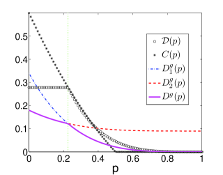
Figure 1: (Color online) Discord $D(p)$, concurrence $C(p)$ and the geometry measure of discord $D^{g}(p)$ under PDC, as functions of $p$, for the input state taken as $c_{1}=1$, $c_{2}=-c_{3}$ and $c_{3}=0.6$.

In Fig. 1, we show that the GMQD is monotonically non-decreasing with respect to the quantum discord. When $p\leq 1-\sqrt{3/5}$, the GMQD decreases while the quantum discord keeps constant. It is remarkable that regime where the quantum discord is unaffected by the noisy environment is important for the implementation of a quantum computer Mazzola2010 . The entanglement may disappear completely after a finite time, known as entanglement-sudden-death (ESD) Yu2004 ; Eberly2007 ; Yu2009 . In cases where ESD occurs, contrarily, the quantum discord is more robust than the concurrence Werlang2009 , so does the GMQD, see Fig. 1. The discontinuity of the decay rates occurs at $p=1-\sqrt{3/5}$ (see the dotted line in Fig. 1). For the GMQD, this kind of sudden change occurs when the maximum singular value of the matrix $\mathcal{R}^{\prime}$ jumps from one family to another one, see $D_{1}^{g}(p)$ and $D_{2}^{g}(p)$ in Fig. 1.

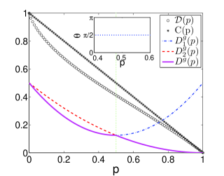
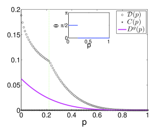
Figure 2: (Color online) Discord $D(p)$, concurrence $C(p)$ and the geometry measure of discord $D^{g}(p)$ as functions of $p$. The left subfigure is plotted for the case of the Bell state ($c_{1}=c_{2}=c_{3}=-1$) under the ADC. The right subfigure is plotted for the case of the states (33) with $c_{1}=0.5$, $c_{2}=0$, $c_{3}=0.5$ and $d=-0.5$ under the PDC. In the inset of each figure, we plot the values of $\theta$ which maximize $\mathcal{I}(\rho(p)|\{E_{k}(\theta,\phi)\})$ at different $p$, where $E_{k}(\theta,\phi)=(\openone+\vec{n}\cdot\vec{\sigma})/2$ with $n=(\sin\theta\cos\phi,\sin\theta\sin\phi,\cos\theta)^{T}$.

However, the sudden change in decay rates of the GMQD may not imply that of the quantum discord, and vice versa. For instance of the former, we consider the second example, a Bell state ($c_{1}=c_{2}=c_{3}=-1$) under the ADC. Substituting $c_{i}=-1$ ($i=1,2,3$) into Eq. (27), we obtain

$$D_{\mathrm{ADC}}^{g}(p) = \min\left\{D_{1}^{g}(p),D_{2}^{g}(p)\right\},$$

$$D_{1}^{g}(p)=\frac{1}{2}(1-3p+3p^{2}), D_{2}^{g}(p)=\frac{1}{2}(1-p)^{2}.$$ (32)

From the left subfigure of Fig. 2, we can see that the sudden change in the decay rates of the GMQD occurs at $p=0.5$, where the quantum discord obtained numerically does not display any discontinuity in the first derivative. To demonstrate that the sudden change is decay rates of the quantum discord may not imply the GMQD, we consider the third example—the input state

$$\rho=\frac{1}{4}\left(\openone\otimes\openone+\sum_{i=1}^{3}c_{i}\sigma_{i}\otimes\sigma_{i}+d\sigma_{3}\otimes\openone+d\openone\otimes\sigma_{3}\right)$$ (33)

under the PDC. Here the parameters are choose as $c_{1}=0.5$, $c_{2}=0$, $c_{3}=0.5$ and $d=-0.5$. After some algebras similar to the case where the input states are Bell diagonal states, the GMQD is obtained as $D^{g}_{\mathrm{PDC}}=(1-p)^{4}/16$. From the right subfigure of Fig. 2, we can see that the sudden change in decay rates of the quantum discord occurs at $p\simeq 0.22$, where the GMQD does not display any discontinuity in the first derivative.

In the following, we give a general analysis on the sudden change in decay rates of the GMQD and the quantum discord. Hereafter, we assume that the elements of the two-qubit density matrix are smooth functions of $p$, then the sudden changes in decay rate of both the GMQD and the quantum discord are induced by the optimization procedure involved in their definitions. For the GMQD, the optimization procedure is to find the closest one $\tilde{\chi}$ among the zero-discord state $\chi=p_{1}\Pi_{1}\otimes\rho_{1}+p_{2}\Pi_{2}\otimes\rho_{2}$. Here $\Pi_{1}$ and $\Pi_{2}$ are orthogonal projective operators and can be expressed by $\Pi_{1}=(\openone+\sum_{i=1}^{3}e_{i}\sigma_{i})/2$ and $\Pi_{2}=\openone-\Pi_{1}$ with $e_{i}$ the components of a unit vector $e=(e_{1},e_{2},e_{3})^{T}$ on the Bloch sphere. In Ref. Dakic2010 , Dakić et al. obtain the results (7) where $k_{\mathrm{max}}$ can be expressed by

$$k_{\mathrm{max}}(p)=\max_{|e|=1}[e^{T}K(p)e].$$ (34)

So the sharp features of the GMQD are caused by the optimization over $e$. Then the closest zero-discord state is given by $\tilde{\chi}=\tilde{p}_{1}\tilde{\Pi}_{1}\otimes\tilde{\rho}_{1}+\tilde{p}_{2}\tilde{\Pi}_{2}\otimes\tilde{\rho}_{2}$ where $\tilde{\Pi}_{1}(p)=(\openone+\sum_{i=1}^{3}\tilde{e}_{i}(p)\sigma_{i})/2$ with $\tilde{e}(p)$ the eigenvector of $K(p)$ with the largest eigenvalue. We do not care about the other parameters in the $\tilde{\chi}$ since they have nothing to do with the GMQD. Hence, the sudden change in decay rates of the GMQD corresponds to the sudden change of $\tilde{e}(p)$. On the other hand, for the quantum discord, the optimization procedure is to find an optimal projective measurement $\{\tilde{E}_{k}\}$ to access the classical correlation over the set of projective measurement $\{E_{k}\}$. Then the sudden change in the decay rates of the quantum discord is induced by the sudden change of $\{\tilde{E}_{k}(p)\}$ with respect to $p$. In a similar way to $\tilde{\Pi}_{i}$, the optimal projective operator can be represented by $\tilde{E}_{1}(p)=(\openone+\sum_{i=1}^{3}\tilde{n}_{i}\sigma_{i})/2$ and $\tilde{E}_{2}=\openone-\tilde{E}_{1}$ with $n_{i}$ the components of a unit vector $\tilde{n}=(\tilde{n}_{1},\tilde{n}_{2},\tilde{n}_{3})^{T}$ on the Bloch sphere, or equivalently $\tilde{n}=(\sin\theta\cos\phi,\sin\theta\sin\phi,\cos\theta)^{T}$. In the inset of Fig. 2, we plot $\theta$ for the optimized measurement $\tilde{E}_{1}(\theta,\phi)$ for different point $p$. For the second example (a Bell state under the ADC), the output state are invariant under a rotation $R_{z}(\varphi)=\exp(i\varphi\sigma_{z}^{A}/2)\otimes\exp(i\varphi\sigma_{z}^{B}/2)$ and $\mathcal{I}(\rho|\{E_{k}\})$ are invariant under local unitary transformation, so if $\{\tilde{E}_{k}(\theta,\phi)\}$ is the optimal measurement, then $\{\exp(i\varphi\sigma_{z}^{A}/2)E_{k}(\theta,\phi)\exp(-i\varphi\sigma_{z}^{A}/2)\}=\{E(\theta,\phi-\varphi)\}$ is also the optimal measurement. In other words, the optimization procedure is only relevant to $\theta$. In the inset of the left part of Fig. 2, we can see that there is no sudden change of $\theta$. For the third example, in the inset of the right part of Fig. 2, we can see that a sudden change of $\theta$ occurs at $p\simeq 0.22$, where the decay rate of the quantum discord is discontinuous. And we do not care about $\phi$ because the sudden change of the optimal measurement has already been reflected through the discontinuity of $\theta$.

Notice that the optimal $\tilde{E}_{k}(p)$ and $\tilde{\Pi}_{k}(p)$ are both projective operators. For general states, $\{\tilde{E}_{k}(p)\}$ is not the same as $\{\tilde{\Pi}_{k}(p)\}$, which is reflected in the disagreement of their individual sudden change in decay rate. However, at least for the Bell diagonal states, $\{\tilde{E}_{k}(p)\}$ is the same as $\{\tilde{\Pi}_{k}(p)\}$, or equivalently $\tilde{n}(p)=\tilde{e}(p)$. This can be seen from the following analysis. In Ref. Luo2008 , Luo solved the optimization analytically for the Bell diagonal states, and $\tilde{n}$ is found to be the eigenvector of $RR^{T}$ with the largest eigenvalue. On the other hand, in Ref. Dakic2010 , Dakić et al. showed that $\tilde{e}$ is the eigenvector of $K=xx^{T}+RR^{T}$ with the largest eigenvalue. For the Bell states $K=RR^{T}$ due to $x=0$. Hence, we get $\tilde{n}(p)=\tilde{e}(p)$. So it is concluded the sudden change in decay rates of the GMQD that of the quantum discord occurs simultaneously if the states are the Bell diagonal states.

IV Conclusion and discussion

In conclusion, we have considered the dynamics of the GMQD under decoherence. We showed that the GMQD of a two-qubit state can be obtained through the singular values of a special $3\times 4$ matrix whose elements are the expectation values of the Pauli matrices of the two qubits. With the help of the Heisenberg picture, we got the analytic results of the geometric measure of the quantum discord for states under three typical kinds of quantum decoherence channels. We showed that the sudden change in decay rates of the GMQD does not always imply that of the quantum discord, and vice versa. And at least for the Bell diagonal states, their individual sudden changes in decay rate are accordance.

In the present work, we adopt the Hilbert-Schmidt norm as the distance between two states. Besides, there exist other quantities for measuring the distance, e.g. the relative entropy Modi2010 and the Bures distance. For the Hilbert-Schmidt distance, we show the disagreement between the GMQD and the quantum discord on reflecting the sudden changes in decay rates, so what about other kinds of the distance? Is this disagreement a property of the general geometric measure of quantum discord, or just of the geometry measure based on the Hilbert-Schmidt distance? Most recently, the phenomena of the sudden change in decay rates have been tested experimentally JSXu2010 .

V Acknowledgment

The authors thank B. Dakić and M. Ali for helpful communications, and the referees for the suggestion making the present work improved. X. Wang is supported by NSFC with grant No. 10874151, 10935010, NFRPC with grant No. 2006CB921205; and the Fundamental Research Funds for the Central Universities. Z. Xi is supported by the Superior Dissertation Foundation of Shaanxi Normal University (S2009YB03). Z. Sun is supported by the National Nature Science Foundation of China with Grants No. 10947145; Science Foundation of Zhejiang Province with Grant No. Y6090058.

References

- (1) H. Ollivier and W. H. Zurek, Phys. Rev. Lett. 88, 017901 (2001).
- (2) L. Henderson and V. Vedral, J. Phys. A 34, 6899 (2001).
- (3) A. Datta, A. Shaji, and C. M. Caves, Phys. Rev. Lett. 100, 050502 (2008).
- (4) B. P. Lanyon, M. Barbieri, M. P. Almeida, and A. G. White, Phys. Rev. Lett. 101, 200501 (2008).
- (5) S. Luo, Phys. Rev. A77, 042303 (2008).
- (6) R. Dillenschneider, Phys. Rev. B78, 224413 (2008).
- (7) M. S. Sarandy, Phys. Rev. A80, 022108 (2009).
- (8) M. Ali, A. R. P. Rau, and G. Alber, Phys. Rev. A, 81, 042105 (2010).
- (9) G. Adesso and A. Datta, Phys. Rev. Lett. , 105, 030501 (2010).
- (10) P. Giorda and M. G. A. Paris, Phys. Rev. Lett. , 105, 020503 (2010).
- (11) Y.-X Chen and S.-W Li, Phys. Rev. A81, 032120 (2010).
- (12) L. Mazzola, J. Piilo, S. Maniscalco, arXiv:1001.5441v2.
- (13) J. Maziero, T. Werlang , F. F. Fanchini, L. C. Céleri, and R. M. Serra, Phys. Rev. A81, 022116 (2010).
- (14) J. Maziero, L. C. Céleri, R. M. Serra, and V. Vedral, Phys. Rev. A80, 044102 (2009).
- (15) T. Werlang, S. Souza, F. F. Fanchini, and C. J. Villas Boas, Phys. Rev. A80, 024103 (2009).
- (16) B. Wang, Z.-Y Xu, Z.-Q. Chen, and M. Feng, Phys. Rev. A81, 014101 (2010).
- (17) F. F. Fanchini, T. Werlang, C. A. Brasil, L. G. E. Arruda, and A. O. Caldeira, Phys. Rev. A81, 052107 (2010).
- (18) J.-S. Xu, X.-Y. Xu, C.-F. Li, C.-J. Zhang, X.-B. Zou, and G.-C Guo, Nat. Commun. 1, 7 (2010).
- (19) B. Dakić, V. Vedral, and Č. Brukner, arXiv:1004.0190v1.
- (20) K. Modi, T. Paterek, W. Son, V. Vedral, and M. Williamson, Phys. Rev. Lett. 104, 080501 (2010).
- (21) Y.-X. Chen and Z. Yin, arXiv:1002.0176v1 (2010).
- (22) A. Ferraro, L. Aolita, D. Cavalcanti, F. M. Cucchietti, and A. Acin, arXiv:0908.3157v3.
- (23) T. Werlang and G. Rigolin, Phys. Rev. A81, 044101 (2010).
- (24) J. Maziero, L. C. Céleri, and R. M. Serra, arXiv:1004.2082v1.
- (25) B. Bylicka and D. Chruściński, arXiv:1004.0434v1.
- (26) A. Datta, eprint arXiv:1003.5256v1.
- (27) A. Datta and S. Gharibian, Phys. Rev. A79, 042325 (2009).
- (28) V. Vedral, M. Plenio, M. Rippin, and P. Knight, Phys. Rev. Lett. 78, 2275 (1997).
- (29) T.-C. Wei and P. M. Goldbart, Phys. Rev. A68, 042307 (2003).
- (30) T. Yu and J. H. Eberly, Phys. Rev. Lett. 93, 140404 (2004).
- (31) J. H. Eberly and T. Yu, Science 316, 555 (2007).
- (32) T. Yu and J. H. Eberly, Science 323, 598 (2009).
- (33) T. Yu and J.H. Eberly, J. Mod. Opt. 54, 2289 (2007).
- (34) D. Zhou and R. Joynt, arXiv:1006.5474.
- (35) D. Zhou, G.-W. Chern, J. Fei, and R. Joynt, arXiv:1007.1749.
- (36) M. Koashi and A. Winter, Phys. Rev. A 69, 022309 (2004).
- (37) L.-X. Cen, X.-Q. Li, J.S. Shao, and Y.J. Yan, arXiv:1006.4727.
- (38) B. Groisman, S. Popescu, and A. Winter, Phys. Rev. A72, 032317 (2005).
- (39) J. Schlienz and G. Mahler, Phys. Rev. A52, 4396 (1995).
- (40) X. Wang, A. Miranowicz, Y.-X Liu, C. P. Sun, and F. Nori, Phys. Rev. A81, 022106 (2010).
- (41) M. A. Nielsen, I. L. Chuang, Quantum Computation and Quantum Information, (Cambridge University Press, Cambridge, UK, 2000).
- (42) J. Preskill, Lecture Notes for Physics 219: Quantum Information and Computation (Caltech, Pasadena, CA, 1999), Chap. 3, http://www.theory.caltech.edu/people/preskill/ph229/.
- (43) R. Horodecki and M. Horodecki, Phys. Rev. A54, 1838 (1996).
- (44) S. Hill and W. K. Wootters, Phys. Rev. Lett. 78, 5022 (1997).
- (45) W. K. Wootters, Phys. Rev. Lett. 80, 2245 (1998).