Abstract

We estimate the QCD effective charge $\alpha_{s}$ in the low-energy region by exploiting the conventional meson spectrum within a relativistic quantum-field model based on analytic confinement. The ladder Bethe-Salpeter equation is solved for the masses of two-quark bound states. We found a new, independent and specific infrared-finite behavior of QCD coupling below energy scale 1 GeV. Particularly, an infrared-fixed point is extracted at $\alpha_{s}(0)\simeq 0.757$ for confinement scale $\Lambda=345$ MeV. As an application, we estimate masses of some intermediate and heavy mesons and obtain results in reasonable agreement with recent experimental data.

PACS: 11.10.St, 12.38.Aw, 12.38.Qk, 12.39.-x, 12.40.Yx, 14.40.-n

1 Introduction

The study of QCD behavior at large distances is an active field of research in particle physics because many interesting and novel behaviors are expected at low energies below 1 GeV (see, e.g., [1, 2]). Understanding of a number of phenomena such as quark confinement, hadronization, the effective coupling and nonvanishing vacuum expectation values, etc. requires a correct description of hadron dynamics in the infrared (IR) region. However, the well-established conventional perturbation theory cannot be used effectively in the IR region and it is required either to supply some additional phenomenological parameters (e.g., ”effective masses”, anomalous vacuum averages, etc.), or to use some nonperturbative methods (lattice simulations [3], power correction [4], string fragmentation [5], Dyson-Schwinger equations, etc.). There exists a phenomenological indication in favor of a smooth transition from short distance to long-distance physics [4].

One of the fundamental parameters of nature, the QCD effective coupling $\alpha_{s}$ can provide a continuous interpolation between the asymptotical free state, where perturbation theory works well, and the hadronization regime, where nonperturbative techniques must be employed.

QCD predicts the functional form of the energy dependence of $\alpha_{s}$ on energy scale $Q$, but its actual value at a given $Q$ must be obtained from experiment. This dependence is described theoretically by the renormalization group equations and measured at relatively high energies [6, 7]. A self-consistent and physically meaningful prediction of the QCD effective charge in the IR regime remains one of the actual problems in particle physics.

The present paper is aimed to determine the QCD effective charge in the low-energy region by exploiting the hadron spectrum. In doing so we extend our previous investigations [8, 9, 10], where we provided new, independent, analytic and numerical estimates on the lowest glueball mass, conventional meson spectrum and the weak decay constants by using a fixed (”frozen”) value of $\alpha_{s}$. The obtained results were in reasonable agreement with experimental evidence.

Below we take into account the dependence of $\alpha_{s}$ on mass scale $M$ and develop a phenomenological model to describe the IR behavior of $\alpha_{s}$. We determine the meson masses by solving the ladder Bethe-Salpeter (BS) equations for two-quark bound states. The consideration is based on a relativistic quantum-field model with analytic confinement (AC) and has a minimal number of parameters, namely, the confinement scale $\Lambda$ and the constituent quark masses $m_{f},~{}(f=\{ud,s,c,b\})$. First, we derive the meson mass formula and adjust the model parameters by fitting heavy meson masses ($M\geq 2$ GeV). Hereby, we determine corresponding values of $\alpha_{s}(M)$ from a smooth interpolation of the newest experimental data on the QCD coupling constant. Having adjusted model parameters, we estimate $\alpha_{s}(M)$ in the low-energy domain by exploiting meson masses below $\sim 1$ GeV. As an application, we estimate some intermediate and heavy meson masses ($1<M<9.5$ GeV). Finally, we extract a specific IR-finite behavior of the QCD coupling and conclude briefly recalling the comparison with often quoted results and recent experimental data.

2 Effective Coupling of QCD

The polarization of QCD vacuum causes two opposite effects: the color charge $g$ is screened by the virtual quark-antiquark pairs and antiscreened by the polarization of virtual gluons. The competition of these effects results in a variation of the physical coupling under changes of distance $\sim 1/Q$, so QCD predicts a dependence $\alpha_{s}\doteq g^{2}/(4\pi)=\alpha_{s}(Q)$. This dependence is described theoretically by the renormalization group equations and determined experimentally at relatively high energies [6, 7].

Figure 1: Measurements of $\alpha_{s}$ as a function of the respective energy scale $Q$ versa QCD predictions (curves) [11].

Nowadays, determinations of $\alpha_{s}$ remain at the forefront of experimental studies and tests of QCD. Recent developments on this subject were summarized in a number of articles [2, 11, 12]. Summary of the recent experimental measurements of $\alpha_{s}$ (Fig. 1) and particular values of $\alpha_{s}$ at intermediate energies (Tab. 1) are given by referring to [7, 11].

Note that there are two separate $q^{2}$ scale regions in which a running coupling may be considered. The spacelike region ($q^{2}=-Q^{2}<0$ with relativistic momentum transfer $Q^{2}$) is related to scattering processes while timelike domain ($q^{2}=M^{2}>0$, where $M$ is the hadron mass) is often used for annihilation and decay processes. The consistent description of QCD effective coupling $\alpha_{s}$ in these domains remains the goal of many studies because only asymptotically the two definitions can be identified but at low momentum they can be very different (see, e.g. [13]).

Particularly, the behavior of one-loop analytic running coupling [14] in timelike and spacelike domains is plotted in Fig. 2.

Many quantities in hadron physics are affected by the IR behavior of the coupling in different amounts. Nevertheless, the long-distance behavior of $\alpha_{s}$ is not well defined, it needs to be more specified [15, 16, 17] and correct description of QCD effective coupling in the IR regime remains one of the actual problems in particle physics. Particularly, one of the most precise determinations of $\alpha_{s}$ near the low-energy region is done by studying $\tau$-lepton decays reporting central values ranging from 0.318 to 0.344 [18, 19, 20].

Figure 2: The one-loop massless analytic running coupling in the spacelike and timelike domains (taken from [14]).

An attempt to extrapolate the perturbative approach to the long-distance QCD has been made, it has been suggested that $\alpha_{s}$ freezes at a finite and moderate value [24], and this behavior could be the reason for the soft transition between short and long distance behaviors.

Process	$Q{\mbox{\rm~{}[GeV]}}$	$\alpha_{s}(Q)$	Ref:
$\tau$-decays	1.78	0.330 $\pm$ 0.014	[11]
$Q\bar{Q}$ states	4.1	0.239 $\pm$ 0.012	[21]
$\Upsilon$ decays	4.75	0.217 $\pm$ 0.021	[22]
$Q\bar{Q}$ states	7.5	0.1923 $\pm$ 0.0024	[11]
$\Upsilon$ decays	9.46	0.184 $\pm$ 0.015	[11]
$e^{+}e^{-}$ jets	14.0	0.170 $\pm$ 0.021	[23]

Table 1: Some measurements of $\alpha_{s}$ at intermediate energies.

Different nonperturbative approaches have been proposed to deal with the IR properties of $\alpha_{s}$. Particularly, methods, based on gauge-invariant SDE, concluded that an IR-finite coupling constant may be obtained from first principles [25]. New solutions for the gluon and ghost SDE have been obtained with better approximations which led to a new value for the IR coupling constant at the origin [26, 27]. Many works within the lattice simulations have been devoted in recent years to the study of the QCD running coupling constant either in the perturbative regime [28, 29] or in the deep IR domain [30]. Note that the results of various nonperturbative methods for the QCD invariant coupling may differ among themselves in the IR region due to the specifications of the used methods and approximations. Particularly, the results obtained by lattice simulations and SDE methods demonstrate a considerable variety of IR behaviors of $\alpha_{s}$.

An extraction of experimental data of $\alpha_{s}^{exp}(Q^{2})$ below 1 GeV compared with the meson spectrum within analytic perturbation theory has been performed [31] and a summary of data was presented (see Fig. 2). The earliest attempts to obtain $\alpha_{s}$ in the IR region were made in the framework of the quark-antiquark potential models by using the Wilson loop method [32, 33, 34, 35, 36]. Convenient interpolation formulas between the large momentum perturbative expression and a finite IR-fixed point have been used in hadron spectrum studies with ${\alpha_{s}^{0}/\pi}\simeq 0.19-0.25$ [36]. Within a fully relativistic treatment it was shown that a $\rho$-meson mass much heavier than the $\pi$ mass could be obtained with ${\alpha_{s}^{0}/\pi}\simeq 0.265$ [37] while a similar result within a one-loop analytic coupling method predicted ${\alpha_{s}^{0}/\pi}\simeq 0.44$ [38]. A phenomenological hypothesis was adopted that the gluon acquires an effective dynamical mass $m_{g}\approx 370MeV$ (at $\Lambda_{QCD}\approx 300MeV$) that resulted in ${\alpha_{s}^{0}/\pi}\simeq 0.26$ [39]. Various event shape in $e^{+}e^{-}$ annihilation can be reproduced with an averaged value $\left\langle{\alpha_{s}^{0}/\pi}\right\rangle\simeq 0.2$ on interval $\leq 1~{}GeV$ [4].

3 Model

Color confinement in QCD is an attempt to explain the physics phenomenon that color charged particles are not observed. However, the reasons for quark confinement may be somewhat complicated. Particularly, within a quantum-field model, the quark confinement may be explained as the absence of quark poles and thresholds in Green’s function. Following this idea, the conception of AC assumes that the QCD vacuum is realized by the self-dual vacuum gluon fields which are stable versus local quantum fluctuations and related to the confinement and chiral symmetry breaking [40]. This vacuum gluon field serves as the true minimum of the QCD effective potential [41]. The vacuum of the quark-gluon system has the minimum at the nonzero self-dual homogenous background field with constant strength. Then, the quark and gluon propagators in the background gluon field represent entire analytic functions in Euclidean space [42]. In previous papers [43, 10]] we developed relativistic quantum-field models with AC. Similar ideas have been realized in infrared confinement by introducing an IR cutoff within a Nambu-Jona-Lasino model [44, 45].

The Bethe-Salpeter equation is an important tool for studying the relativistic two-particle bound states in a field theory framework [46]. Numerical calculations indicate that the ladder BS equation with a phenomenological model can give satisfactory results (for a review, see [47]). Particularly, a BS formalism adjusted for QCD was developed to extract values of $\alpha_{s}$ below 1 GeV by comparison with known meson masses [31].

Our purpose is to investigate QCD effective (running) charge in the low-energy levels by exploiting the spectrum of conventional mesons. For the spectra of two-quark bound states we consider a relativistic quantum-field model based on analytic (or infrared) confinement and solve the ladder BS equation.

Following previous papers [43, 10] we consider a model Lagrangian:

$${\cal L}=-{1\over 4}\left(F^{A}_{\mu\nu}-gf^{ABC}{\cal A}^{B}_{\mu}{\cal A}^{C}_{\nu}\right)^{2}+\sum_{f}\left(\bar{q}^{a}_{f}\left[\gamma_{\alpha}\partial^{\alpha}-m_{f}+g\Gamma^{\alpha}_{C}{\cal A}^{C}_{\alpha}\right]^{ab}q^{b}_{f}\right)\,,$$ (1)

where ${\cal A}^{C}_{\alpha}$ is the gluon adjoint representation ($\alpha=\{1,...,4\}$); $F^{A}_{\mu\nu}=\partial^{\mu}{\cal A}_{\nu}^{A}-\partial^{\nu}{\cal A}_{\mu}^{A}$; $f^{ABC}$ is the $SU_{c}(3)$ group structure constant ($\{A,B,C\}=\{1,...,8\})$; $q_{f}^{a}$ is the quark spinor of flavor $f$ with color $a=\{1,2,3\}$ and mass $m_{f}$; $g$ is the coupling strength, $\Gamma^{\alpha}_{C}=i\gamma_{\alpha}t^{C}$; and $t^{C}$ is the Gell-Mann matrices.

Remember, that within the model the quark and gluon propagators $\tilde{S}(\hat{p})$ and $\tilde{D}(p)$ in (1) are entire analytic functions in the Euclidean space.

3.1 Confinement and Green’s Functions

The effective charge is strongly governed by the detailed dynamics of the strong interaction and may depend on some of the most fundamental Green s functions of QCD, such as the gluon and quark propagators [48]. The Green’s functions in QCD are tightly connected to confinement and are ingredients for hadron phenomenology. However, any widely accepted and rigorous analytic solutions to these propagators are still missing. One may encounter difficulties by defining the explicit quark and gluon propagator at the confinement scale. Nowadays, IR behaviors of the quark and gluon propagators are not well-established and need to be more specified [15].

The matrix elements of hadron processes at large distance are integrated characteristics of the vertices, quark and gluon propagators and the solution of the BS equation should not be too sensitive on the details of propagators. Taking into account the correct global symmetry properties and their breaking (also by introducing additional physical parameters) may be more important than the working out in detail of propagators (e.g., [49]). In previous papers we exploited simple forms of quark and gluon propagators [10, 43] which were entirely analytic functions in Euclidean space and behaved similarly to the explicit propagators dictated by AC [42].

Following [10] we introduce the quark propagator as follows:

$$\tilde{S}_{m}^{ab}(\hat{p})=~{}\delta^{ab}{i\hat{p}+m_{f}[1\pm\gamma_{5}~{}\omega(m_{f}/\Lambda)]\over\Lambda m_{f}}\exp\left\{-{p^{2}+m_{f}^{2}\over 2\Lambda^{2}}\right\}\,,$$ (2)

where $\hat{p}=p_{\mu}\gamma_{\mu}$ and $\omega(z)=(1+z^{2}/4)^{-1}$. The sign ”$\pm$” corresponds to the self- and antiself-dual modes of the background gluon fields. In (2) chiral symmetry breaking is induced by AC. The interaction of the quark spin with the background gluon field results in a singular behavior $\tilde{S}_{\pm}(\hat{p})\sim 1/m_{f}$ in the massless limit $m_{f}\to 0$. This expresses the zero-mode solution (the lowest Landau level) of the massless Dirac equation in the presence of an external gluon background field and generates a nontrivial quark condensate [10] indicating the broken chiral symmetry as $m_{f}\to 0$.

Recent theoretical results predict an IR behavior of the gluon propagator. A gluon propagator identical to zero at the momentum origin was considered in [50, 51] while another propagator was of order $1/m_{g}^{2}$ [4], where $m_{g}$ is the dynamical gluon mass [52]. A renormalization group analysis [53] and numerical lattice studies simulating the gluon propagator are consistent with an IR-finite behavior [54]. We consider a gluon propagator

$$\tilde{D}_{\mu\nu}^{AB}(p)=\delta^{AB}\delta_{\mu\nu}{1-\exp\left(-{p^{2}/\Lambda^{2}}\right)\over p^{2}}=\delta^{AB}\delta_{\mu\nu}\int\limits_{0}^{1/\Lambda^{2}}\!\!\!ds\,e^{-sp^{2}}\,.$$ (3)

It represents a modification of gluon propagator defined in [10] and exhibits an explicit IR-finite behavior $\tilde{D}(0)\sim 1/\Lambda^{2}$. For simplicity $\tilde{D}(p)$ in (3) is given in Feynman gauge.

Note that the propagators in Eqs. (2) and (3) do not have any singularities in the finite $p^{2}$ plane in Euclidean space, thus indicating the absence of a single quark (gluon) in the asymptotic space of states. In fact, an IR parametrization is hidden in the confinement scale $\Lambda$.

3.2 Two-quark Bound States

We allow that the coupling remains weak ($\alpha_{s}<1$) in the hadronization region. Then, the consideration may be restricted within the ladder approximation sufficient to estimate the meson spectrum with reasonable accuracy. The leading-order contribution to the two-quark ($q\bar{q}$) bound states is determined by the partition function

$$Z_{q\bar{q}}=\int\!\!\!\int\!\!{\mathcal{D}}\bar{q}{\mathcal{D}}q\exp\left\{-(\bar{q}S^{-1}q)+{g^{2}\over 2}\left\langle(\bar{q}\Gamma{\cal A}q)(\bar{q}\Gamma{\cal A}q)\right\rangle_{D}\right\}\,,$$

$$\langle(\bullet)\rangle_{D}\doteq\int\!\!{\mathcal{D}}{\cal A}~{}e^{-{1\over 2}({\cal A}D^{-1}{\cal A})}(\bullet)\,.$$ (4)

Our model has a minimal number of parameters, namely, the scale of confinement $\Lambda$ and the constituent quark masses ($m_{ud},m_{s},m_{c},m_{b}$).

Below we briefly introduce the basic steps entering into our model on the example of the quark-antiquark bound states [10] defined by $Z_{q\bar{q}}$ in (4).

First, we allocate the one-gluon exchange between colored biquark currents

$${\cal L}_{2}={g^{2}\over 2}\sum\limits_{f_{1}f_{2}}\int\!\!\!\int dx_{1}dx_{2}\left(\bar{q}_{f_{1}}(x_{1})i\gamma_{\mu}t^{A}q_{f_{1}}(x_{1})\right)D_{\mu\nu}^{AB}(x_{1},x_{2})\left(\bar{q}_{f_{2}}(x_{2})i\gamma_{\nu}t^{B}q_{f_{2}}(x_{2})\right).$$ (5)

and isolate the color-singlet combinations. We perform a Fierz transformation

$$(i\gamma_{\mu})\delta^{\mu\nu}(i\gamma_{\nu})=\sum_{J}C_{J}\cdot O_{J}~{}O_{J}\,,\qquad J=\{S,P,V,A,T\}\,,$$

where $C_{J}=\{1,1,1/2,-1/2,0\}$ and $O_{J}=\{I,i\gamma_{5},i\gamma_{\mu},\gamma_{5}\gamma_{\mu},i[\gamma_{\mu},\gamma_{\nu}]/2\}$. For systems consisting of quarks with different masses it is important to go to the relative co-ordinates in the center-of-masses system and introduce the relative masses $\xi_{i}\doteq m_{i}/(m_{1}+m_{2})$. Then, introduce a system of orthonormalized basis functions $\{U_{Q}(x)\}$, where $Q=\{n_{r},{\em l},\mu\}$ are the radial, orbital and magnetic quantum numbers. Diagonalize ${\cal L}_{2}$ on basis $\{U_{Q}(x)\}$ and use a Gaussian path-integral representation for the exponential

$$e^{{\cal L}_{2}}\doteq e^{{g^{2}\over 2}\sum\limits_{{\cal N}}({\cal J}_{{\cal N}}^{2})}=\left\langle e^{g(B_{{\cal N}}{\cal J}_{{\cal N}})}\right\rangle_{B}\,,\qquad\left\langle(\bullet)\right\rangle_{B}\doteq\int\prod\limits_{N}{\mathcal{D}}B_{N}~{}e^{-{1\over 2}(B_{{\cal N}}^{2})}(\bullet)\,,\qquad\left\langle 1\right\rangle_{B}=1$$

by introducing a colorless biquark current ${\cal J}_{{\cal N}}$ and auxiliary meson fields $B_{\cal N}$ with ${\cal N}=\{Q,J,f_{1},f_{2}\}$. Then

$$Z_{q\bar{q}}=\left\langle\int\!\!\!\int\!\!{\mathcal{D}}\bar{q}{\mathcal{D}}q\exp\left\{-(\bar{q}S^{-1}q)+g(B_{{\cal N}}{\cal J}_{{\cal N}})\right\}\right\rangle_{B}\,.$$

By taking explicit path integration over quark variables we obtain

$$Z_{q\bar{q}}\rightarrow Z=\left\langle\exp\left\{{\rm Tr}\ln\left[1+g(B_{{\cal N}}V_{{\cal N}})S\right]\right\}\right\rangle_{B}\,,$$

where $V_{\cal N}(x,y)$ is a vertex function.

Introduce a hadronization ansatz and this will identify $B_{\cal N}(x)$ with meson fields carrying quantum numbers ${\cal N}$. We isolate all quadratic field configurations ($\sim B^{2}_{\cal N})$ in the ”kinetic” term and rewrite the partition function for mesons [10]:

$$Z=\int{\prod\limits_{\cal N}{\mathcal{D}}B_{\cal N}\,\exp\left\{{-\frac{1}{2}\sum\limits_{{\cal NN^{\prime}}}(B_{\cal N}\,[\delta^{{\cal NN^{\prime}}}+\alpha_{s}\lambda_{\cal NN^{\prime}}]\,B_{{\cal N^{\prime}}})-W_{res}[B_{\cal N}]}\right\}}\,,$$ (6)

where the interaction between mesons is described by the residual part $W_{res}[B_{\cal N}]\sim 0(B_{\cal N}^{3})$.

The leading-order term of the polarization operator is

$$\alpha_{s}\lambda_{{\cal NN^{\prime}}}(z)\doteq\int\!\!\!\int\!\!dxdy\,U_{\cal N}(x)\,\alpha_{s}\lambda_{JJ^{\prime}}(z,x,y)\,U_{{\cal N^{\prime}}}(y)\,,$$ (7)

and the Fourier transform of its kernel reads

$$\alpha_{s}\lambda_{{JJ^{\prime}}}(p,x,y)\doteq\alpha_{s}\int\!\!dz\,e^{ipz}\lambda_{JJ^{\prime}}(z,x,y)$$

$$={4g^{2}\sqrt{C_{J}\,C_{J^{\prime}}}\over 9}\sqrt{D(x)D(y)}\int\!\!{d^{4}k\over(2\pi)^{4}}~{}e^{-ik(x-y)}{\rm Tr}\left[O_{J}\tilde{S}_{m_{1}}\left(\hat{k}+\xi_{1}\hat{p}\right)O_{J^{\prime}}\tilde{S}_{m_{2}}\left(\hat{k}-\xi_{2}\hat{p}\right)\right]\,,$$ (8)

where ${\rm Tr}\doteq{\rm Tr}_{c}{\rm Tr}_{\gamma}\sum_{\pm}$; ${\rm Tr}_{c}$ and ${\rm Tr}_{\gamma}$ are traces taken on color and spinor indices, correspondingly, while $\sum_{\pm}$ implies the sum over self-dual and antiself-dual modes.

We diagonalize the polarization kernel on the orthonormal basis $\{U_{\cal N}\}$:

$$\int\!\!\!\int\!\!dxdy\,U_{{\cal N}}(x)\lambda_{{JJ^{\prime}}}(p,x,y)U_{{\cal N}^{\prime}}(y)=\delta^{{\cal NN}^{\prime}}~{}\lambda_{{\cal N}}(-p^{2})$$

that is equivalent to the solution of the corresponding ladder BS equation. We rewrite

$$\lambda_{{\cal N}}(-p^{2}) = {8\,C_{J}\over 3\pi^{3}}\int\!\!{d^{4}k}\left|V_{J}(k)\right|^{2}\Pi_{\cal N}(k,p)\,,$$ (9)

$$V_{J}(k) \doteq \int\!\!d^{4}x\,U_{J}(x)\sqrt{D(x)}\,e^{-ikx}\,,$$

$$\Pi_{\cal N}(k,p) \doteq {1\over 24}{\rm Tr}\left[O_{J}\tilde{S}_{m_{1}}\left(\hat{k}+\xi_{1}\hat{p}\right)O_{J^{\prime}}\tilde{S}_{m_{2}}\left(\hat{k}-\xi_{2}\hat{p}\right)\right]\,,$$

where $V_{J}(k)$ is a vertex and $\Pi_{\cal N}(k,p)$ is the kernel of the polarization operator.

In relativistic quantum-field theory a stable bound state of $n$ massive particles shows up as a pole in the S-matrix with a center of mass energy. Accordingly, the physical mass of the meson may be derived from the equation

$$1+\alpha_{s}\lambda_{{\cal N}}(M_{{\cal N}}^{2})=0\,,\qquad-p^{2}=M_{\cal N}^{2}\,.$$ (10)

Then, with a renormalization

$$(B_{\cal N}[1+\alpha_{s}\lambda_{\cal N}(-p^{2})]B_{\cal N})=(B_{\cal N}[1+\alpha_{s}\lambda_{{\cal N}}(M_{{\cal N}}^{2})+\alpha_{s}\dot{\lambda}_{\cal N}(M_{\cal N}^{2})[p^{2}+M_{\cal N}^{2}]B_{\cal N})$$ (11)

$$=(B_{R}[p^{2}+M_{\cal N}^{2}]B_{R})\,,\quad\dot{\lambda}_{\cal N}(z)\doteq{d\lambda_{\cal N}(z)\over dz}\,,\quad B_{R}(x)\doteq\sqrt{\alpha_{s}\dot{\lambda}_{\cal N}(M_{\cal N}^{2})}\cdot B_{\cal N}(x)$$

the partition function takes the conventional form

$$Z=\int\!{\mathcal{D}}B_{R}\,\exp\left\{-\frac{1}{2}\left(B_{R}\left[p^{2}+M_{\cal N}^{2}\right]B_{R}\right)-W_{res}[B_{R}]\right\}\,.$$ (12)

3.3 Conventional Meson Spectrum and Running Coupling

We use the meson mass $M$ as the appropriate characteristic parameter, so the coupling $\hat{\alpha}_{s}(M)$ is defined in a timelike domain. On the other hand, most of known data on $\alpha_{s}(Q)$ are possible in the spacelike region. The continuation of the invariant charge from the spacelike to the timelike region (and vice versa) was elaborated by making use of the integral relationships between the QCD running coupling in Euclidean and Minkowskian domains (see, e.g. [55, 16]).

Below we consider the most established sectors of hadron spectroscopy, the pseudoscalar ${\mathbf{P}}(0^{-+})$ and vector ${\mathbf{V}}(1^{--})$ mesons.

The dependence of meson masses on $\hat{\alpha}_{s}$ and other parameters is defined by Eq. (10). Note that the polarization kernel $\lambda_{{\cal N}}(-p^{2})$ is natively obtained real and symmetric that allows us to find a simple variational solution to this problem. Choosing a trial Gaussian function for the ground state [10]

$$U(x)={2a\over\pi}\exp\left\{-{a\Lambda^{2}x^{2}}\right\}\,,\qquad\Lambda^{4}\!\!\int\!\!d^{4}x\left|U(x)\right|^{2}=1\,,\qquad a>0\,.$$ (13)

we obtain a variational form of Eq. (10) for meson masses as follows:

$$1 = -\hat{\alpha}_{s}(M_{J})\cdot\lambda_{J}(\Lambda,M_{J},m_{1},m_{2})$$

$$= {8\hat{\alpha}_{s}C_{J}\over 3\pi^{2}(m_{1}/\Lambda)(m_{2}/\Lambda)}\cdot\exp\left\{{M^{2}_{J}-(m_{1}+m_{2})^{2}\over 2\Lambda^{2}}(\xi_{1}^{2}+\xi_{2}^{2})\right\}$$

$$\cdot\max\limits_{0<c<2}\left[c\,(2-c)^{2}\right]\!\int\!\!\!\!\int\limits_{0}^{1}\!{du~{}dw\over\sqrt{(1/u-1)(1/w-1)}\,Q^{2}}\exp\left\{-{M^{2}_{J}\,(\xi_{1}-\xi_{2})^{2}\over 4\Lambda^{2}\,Q}\right\}$$

$$\cdot\left\{{2\,\rho_{J}\over Q}+{M^{2}_{J}\over\Lambda^{2}}\left[\xi_{1}\xi_{2}+{(\xi_{1}-\xi_{2})^{2}\over 2Q}\left(1-{\rho_{J}\over 2Q}\right)\right]+{m_{1}m_{2}\over\Lambda^{2}}\left[1+\chi_{J}\,\omega\left(m_{1}\over\Lambda\right)\omega\left(m_{1}\over\Lambda\right)\right]\right\}\,,$$

where $Q\doteq 1+c(u+w)$, $\rho_{J}=\{1,1/2\}$ and $\chi_{J}=\{1,-1\}$ for $J=\{P,V\}$.

Further we exploit Eq. (3.3) in different ways, by solving either for $\hat{\alpha}_{s}$ at given masses, or for $M_{J}$ at known values of coupling. In doing so, we adjust the model parameters by fitting available experimental data.

Note that any physical observable must be independent of the particular scheme and mass by definition, but in (3.3) we obtain $\alpha_{s}$ depending on scaled masses $\{M_{J}/\Lambda$, $m_{1}/\Lambda$ and $m_{2}/\Lambda\}$, where $\Lambda$ is the scale of confinement. This kind of scale dependence is most pronounced in leading-order QCD and often used to test and specify uncertainties of theoretical calculations for physical observables. Conventionally, the central value of $\alpha_{s}(\mu)$ is determined or taken for $\mu$ equaling the typical energy of the underlying scattering reaction. There is no common agreement of how to fix the choice of scales. Particularly, in [10] we fixed the parameter $\Lambda$ by fitting light meson weak decay constants.

Below we solve Eq. (3.3) for different values of confinement scale. As a particular case, first we choose $\Lambda_{1}=345$ MeV.

1) We can extract intermediate values of $\alpha_{s}(M_{V})$ in interval $2-10$ GeV from a smooth interpolation of known data from Table 1. Particularly,

$$\left\{\begin{tabular}[]{l}$\hat{\alpha}_{s}(9460)=0.1817$\,,\\ $\hat{\alpha}_{s}(3097)=0.2619$\,,\\ $\hat{\alpha}_{s}(2112)=0.3074$\,,\\ $\hat{\alpha}_{s}(2010)=0.3138$\,.\\ \end{tabular}\right.$$ (15)

Hereafter, masses are given in units of $MeV$.

Then, we adjust the constituent quark masses $\{m_{ud},m_{s},m_{c},m_{b}\}$ by solving a set of equations:

$$\left\{\begin{tabular}[]{l}$1+\hat{\alpha}_{s}(9460)\cdot\lambda_{V}(\Lambda_{1},9460,m_{b},m_{b})=0$\,,\\ $1+\hat{\alpha}_{s}(3097)\cdot\lambda_{V}(\Lambda_{1},3097,m_{c},m_{c})=0$\,,\\ $1+\hat{\alpha}_{s}(2112)\cdot\lambda_{V}(\Lambda_{1},2112,m_{s},m_{c})=0$\,,\\ $1+\hat{\alpha}_{s}(2010)\cdot\lambda_{V}(\Lambda_{1},2010,m_{ud},m_{c})=0$\\ \end{tabular}\right.$$ (16)

with known masses of mesons $\Upsilon(9460)$, $J/\Psi(3097)$, $D^{*}_{s}(2112)$ and $D^{*}(2010)$. We fix a particular set of model parameters as follows:

$$\Lambda=\Lambda_{1}=345{\mbox{\rm~{}MeV}}\,,\qquad m_{ud}=192.56{\mbox{\rm~{}MeV}}\,,$$

$$m_{s}=293.45{\mbox{\rm~{}MeV}}\,,\qquad m_{c}=1447.59{\mbox{\rm~{}MeV}}\,,\qquad m_{b}=4692.51{\mbox{\rm~{}MeV}}\,.$$ (17)

2) Having fixed the model parameters, we solve an inverse problem, to find $\alpha_{s}$ values in the region below 1 GeV as follows:

$$\left\{\begin{tabular}[]{l}$\hat{\alpha}_{s}(138)=-\lambda^{-1}_{P}(\Lambda_{1},138,m_{ud},m_{ud})=0.7131$\,,\\ $\hat{\alpha}_{s}(495)=-\lambda^{-1}_{P}(\Lambda_{1},495,m_{ud},m_{s})=0.6086$\,,\\ $\hat{\alpha}_{s}(770)=-\lambda^{-1}_{V}(\Lambda_{1},770,m_{ud},m_{ud})=0.4390$\,,\\ $\hat{\alpha}_{s}(892)=-\lambda^{-1}_{V}(\Lambda_{1},892,m_{ud},m_{s})=0.4214$\,.\\ \end{tabular}\right.$$ (18)

In Fig. 3 we plot our low-energy estimates (18) in comparison with the three-loop analytic coupling, its perturbative counterpart (both normalized at the Z-boson mass), and the massive one-loop analytic coupling [31].

Figure 3: Our estimates of $\hat{\alpha}_{s}(M)$ in the low-energy region at different values of confinement scale (red dots for $\Lambda=330$ MeV; blue diamonds for $\Lambda=345$ MeV and black squares for $\Lambda=360$ MeV) compared with the three-loop analytic coupling $\alpha_{s}(Q)$ (solid curve), its perturbative counterpart (dot-dashed curve), and the massive one-loop analytic coupling (dashed curve) (see Ref. [31]).

3) As an application, with particular choice of parameters (17) we calculate masses of other mesons: $D(1870)$, $D_{s}(1970)$, $\eta_{c}(2980)$, $B(5279)$, $B^{*}(5325)$, $B_{s}(5370)$, $B_{c}(6286)$ and $\eta_{b}(9389)$. Hereby, the corresponding $\alpha_{s}(M)$ are extracted from Fig. 1.

Our estimates of meson masses along experimental data [2] are shown in Table 2. The relative error of our estimate does not exceed $3.5\%$ percent in a wide range of mass.

$J^{PC}=0^{-+}$	$M_{\mathbf{P}}$	$J^{PC}=0^{-+}$	$M_{\mathbf{P}}$	$J^{PC}=1^{--}$	$M_{\mathbf{V}}$	$J^{PC}=1^{--}$	$M_{\mathbf{V}}$
$\pi(138)$	138	$\eta_{c}(2980)$	3039	$\rho(770)$	770	$D^{*}_{s}(2112)$	2112
$K(495)$	495	$B(5279)$	5339	$\omega(782)$	785	$J/\Psi(3097)$	3097
$\eta(547)$	547	$B_{s}(5370)$	5439	$K^{*}(892)$	892	$B^{*}(5325)$	5357
$D(1870)$	1941	$B_{c}(6286)$	6489	$\Phi(1019)$	1022	$\Upsilon(9460)$	9460
$D_{s}(1970)$	2039	$\eta_{b}(9389)$	9442	$D^{*}(2010)$	2010

Table 2: Masses $M$ of conventional mesons (in units of MeV) corresponding to effective coupling $\hat{\alpha}_{s}(M)$ determined by Eq. (3.3) at $\Lambda=345$ MeV.

4) To check the sensibility of the obtained results on the confinement scale value we recalculated steps 1-3 for $\Lambda=330$ MeV and $\Lambda=360$ MeV. We revealed that the estimated meson masses shown in Table 2 do not change considerably (less than $0.5\%$ percent). The variation of $\hat{\alpha}_{s}$ under changes of $\Lambda$ is shown in Fig. 3.

5) We perform global evaluation of $\hat{\alpha}_{s}(M)$ at the mass scale of conventional mesons (shown in Table 2) by using the formula

$$\hat{\alpha}_{s}(M_{J})=-1/\lambda_{J}(M_{J},\Lambda,m_{1},m_{2})$$

and we plot the resulting curves at different $\Lambda$ in Fig. 5 in comparison with recent low- and high-energy data of $\alpha_{s}(Q)$ [31].

3.4 IR-finite Behavior of Effective Coupling

The possibility that the QCD coupling constant features an IR-finite behavior has been extensively studied in recent years (e.g., [56, 57]). There are theoretical arguments in favor of a nontrivial IR-fixed point, particularly, the analytical coupling freezes at the value of $4\pi/\beta_{0}$ within one-loop approximation [58]. The phenomenological evidence for $\alpha_{s}$ finite in the IR region is much more numerous.

We note that the agreement of our estimates of $\hat{\alpha}_{s}(M)$ with other predictions (e.g., [7, 13]) turns out to be reasonable from 2 GeV down to the 1 GeV scale. Below this scale, different behaviors of $\alpha_{s}(M)$ may be expected as $M$ approaches zero.

Below we consider the IR-fixed point $\hat{\alpha}_{s}^{0}\doteq\hat{\alpha}_{s}(0)$ by evaluating Eq. (3.3) for $M_{P}=0$ and $m_{1}=m_{2}=m$:

$$\hat{\alpha}_{s}^{0}\! = \!{3\pi^{2}m^{2}\over 8\Lambda^{2}}e^{\mu^{2}}\left\{\max\limits_{0<c<2}\left[c(2-c)^{2}\right]\int\!\!\int\limits_{0}^{1}{du\,dw\over\sqrt{(1/u-1)(1/w-1)}(1+c(u+w))^{2}}\right.$$ (19)

$$\left.\left[{2\over(1+c(u+w))^{2}}+{\mu^{2}}(1+\omega^{2}(\mu))\right]\right\}^{-1}\,.$$

The dependence of $\hat{\alpha}_{s}^{0}$ on $\mu\doteq m/\Lambda$ is plotted in Fig. 4.

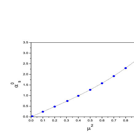
Figure 4: Dependence of IR fixed point $\alpha_{s}^{0}$ on the scaled quark mass $\mu^{2}=(m/\Lambda)^{2}$ at fixed confinement scale $\Lambda=345$ MeV.

Note that a value of $\hat{\alpha}_{s}^{0}$ of order  $2$ or larger would be definitely out of line with many other phenomena, such as nonrelativistic potentials for charmonium [59] and analytic perturbation theory [58]. Obviously, this constraint implies an upper limit to the value of constituent quark mass: $\mu^{2}<0.8$ or $m<0.9\,\Lambda$.

Since we are searching the IR-fixed point, it is reasonable to choose the lightest quark mass. Particularly, for $m=m_{ud}=192.56~{}\mbox{\rm MeV}$ and $\Lambda=345~{}\mbox{\rm MeV}$ we obtain

$$\hat{\alpha}_{s}^{0}=0.757\,,\qquad\mbox{or}\qquad{\hat{\alpha}_{s}^{0}/\pi}=0.241\,.$$ (20)

To compare our result with known data on $\alpha_{s}(Q)$ we exploit the integral relationships between the QCD running coupling in Euclidean and Minkowskian domains. Particularly, there exists a relation [16]

$$\alpha_{s}(q^{2})=q^{2}\int\limits_{0}^{\infty}{ds\over(s+q^{2})^{2}}\,\hat{\alpha}_{s}(s)$$ (21)

valid for the case of massless pion. By substituting $s=t\,q^{2}$ into (21) one rewrites

$$\alpha_{s}(q^{2})=\int\limits_{0}^{\infty}{dt\over(1+t)^{2}}\,\hat{\alpha}_{s}(t\,q^{2})\,.$$ (22)

Then, for $q^{2}\to 0$ we obtain

$$\alpha_{s}(0)=\hat{\alpha}_{s}(0)\int\limits_{0}^{\infty}{dt\over(1+t)^{2}}=\hat{\alpha}_{s}(0)\cdot 1\,.$$ (23)

Therefore, we may conclude that our result (20) is in reasonable agreement with often-quoted estimates

$$\left\{\begin{tabular}[]{l}${\alpha_{s}^{0}/\pi}\simeq 0.19-0.25$ \qquad\cite[cite]{[\@@bibref{}{godf85}{}{}]}\,,\\ ${\alpha_{s}^{0}/\pi}\simeq 0.265$ \qquad\qquad~{}~{}\cite[cite]{[\@@bibref{}{zhan91}{}{}]}\,,\\ ${\alpha_{s}^{0}/\pi}\simeq 0.26$ \qquad\qquad~{}~{}~{}\cite[cite]{[\@@bibref{}{halz93}{}{}]}\,,\\ $\left\langle{\alpha_{s}^{0}/\pi}\right\rangle_{1\,GeV}\simeq 0.2$ \qquad~{}~{}~{}\cite[cite]{[\@@bibref{}{doks96}{}{}]}\end{tabular}\right.$$ (24)

and phenomenological evidences [38, 31]. The obtained IR-fixed value of the coupling constant is moderate, it depends on the mass of constituent quark ($u,d$), so one can insert this value into perturbative expressions to be compatible with the experimental data.

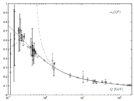
Figure 5: Summary of estimates of $\hat{\alpha}_{s}(M)$ in interval from 0 to 10 GeV at different values of confinement scale. In the left panel $\Lambda=330$ MeV (red dots), $\Lambda=345$ MeV (blue diamonds) and $\Lambda=360$ MeV (black squares) compared with $\alpha_{s}(Q)$ (in the right panel) defined in low-energy (open diamonds) and high-energy (open circles) experiments. Also shown are the three-loop analytic coupling (solid curve), its perturbative counterpart (dot-dashed curve) both normalized at the Z-boson mass, and the massive one-loop analytic coupling (dashed curve) (for details see Ref. [31]).

By interpolating smoothly obtained results in (20), (18) and (15) into the intermediate-energy region we define $\hat{\alpha}_{s}$ on a wide interval $0.14-9.5$ GeV. Some particular cases of the dependence $\alpha_{s}$ on mass scale $M$ at different model parameters are plotted in Fig. 5.

It is important to stress that we do not aim to obtain the behavior of the coupling constant at all scales. At moderate $M^{2}=-p^{2}$ we obtain $\alpha_{s}$ in coincidence with the QCD predictions. However, at large mass scale (above 10 GeV) $\hat{\alpha}_{s}$ decreases much faster than expected by QCD prediction. The reason is the use of confined propagators in the form of entire functions, Eqs. (2) and (3). Then, the convolution of entire functions leads to a rapid decreasing (or a rapid growth in Minkowski space) of physical matrix elements once the hadron masses and energies of the reaction have been fixed. Consequently, the numerical results become sensitive to changes of model parameters at large masses and energies.

4 Conclusion

To conclude, we provide an estimate of QCD effective charge in the low-energy region (below 1 GeV) by exploiting the conventional meson spectrum within a relativistic quantum-field model based on analytic (or infrared) confinement. The new results obtained in the previous section are summarized in Figs. 3-5 and Table 2.

We demonstrate that global properties of the low-energy phenomena such as QCD running coupling and conventional meson spectrum may be explained reasonably in the framework of a simple relativistic quantum-field model of quark-gluon interaction based on analytic (or, infrared) confinement. Our guess about the symmetry structure of the quark-gluon interaction in the confinement region has been tested and the use of simple forms of propagators has resulted in quantitatively reasonable estimates.

Despite its pure model origin, the approximations used, and questions about the very definition of the coupling in the IR region, our approach demonstrates a new, independent and specific IR-finite behavior of QCD coupling and we extract a particular IR-fixed point at $\hat{\alpha}_{s}(0)\simeq 0.757$ for confinement scale $\Lambda=345$ MeV. As an application, we performed estimates on intermediate and heavy meson masses and the result was in reasonable agreement with experimental data. Our estimates may be improved further by using iterative schemes, but the aim is to obtain a qualitative understanding of QCD effective coupling in the IR region.

The suggested model in its simple form is far from real QCD but we conclude that the analytic confinement conception combined with BS method may provide us with a rather satisfactory correlated understanding of low and intermediate-energy phenomena from few hundreds MeV to few GeV.

Note that further improvements of measurements of $\alpha_{s}$ will be difficult while it is unlikely that QCD perturbation theory will considerably improve existing predictions. Therefore, further developments of theoretical predictions within nonperturbative methods and reapplication of improved models may have successes in this field.

The author thanks M.A. Ivanov, E. Klempt and A.V. Nesterenko for useful discussions and valuable remarks.

References

- [1] M. Baldicchi and G.M. Prosperi, arXiv:0310213 [hep-ph] (2003).
- [2] Review of Particle Physics, C. Amsler et al., Phys. Lett. B667, 1 (2008).
- [3] C.T.H. Davies et al., HPQCD Collab., Phys.Rev. D78, 114507 (2008).
- [4] Yu. L. Dokshitzer, G. Marchesini and B. R. Webber, Nucl. Phys. B469, 93 (1996); Yu. L. Dokshitzer, V. A. Khoze and S. I. Troyan, Phys. Rev. D53, 89 (1996).
- [5] G. Corcella et al., JHEP 0101 , 010 (2001).
- [6] S. Chekanov et. al., Phys.Lett. B560, 7 (2003).
- [7] S. Bethke, J. Phys. G26, R27 (2000); arXiv:0004021 [hep-ex].
- [8] G.V. Efimov and G. Ganbold, Phys. Rev. D65, 054012 (2002).
- [9] G. Ganbold, AIP Conf. Proc. 717, 285 (2004); ibid 796, 127 (2005).
- [10] G. Ganbold, Phys. Rev. D79, 034034 (2009).
- [11] S. Bethke, Eur. Phys. J. C64, 689 (2009); arXiv:0908.1135 [hep-ph] (2009).
- [12] S. Bethke, Prog. Part. Nucl. Phys. 58, 351 (2007).
- [13] G. M. Prosperi, M. Raciti and C. Simolo, Prog. Part. Nuc. Phys. 58, 387 (2007); arXiv:hep-ph/0607209 [hep-ph] (2006).
- [14] A.V. Nesterenko and J.Papavassiliou, Phys. Rev. D71, 016009 (2005).
- [15] D.V. Shirkov, Theor. Math. Phys. 132, 1309 (2002).
- [16] A.V. Nesterenko, Int. J. M. Phys. A18, 5475 (2003).
- [17] O. Kaczmarek and F. Zantow, Phys. Rev. D71, 114510 (2005).
- [18] M.Beneke and M.Jamin, JHEP 0809, 044 (2008);
- [19] S.Narison, Phys. Lett. B673, 30 (2009);
- [20] M.Davier et al., Eur. Phys. J. C56, 305 (2008);
- [21] C. Davies et al., Nucl. Phys. Proc. Suppl. 119, 595 (2003).
- [22] A. Penin and A.A. Pivovarov, Phys. Lett. B435, 413 (1998).
- [23] P.A. Movilla Fernandez, arXiv:0205014 [hep-ex] (2002).
- [24] A. C. Mattingly and P. M. Stevenson, Phys. Rev. D49, 437 (1994).
- [25] A. C. Aguilar, A. Mihara and A. A. Natale, Phys. Rev. D65, 054011 (2002).
- [26] J. C. R. Bloch, Phys. Rev. D66, 034032 (2002).
- [27] D. Zwanziger, Phys. Rev. D65, 094039 (2002).
- [28] S. Capitani et. al., Nucl. Phys. B544, 669 (1999).
- [29] A. Sternbeck et. al., PoS LAT2007 (2007) 256; arXiv:0710.2965 [hep-lat] (2007).
- [30] P. Boucaud et al., Phys. Rev. D70, 114503 (2004).
- [31] M. Baldicchi, A.V. Nesterenko, G.M. Prosperi, D.V. Shirkov and G. Simolo, Phys. Rev. D77, 034013 (2008); arXiv:0705.1695v1 [hep-ph] (2007).
- [32] W. Buchmuller, G. Grunberg and S.-H. H. Tye, Phys. Rev. Lett. 45, 103 (1980); Phys. Rev. Lett. 45, 587 (1980).
- [33] M. Peter, Phys. Rev. Lett. 78, 602 (1997); Y. Schroder, Phys. Lett. B447, 321 (1999).
- [34] N. Brambilla, A. Pineda, J. Soto and A. Vairo, Phys. Rev. D60, 091502 (R) (1999); Nucl. Phys. B566, 275 (2000).
- [35] M. Baker, J. S. Ball, N. Brambilla, G.M. Prosperi, F. Zachariasen, Phys. Rev. D54, 2829 (1996).
- [36] S. Godfrey and N. Isgur, Phys. Rev. D32, 189 (1985); T. Barnes, F. E. Close and S. Monaghan, Nucl. Phys. B198, 380 (1983).
- [37] T. Zhang and R. Koniuk, Phys. Lett. B261, 311 (1991); C.R. Ji, F. Amiri, Phys. Rev. D42, 3764 (1990).
- [38] M. Baldicchi and G. M. Prosperi, AIP Conf. Proc. 756, 152 (2005); M. Baldicchi and G. M. Prosperi, Phys. Rev. D66, 074008 (2002).
- [39] F. Halzen, G. I. Krein and A. A. Natale, Phys. Rev. D47, 295 (1993).
- [40] H. Leutwyler, Phys. Lett. 96B, 154 (1980); Nucl. Phys. B179, 129 (1981).
- [41] E. Elizalde and J.Soto, Nucl. Phys. B260, 136 (1985).
- [42] G.V. Efimov and S.N. Nedelko, Phys. Rev. D51, 176 (1995); J.V. Burdanov, G.V. Efimov, S.N. Nedelko, S.A. Solunin, Phys. Rev. D54, 4483 (1996); J.V. Burdanov and G.V. Efimov, Phys. Rev. D64, 014001 (2001).
- [43] G. Ganbold, PoS Confinement8, 085, (2008).
- [44] D. Ebert, T.Feldmann and H.Reinhardt, Phys. Lett. B388, 154 (1996).
- [45] M.K.Volkov and V.L.Yudichev, Phys. Atom. Nucl. 63, 464 (2000).
- [46] E.E. Salpeter and H.A. Bethe, Phys. Rev. 84, 1232 (1951).
- [47] C. D. Roberts and A. G. Williams, Prog. Part. Nucl. Phys. 33, 477 (1994).
- [48] A. C. Aguilar, D. Binosi, J. Papavassiliou, J. Rodriguez-Quintero, Phys. Rev. D80, 085018 (2009).
- [49] T. Feldman, Int. J. Mod. Phys. A15, (2000) 159.
- [50] C. S. Fischer, R. Alkofer and H. Reinhardt, Phys. Rev. D65, 094008 (2002); C. S. Fischer and R. Alkofer, Phys. Lett. B536, 177 (2002),
- [51] C. Lerche and L. von Smekal, Phys. Rev. D65, 125006 (2002).
- [52] B. Alles et al., Nucl. Phys. B502, 325 (1997).
- [53] H. Gies, Phys.Rev. D66, 025006 (2002).
- [54] K. Langfeld, H. Reinhardt and J. Gattnar, Nucl. Phys. B621, 131 (2002).
- [55] K.A. Milton and I.L. Solovtsov, Phys. Rev. D55, 5295 (1997); D59, 107701 (1999).
- [56] S. J. Brodsky and G. F. de Teramond, Phys. Lett. B582, 211 (2004).
- [57] A. C. Aguilar, A. Mihara and A. A. Natale, Int. J. Mod. Phys. A19, 249 (2004).
- [58] D. V. Shirkov and I. L. Solovtsov, Phys. Rev. Lett. 79, 1209 (1997); D. V. Shirkov, Theor. Math. Phys. 136, 893 (2003); arXiv:0210013 [hep-th] (2002).
- [59] A. M. Badalian and B. L. G. Bakker, Phys. Rev. D62, 094031 (2000).