The $B\to D_{s}^{(*)}\pi$ decays in the perturbative QCD

Abstract

In this paper, we calculate the branching ratios for $B^{0}\to D_{s}^{+}\pi^{-},B^{+}\to D_{s}^{+}\pi^{0}$, $B^{0}\to D_{s}^{*+}\pi^{-}$ and $B^{+}\to D_{s}^{*+}\pi^{0}$ decays in the perturbative QCD factorization approach. We find that the calculated branching ratios of these four decay channels agree well with the measured values and current experimental upper limit. In the numerical calculation, we take the decay constant and the shape parameter of the vector meson $D^{*}_{s}$ as $f_{D^{*}_{s}}=312$ MeV and $a_{D^{*}_{s}}=0.78$ respectively, which are larger than those in the previous calculations.

I Introduction

In recent years, more and more effort has been made to the B meson decays with one cdlv1 even two cdlv2 charmed mesons in the final states and it is found that the perturbative QCD factorization (pQCD) approach does work well in these decays. We will calculate the branching ratios for the $B\to D^{(*)}_{s}\pi$ decays, which are shown in figure 1, by employing the pQCD approach. The momenta of the two outgoing mesons are both approximately $\frac{1}{2}m_{B}(1-m^{2}_{D^{(*)}_{s}}/m_{B}^{2})$. This is still large enough to make a hard intermediate gluon in the hard part calculation. Most of the momenta come from the heavy b quark in quark level. The light quark u (d) inside $B^{+}$ $(B^{0})$ meson, which is usually called spectator quark, carries small momentum of order of $\Lambda_{QCD}$. In order to form a fast moving light meson, the spectator quark need to connect the four-quark operator $(\bar{b}u)_{V-A}(\bar{c}s)_{V-A}$ through an energetic gluon. The hard four-quark dynamic together with the spectator quark becomes six-quark effective interaction. Since six-quark interaction is hard dynamics, it is perturbatively calculable in theory.

On the experimental side, the branching ratios of $B^{0}\to D_{s}^{+}\pi^{-},B^{+}\to D_{s}^{+}\pi^{0}$ and $B^{0}\to D_{s}^{*+}\pi^{-}$ have been measured by BaBar barbar1 and Belle belle . For $B^{+}\to D_{s}^{*+}\pi^{0}$ decay, only the experimental limit is given by CLEO cleo0 . We list their values in the following pdg08 :

$$Br(B^{0}\to D_{s}^{+}\pi^{-}) = (1.53\pm 0.35)\times 10^{-5},$$

$$Br(B^{+}\to D_{s}^{+}\pi^{0}) = (1.6\pm 0.6)\times 10^{-5},$$

$$Br(B^{0}\to D_{s}^{*+}\pi^{-}) = (3.0\pm 0.7)\times 10^{-5},$$

$$Br(B^{+}\to D_{s}^{*+}\pi^{0}) < 2.7\times 10^{-4}.$$ (1)

This paper is organized as follows. In Sect.II, the light-cone wave functions of the initial and the final state mesons are discussed. In Sec.III, we calculate analytically the related Feynman diagrams and present the various decay amplitudes for the studied decay modes. The numerical results and the discussions are given in the section IV. The conclusions are presented in the final part.

II Wave functions of initial and final state mesons

In pQCD calculation, the light-cone wave functions are nonperturbative and not calculable, but they are universal and channel independent for all the hadronic decays.

As a heavy meson, the B meson wave function is not well defined. In general, the B meson light-cone matrix element can be decomposed as grozin

$$\int_{0}^{1}\frac{d^{4}z}{(2\pi)^{4}}e^{i\bf{k_{1}}\cdot z}\langle 0|\bar{b}_{\alpha}(0)d_{\beta}(z)|B(p_{B})\rangle$$ (2)

$$= -\frac{i}{\sqrt{2N_{c}}}\left\{(P/_{B}+m_{B})\gamma_{5}\left[\phi_{B}({\bf k_{1}})-\frac{n/-v/}{\sqrt{2}}\bar{\phi}_{B}({\bf k_{1}})\right]\right\}_{\beta\alpha},$$

where $n=(1,0,{\bf 0_{T}})$, and $v=(0,1,{\bf 0_{T}})$ are the unit vectors pointing to the plus and minus directions, respectively. Because the contribution of the second Lorentz structure $\bar{\phi}_{B}(x,b)$ is numerically small and can be neglected, we only consider the contribution of the Lorentz structure:

$$\Phi_{B}(x,b)=\frac{1}{\sqrt{2N_{c}}}(P/_{B}+m_{B})\gamma_{5}\phi_{B}(x,b).$$ (3)

.

In the heavy quark limit, we take the wave functions for the pseudoscalar meson $D_{s}$ and the vector meson $D^{*}_{s}$ as

$$\Phi_{D_{S}}(x,b)=\frac{1}{\sqrt{2N_{c}}}\gamma_{5}(P/_{D_{s}}+m_{D_{s}})\phi_{D_{s}}(x,b),$$ (4)

$$\Phi_{D^{*}_{s}}(x,b)=\frac{1}{\sqrt{2N_{c}}}\epsilon/\,(P/_{D^{*}_{s}}+m_{D^{*}_{s}})\phi_{D^{*}_{s}}(x,b),$$ (5)

where the polar vector $\epsilon/\,=\frac{M_{B}}{\sqrt{2}M_{D^{*}_{s}}}(1,-r^{2}_{D^{*}_{s}},{\bf 0_{T}})$. In the considered decays, the $D^{*}_{s}$ meson is longitudinally polarized, so we only need to consider its wave function in longitudinal polarization.

The wave function for the light pseudoscalar meson $\pi$ is given as

$$\Phi_{\pi}(P,x,\zeta)\equiv\frac{1}{\sqrt{2N_{C}}}\gamma_{5}\left[P/\phi_{\pi}^{A}(x)+m_{0}^{\pi}\phi_{\pi}^{P}(x)+\zeta m_{0}^{\pi}(v/n/-v\cdot n)\phi_{\pi}^{T}(x)\right],$$ (6)

where $P$ and $x$ are the momentum and the momentum fraction of $\pi$ meson, respectively. The parameter $\zeta$ is either $+1$ or $-1$ depending on the assignment of the momentum fraction $x$. The chiral scale parameter $m_{0}^{\pi}$ is defined as $m_{0}^{\pi}=m^{2}_{\pi}/(m_{u}+m_{d})$.

III the perturbative QCD calculation

Using factorization theorem, we can separate the decay amplitude into soft, hard, and harder dynamics characterized by different scales, conceptually expressed as the convolution,

$${\cal A}(B\to D^{(*)}_{s}\pi)\sim\int\!\!d^{4}k_{1}d^{4}k_{2}d^{4}k_{3}\ \mathrm{Tr}\left[C(t)\Phi_{B}(k_{1})\Phi_{D^{(*)}_{s}}(k_{2})\Phi_{\pi}(k_{3})H(k_{1},k_{2},k_{3},t)\right],$$ (7)

where $k_{i}$’s are momenta of light anti-quarks included in each meson, and $\mathrm{Tr}$ denotes the trace over Dirac and color indices. $C(t)$ is the Wilson coefficient which results from the radiative corrections at a short distance. In the above convolution, $C(t)$ includes the harder dynamics at a larger scale than that at the $M_{B}$ scale and describes the evolution of local $4$-Fermi operators from $m_{W}$ (the $W$ boson mass) down to $t\sim\mathcal{O}(\sqrt{\bar{\Lambda}M_{B}})$ scale, where $\bar{\Lambda}\equiv M_{B}-m_{b}$. The function $H(k_{1},k_{2},k_{3},t)$ describes the four quark operator and the spectator quark connected by a hard gluon whose $q^{2}$ is in the order of $\bar{\Lambda}M_{B}$, and includes the $\mathcal{O}(\sqrt{\bar{\Lambda}M_{B}})$ hard dynamics. Therefore, this hard part $H$ can be perturbatively calculated. The function $\Phi_{(D^{(*)}_{s},\pi)}$ are the wave functions of $D^{(*)}_{s}$ and $\pi$.

Since the $b$ quark is rather heavy, we consider the B meson at rest for simplicity. It is convenient to use the light-cone coordinate $(p^{+},p^{-},{\bf p}_{T})$ is used to describe the meson’s momenta:

$$p^{\pm}=\frac{1}{\sqrt{2}}(p^{0}\pm p^{3}),\quad{\rm and}\quad{\bf p}_{T}=(p^{1},p^{2}).$$ (8)

At the rest frame of $B$ meson, the light meson moves very fast and so $P_{3}^{+}$ or $P_{3}^{-}$ can be treated as zero. Using these coordinates, the B meson and the two final state meson momenta can be written as

$$P_{B}=\frac{M_{B}}{\sqrt{2}}(1,1,{\bf 0}_{T}),\quad P_{2}=\frac{M_{B}}{\sqrt{2}}(1,r^{2},{\bf 0}_{T}),\quad P_{3}=\frac{M_{B}}{\sqrt{2}}(0,1-r^{2},{\bf 0}_{T}),$$ (9)

respectively, where $r=M_{D^{(*)}_{s}}/M_{B}$. Putting the light anti-quark momenta in $B$, $D^{(*)}_{s}$ and $\pi$ mesons as $k_{1}$, $k_{2}$, and $k_{3}$, respectively, we can choose

$$k_{1}=(x_{1}P_{1}^{+},0,{\bf k}_{1T}),\quad k_{2}=(x_{2}P_{2}^{+},0,{\bf k}_{2T}),\quad k_{3}=(0,x_{3}P_{3}^{-},{\bf k}_{3T}).$$ (10)

For these considered decay channels, the integration over $k_{1}^{-}$, $k_{2}^{-}$, and $k_{3}^{+}$ in equation (7) will lead to

$${\cal A}(B\to D^{(*)}_{s}\pi) \sim \int\!\!dx_{1}dx_{2}dx_{3}b_{1}db_{1}b_{2}db_{2}b_{3}db_{3}$$ (11)

$$\cdot\mathrm{Tr}\left[C(t)\Phi_{B}(x_{1},b_{1})\Phi_{D^{(*)}_{s}}(x_{2},b_{2})\Phi_{\pi}(x_{3},b_{3})H(x_{i},b_{i},t)S_{t}(x_{i})\,e^{-S(t)}\right],\quad\;$$

where $b_{i}$ is the conjugate space coordinate of $k_{iT}$, and $t$ is the largest energy scale in the function $H(x_{i},b_{i},t)$. The last term $e^{-S(t)}$ in equation (11) is the Sudakov form factor which suppresses the soft dynamics effectively soft .

Figure 1: Diagrams contributing to the decays $B\to D^{(*)}_{s}\pi$.

For the considered decays, the related weak effective Hamiltonian $H_{eff}$ can be written as buras96

$${\cal H}_{eff}=\frac{G_{F}}{\sqrt{2}}\,V_{ub}^{*}V_{cs}\left[\left(C_{1}(\mu)O_{1}(\mu)+C_{2}(\mu)O_{2}(\mu)\right)\right],$$ (12)

where the four-quark operators are

$$O_{1}=(\bar{b}_{\alpha}u_{\beta})_{V-A}(\bar{c}_{\alpha}s_{\beta})_{V-A},\quad O_{2}=(\bar{b}_{\alpha}u_{\alpha})_{V-A}(\bar{c}_{\alpha}s_{\alpha})_{V-A},$$ (13)

with $\alpha,\beta$ being the color indexes, and $(\bar{q}_{1}q_{2})_{V-A}=\bar{q}_{1}\gamma^{\mu}(1-\gamma^{5})q_{2}$. The Fermi constant $G_{F}=1.16639\times 10^{-5}GeV^{-2}$ and $C_{1,2}(\mu)$ are Wilson coefficients running with the renormalization scale $\mu$ . The leading order diagrams contributing to the decays $B\to D^{(*)}_{s}\pi$ are drawn in figure 1 according to this effective Hamiltonian.

In the following, we will get the analytic formulas by calculating the hard part $H(t)$ at leading order. Involving the meson wave functions, the amplitude for the factorizable tree emission diagrams Fig.1(a) and (b) can be written as:

$$F_{e} = 8\pi C_{F}f_{D^{(*)}_{s}}\int_{0}^{1}dx_{1}dx_{3}\int_{0}^{\infty}b_{1}db_{1}\,b_{3}db_{3}\,\Phi_{B}(x_{1},b_{1})$$ (14)

$$\times\left\{\left[(x_{3}+1)\phi^{A}_{\pi}(x_{3})-r_{\pi}(2x_{3}-1)(\phi^{P}_{\pi}(x_{3})+\phi^{T}_{\pi}(x_{3}))\right]\right.$$

$$\left.\times E_{e}(t)h_{e}(x_{1},x_{3}(1-r^{2}_{D^{(*)}_{s}}),b_{1},b_{3})S_{t}(x_{3})\right.$$

$$\left.+2r_{\pi}\phi^{P}_{\pi}(x_{3})E_{e}(t^{\prime})h_{e}(x_{3},x_{1}(1-r^{2}_{D^{(*)}_{s}}),b_{3},b_{1})S_{t}(x_{1})\right\}\;,$$

where $C_{F}=4/3$ is the group factor of $SU(3)_{c}$ gauge group, and the mass ratios $r_{\pi}=m_{0}^{\pi}/m_{B},r_{D^{(*)}_{s}}=m_{D^{(*)}_{s}}/m_{B}$. Here $f_{D^{(*)}_{s}}$ is the decay constant of $D^{(*)}_{s}$ meson, and $S_{t}(x)$ is the jet function PQCD . The factor evolving with the scale $t$ is given by:

$$E_{e}(t)=\alpha_{s}(t)\exp[-S_{B}(t)-S_{\pi}(t)],$$ (15)

where $S_{B}(t),S_{\pi}(t)$ are expressions for Sudakov form factors PQCD . The hard function is written as

$$h_{e}(x_{1},x_{2},b_{1},b_{2}) = K_{0}\left(\sqrt{x_{1}x_{2}}m_{B}b_{1}\right)\left[\theta(b_{1}-b_{2})K_{0}\left(\sqrt{x_{2}}m_{B}b_{1}\right)I_{0}\left(\sqrt{x_{2}}m_{B}b_{2}\right)\right.$$ (16)

$$\;\left.+\theta(b_{2}-b_{1})K_{0}\left(\sqrt{x_{2}}m_{B}b_{2}\right)I_{0}\left(\sqrt{x_{2}}m_{B}b_{1}\right)\right].$$

The hard scales $t^{(\prime)}$ in Eq.(14) are determined by

$$t = max(\sqrt{x_{3}(1-r^{2}_{D^{(*)}_{s}})}m_{B},1/b_{1},1/b_{3}),$$

$$t^{\prime} = max(\sqrt{x_{1}(1-r^{2}_{D^{(*)}_{s}})}m_{B},1/b_{1},1/b_{3}).$$ (17)

For the nonfactorizable tree emission diagrams Fig.1(c) and (d), all three meson wave functions are involved. The integraton of $b_{3}$ can be performed using $\delta$ function $\delta(b_{3}-b_{2})$ and the result is

$$M_{e} = -16\pi\sqrt{2N_{c}}C_{F}\int_{0}^{1}dx_{1}dx_{2}dx_{3}\int_{0}^{\infty}b_{1}db_{1}\,b_{2}db_{2}\,\Phi_{B}(x_{1},b_{1})\Phi_{D^{(*)}_{s}}(x_{2})$$ (18)

$$\times\left\{\left[(x_{2}-1)\phi^{A}_{\pi}(x_{3})+r_{\pi}x_{3}(\phi^{P}_{\pi}(x_{3})-\phi^{T}_{\pi}(x_{3}))\right]E_{n}(t)h^{1}_{n}(x_{1},x_{2},x_{3},b_{1},b_{2})\right.$$

$$\left.+[(x_{3}+x_{2})\phi^{A}_{\pi}(x_{3})-r_{\pi}x_{3}(\phi^{P}_{\pi}(x_{3})+\phi^{T}_{\pi}(x_{3}))E_{n}(t^{\prime})h^{2}_{n}(x_{1},x_{2},x_{3},b_{1},b_{2})]\right\},$$

where the expressions for the evolution factor is $E_{n}=\alpha_{s}(t)\exp[-S(t)|_{b_{3}=b_{1}}]$ with the Sudakov exponent $S=S_{B}+S_{D^{(*)}_{s}}+S_{\pi}$.

The hard functions $h^{i}_{n},i=1,2$ in the amplitude are given as

$$h^{i}_{n} = [\theta(b_{1}-b_{2})K_{0}(Ab_{1})I_{0}(Ab_{2})+\theta(b_{2}-b_{1})K_{0}(Ab_{2})I_{0}(Ab_{1})]$$ (19)

$$\times\left(\begin{matrix}\frac{\pi i}{2}\mathrm{H}_{0}(\sqrt{|G^{2}_{i}|}b_{3}),&\text{for}\quad G^{2}_{i}<0\\ \mathrm{K}_{0}(G_{i}b_{2}),&\text{for}\quad G^{2}_{i}>0\end{matrix}\right),$$

with the variables

$$A^{2} = x_{1}x_{3}(1-r^{2}_{D^{(*)}_{s}})m^{2}_{B},$$

$$G^{2}_{1} = (x_{1}+x_{2})r^{2}_{D^{(*)}_{s}}-(1-x_{1}-x_{2})x_{3}(1-r^{2}_{D^{(*)}_{s}})m^{2}_{B},$$

$$G^{2}_{2} = (x_{1}-x_{2})x_{3}(1-r^{2}_{D^{(*)}_{s}})m^{2}_{B}.$$ (20)

The hard scales in Eq.(19) are given by

$$t = max(Am_{B},\sqrt{G^{2}_{1}}m_{B},1/b_{1},1/b_{2}),$$

$$t^{\prime} = max(Am_{B},\sqrt{G^{2}_{2}}m_{B},1/b_{1},1/b_{2}).$$ (21)

Then the total decay amplitude of $B\to D^{(*)}_{s}\pi$ decays can be written as

$${\cal A}(B\to D^{(*)}_{s}\pi)=V_{ub}^{*}V_{cs}[F_{e}(C_{2}+\frac{C_{1}}{3})+M_{e}C_{1}].$$ (22)

IV Numerical results and discussions

Table 1: Input parameters used in the numerical calculationpdg08 ; cleo .

Masses	$m_{\pi}=0.14\mbox{ GeV}$,	$m_{0}^{\pi}=1.3\mbox{ GeV}$,
	$m_{D_{s}}=1.9685\mbox{ GeV}$,	$m_{D^{*}_{s}}=2.1123\mbox{ GeV}$,
	$m_{B}=5.28\mbox{ GeV}$,	$m_{W}=80.4\mbox{ GeV}$,
Decay constants	$f_{B}=0.19\mbox{ GeV}$,	$f_{\pi}=0.13\mbox{ GeV}$,
	$f_{D_{s}}=0.273\mbox{ GeV}$,	$f_{D^{*}_{s}}=0.312\mbox{ GeV}$,
Lifetimes	$\tau_{B^{\pm}}=1.638\times 10^{-12}\mbox{ s}$,	$\tau_{B^{0}}=1.530\times 10^{-12}\mbox{ s}$,
$CKM$	$V_{cb}=0.0412\pm 0.0011$,	$V_{us}=0.2255\pm 0.0019$.

For the numerical calculation, we list the input parameters in Table 1.

For the $B$ meson wave function, we adopt the model

$$\phi_{B}(x,b) = N_{B}x^{2}(1-x)^{2}\mathrm{exp}\left[-\frac{M_{B}^{2}\ x^{2}}{2\omega_{b}^{2}}-\frac{1}{2}(\omega_{b}b)^{2}\right],$$ (23)

where $\omega_{b}$ is a free parameter and we take $\omega_{b}=0.4\pm 0.04$ GeV in numerical calculations, and $N_{B}=91.745$ is the normalization factor for $\omega_{b}=0.4$.

For $D^{(*)}_{s}$ meson, the distribution amplitude is taken as:

$$\phi_{D^{(*)}_{s}}(x)=f_{D^{(*)}_{s}}\frac{1}{\sqrt{6}}x(1-x)\left[1-a_{D^{(*)}_{s}}(1-2x)\right],$$ (24)

with the Gegenbauer coefficients $a_{D_{s}}=0.3$ and $a_{D^{*}_{s}}=0.78$. The CLEO and BarBar collaborations reported their work on the measurements of the decay constant of $D_{s}$ meson and obtained $f_{D_{s}}=274\pm 13\pm 7$ MeV cleo and $283\pm 17\pm 7\pm 14$ MeV barbar , respectively. However, the decay constant of the vector meson $D^{*}_{s}$ has not been directly measured in experiments so far. From the conclusions draw by the CLEO collaboration cleo , one can find that there exists a relation:

$$\frac{f_{D^{*}_{s}}}{f_{D^{*}}}\approx\frac{f_{D_{s}}}{f_{D}}\approx\frac{f_{B_{s}}}{f_{B}}=[1.1,1.2],$$ (25)

which is consistent with that from lattice simulation ukqcd and the QCD sum rules calculations yuming . From table 1, it is easy to see the value of the ratio $f_{D^{*}_{s}}/f_{D_{s}}$ is $1.14$ in our work. It is different from runhui , where the relation between $f_{D^{*}_{s}}$ and $f_{D_{s}}$ derived from HQET

$$\frac{f_{D^{*}_{s}}}{f_{D_{s}}}=\sqrt{\frac{m_{D_{s}}}{m_{D^{*}_{s}}}},$$ (26)

was used. From this equation, one can get the value of $f_{D^{*}_{s}}$, which is smaller than that of $f_{D_{s}}$.

The twist-2 pion distribution amplitude $\phi^{A}_{\pi}$, and the twist-3 ones $\phi^{P}_{\pi}$ and $\phi^{T}_{\pi}$ have been parametrized as

$$\phi_{\pi}^{A}(x) = \frac{f_{\pi}}{2\sqrt{2N_{c}}}6x(1-x)\left[1+a_{1}^{\pi}C^{3/2}_{1}(2x-1)+a^{\pi}_{2}C^{3/2}_{2}(2x-1)\right.$$ (27)

$$\left.+a^{\pi}_{4}C^{3/2}_{4}(2x-1)\right],$$

$$\phi_{\pi}^{P}(x) = \frac{f_{\pi}}{2\sqrt{2N_{c}}}\left[1+(30\eta_{3}-\frac{5}{2}\rho^{2}_{\pi})C^{1/2}_{2}(2x-1)-3\left\{\eta_{3}\omega_{3}+\frac{9}{20}\rho^{2}_{\pi}(1+6a^{\pi}_{2})\right\}\right.$$ (28)

$$\left.\times C^{1/2}_{4}(2x-1)\right],$$

$$\phi_{\pi}^{T}(x) = \frac{f_{\pi}}{2\sqrt{2N_{c}}}(1-2x)\left[1+6(5\eta_{3}-\frac{1}{2}\eta_{3}\omega_{3}-\frac{7}{20}\rho^{2}_{\pi}-\frac{3}{5}\rho^{2}_{\pi}a_{2}^{\pi})(1-10x+10x^{2})\right],\quad\quad$$ (29)

with the mass ratio $\rho_{\pi}=(m_{u}+m_{d})/m_{\pi}=m_{\pi}/m_{0}^{\pi}$ and the Gegenbauer polynomials $C^{\nu}_{n}(t)$,

$$C^{1/2}_{2}(t) = \frac{1}{2}(3t^{2}-1),\qquad C^{1/2}_{4}(t)=\frac{1}{8}(3-30t^{2}+35t^{4}),$$ (30)

$$C^{3/2}_{1}(t) = 3t,\qquad C^{3/2}_{2}(t)=\frac{3}{2}(5t^{2}-1),$$ (31)

$$C^{3/2}_{4}(t) = \frac{15}{8}(1-14t^{2}+21t^{4}).$$ (32)

The Gegenbauer coefficients are given as

$$a^{\pi}_{1}=0,\quad a^{\pi}_{2}=0.115,\quad a^{\pi}_{4}=-0.015.$$ (33)

The values of other parameters are taken as bf $\eta_{3}=0.015$ and $\omega=-3.0$.

In the B-rest frame, the decay width of $B\to D^{(*)}_{s}\pi$ can be obtained by

$$\Gamma=\frac{1}{32\pi}G_{F}^{2}m^{7}_{B}|{\cal A}|^{2}(1-r^{2}_{D^{(*)}_{s}}),$$ (34)

where ${\cal A}$ is the total decay amplitude shown in Eq.(22).

Table 2: Branching ratios ($\times 10^{-5}$) for the decays $B^{0}\to D_{s}^{+}\pi^{-},D_{s}^{*+}\pi^{-}$ and $B^{+}\to D_{s}^{+}\pi^{0},D_{s}^{*+}\pi^{0}$. The first theoretical error is from the the B meson shape parameter $\omega_{b}$. The second error is from the higher order pQCD correction. The third one is from the uncertainties of CKM matrix elements.

Channel	This work	Data
$B^{0}\to D_{s}^{+}\pi^{-}$	$1.85^{+0.36+0.41+0.10}_{-0.52-0.56-0.10}$	$1.53\pm 0.35$
$B^{+}\to D_{s}^{+}\pi^{0}$	$1.98^{+0.39+0.81+0.11}_{-0.56-0.31-0.11}$	$1.6\pm 0.6$
$B^{0}\to D_{s}^{*+}\pi^{-}$	$2.59^{+0.45+0.70+0.15}_{-0.76-0.60-0.15}$	$3.0\pm 0.7$
$B^{+}\to D_{s}^{*+}\pi^{0}$	$2.78^{+0.48+0.74+0.16}_{-0.82-0.65-0.16}$	$<27$

Using the wave functions as specified in the previous section and the input parameters listed in this section, it is straightforward to calculate the CP-averaged branching ratios for the considered decays, which are listed in Table 2. The first error in these entries is caused by the B meson shape parameter $\omega_{b}=0.40\pm 0.04$. The second error is from the higher order pQCD correction: the choice of hard scales, defined in Eq.(17) and Eq.(21), which vary from $0.9t$ to $1.1t$. The third error is from the uncertainties of the CKM matrix elements which are listed in table 1.

In previous calculations cdlv1 ; cdlv2 , the authors have considered that the value of the Gegenbauer moment $a_{D^{*}_{s}}$ was the same as that of $a_{D_{s}}$ and taken them as $0.3$. Here we take $a_{D^{*}_{s}}=0.78$, which is determined to fit the requirement that $\phi_{D^{*}_{s}}(x)$, shown in Eq.(24), has a maximum at $\bar{x}=\frac{m_{D_{s}}-m_{c}}{m_{D_{s}}}$. In Fig. 2, we plot that $a_{D^{*}_{s}}$ dependence of the branching ratios of $B^{0}\to D^{+*}_{s}\pi^{-}$ and $B^{+}\to D^{+*}_{s}\pi^{0}$. One can find that the branching ratios are not sensitive to the variations of $a_{D^{*}_{s}}$.

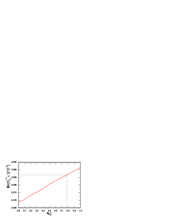
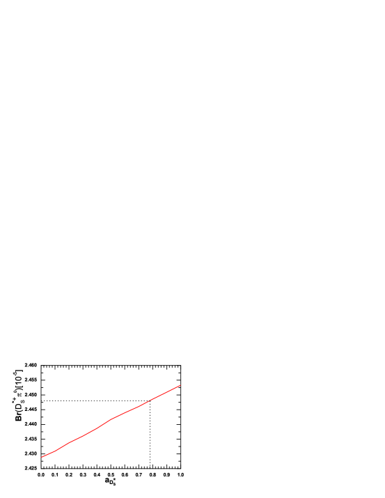
Figure 2: Branching ratios (in units of $10^{-5}$) of $B^{0}\to D_{s}^{*+}\pi^{-}$ and $B^{+}\to D_{s}^{*+}\pi^{0}$ decays as functions of Gegenbauer moment $a_{D^{*}_{s}}$ .

From the numerical results, we find that the non-factorizable contributions are very small and almost neglectable. They are about $10\%$ of the factorizable ones in each decays. The main contributions come from the factorizable amplitudes.

V Conclusion

In this paper, we calculate the branching ratios of decays $B^{0}\to D_{s}^{+}\pi^{-},B^{+}\to D_{s}^{+}\pi^{0}$, $B^{0}\to D_{s}^{*+}\pi^{-}$ and $B^{+}\to D_{s}^{*+}\pi^{0}$ in the pQCD factorization approach. We find that:

• The decays considered here have branching ratios about $10^{2}$ smaller than those of the $B\to D^{(*)}\pi$ decays, and they comes mainly from the relevant CKM matrix elements.

• From the numerical results shown in table 2, one can find that the pQCD predictions for these considered decay channels are consistent with the measured values and currently available experimental upper limit.

• To determine decay constant of the vector meson $D^{*+}_{s}$ , the relation

  $$\frac{f_{D^{*}_{s}}}{f_{D^{*}}}\approx\frac{f_{D_{s}}}{f_{D}}\approx\frac{f_{B_{s}}}{f_{B}}$$ (35)

  is used. It indicates that the value of $f_{D^{*}_{s}}$ is larger than that of $f_{D^{*}}$, which is contrary to the conclusion derived from the relation

  $$\frac{f_{D^{*}_{s}}}{f_{D_{s}}}=\sqrt{\frac{m_{D_{s}}}{m_{D^{*}_{s}}}}\;.$$ (36)

• In the numerical calculation, we take $a_{D^{*}_{s}}=0.78$, which is larger than the value given in the previous calculations. It is determined to fit the requirement that the wave function $\phi_{D^{*}_{s}}(x)$ has a maximum at $\bar{x}=\frac{m_{D_{s}}-m_{c}}{m_{D_{s}}}$.

References

• (1) C.D.Β LΓΌ and K.Β Ukai, Eur. Phys. J. C 28, 305 (2003); C.D.Β LΓΌ, Eur. Phys. J. C 24, 121 (2002); Phys. Rev. D 68, 097502 (2003); Y.Li and C.D.Β LΓΌ, J. Phys. G 29, 2115 (2003); Chin.Phys.C 27(2003).
• (2) Y.Β Li, C.D.Β LΓΌ and Z.J.Β Xiao, J. Phys. G 31,273 (2005); C.D.Β LΓΌ and G.L. Song, Phys. Lett. BΒ 562 (2003).
• (3) BaBar Collaboration, B.Β Aubert et al., Phys. Rev. Lett. 98, 081801 (2007); Phys. Rev. Lett. 98, 171801 (2007).
• (4) Belle Collaboration, P.Β Krokovny et al., Phys. Rev. Lett. 89, 231804 (2007).
• (5) CLEO Collaboration, J.Β Alexander et al., Phys. Lett. BΒ 319, 369 (1993).
• (6) Particle Data Group, C.Β Amsler et al., Phys. Lett. BΒ 667, 1 (2008).
• (7) A.G.Β Grozin and M.Β Neubert, Phys. Rev. DΒ 55 272 (1997); M.Β Beneke and T.Β Feldmann, Nucl.Phys.B 592 3 (2001).
• (8) H.N.Β Li and B.Β Tseng, Phys. Rev. DΒ 57, 443 (1998).
• (9) G.Β Buchalla , A.J.Β Buras , M.E.Β Lautenbacher, Rev. Mod. Phys. 68, 1125 (1996).
• (10) Y.Y.Β Keum , H.-n.Β Li, and A.I.Β Sanda, Phys. Lett. B 504, 6 (2001); Phys. Rev. DΒ 63, 054008 (2001); C.D.Β LΓΌ, K.Β Ukai and M.Z.Β Yang, Phys. Rev. DΒ 63, 074009 (2001).
• (11) CLEO Collaboration, M. Artuso et al., Phys. Rev. Lett. 95, 251801 (2005); CLEO Collaboration, M. Artuso et al., Phys. Rev. Lett.Β 99, 071802 (2007); CLEO Collaboration, T. K. Pedlar et al., Phys. Rev. DΒ 76 072002 (2007).
• (12) BABAR Collaboration, B. Aubert et al., Phys. Rev. Lett. 98, 141801 (2007).
• (13) UKQCD Collaboration, K. C. Bowler et al., Nucl. Phys. B 619, 507 (2001).
• (14) Y.M.Β Wang, et al., Eur.Phys. J. C 54, 107 (2008).
• (15) R.H.Β Li, C.D.Β LΓΌ and H.Β Zou, Phys. Rev. DΒ 78, 014018 (2008).
• (16) V.M.Β Braun and I.E.Β Filyanov, Z. Phys. C 48, 239 (1990).