Fast transfer and efficient coherent separation of bound cluster in the extended Hubbard model

Abstract

We study the formation and dynamics of the bound pair (BP) and bound triple (BT) in strongly correlated extended Hubbard model for both Bose and Fermi systems. We find that the bandwidths of the BP and BT gain significantly when the on-site and nearest-neighbor interaction strengths reach the corresponding resonant points. This allows the fast transfer and efficient coherent separation of the BP and BT. The exact result shows that the success probability of the coherent separation is unity in the optimal system. In Fermi system, this finding can be applied to create distant entanglement without the need of temporal control and measurement process.

I Introduction

Ultra-cold atoms have turned out to be an ideal playground for testing few-particle fundamental physics and for their increasing technological applications. The experimental observation of atomic bound pair (BP) in optical lattice Winkler stimulates many experimental and theoretical investigations in strongly correlated boson systems Mahajan ; Petrosyan ; Creffield ; Kuklov ; Folling ; Zollner ; ChenS ; Valiente ; JLBP ; MVExtendB ; MVTB . The essential physics of the proposed BP is that, the periodic potential suppresses the single particle tunneling across the barrier, a process that would lead to a decay of the pair. Such kind of BP therefore cannot get migration speed through the lattice. In addition, the dynamics of the pair separation and formation is also of interest in both fundamental and application aspects.

In this article we study the influence of the nearest-neighbor (NN) interaction on the few-boson bound state. We will show that, the resonant NN interaction can also induce the BP and bound triple (BT) states. These bound states are distinct from the known ones, as their bandwidths are comparable to that of a single particle. This feature allows the full overlap between the scattering band of a single particle and the band of a BP or a BT, leading to the coherent separation and combination processes. We propose relatively simple schemes to implement such processes. The exact result shows that the success probability of the coherent separation is unity for a BP while approaches to unity for a BT in the optimal systems. Applying the scheme to the extended Fermi-Hubbard system, the coherent separation process can be utilized to create long-distance entanglement without the need of temporal control and measurement process.

II Fast bound pair dynamics

Let us start by analyzing in detail the two-particle problem in an extended Bose-Hubbard model, which is simpler than the Fermi one but shares the similar features for the issue concerned. The Hamiltonian is written as follows:

$$H_{\text{B}}=-t\overset{N}{\sum_{i=1}}\left(a_{i}^{{\dagger}}a_{i+1}+\text{H.c.}\right)+\frac{U}{2}\overset{N}{\sum_{i=1}}n_{i}(n_{i}-1)+V\overset{N}{\sum_{i=1}}n_{i}n_{i+1},$$ (1)

where $a_{i}^{{\dagger}}$ is the creation operator of the boson at the $i$th site, the tunneling strength, on-site and NN interactions between bosons are denoted by $t$, $U$ and $V$. For the sake of clarity and simplicity, we only consider odd-site system with $N=2N_{0}+1$, and periodic boundary conditions $a_{N+1}=a_{1}$. In this article, we only concern the one-dimensional system. Nevertheless the conclusion can be extended to high-dimensional system.

First of all, a state in the two-particle Hilbert space, as shown in Ref. JLBP , can be written as $\left|\psi_{k}\right\rangle=$ $\sum_{k,r}f^{k}(r)\left|\phi_{r}^{k}\right\rangle,$ with

$$\left|\phi_{0}^{k}\right\rangle = \frac{1}{\sqrt{2N}}e^{i\frac{k}{2}}\sum_{j}e^{ikj}\left(a_{j}^{{\dagger}}\right)^{2}\left|\text{vac}\right\rangle,$$ (2)

$$\left|\phi_{r}^{k}\right\rangle = \frac{1}{\sqrt{N}}e^{i\frac{k(r+1)}{2}}\sum_{j}e^{ikj}a_{j}^{{\dagger}}a_{j+r}^{{\dagger}}\left|\text{vac}\right\rangle,$$ (3)

here $\left|\text{vac}\right\rangle$ is the vacuum state for the boson operator $a_{i}$. $k=2\pi n/N$, $n\in[1,N]$ denotes the momentum, and $r\in[1,N_{0}]$ is the distance between the two particles. Due to the translational symmetry of the present system, the Schrödinger equations for $f^{k}(r)$, $r\in[0,N_{0}]$ are easily shown to be

$$\begin{split}&T_{r}^{k}f^{k}(r+1)+T_{r-1}^{k}f^{k}(r-1)\\ &+[U\delta_{r,0}+V\delta_{r,1}+\left(-1\right)^{n}T_{r}^{k}\delta_{r,N_{0}}-\varepsilon_{k}]f^{k}(r)=0,\end{split}$$ (4)

where $T_{r}^{k}=-2\sqrt{2}t\cos(k/2)$ for $r=0$, and $-2t\cos(k/2)$ for $r\neq 0$, respectively. Besides, we also have the boundary conditions $f^{k}(-1)=$ $f^{k}(N_{0}+1)=0$. Note that for an arbitrary $k$, the solution of (4) is equivalent to that of the single-particle $N_{0}+1$-site tight-binding chain system with NN hopping amplitude $T_{j}^{k}$, on-site potentials $U$, $V$ and $-2t\cos(k/2)$ at $0$th, $1$th and $N_{0}$th sites respectively. Obviously, in each $k$-invariant subspace, there are three types of bound states arising from the on-site potentials under the following conditions. In the case with $\left|U-V\right|\gg t$, the particle can be localized at either $0$th or $1$th site, corresponding to (i) the on-site BP state, or (ii) the NN BP state. Interestingly, in the case of resonance $U=V$, and $\left|U\right|$, $\left|V\right|\gg t$, the particle can be in the bonding state (or anti-bonding state) between $0$th and $1$th sites, corresponding to a new BP state, called (iii) the resonant BP (RBP) state. In this article, hereafter we forcus on this type of bound state and refer RBP as BP. All the $N$ bound states of (iii), indexed by $k$, constitute a bound-pair band.

In previous works JLBP ; MVExtendB , the bound states of (i) and (ii) were well investigated and the corresponding bound-pair bandwidths are of $t^{2}/U$ and $t^{2}/V\$order. Then they can be regarded as stationary comparing to the single particle in the strongly correlated limit. In order to analyze the dynamics of the BP of type (iii), we pursue the solution of Eq. (4) in the case with $U=V$, and $\left|U\right|$, $\left|V\right|\gg t$, via the Bathe-ansatz method. The BP states have the form

$$f^{k}(r)\simeq\eta_{k}\left\{\begin{array}[]{c}-\sqrt{2}\epsilon_{k}/\left(\varepsilon_{k}-U\right)\text{,\ }(r=0),\\ \left[-\text{sgn}\left(U/\epsilon_{k}\right)\right]^{\left(r-1\right)}\left(\xi_{k}\right)^{-\left(r-1\right)}\text{,}\end{array}\right.$$ (5)

with the spectrum

$$\varepsilon_{k}\simeq U\pm\sqrt{2}\epsilon_{k}+\frac{\left(\epsilon_{k}\right)^{2}}{2U},$$ (6)

where

$$\eta_{k}^{-2} = \frac{\left|\varepsilon_{k}\right|}{2\sqrt{\varepsilon_{k}^{2}-4\left(\epsilon_{k}\right)^{2}}}+\frac{2\left(\epsilon_{k}\right)^{2}}{\left(\varepsilon_{k}-U\right)^{2}}+\frac{1}{2},$$ (7)

$$\xi_{k} = \left(\left|\varepsilon_{k}\right|+\sqrt{\varepsilon_{k}^{2}-4\left(\epsilon_{k}\right)^{2}}\right)/\left(2\left|\epsilon_{k}\right|\right),$$ (8)

and

$$\epsilon_{k}=-2t\cos\left(k/2\right),$$ (9)

is partial dispersion relation of a single particle. We note that neglecting the terms with $t^{2}/U$, the two branches of the spectrum combine into a BP band and the corresponding eigenfunction and energy can be rewritten as

$$\left|\psi_{k}^{\text{BP}}\right\rangle=\sum_{j}\frac{e^{ik\left(j+1/2\right)}}{\sqrt{2N}}\left[\left(a_{j}^{{\dagger}}\right)^{2}/\sqrt{2}\mp e^{i\frac{k}{2}}a_{j}^{{\dagger}}a_{j+1}^{{\dagger}}\right]\left|\text{vac}\right\rangle,$$ (10)

$$\varepsilon_{k}^{\text{BP}}=U\pm 2\sqrt{2}t\cos\left(k/2\right).$$ (11)

Observing the above expressions, we find that it can be regarded as a plane wave of the composite particle, BP. Actually, this can be easily understood in terms of the equivalent effective Hamiltonian, which can be obtained in the quasi-invariant subspace spanned by the basis $\{\underline{\left|l\right\rangle},l\in\left[1,2N\right]\}$ with diagonal energy $U$. The set of basis $\{\underline{\left|l\right\rangle}\}$ is defined as

$$\underline{\left|l\right\rangle}\equiv\left\{\begin{array}[]{c}\left(a_{l/2}^{{\dagger}}\right)^{2}/\sqrt{2}\left|\text{vac}\right\rangle\text{, }(\text{even }l)\\ a_{\left(l-1\right)/2}^{{\dagger}}a_{\left(l+1\right)/2}^{{\dagger}}\left|\text{vac}\right\rangle\text{,\ }(\text{odd }l)\end{array}\right.,$$ (12)

The effective Hamiltonian of the ring, restricted to the basis $\{\underline{\left|l\right\rangle}\}$ and shifted by $U$, reads

$$\mathcal{H}_{\text{BP}}=-\sqrt{2}t\overset{2N}{\sum_{l=1}}\left(\underline{\left|l\right\rangle}\underline{\left\langle l+1\right|}+\text{H.c.}\right),$$ (13)

which describes a free Bloch particle in a single band. However, this BP state is distinct from the previous on-site and NN BP because of its large bandwidth, $4\sqrt{2}t$. It shows that the speed of a BP wavepacket must be in the range of $0\sim 2\sqrt{2}t$, which is the reason why we call it fast bound pair. This is very significant for quantum technologies in the following two aspects: (i) The BP wavepacket can be a new candidate as quantum information carrier due to its fast speed. (ii) The bandwidth matching between BP and a single particle may lead to the coherent separation of the BP.

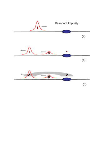
Figure 1: (Color online) Schematic illustration of the coherent separation process of a BP in the proposed optimal system. It consists of a uniform chain and the embedded resonant impurity. (a) An incident BP wavepacket comes from the left and scatters off the resonant impurity. (b) The reflected waves contain the BP and the single particle wavepackets with different speeds. A single particle resides at the impurity. For an optimal incident wavepacket, the success probability of the coherent separation is unity. (c) Appling the previous scheme to a singlet femionic BP, it is found that the separated two fermions are maximally entangled.

III Coherent separation of bound pair

Considering a system of (1) with the additional chemical potential $\mu=U$, the scattering band of a single particle fully overlaps the band of a BP (6). This fact indicates that a BP may break in the scattering process by a resonant impurity. In order to demonstrate a perfect process of the BP separation, we propose an optimal system which is a uniform chain with a resonant impurity embedded in. The uniform chain acts as a channel for the transport of a BP wave, under the conditions $U=V$, and $\left|U\right|$, $\left|V\right|\gg t$. The resonant impurity consists of two sites with the tunneling strength $t_{0}$, one site of which has far-off resonant on-site interaction $U_{s}$ satisfying $\left|U_{s}-U\right|\gg t$ and another site has resonant chemical potential $\mu=U$.

This setup is described by the Hamiltonian

$$H_{\text{BPS}}=-\left(t\overset{\infty}{\sum_{i=-\infty}}a_{i}^{{\dagger}}a_{i+1}+\left(t_{0}-t\right)a_{0}^{{\dagger}}a_{1}\right)+\text{H.c.}$$ (14)

$$+U\overset{\infty}{\sum_{i=-\infty}}n_{i}(\frac{n_{i}}{2}+n_{i+1}-1)+\frac{U_{s}-U}{2}n_{0}(n_{0}-1)+Un_{1}.$$

To investigate the scattering process of an input BP wavepacket from the left, one can establish an equivalent effective Hamiltonian in the quasi-invariant subspace spanned by the following basis $\{\underline{\left|l\right\rangle},l\in\left(-\infty,\infty\right)\}$ defined as

$$\underline{\left|l\right\rangle}\equiv\left\{\begin{array}[]{c}\text{Eqs. (\ref{BP_basis}), }(l<0)\\ a_{-l-1}^{{\dagger}}a_{1}^{{\dagger}}\left|\text{vac}\right\rangle\text{,\ }(l\geqslant 0)\end{array}\right..$$ (15)

Acting $H_{\text{BPS}}$ on the subspace, the equivalent effective Hamiltonian reads

$$\mathcal{H}_{\text{BPS}}=-t\left(\sqrt{2}\overset{-1}{\sum_{l=-\infty}}\overset{\infty}{+\sum_{l=1}}\right)\underline{\left|l-1\right\rangle}\underline{\left\langle l\right|}-t_{0}\underline{\left|-1\right\rangle}\underline{\left\langle 0\right|}+\text{H.c.}$$ (16)

which describes a two connected semi-infinite chains with different hopping constants. The on-site interaction $U_{s}$ ensures $H_{\text{BPS}}$ to be a linear chain, which would be of benefit to enhance the success probability of the coherent separation.

The separation process of a BP wavepacket is illustrated in Fig. 1. After scattering, a part of the BP wavepacket is reflected by the impurity, while the other part of it is separated into two independent particles: One of the particle resides at the site with chemical potential $U$, while the other particle is reflected to the left with higher speed than the reflected BP wavepacket. In the aid of the effective Hamiltonian (16), the previous process can be reduced to a simple single particle scattering problem: An incident wavepacket is scattered by the joint of the two semi-infinite chains. The reflecting wave represents the reflecting BP wave, while the transmitting wave represents the separated reflecting particle. In this sense, the coherent separation probability is equal to the transmission coefficient of the effective Hamiltonian, which can be obtained exactly via Green’ function or Bethe-ansatz method Datta ; YangAs ; JLTrans .

For an incident plane wave of $k_{0}$, the coherent separation probability $P\left(k_{0}\right)$ for a chosen system of $t_{0}=\sqrt[4]{2}t$ is

$$P\left(k_{0}\right)=2\left[1+\frac{1-\sqrt{2}\cos^{2}\left(k_{0}\right)}{\sin k_{0}\sqrt{\left|\cos\left(2k_{0}\right)\right|}}\right]^{-1},$$ (17)

for $k_{0}\in(\pi/4,\pi/2]$ and $P\left(k_{0}\right)=0$ for $k_{0}\in(0,\pi/4]$. The sudden death of $P\left(k_{0}\right)$ within the region $(0,\pi/4]$ is due to the mismatch between energies of the two sides of the joint. On the other hand,$\ P\left(k_{0}\right)$ also represents the particle resident population at the impurity. The profile of $P\left(k_{0}\right)$ is plotted in Fig. 2. It indicates that $P\left(k_{0}\right)$ can reach $1.0$ at $k_{0}=\pi/2$.

In practice, this process can be implemented via an incident wavepacket instead of a plane wave. Actually, the typical wavepacket, a Gaussian wave packet in the space $\{\underline{\left|l\right\rangle}\}$ can be constructed as

$$\left|\Phi(k_{0},N_{c})\right\rangle=\frac{1}{\sqrt{\Omega}}\sum_{l}e^{-\frac{{}^{\alpha^{2}}}{2}(l-N_{c})^{2}+ik_{0}l}\underline{\left|l\right\rangle},$$ (18)

where $\Omega$ is the normalization factor. Here $N_{c}$ is the center of it in the space $\{\underline{\left|l\right\rangle}\}$, $k_{0}$ is the momentum of it. The corresponding group velocity in the space $\{\underline{\left|l\right\rangle}\}$ is $v_{g}=-2\sqrt{2}t\sin\left(k_{0}\right)$ which is also plotted in Fig. 2. It shows that for the fastest wavepacket with momentum $\pm\pi/2$, the success probability of the coherent separation can approach to unity. In addition, it is shown that such a wavepacket is the most robust against spreading KimImpurity . We define it as the optimal BP wavepacket to demonstrate the perfect coherent separation. In the original system, it can be written as

$$\left|\phi(\pm,h_{c})\right\rangle \simeq \frac{1}{\sqrt{\Omega}}\sum_{j}\left(-1\right)^{j}e^{-2\alpha^{2}\left(j-h_{c}\right)^{2}}$$ (19)

$$\times\left[\left(a_{j}^{{\dagger}}\right)^{2}/\sqrt{2}\pm ia_{j}^{{\dagger}}a_{j+1}^{{\dagger}}\right]\left|\text{vac}\right\rangle,$$

which is obtained from (18) with wide width $\left(\alpha\ll 1\right)$ and $k_{0}=\pm\pi/2$ by the mapping rule (15). Here symbols $\pm$ and $h_{c}$ denote the moving direction (sgn$\left(\pm\pi/2\right)$) and the center of the wavepacket. The corresponding single particle wave packet has the form

$$\left|\varphi(\pm,h_{c})\right\rangle=\frac{1}{\sqrt{\Omega}}\sum_{j}e^{-\frac{{}^{\alpha^{2}}}{2}(j-h_{c})^{2}\pm i\frac{\pi}{2}j}a_{j}^{{\dagger}}\left|\text{vac}\right\rangle.$$ (20)

Note that $\left|\phi(\pm,h_{c})\right\rangle$ is narrower and slower than that of $\left|\varphi(\pm,h_{c})\right\rangle$. This is also illustrated in Fig. 1 (b) and (c).

Thus, in the optimal case, the perfect scattering process can be expressed as

$$\left|\phi(+,-\infty)\right\rangle\left|\text{vac}\right\rangle\Longrightarrow$$

$$r\left|\phi(-,-\infty)\right\rangle\left|\text{vac}\right\rangle+t\left|\varphi(-,-\infty)\right\rangle a_{1}^{{\dagger}}\left|\text{vac}\right\rangle,$$ (21)

and the corresponding inverse process as

$$\left|\varphi(+,-\infty)\right\rangle a_{1}^{{\dagger}}\left|\text{vac}\right\rangle\Longrightarrow$$

$$r\left|\varphi(-,-\infty)\right\rangle a_{1}^{{\dagger}}\left|\text{vac}\right\rangle+t\left|\phi(-,-\infty)\right\rangle\left|\text{vac}\right\rangle,$$ (22)

where $\Longrightarrow$ represents the time evolution. Eqs. (21) and (22) represent the reversibility of the processes, coherent separation and combination, due to the time-reversal symmetry of the system. Here $r$ and $t$ represent the reflection and transmission amplitudes. Then the success probability of the coherent separation is $\left|t\right|^{2}$. Numerical simulation is performed to evaluate the separation probability. For an optimal Gaussian wavepacket with $\alpha=0.01$, we have $\left|t\right|^{2}=1.00$. Hence we conclude that the coherent separation scheme is indeed very efficient due to its three advantages, fast transfer, robustness and high efficiency.

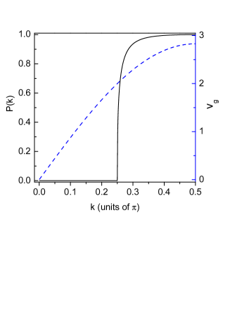
Figure 2: (Color online) Plots of the separation probability $P\left(k\right)$ (solid line) and the group velocity $v_{g}$ (dashed line) as functions of the momentum of the incident wavepacket. It shows that both of them get their maxima at $\pi/2$.

IV Creation of distant entanglement

Now we turn to analyze the similar problem in the extended Fermi-Hubbard model. The Hamiltonian reads

$$\begin{split}&H_{\text{F}}=-\left(\overset{\infty}{t\sum_{i=-\infty,\sigma}}c_{i\sigma}^{{\dagger}}c_{i+1\sigma}+\left(t_{0}-t\right)c_{0\sigma}^{{\dagger}}c_{1\sigma}\right)+\text{H.c.}\\ &+U\overset{\infty}{\sum_{i=-\infty}}(n_{i\uparrow}n_{i\downarrow}+n_{i}n_{i+1})+\left(U_{s}-U\right)n_{0\uparrow}n_{0\downarrow}+Un_{1},\end{split}$$ (23)

where $c_{i\sigma}^{\dagger}$ is the creation operator of fermion at site $i$ with spin $\sigma=\uparrow,\downarrow$ and $n_{i}=n_{i\uparrow}+n_{i\downarrow}$. For similar two-particle problem, all the previous conclusions for the Bose system are valid for the Fermi system under the following mapping rule:

$$\begin{split}&\left(a_{j}^{{\dagger}}\right)^{2}/\sqrt{2}\left|\text{vac}\right\rangle\rightarrow c_{j\uparrow}^{{\dagger}}c_{j\downarrow}^{{\dagger}}\left|\text{vac}\right\rangle,\\ &a_{i}^{{\dagger}}a_{j}^{{\dagger}}\left|\text{vac}\right\rangle\rightarrow\left(c_{i\uparrow}^{{\dagger}}c_{j\downarrow}^{{\dagger}}-c_{i\downarrow}^{{\dagger}}c_{j\uparrow}^{{\dagger}}\right)/\sqrt{2}\left|\text{vac}\right\rangle.\end{split}$$ (24)

Accordingly we represent the wavepacket as

$$\left|\phi(\pm,N_{c})\right\rangle \rightarrow \left|\phi_{\uparrow\downarrow}(\pm,N_{c})\right\rangle,$$ (25)

$$\left|\varphi(\pm,N_{c})\right\rangle \rightarrow \left|\varphi_{\sigma}(\pm,N_{c})\right\rangle.$$

Nevertheless, from the process

$$\left|\phi_{\uparrow\downarrow}(+,-\infty)\right\rangle\left|\text{vac}\right\rangle\Longrightarrow r\left|\phi_{\uparrow\downarrow}(-,-\infty)\right\rangle\left|\text{vac}\right\rangle$$ (26)

$$+\frac{t}{\sqrt{2}}\left(\left|\varphi_{\uparrow}(-,-\infty)\right\rangle c_{1\downarrow}^{{\dagger}}-\left|\varphi_{\downarrow}(-,-\infty)\right\rangle c_{1\uparrow}^{{\dagger}}\right)\left|\text{vac}\right\rangle$$

and the corresponding inverse process

$$\left(\left|\varphi_{\uparrow}(+,-\infty)\right\rangle c_{1\downarrow}^{{\dagger}}-\left|\varphi_{\downarrow}(+,-\infty)\right\rangle c_{1\uparrow}^{{\dagger}}\right)\left|\text{vac}\right\rangle\Longrightarrow$$ (27)

$$+r\left(\left|\varphi_{\uparrow}(-,-\infty)\right\rangle c_{1\downarrow}^{{\dagger}}-\left|\varphi_{\downarrow}(-,-\infty)\right\rangle c_{1\uparrow}^{{\dagger}}\right)\left|\text{vac}\right\rangle$$

$$\sqrt{2}t\left|\phi_{\uparrow\downarrow}(-,-\infty)\right\rangle\left|\text{vac}\right\rangle,$$

we can see that the two separated fermions have distinct feature from that of bosons, which arises from the fact that, state $a_{i}^{{\dagger}}a_{j}^{{\dagger}}\left|\text{vac}\right\rangle$ is a separable state while state $(c_{i\uparrow}^{{\dagger}}c_{j\downarrow}^{{\dagger}}-c_{i\downarrow}^{{\dagger}}c_{j\uparrow}^{{\dagger}})/\sqrt{2}\left|\text{vac}\right\rangle$ is the maximally entangled state. Utilizing this scheme, one can obtain a pair of almost maximally entangled nodes, shared by Alice and Bob. This can be used for perfect quantum transport via teleportation.

In addition, when we consider the combination process of two fermions with different spin orientations, it becomes a little complicated. We will start our analysis from the simplest case in two-particle problem, two parallel fermions. It is equivalent to the two spinless fermions system, in which BP no longer exists. The corresponding process are

$$\left|\varphi_{\uparrow}(+,-\infty)\right\rangle c_{1\uparrow}^{{\dagger}}\left|\text{vac}\right\rangle\Longrightarrow\left|\varphi_{\uparrow}(-,-\infty)\right\rangle c_{1\uparrow}^{{\dagger}}\left|\text{vac}\right\rangle,$$ (28)

which represents the complete reflection of the incident wavepacket. Due to the SU(2) symmetry of the Hamiltonian (14), we have

$$\left|\varphi_{\uparrow}(+,-\infty)\right\rangle c_{1\downarrow}^{{\dagger}}\left|\text{vac}\right\rangle+\left|\varphi_{\downarrow}(+,-\infty)\right\rangle c_{1\uparrow}^{{\dagger}}\left|\text{vac}\right\rangle\Longrightarrow$$

$$\left|\varphi_{\uparrow}(-,-\infty)\right\rangle c_{1\downarrow}^{{\dagger}}\left|\text{vac}\right\rangle+\left|\varphi_{\downarrow}(-,-\infty)\right\rangle c_{1\uparrow}^{{\dagger}}\left|\text{vac}\right\rangle.$$ (29)

Eqs. (26), (28) and (29) lead to

$$\begin{split}&\left[\alpha\left|\varphi_{\uparrow}(+,-\infty)\right\rangle+\beta\left|\varphi_{\downarrow}(+,-\infty)\right\rangle\right]c_{1\uparrow}^{{\dagger}}\left|\text{vac}\right\rangle\Longrightarrow\\ &\alpha\left|\varphi_{\uparrow}(-,-\infty)\right\rangle c_{1\uparrow}^{{\dagger}}\left|\text{vac}\right\rangle-\frac{\beta t}{\sqrt{2}}\left|\phi_{\uparrow\downarrow}(-,-\infty)\right\rangle\left|\text{vac}\right\rangle\\ &+\frac{\beta}{2}\left(\left|\varphi_{\uparrow}(-,-\infty)\right\rangle c_{1\downarrow}^{{\dagger}}+\left|\varphi_{\downarrow}(-,-\infty)\right\rangle c_{1\uparrow}^{{\dagger}}\right)\left|\text{vac}\right\rangle\\ &-\frac{\beta r}{2}\left(\left|\varphi_{\uparrow}(-,-\infty)\right\rangle c_{1\downarrow}^{{\dagger}}-\left|\varphi_{\downarrow}(-,-\infty)\right\rangle c_{1\uparrow}^{{\dagger}}\right)\left|\text{vac}\right\rangle.\end{split}$$ (30)

The merit of the above scheme lies in the property of the natural time evolution process in an always on system without the need of temporal control and measurement process.

V Bound triple

We now consider the three-particle bound state, BT, in the extended Bose-Hubbard model. For the sake of simplicity, we directly investigate the system in the limit $\left|V\right|\gg t$, $\left|U\right|$, where the perturbation method is applicable and provides a clear physical picture. The BT state is constructed by the three-particle cluster in the configurations, $a_{i-1}^{{\dagger}}a_{i}^{{\dagger}}a_{i+1}^{{\dagger}}\left|\text{vac}\right\rangle$ and $(a_{i}^{{\dagger}})^{2}a_{i\pm 1}^{{\dagger}}\left|\text{vac}\right\rangle$, which possess the same diagonal energy $2V$. Since the transition strength between them (or the bandwidth of the new composite particle) is of the order of $t$, there may exists fast transfer mode in such a system. Accordingly, its dynamics obeys the following effective Hamiltonian

$$\mathcal{H}_{\text{BT}} = -\sqrt{2}t\overset{\infty}{\sum_{i=-\infty}}\left(\underline{\left|3i-1\right\rangle}\underline{\left\langle 3i\right|}+\underline{\left|3i\right\rangle}\underline{\left\langle 3i+1\right|}\right.$$

$$\left.+\sqrt{2}\underline{\left|3i+1\right\rangle}\underline{\left\langle 3i+2\right|}+\text{H.c.}\right)$$

which is obtained based on the quasi-invariant subspace spanned by the basis $\{\underline{\left|l\right\rangle}\}$

$$\underline{\left|l\right\rangle}\equiv\left\{\begin{array}[]{l}a_{l/3-1}^{{\dagger}}a_{l/3}^{{\dagger}}a_{l/3+1}^{{\dagger}}\left|\text{vac}\right\rangle\text{, }(\text{mod}\left(l,3\right)=0),\\ \lx@intercol\hfil\left(a_{\left(l-1\right)/3}^{{\dagger}}\right)^{2}a_{\left(l+2\right)/3}^{{\dagger}}/\sqrt{2}\left|\text{vac}\right\rangle\text{, }(\text{mod}\left(l-1,3\right)=0),\hfil\lx@intercol\\ \lx@intercol\hfil a_{\left(l-2\right)/2}^{{\dagger}}\left(a_{\left(l+1\right)/2}^{{\dagger}}\right)^{2}/\sqrt{2}\left|\text{vac}\right\rangle\text{, }(\text{mod}\left(l-2,3\right)=0).\hfil\lx@intercol\end{array}\right.$$ (32)

The effective Hamiltonian $\mathcal{H}_{\text{BT}}\$depicts a period$-3$ or trimerized chain system, which can be further brought to a diagonal form

$$\mathcal{H}_{\text{BT}}=\sum_{k}\Lambda_{k}\left|k\right\rangle\left\langle k\right|,$$ (33)

where $k=2\pi n/N$, $n\in\left[1,N\right]$ is the momentum and $\left|k\right\rangle$ is the eigenstate of $\mathcal{H}_{\text{BT}}$. Here we have used the Fourier transformation

$$\underline{\left|\lambda,k\right\rangle}=\frac{1}{\sqrt{N}}\sum_{l=1}^{N}e^{-ikl}\underline{\left|3l-\lambda\right\rangle},$$ (34)

to construct the secular equation

$$\left(\begin{array}[]{ccc}0&-\sqrt{2}t&-2te^{-ik}\\ -\sqrt{2}t&0&-\sqrt{2}t\\ -2te^{ik}&-\sqrt{2}t&0\end{array}\right)\left(\begin{array}[]{c}\gamma_{1,k}\\ \gamma_{2,k}\\ \gamma_{3,k}\end{array}\right)=\Lambda_{k}\left(\begin{array}[]{c}\gamma_{1,k}\\ \gamma_{2,k}\\ \gamma_{3,k}\end{array}\right)$$ (35)

for the eigenstate $\left|k\right\rangle=\sum_{\lambda=1}^{3}\gamma_{\lambda,k}\underline{\left|\lambda,k\right\rangle}$. The spectrum $\Lambda_{k}$ is solution of $\Lambda_{k}^{3}-8t^{2}\Lambda_{k}+8t^{3}\cos k=0$, which possesses gaps at $\pm\pi/3$ and $\pm 2\pi/3$ due to the trimerization. Nevertheless, in the case of the weak trimerization, the eigenstates around $\pm\pi/2$ are hardly influenced by the trimerization. Then the Gaussian wave packet of the form (18) with $k_{0}=\pm\pi/2$ should be still fast and robust against the spreading. The corresponding optimal three-particle wavepacket is denoted as $\left|\chi(\pm,N_{c})\right\rangle$.

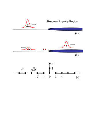
Figure 3: (Color online) Schematic illustration of the coherent separation process of a BT in the proposed optimal system. It consists of two semi-infinite uniform chains with different chemical potentials, resonant impurity. (a) An incident BT wavepacket comes from the left and scatters off the barrier. (b) The reflected waves contain the BT and the single particle wavepackets with different speeds. A single particle wavepacket moves along the resonant impurity region. (c) Schematic illustration of the equivalent effective Hamiltonian governs the evolution. For an optimal incident wavepacket, the success probability of the coherent separation approaches to unity.

The scheme to perform the coherent separation of a BT is based on the system depicted by the Hamiltonian

$$H_{\text{BTS}} = -t\left(\overset{0}{\sum_{i=-\infty}}+2\overset{\infty}{\sum_{i=2}}\right)a_{i}^{{\dagger}}a_{i+1}-\sqrt{2}ta_{1}^{{\dagger}}a_{2}+\text{H.c.}$$ (36)

$$+V\overset{\infty}{\sum_{i=-\infty}}n_{i}n_{i+1}+V\overset{\infty}{\sum_{i=2}}n_{i}.$$

To investigate the scattering process of an input BT wave from the left, one can establish an effective Hamiltonian in the quasi-invariant subspace spanned by the following basis $\{\underline{\left|l\right\rangle},l\in\left(-\infty,\infty\right)\}$ defined as

$$\underline{\left|l\right\rangle}\equiv\left\{\begin{array}[]{c}\text{Eqs. (\ref{Tri_basis}), }\left(l\leqslant 2\right)\\ a_{-1}^{{\dagger}}a_{0}^{{\dagger}}a_{l-1}^{{\dagger}}/\sqrt{2}\left|\text{vac}\right\rangle\text{, }\left(l>2\right)\end{array}\right..$$ (37)

The corresponding equivalent effective Hamiltonian can be written as

$$\mathcal{H}_{\text{BTS}} = -\sqrt{2}t\left(\sum_{l=-\infty}^{2}+\sqrt{2}\overset{+\infty}{\sum_{l=4}}\right)\underline{\left|l-1\right\rangle}\underline{\left\langle l\right|}-\sqrt{2}t\underline{\left|0\right\rangle}\underline{\left\langle 3\right|}$$ (38)

$$-\left(2-\sqrt{2}\right)t\overset{0}{\sum_{j=-\infty}}\underline{\left|3j+1\right\rangle}\underline{\left\langle 3j+2\right|}+\text{H.c.}$$

which is illustrated in Fig. 3 (c). The equivalent system is two connected semi-infinite chains with a side coupled two-site segment at the joint of them. In the optimal case, the perfect separation (or combination) process in the real space can be expressed as

$$\begin{split}&\left|\chi(+,-\infty)\right\rangle\left|\text{vac}\right\rangle\Longrightarrow\\ &r\left|\chi(-,-\infty)\right\rangle\left|\text{vac}\right\rangle+t\left|\varphi(+,+\infty)\right\rangle a_{-1}^{{\dagger}}a_{0}^{{\dagger}}\left|\text{vac}\right\rangle,\end{split}$$ (39)

and the corresponding inverse process as

$$\begin{split}&\left|\varphi(-,+\infty)\right\rangle a_{-1}^{{\dagger}}a_{0}^{{\dagger}}\left|\text{vac}\right\rangle\Longrightarrow\\ &r\left|\varphi(+,+\infty)\right\rangle a_{-1}^{{\dagger}}a_{0}^{{\dagger}}\left|\text{vac}\right\rangle+t\left|\chi(-,-\infty)\right\rangle\left|\text{vac}\right\rangle.\end{split}$$ (40)

This separation process is a little different from that of the BP. An incident three-particle wavepacket leaves two NN pair at the impurity, while a single-particle remains going forward. Numerical simulation is performed to evaluate the success probability of the previous scattering process. For an optimal Gaussian wavepacket with $\alpha=0.01$ the separation success probability is $0.97$ approximately.

VI Conclusion

In summary, we studied the BP and BT states in the extended Hubbard model. We found that, the resonant NN interaction can induce the BP and triple states. They are distinct from the known ones in the previous works, as their bandwidths are comparable to that of a single particle. In other words, the bandwidths of the bound clusters can be drastically widened by the NN interaction. We proposed relatively simple schemes to realize the coherent separation of these bound clusters. The exact result showed that the success probability of the coherent separation is unity for a BP while approached to unity for a BT in the optimal systems. We also studied the singlet BP in the extended Fermi-Hubbard system. We showed that the corresponding coherent separation process can be utilized to create long-distance entanglement without the need of temporal control and measurement process. Finally, we believe that our study will shed more light on the future research for multi-particle bound state.

We acknowledge the support of the CNSF (Grant Nos. 10874091 and 2006CB921205).

References

• (1) K. Winkler, G. Thalhammer, F. Lang, R. Grimm, J. H. Denschlag, A. J. Daley, A. Kantian, H. P. BΓΌchler and P. Zoller, Nature (London) 441, 853 (2006).
• (2) S. M. Mahajan and A. Thyagaraja, J. Phys. A 39, L667 (2006).
• (3) D. Petrosyan, B. Schmidt, J. R. Anglin, and M. Fleischhauer, Phys. Rev. A 76, 033606 (2007).
• (4) C. E. Creffield, Phys. Rev. A 75, 031607(R) (2007).
• (5) A. Kuklov and H. Moritz, Phys. Rev. A 75, 013616 (2007).
• (6) S. FΓΆlling, S. Trotzky, P. Cheinet, M. Feld, R. Saers, A. Widera, T. MΓΌller, and I. Bloch, Nature (London) 448, 1029 (2007).
• (7) S. ZΓΆllner, H.-D. Meyer, and P. Schmelcher, Phys. Rev. Lett. 100, 040401 (2008).
• (8) L. Wang, Y. Hao, and S. Chen, Eur. Phys. J. D 48, 229 (2008).
• (9) M. Valiente and D. Petrosyan, Europhys. Lett. 83, 30007 (2008); J. Phys. B 41, 161002 (2008).
• (10) L. Jin and Z. Song, Phys. Rev. A 79, 032108 (2009).
• (11) M. Valiente and D. Petrosyan, J. Phys. B 42, 121001 (2009).
• (12) M. Valiente, D. Petrosyan and A. Saenz, Phys. Rev. A 81, 011601(R) (2010).
• (13) S. Datta, Electronic Transport in Mesoscopic Systems (Cambridge University Press, Cambridge, 1995).
• (14) S. Yang, Z. Song and C. P. Sun, arXiv:0912.0324v1.
• (15) L. Jin and Z. Song, Phys. Rev. A 81, 022107 (2010).
• (16) W. Kim, L. Covaci, and F. Marsiglio, Phys. Rev. B 74, 205120 (2006).