Spin transfer in a ferromagnet-quantum dot and tunnel barrier coupled Aharonov-Bohm ring system with Rashba spin-orbit interactions

Abstract

The spin transfer effect in ferromagnet-quantum dot (insulator)-ferromagnet Aharonov-Bohm (AB) ring system with Rashba spin-orbit (SO) interactions is investigated by means of Keldysh nonequilibrium Green function method. It is found that both the magnitude and direction of the spin transfer torque (STT) acting on the right ferromagnet electrode can be effectively controlled by changing the magnetic flux threading the AB ring or the gate voltage on the quantum dot. The STT can be greatly augmented by matching a proper magnetic flux and an SO interaction at a cost of low electrical current. The STT, electrical current, and spin current are uncovered to oscillate with the magnetic flux. The present results are expected to be useful for information storage in nanospintronics.

I Introduction

The spin transfer effect (STE) states that when the spin-polarized electrons flow from one ferromagnet (FM) layer into another FM layer with magnetization aligned by a relative angle, they may transfer transverse spin angular momenta to the local spins of the second FM layer, thereby exerting a torque on the magnetic moments that is usually coined as the spin transfer torque (STT). This important phenomenon was predicted independently by Berger and Slonczeski J.C ; Berger in 1996 and soon confirmed by experiments. Because the STE can be utilized to switch the magnetic state of the free FM layer in a magnetic tunneling junction (MTJ) or a spin valve by applying an electrical current instead of a magnetic field, it may be even more useful in writing heads for magnetic random access memory (MRAM) or hard disk drivers than the conventional tunnel magnetoresistance (TMR) and giant magnetoresistance (GMR) effects. In view of the potentially wide applications in nanospintronic devices, a number of works on the STE have been done for different systems both theoretically and experimentally Zhu ; Mu1 ; Mu2 ; Ioannis ; Z.Z.Sun ; G.D ; Levy ; J.A ; Z.Li ; K.Xia ; G.D2 ; S.Zhang ; M.D ; K.Ando .

On the other hand, the quantum dot (QD) has received much attention in the past decades, and a lot of advances have been made in this particular field (e.g. Refs. I.Z ; Hanson ; J.Mar ; Xi ; Xi2 ). For a semiconductor QD, as the spin-orbit (SO) interaction is usually not negligible, some interesting phenomena related to the SO interactions, such as the bias-controllable intrinsic spin polarization in a QD Sun2 and the interplay of Fano and Rashba effect JPCM , can be observed. Almost twenty years ago, Datta and Das predicted a spin transistor based on the Rashba SO DD , showing that the SO interactions may be important in the semiconductor spintronics. However, the effect of the Rashba SO interaction on the STE is still sparsely studied. In this paper, we shall take the FM-QD (insulator, I)-FM Aharonov-Bohm (AB) ring system as an example to investigate how both the SO interaction and the magnetic flux affect the spin-dependent properties of the system by means of the nonequilibrium Green function method. We have found that the magnitude and direction of the STT can be easily controlled by changing the gate voltage $V_{g}$ on the QD or the magnetic flux $\phi$ through the ring if both the SO and electron-electron (e-e) interactions in the QD are considered, which might be useful in information storage.

The other parts of this paper are organized as follows. In Sec. II, a model is proposed, and the relevant Green functions are obtained in terms of the nonequilibrium Green function method. In Sec. III, the spin-dependent properties of STT in the system under interest are numerically investigated, and some discussions are presented. Finally, a brief summary is given in Sec. IV.

II MODEL AND METHOD

The system under interest is depicted in Fig. 1. Two FM leads spreading along the $z$ axis are weakly coupled to an insulating (I) barrier and a semiconducting QD, forming an AB ring. The left (L) FM electrode with the magnetization along the $z$ axis is applied by a bias voltage $-V/2$, while the right (R) electrode with the magnetization along the $z^{\prime}$ axis that deviates by an angle $\theta$ from the $z$ axis is applied by a bias voltage $V/2$. Assume that the QD is made of a two-dimensional electron gas in which the electrons are strongly confined in the $y$ direction by a potential $V(y)$. Due to $dV/dy\gg dV/dx$ and $dV/dz$, we have $\nabla V(\overrightarrow{y})\approx\widehat{y}(dV/dy)$, where $\widehat{y}$ is the unit vector along the $y$ axis. If $V(y)$ is asymmetric to $y=0$, both Rashba SO and e-e interactions on the QD should be considered. Since the electronic transport of the device along the $z$ axis is much more dominant than that along other two dimensions, the device under interest can be treated as a quasi one-dimensional system. Sun et al. Sun1  have carefully analyzed the SO Rashba interaction and found that (i) the Rashba SO interaction can be separated into two parts, $H_{R_{1}}$ and $H_{R_{2}}$, namely

$$H_{so} = \frac{\widehat{y}}{2\hbar}\cdot[\alpha(x)(\widehat{\sigma}\times\widehat{p})+(\widehat{\sigma}\times\widehat{p})\alpha(x)]=H_{R_{1}}+H_{R_{2}},$$ (1)

$$H_{R_{1}} = \frac{1}{2\hbar}[\alpha(x)\sigma_{z}p_{x}+\sigma_{z}p_{x}\alpha(x)],$$ (2)

$$H_{R_{2}} = -\frac{\alpha(x)\sigma_{x}p_{z}}{\hbar};$$ (3)

(ii) by choosing a suitable unitary transformation, $H_{R_{1}}$ can give rise to a spin-dependent phase factor in the tunneling matrix element between the leads and the QD, while Eq. (3) can be written in the second-quantization form as Sun1 : $H_{R_{2}}=\sum\limits_{mn}(t_{mn}^{so}d_{m\downarrow}^{+}d_{n\uparrow}+h.c.)$, that causes a spin-flip term with strength $t_{mn}^{so}$ in the QD, where $m$ and $n$ are quantum numbers for the eigenstates of electrons in QD; (iii) since the time-reversal invariance is maintained by the Rashba SO interaction, $t_{mn}^{so}=-t_{nm}^{so}$ and $t_{nn}^{so}=0$, which suggests that the spin-flip scatterings only occur between different levels in the QD. In the present work, for simplicity, we shall consider the case with a single-level QD as in some previous works Sun1 ; JPCM , where no interlevel spin-flip scattering happens in the QD. Thus, $H_{R_{2}}$ equals to zero. Suppose that $\alpha(x)$ is independent of the coordinates in the scattering region, and a magnetic flux penetrates into the AB ring. The Hamiltonian of the present system is given by

$$H=H_{QD}+H_{\beta}+H_{T},$$ (4)

$$H_{QD}=\sum\limits_{\sigma}\varepsilon_{d}d_{\sigma}^{+}d_{\sigma}+Un_{\uparrow}n_{\downarrow},$$ (5)

$$H_{\beta}=\sum\limits_{\beta k,\sigma}\varepsilon_{\beta k\sigma}a_{\beta k\sigma}^{+}a_{\beta k\sigma},$$ (6)

$$H_{T} = \sum\limits_{k,\sigma}[t_{Rd}(\cos\frac{\theta_{\beta}}{2}a_{Rk\sigma}^{+}-\sigma\sin\frac{\theta_{\beta}}{2}a_{Rk\overline{\sigma}}^{+})\times e^{-i\sigma\gamma}e^{i\phi}d_{\sigma}+h.c.]$$ (7)

$$+\sum\limits_{k,\sigma}[t_{Ld}a_{Lk\sigma}^{+}d_{\sigma}+h.c.]$$

$$+\sum\limits_{k,\sigma}[t_{LR}(\cos\frac{\theta_{\beta}}{2}a_{Rk\sigma}^{+}-\sigma\sin\frac{\theta_{\beta}}{2}a_{Rk\overline{\sigma}}^{+})a_{Lk\sigma}+h.c.],$$

where $a_{\beta k\sigma}$ and $d_{\sigma}$ are annihilation operators of electrons with momentum $k$ and spin $\sigma$ $(=\uparrow,\downarrow)$ in the $\beta$ $(=L,R)$ electrode and in the QD, respectively, $\varepsilon_{\beta k\sigma}=\varepsilon_{k}+\sigma{}M_{\beta}-eV_{\beta}$ is the single-electron energy for the wave vector $k$ with the molecular field $M_{\beta}$ in the electrode $\beta$, $\varepsilon_{d}$ is the single-electron energy in the QD, $U$ represents the on-site Coulomb interaction between electrons in the QD, $t_{\beta d}$ is the tunneling matrix element of electrons between the $\beta$ electrode and the QD, $t_{LR}$ is the tunneling matrix element of electrons between $L$ and $R$ electrodes through the insulating barrier, $n_{\sigma}=c_{\sigma}^{+}c_{\sigma}$, and $\gamma=$ $k_{R}d$ with $k_{R}\equiv\alpha m^{\ast}/\hbar^{2}$, $\alpha=\langle\Psi(y)\left|(d/dy)V(y)\right|\Psi(y)\rangle$, $m^{\ast}$ the effective mass of electrons and $d$ the thickness of the middle region. The magnetic flux $\Phi$ threading the AB ring is related to the phase factor by $\phi=2\pi\Phi/\Phi_{0}$, where $\Phi_{0}$ is the flux quantum. It should be noted that the magnetic flux threading the AB ring generally includes two contributions, one generated by the FM leads that may be small and constant, and the other from the external magnetic field that can be varied to adjust the phase factor $\phi$.

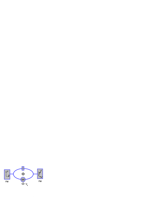
Figure 1: A schematic layout of FM-QD(I)-FM AB ring system. The electrons flow towards the $x$ axis.

The transverse component of the total spin in the right FM lead can be written as Zhu

$$S = \frac{\hbar}{2}\sum\limits_{k}\left(a_{Rk\uparrow}^{+},a_{Rk\downarrow}^{+}\right)\hat{\sigma}_{x}\left(\begin{array}[]{c}a_{Rk\uparrow}\\ a_{Rk\downarrow}\end{array}\right)$$ (10)

$$= \frac{\hbar}{2}\sum\limits_{k}(a_{Rk\uparrow}^{+}a_{Rk\downarrow}+a_{Rk\downarrow}^{+}a_{Rk\uparrow}),$$ (11)

where $S$ is written in the $x^{\prime}y^{\prime}z^{\prime}$ coordinate frame. The spin torque, namely, the time evolution rate of the transverse component of the total spin of the right FM lead, can be obtained by $\partial S/\partial t=\frac{i}{\hbar}\langle[H,S]\rangle$. According to Refs. X.W1 ; X.W2 ; Zhu , the right FM layer gains two types of torques: one is the equilibrium torque caused by the spin-dependent potential, and another is from the tunneling of electrons that is in what we are interested. After cautiously separating the current-induced torque from the equilibrium one, the STT is given by

$$\tau = -\Re e\{t_{Rd}e^{i\gamma}e^{i\phi}\cos\frac{\theta}{2}G_{d\downarrow R\uparrow}^{<}(t,t)-t_{Rd}e^{-i\gamma}e^{i\phi}\sin\frac{\theta}{2}G_{d\uparrow R\uparrow}^{<}(t,t)$$ (12)

$$+t_{RL}\cos\frac{\theta}{2}G_{L\downarrow R\uparrow}^{<}(t,t)-t_{RL}\sin\frac{\theta}{2}G_{L\uparrow R\uparrow}^{<}(t,t)$$

$$+t_{Rd}e^{-i\gamma}e^{i\phi}\cos\frac{\theta}{2}G_{d\uparrow R\downarrow}^{<}(t,t)+t_{Rd}e^{i\gamma}e^{i\phi}\sin\frac{\theta}{2}G_{d\downarrow R\downarrow}^{<}(t,t)$$

$$+t_{RL}\cos\frac{\theta}{2}G_{L\uparrow R\downarrow}^{<}(t,t)+t_{RL}\sin\frac{\theta}{2}G_{L\downarrow R\downarrow}^{<}(t,t)\}.$$

From Eq. (9), it is clear that the current-induced STT can be obtained as long as we get the lesser Green functions $G^{<}$. In what follows we shall use Keldysh’s nonequilibrium Green function technique to determine all lesser Green functions Jauho . These functions are closely related to the retarded Green functions defined by

$$G_{\beta\sigma\gamma\sigma^{\prime}}^{r}(t,t^{\prime}) = -i\theta(t-t^{\prime})\langle\{\sum\limits_{k^{{}^{\prime}}}a_{\beta k^{{}^{\prime}}\sigma}(t),\sum\limits_{k}a_{\gamma k\sigma^{\prime}}^{+}(t^{\prime})\}\rangle,$$

$$G_{\beta\sigma d\sigma^{\prime}}^{r}(t,t^{\prime}) = -i\theta(t-t^{\prime})\langle\{\sum\limits_{k}a_{\beta k\sigma}(t),d_{\sigma^{\prime}}^{+}(t^{\prime})\}\rangle,$$

$$G_{d\sigma d\sigma^{{}^{\prime}}}^{r}(t,t^{\prime}) = -i\theta(t-t^{\prime})\langle\{d_{\sigma}(t),d_{\sigma^{\prime}}^{+}(t^{\prime})\}\rangle,$$

where $\{A,B\}$ denotes the anticommutation relations, and $\langle A\rangle$ stands for the thermal average. By using the equation of motion, the retarded Green functions can be obtained by Dyson equation $G^{r}=g^{r}+g^{r}\Sigma^{r}G^{r}$, where $g^{r}$ is the retarded Green function for decoupled systems, and $\Sigma^{r}$ is the self-energy of electrons. To obtain $G^{r}$, the decoupling approximations similar to those in Refs. Mu2 ; Xi3 ; Jauho for the equations of motion of Green functions should be made. As the associated equations for Green functions are quite lengthy, we shall not repeat them here for conciseness.

The lesser Green function $G^{<}$ can be calculated straightforwardly from the Keldysh equation

$$G^{<} = (1+G^{r}\Sigma^{r})g^{<}(1+\Sigma^{a}G^{a})+G^{r}\Sigma^{<}G^{a}$$ (13)

$$= G^{r}g^{r-1}g^{<}g^{a-1}G^{a}+G^{r}\Sigma^{<}G^{a}.$$

In the present case, $\Sigma^{<}=0$, and $g^{r-1}g^{<}g^{a-1}$ is diagonal

$$g^{r-1}g^{<}g^{a-1}=\left(\begin{array}[]{cccccc}2if_{L}(\varepsilon)/\pi\rho_{L\uparrow}&&&&&\\ &2if_{L}(\varepsilon)/\pi\rho_{L\downarrow}&&&&\\ &&2if_{R}(\varepsilon)/\pi\rho_{R\uparrow}&&&\\ &&&2if_{R}(\varepsilon)/\pi\rho_{R\downarrow}&&\\ &&&&0&\\ &&&&&0\end{array}\right).$$ (14)

The electrical current is given by

$$I = I_{\uparrow}+I_{\downarrow},$$ (15)

$$I_{\uparrow} = -\Re e\{t_{Rd}e^{-i\gamma}e^{i\phi}\cos\frac{\theta}{2}G_{d\uparrow R\uparrow}^{<}(t,t)+t_{Rd}e^{i\gamma}e^{i\phi}\sin\frac{\theta}{2}G_{d\downarrow R\uparrow}^{<}(t,t)$$ (16)

$$+t_{RL}\cos\frac{\theta}{2}G_{L\uparrow R\uparrow}^{<}(t,t)+t_{RL}\sin\frac{\theta}{2}G_{L\downarrow R\uparrow}^{<}(t,t)\},$$

$$I_{\downarrow} = -\Re e\{t_{Rd}e^{i\gamma}e^{i\phi}\cos\frac{\theta}{2}G_{d\downarrow R\downarrow}^{<}(t,t)-t_{Rd}e^{-i\gamma}e^{i\phi}\sin\frac{\theta}{2}G_{d\uparrow R\downarrow}^{<}(t,t)$$ (17)

$$+t_{RL}\cos\frac{\theta}{2}G_{L\downarrow R\downarrow}^{<}(t,t)-t_{RL}\sin\frac{\theta}{2}G_{L\uparrow R\downarrow}^{<}(t,t)\}.$$

The spin current is defined by a difference between the electrical currents of spin up and down,

$$I_{s}=I_{\uparrow}-I_{\downarrow}.$$ (18)

To get the physical quantities of interest, the above-mentioned equations will be solved numerically in a self-consistent manner.

III RESULTS AND DISCUSSIONS

It has been shown that when the incident electrical current is larger than a critical value, the STT can switch the direction of the magnetization of the free FM layer clockwise or anticlockwise depending on the direction of the incident electrical current J.Z ; J.Z.Sun ; Xi3 . In the present case, the positive STT tends to push the spins in the right FM electrode aligning antiparallel with the magnetization of the left FM electrode, while the negative STT may cause a reverse orientation of the magnetization in the free FM layer. In order to properly incorporate the STE into a functionalized spintronic device, both the direction and magnitude of the STT should be taken into account. For simplicity, in the following parts we will assume that in most cases the left and right FM electrodes have the same spin polarization $P_{L}=P_{R}=P=0.5$, and the angle $\theta$ between $z$ and $z^{\prime}$ axes is $\pi/3$ throughout the paper unless specified. We take $I_{0}=\frac{e\Gamma_{0}}{\hbar}$ and $\Gamma_{0}=\Gamma_{L(R)\uparrow}(P=0)=\Gamma_{L(R)\downarrow}(P=0)$ as scales for the electrical and spin currents as well as the STT and energy, respectively, where $\Gamma_{\alpha\sigma}(\varepsilon)=2\pi\sum\nolimits_{k_{\alpha}}\left|t_{\alpha d}\right|^{2}\delta(\varepsilon-\varepsilon_{k_{\alpha}})$. In accordance with Refs. F.M ; T.M ; D.G , we assume that the Rashba SO interaction constant is $\alpha\sim 3\times 10^{-11}eVm$, $k_{R}=m^{\ast}\alpha/\hbar^{2}\approx 0.015/nm$ for $m^{\ast}=0.036m_{e}$, the typical length of QD is $100$ $nm$, $U=5\Gamma_{0}$, and $\gamma$ can be $\pi/2$ or larger.

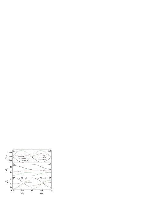
Figure 2: (Color Online) The $\theta$ dependence of (a) the spin transfer torque $\tau$, (b) the electrical current $I$, and (c) the spin current $I_{s}$ for different magnetic flux $\phi$. The $\theta$ dependence of (d) the spin transfer torque $\tau$, (e) the electrical current $I$, and (f) the spin current $I_{s}$ for different Rashba SO interaction $\gamma$.

As the STE only exists in the noncollinear case, in contrast to previous works where the electrical and spin currents were discussed only in collinear cases ($\theta=0$ or $\pi$) (e.g. Sun1 ; JPCM ), let us first look at the angular dependences of the STT, the electrical current and spin current for different magnetic flux $\phi$ and Rashba SO interaction $\gamma$. The results are given in Fig. 2, where $\gamma=\pi/2$ and $\varepsilon_{d}=1$ in Figs. 2(a)-(c), and $\phi=\pi/2$ and $\varepsilon_{d}=1$ in Figs. 2(d)-(f). It can be observed that the STT has a sine-like relationship with the relative angle $\theta$, and the direction and magnitude of the STT are clearly influenced by both the magnetic flux $\phi$ and Rashba SO interaction $\gamma$. In the absence of either $\phi$ or $\gamma$, the STT remains negative (anticlockwise). For the simultaneous presence of $\phi$ and $\gamma$ (greater than $\pi/4$), the STT becomes positive (clockwise). This fact reminds us that we may apply the magnetic flux to change the direction of the STT, thereby being capable of manipulating the magnetic state of the free FM layer, which might be useful for information storage and for designing the memory element. The electrical current $I$ decreases with increasing $\theta$ in the absence of either $\phi$ or $\gamma$, indicating a spin-valve effect, while it increases with $\theta$ in the presence of both $\phi$ and $\gamma$ (greater than $\pi/4$), giving an anti-spin-valve effect [e.g. $\phi$ or $\gamma=\pi/2$ in Figs. 2(b) and (e)]. This property differs obviously from the conventional FM-I-FM or FM-QD-FM systems without considering the SO interactions where the electrical current always decreases with increasing $\theta$. The spin current shows a feature similar to the electrical current. From these calculated results presented in Fig. 2, we can find that for a given Rashba SO interaction $\gamma$ (magnetic flux $\phi$), the angular dependent STT, electrical current and spin current exhibit distinct behaviors for different magnetic flux (Rashba SO interaction).

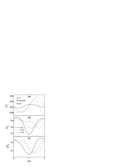
Figure 3: (Color Online) The magnetic flux dependence of (a) spin transfer torque $\tau$, (b) electrical current $I$, and (c) spin current $I_{s}$ for different Rashba SO interaction $\gamma$, where $\varepsilon_{d}=-1$, and $\theta=\pi/3$.

Figure 3 shows the magnetic flux $\phi$ dependence of the STT, electrical current and spin current for different Rashba SO interactions. We can see that with increasing $\phi$, the STT, electrical current and spin current oscillate differently for various Rashba SO interactions $\gamma$. The larger the SO interaction $\gamma$ is, the more complex the oscillations are. For the QD energy level $\varepsilon_{d}=-1$ and $\gamma=\pi/2$, the STT shows a maximum around $\phi=3\pi/2$, while the electrical current exhibits minima around the same $\phi$. Therefore, we may be able to use a lower current to change the magnetic state of the free FM by adjusting the magnetic flux penetrating into the AB ring. It is favorable for the spintronic devices, because a larger current may cause more heating, while the heating should be reduced as small as possible for better functions of the device. In addition, it can be found that the STT is closely related to the spin current, as the dips and peaks of Figs. 3(a) and (c) appear almost at the same positions.

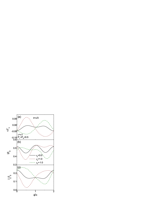
Figure 4: (Color Online) The magnetic flux dependence of (a) the spin transfer torque $\tau$, (b) the electrical current $I$, and (c) the spin current $I_{s}$ for different energy levels $\varepsilon_{d}$, where $\theta=\pi/3$, and $\gamma=\pi/2$.

The energy level $\varepsilon_{d}$ of electrons in the QD, that offers resonant tunneling channels for spin-polarized electrons from the left FM electrode to the right FM one, has also effects on the magnetic flux $\phi$ dependence of the STT, electrical current and spin current. The results are presented in Fig. 4 for $\gamma=\pi/2$. It is unclosed that for different $\varepsilon_{d}$, $\tau$, $I$ and $I_{s}$ exhibit different features, and oscillate with $\phi$ in general. When $\varepsilon_{d}=0,$ $\tau$, $I$, and $I_{s}$ are mirror symmetrical to $\phi=\pi$, and $\tau$ is always negative. For positive and negative $\varepsilon_{d}$, $\tau$ and $I_{s}$ have just opposite properties: the peaks at $\phi=\pi/2$ (dips at $\phi=3\pi/2$) for $\varepsilon_{d}=1$ correspond to the dips (peaks) for $\varepsilon_{d}=-1$ at the same $\phi$, but the curves for positive and negative $\varepsilon_{d}$ intersect at $\phi=\pi$, as shown in Figs. 4(a) and (c). It hints us that by changing the gate voltage that is usually utilized to alter the energy levels $\varepsilon_{d}$ in the QD, one can adjust the STT. For example, when $\phi=\pi/2$, if we change $\varepsilon_{d}$ from $-1$ to $1$, the STT changes from $0.06$ anticlockwise to $0.075$ clockwise. As the gate voltage is easier than the magnetic flux to control, the present observation may offer a useful way to manipulate the magnetic state of the free FM layer. The electrical current also displays quite different oscillating behaviors for $\varepsilon_{d}=1$ and $-1$, which is shown in Fig. 4(b).

Why can the STT be controlled by changing the magnetic flux and gate voltage? Because the transmission probability of the spin-up electrons is proportional to $cos(\theta+\phi+\gamma)$ and that of spin-down electrons is proportional to $cos(\theta+\phi-\gamma)$ Sun1 . The spin-up and spin-down electrons have different transmission probabilities if $\gamma$ is nonzero, leading to oscillations of the STT with magnetic flux $\phi$. On the other hand, the STT is intimately related to the electrical current $I$ Mu2 , and the magnitude of $I$ depends on the energy level $\varepsilon_{d}$ of QD, so it is reasonable that the STT can be manipulated by adjusting the gate voltage. $I_{\uparrow}$ and $I_{\downarrow}$ give rise to opposite STT on the right FM layer. Since $I_{\uparrow}$ and $I_{\downarrow}$ oscillate for various combination of $\phi$ and $\gamma$ in different ways, the STT may reach the maximum while $I$ is in its minimum when $\phi$ and $\gamma$ take proper values.

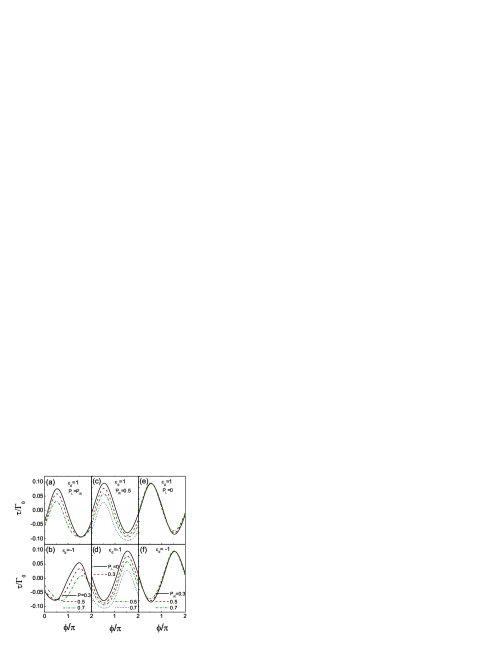
Figure 5: (Color Online) The magnetic flux dependence of the spin transfer torque for different spin polarizations at $\theta=\pi/3$, and $\gamma=\pi/2$.

In addition, the spin polarization $P_{L,R}$ of the FM electrodes has also effects on the magnetic flux dependence of the STT, as shown in Fig. 5. Generally, with increasing $P_{L,R}$, the STT shows qualitatively similar behaviors for positive and negative $\varepsilon_{d}$. When $P_{L}=P_{R}=P$, as shown in Figs. 5(a) and (b), the larger the polarization $P$, the smaller the peaks of the STT. For different $P$, $\tau$ has obvious changes when $0<\phi<3\pi/2$ for $\varepsilon_{d}=1$, and when $\pi/2<\phi<\pi$ for $\varepsilon_{d}=-1$. When $P_{R}$ and $P_{L}$ are different, e.g. $P_{R}=0.5$ and $P_{L}=0$, $0.3$, $0.7$, the larger $P_{L}$ is, the more downward the curves move, as indicated in Figs. 5(c) and (d). It is interesting that even the left electrode becomes spin unpolarized ($P_{L}=0$), the STT as a function of $\phi$ still behaves a sine-like curve and retains almost intact for different spin polarizations $P_{R}$ [Figs. 5(e) and (f)]. The existence of the STT at $P_{L}=0$ demonstrates that even if the left electrode is a normal metal (NM), the unpolarized electrons from the left NM lead flowing into the AB ring system with an QD encompassed by a magnetic flux $\phi$ can become spin-polarized before entering into the right FM electrode. It is apprehensible , because owing to the Rashba effect, the spin-up and spin-down electrons pass through the AB ring system at different transmission probabilities, as discussed above. When these spin-polarized electrons flow into the right FM layer, they may transfer some spin angular momenta to the local spins of the right FM electrode, thereby giving rise to the STT. In this case, if $\phi=0$, the STT becomes negligibly small. In the above analysis, we have presumed that the spin relaxation time of electrons is greater than that of the tunneling time. Thus, to ensure the feasibility of experimental observation, one must choose proper materials as FM electrodes and QD, and design a viable ring system to meet with the above requirements. It is interesting to note that a similar mesoscopic ring system was proposed, where some material parameters were discussed for possible experimental implementation radu that may be insightful for choosing proper materials for designing the present ring system.

The effect of Rashba SO interaction $\gamma$ on the STT, electrical current and spin current is shown in Fig. 6 for different magnetic flux $\phi$. With increasing $\gamma$, when $\phi=0,$ the STT is always negative and goes down non-monotonously. When $\phi=\pi/4$ or $\pi/2$, $\tau$ goes up from negative to positive, reaches a round maximum, and then decreases, as depicted in Figs. 6(a). This result implies that the STT can be enhanced remarkably by matching $\phi$ with proper $\gamma$. The $\gamma$ dependences of the electrical current and spin current show different behaviors for various $\phi$, as presented in Figs. 6(b) and (c). With increasing $\gamma$, for $\phi=0$, both $I$ and $I_{s}$ increase; for $\phi=\pi/4$, $I$ first decreases to a round minimum, and then goes up, while $I_{s}$ declines slowly; for $\phi=\pi/2$, the situation becomes reverse, i.e., $I$ decreases dramatically, while $I_{s}$ first declines and then goes up. In a word, the Rashba SO interactions have various effects on the STT, electrical current and spin current.

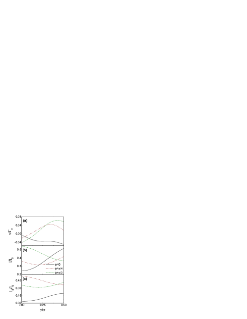
Figure 6: (Color Online) The Rashba SO interaction $\gamma$ dependence of (a) the spin transfer torque $\tau$, (b) the electrical current $I$, and (c) the spin current $I_{s}$ for different magnetic flux $\phi$, where $\theta=\pi/3$, and $\varepsilon_{d}=1$.

Finally, the bias voltage dependences of the STT, electrical current and spin current are studied for different $\gamma$ and $\phi$, as shown in Fig. 7. In the simultaneous presence of $\gamma$ and $\phi$, e.g. $\gamma=\phi=\pi/2$, with increasing the voltage, the STT first increases almost linearly, reaches a peak, and then decreases slowly. After reaching zero, it starts to increase again in a different direction. In the absence of either $\gamma$ or $\phi$ or both, $\tau$ is negative, and decreases non-monotonously with increasing the bias voltage, as indicated in Fig. 7(a). For various combinations of $\gamma$ and $\phi$, the electrical current $I$ exhibits qualitatively similar behaviors, which increases overall in a non-ohmic way with increasing the bias [Fig. 7(b)]. For $\gamma=\phi$, $I_{s}$ remains almost constant at a small bias. When the bias passes a threshold, it increases linearly with the increase of $V$. For $\gamma\neq\phi$, $I_{s}$ grows up almost linearly despite of small shoulders at a low bias, as displayed in Fig. 7(c). From Figs. 7(a) and (c), we can see that the shoulder structure of the STT and the threshold of the spin current appear around $eV=2\varepsilon_{d}$, where the resonant tunneling happens. It is not surprising that the resonant tunneling has influences on the spin-dependent transport of the system. However, it is more important when $\gamma=\phi$, while it is negligible when $\gamma\neq\phi$.

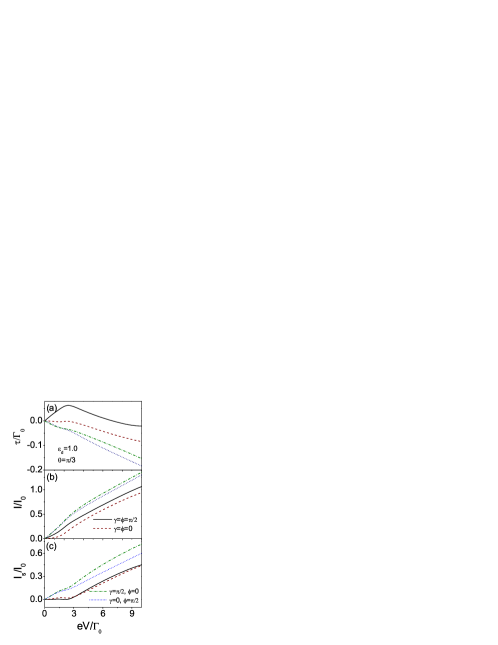
Figure 7: (Color Online) The bias voltage dependence of (a) the spin transfer torque $\tau$, (b) the electrical current $I$, and (c) the spin current $I_{s}$ for different $\gamma$ and $\phi$.

IV Summary

By means of the Keldysh nonequilibrium Green function method, we have investigated the STE in the FM-QD(I)-FM ring system with Rashba SO interactions. It has been found that both the direction and magnitude of the STT are affected by the magnetic flux and the Rashba SO interactions. When the SO interaction is strong enough, the STT acting on the spins of the right FM electrode can be remarkably enhanced by matching the magnetic flux through the AB ring, which makes it is possible to readily manipulate the magnetic state of the free FM layer at a cost of lower electrical current. This property is quite expected for nanospintronic devices where the excessive heating generated by the electrical current should be avoided as much as possible. It has also been uncovered that by adjusting the gate voltage acting on the QD, both the magnitude and the direction the STT can be changed, which gives an alternative way to manipulate the magnetic state of the free FM layer. In addition, it is interesting to observe that the STT can also be increased by the magnetic flux through the ring or the gate voltage on the QD even if the left FM lead is changed to a NM.

We would like to mention that the results presented in this paper provide useful information for designing practical spintronic devices based on the STE. Such a ring layout can be used either as a memory element with a low driving current or as a magnetometer to measure weak magnetic fields, because the tunnel current depends sensitively on the magnetic flux threaded the ring. On the other hand, the tunnel current or the magnetic state of the free FM layer are affected by the Rashba SO interaction, and one may inversely enable to estimate the magnitude of the Rashba SO interaction on the QD by means of such a ring apparatus. We expect that the present theoretical findings could be tested experimentally in future.

- (1) Berger L 1996 Phys. Rev. B 54 9353
- (2) Slonczewski J C 1996 J. Magn. Magn. Mater. 159 L1
- (3) Zhu Z G, Su G, Zheng Q R, and Jin B 2003 Phys. Rev. B 68 224413; 2003 Phys. Lett. A 306 249
- (4) Mu H F, Zheng Q R, Jin B, and Su G 2005 Phys. Lett. A 336 66
- (5) Mu H F, Su G and Zheng Q R 2006 Phys. Rev. B 73 054414
- (6) Theodonis I, Kioussis N, Kalitsov A, Chshiev M and Butler W H 2006 Phys. Rev. Lett 97 237205
- (7) Sun Z Z and Wang X R 2006 Phys. Rev. Lett 97 077205
- (8) Fuchs G D, Katine J A, Kiselev S I, Mauri D, Wooley K S, Ralph D C and Buhrman R A 2006 Phys. Rev. Lett 96 186603
- (9) Levy P M and Fert A, Phys. Rev. Lett 2006 97 097205
- (10) Katine J A, Albert F J, and Buhrman R A 2000 Phys. Rev. Lett 84 3149
- (11) Li Z and Zhang S 2004 Phys. Rev. Lett 92 207203
- (12) Xia K, Kelly P J, Bauer G E W, Brataas A, and Turek I 2002 Phys. Rev. B 65 220401(R)
- (13) Fuchs G D, Krivorotov I N, Braganca P M, Emley N C, Garcia A G F, Ralph D C, and Buhrman R A 2005 Appl. Phys. Lett 86 152509
- (14) Zhang S, Levy P M, and Fert A 2000 Phys. Rev. Lett 88 236601
- (15) Stiles M D and Zangwill A 2002 Phys. Rev. B 66 014407
- (16) Ando K, Takahashi S, Harii K, Sasage K, Ieda J, Maekawa S, and Saitoh E 2008 Phys. Rev. Lett 101 036601
- (17) Zutic I, Fabian J, and Sarma S D 2004 Rev. Mod. Phys 76 323
- (18) Harson R, Kouhenhoven L P, Petta J R, Tarucha S and Vandersypen L M K 2007 79 1271
- (19) Martinek J, Utsumi Y, Imamura H, Barnaś J, Maekawa S, König J, and Schön G 2003 Phys. Rev. Lett 91 127203
- (20) Chen X, Zheng Q R, and Su G 2007 Phys. Rev. B 76 144409
- (21) Chen X, Mu H F, Zheng Q R and Su G 2006 Phys. Lett. A 358 47
- (22) Sun Q F, Xie X C 2006 Phys. Rev. B 73 235301
- (23) Ying Y, Jin G and Ma Y 2009 J. Phys.: Condens. Matter 21 275801
- (24) Datta S and Das B 1990 Appl. Phys. Lett 56 665
- (25) Sun Q F, Wang J and Guo H 2005 Phys. Rev. B 71 165310
- (26) Waintal X and Brouwer P W 2001 Phys. Rev. B 63 220407
- (27) Waintal X and Brouwer P W 2002 Phys. Rev. B 65 054407
- (28) Haug H and Jauho A P Quantum Kinetics in Transport and Optics of Semiconductors (Springer, Berlin, 1998), p.166
- (29) Sun J Z 2000 IBM J. Res. & Dev. 50 81
- (30) Sun J Z 2000 Phys. Rev. B 62 570
- (31) Chen X, Zheng Q R, and Su G 2008 Phys. Rev. B 78, 104410
- (32) Mireles F and Kirzenow G 2001 Phys. Rev. B 68 115316
- (33) Matsuyama T, Kursten R, Meissner C and Merkf U 2000 Phys. Rev. B 61 15588
- (34) Grundler D 2000 Phys. Rev. Lett 84 6074
- (35) Ionicioiu R and D’Amico I 2003 Phys. Rev. B 67 041307(R)