On the suspected timing error in Wilkinson microwave anisotropy probe map-making

Abstract

Context. It has recently been suggested that the compilation of the calibrated time-ordered-data (TOD) of the Wilkinson Microwave Anisotropy Probe (WMAP) observations of the cosmic microwave background (CMB) into full-year or multi-year maps may have been carried out with a small timing interpolation error. A large fraction of the previously estimated WMAP CMB quadrupole signal would be an artefact of incorrect Doppler dipole subtraction if this hypothesis were correct.

Aims. Since observations of bright foreground objects constitute part of the TOD, these can be used to test the hypothesis.

Methods. Scans of an object in different directions should be shifted by the would-be timing error, causing a blurring effect. For each of several different timing offsets, three half-years of the calibrated, filtered WMAP TOD are compiled individually for the four W band differencing assemblies (DA’s), with no masking of bright objects, giving 12 maps for each timing offset. Percentiles of the temperature-fluctuation distribution in each map at HEALPix resolution $N_{\mathrm{side}}=2048$ are used to determine the dependence of all-sky image sharpness on the timing offset. The Q and V bands are also considered.

Results. In the W band, which is the band with the shortest exposure times, the 99.999% percentile, i.e. the temperature fluctuation in the $\approx$ 503-rd brightest pixel, is the least noisy percentile as a function of timing offset. Using this statistic, the hypothesis that a $-25.6$ ms offset relative to the timing adopted by the WMAP collaboration gives a focus at least as sharp as the uncorrected timing is rejected at $4.6\sigma$ significance, assuming Gaussian errors and statistical independence between the maps of the 12 DA/observing period combinations. The Q and V band maps also reject the $-25.6$ ms offset hypothesis at high statistical significance.

Conclusions. The requirement that the correct choice of timing offset must maximise image sharpness implies that the hypothesis of a timing error in the WMAP collaboration’s compilation of the WMAP calibrated, filtered TOD is rejected at high statistical significance in each of the Q, V and W wavebands. However, the hypothesis that a timing error was applied during calibration of the raw TOD, leading to a dipole-induced difference signal, is not excluded by this method.

1 Introduction

The nature of the large-scale cosmic microwave background (CMB) signal in the Wilkinson Microwave Anisotropy Probe (WMAP) observations (Bennett et al. 2003b) is of fundamental importance to observational cosmology. A lack of structure on the largest scales in maps of CMB temperature fluctuations would be a hint that the comoving spatial section of the Universe is multiply connected (de Sitter 1917; Friedmann 1923, 1924; Lemaître 1931; Robertson 1935) and that its size may have been detected (Starobinsky 1993; Stevens et al. 1993). The WMAP observations have confirmed that the large-scale CMB signal analysed either as a quadrupole signal or as a two-point autocorrelation function signal is weak (Spergel et al. 2003; Copi et al. 2007, 2009). Several analyses indicate that either a $T^{3}$ comoving space (Spergel et al. 2003; Aurich et al. 2007; Aurich 2008; Aurich et al. 2008, 2010) or a Poincaré dodecahedral space ($S^{3}/I^{*}$) model (Luminet et al. 2003; Aurich et al. 2005a, 2005b; Gundermann 2005; Caillerie et al. 2007; Roukema et al. 2008a, 2008b) fit the WMAP data better than an infinite, simply connected flat model, while other analyses disagree (Key et al. 2007; Niarchou & Jaffe 2007). Highly significant evidence for either an infinite or a finite model of comoving space has not yet been obtained.

Liu & Li (Liu & Li 2008; Li et al. 2009; Liu & Li 2009; Liu et al. 2010) have suggested that several systematic errors may have been made in the data analysis pipelines used by the WMAP collaboration in the compilation of their original time-ordered-data (TOD) into single-year or multi-year maps. Liu & Li (2008) recommended that new maps should be made using the full TOD in order to avoid some of these suspected errors. This requires moderately heavy computational resources (RAM and CPU) on typical present-day desktop computers. Aurich et al. (2010) sidestepped this by using a phenomenological correction for the hot pixel effect (Liu & Li 2008). They found that their correction applied to the 5-year WMAP W band data removes the anti-correlation in temperature fluctuations at angular separations of nearly 180^∘ and improves the fit of a $T^{3}$ model to the data.

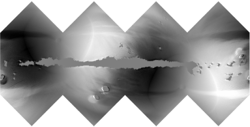
Figure 1: Dipole-induced difference all-sky map using the WMAP quaternion history of the first year of WMAP observations and $\delta t=0$ in the V band, i.e. a timing offset of $-38.4$ ms (see Sect. 2.2), shown in the hybrid, cylindrical equal-area (Lambert 1772), interrupted Collignon (Collignon 1865) spherical projection, i.e. the HEALPix ($H=4,K=3$) spherical projection (Roukema & Lew 2004; Calabretta & Roukema 2007; Górski et al. 2005), centred on the Galactic Centre, with latitude increasing upwards and longitude increasing to the left. The grey scale is linear from $-10\mu$K (black) to $+10\mu$K (white). No sky observations are used, i.e. only Liu et al. (2010)’s Eqs (1) and (2) as encoded in their software are used to process the quaternion data. Standard sky masks are used. This is the 80-th map iteration.

Liu & Li (2009) carried out a full analysis of the 5-year WMAP TOD. Their analysis pipeline appeared to give test results largely compatible with those of the WMAP collaboration. However, the CMB quadrupole amplitude was found to be much weaker, and sub-degree power was also found to be a little weaker. Later, Liu et al. (2010) traced the difference between their analysis and that of the WMAP collaboration to a difference in interpolating the timing of individual observations from the times recorded in the TOD files. The TOD FITS format files contain observational starting times in both the “Meta Data Table” and the “Science Data Table”. The full set of observing times of individual observations are not recorded in either data table; they must be interpolated from the smaller set of observing times that are recorded. The starting times in the Meta Data Table are 25.6 ms greater than the corresponding times in the Science Data Table. A computer script for checking this is given in Appendix A. The durations of individual observations in the Q, V and W bands are 102.4 ms, 76.8 ms, and 51.2 ms, respectively (Section 3.2, Limon et al. 2010). The 21 April 2010 version of the WMAP Explanatory Supplement (Section 3.1, Limon et al. 2010) discusses the relation between the start times in the two tables, but does not refer to the 25.6 ms offset, i.e. half of a W band observing interval or a quarter of a Q band observing interval. Bennett et al. (2003a) state (Sect. 6.1.2) that “a relative accuracy of 1.7 ms can be achieved between the star tracker(s), gyro and the instrument”, i.e. the combined random and systematic error should be much smaller than 25.6 ms. Given that the timing offset is numerically implicit in the WMAP TOD files, it could, strictly speaking, be referred to as the WMAP collaboration’s “implicitly claimed but ignored” timing offset. However, for simplicity, the timing offset will be referred to here as Liu et al. (2010)’s hypothesis.

Using their Eqs (1) and (2), Liu et al. (2010) showed that the error in estimating the Doppler dipole of the spacecraft velocity implied by the would-be timing error can be used to produce a map (Fig. 2 left, Liu et al. 2010) that matches the direction and amplitude of the CMB quadrupole signal as estimated by the WMAP collaboration (Fig. 2 right, Liu et al. 2010) remarkably well, despite using only the history of spacecraft attitude quaternions (representing three-dimensional directions) and no sky observations. This is easy to check using the WMAP calibrated, filtered, 3-year TOD and Liu et al. (2010)’s software. Figure 1 shows a dipole-induced difference map which is consistent with Liu et al. (2010)’s dipole-induced difference map shown in their Fig. 2 (left), for a half-observing-interval offset in the V band, i.e. $-38.4$ ms. Using a velocity dipole model and a $-25.6$ ms offset, Moss et al. (2010) find a similar but weaker effect of reduction in the quadrupole amplitude. Earlier, Jarosik et al. (2007) (Sect. 2.4.1) noted that an error during the calibration process could introduce an artificial, dipole-induced quadrupole.

Interpolation of the observing times and sky positions from the WMAP TOD files cannot be avoided. Given that the WMAP Explanatory Supplement does not presently account for the 25.6 ms offset between the two data tables in each TOD file, and given the potential importance of a 70–80% overestimate of the CMB quadrupole amplitude, it is useful to see if a relatively simple, robust method of analysing the TOD can determine which of the two timing interpolation methods, that of the WMAP collaboration or that proposed by Liu et al. (2010), is correct.

The WMAP TOD include many observations of bright foreground objects, including Solar System planets and objects in the Galactic Plane. The complex scanning pattern of WMAP implies that individual objects are likely to be scanned in different directions over a series of successive observations. The greatest differences in scanning directions are likely to occur over observing intervals of weeks or more. An error in the assumed sky direction due to a timing error should cause observations of a compact source made at different times to be slightly offset from one another in the compiled map, i.e. it should cause an overall shift in sky position and a blurring effect. For a large enough timing offset, double imaging of compact sources should occur (public communication, Crawford 2010; see also Moss et al. 2010). The W band observations, with the highest angular resolution, have an estimated FWHM beam size of about 12–12.6^′ (Table 5, Page et al. 2003). An error of 25.6 ms corresponds to an error of about 4.0^′. Hence, a slight blurring of the images of compact sources rather than double imaging should occur. If the WMAP collaboration’s timing offset were correct, then this blurring could explain the slight loss of sub-degree power found by Liu et al. (2010) as an artefact for the latter’s choice of timing offset. The blurring could be detectable in beam shape analysis, but this may not be easy. Page et al. (2003) model the beam shape based on the physical structure of the WMAP receivers, but estimate centroids iteratively. It is not obvious that this iterative procedure would have detected an artificial blurring effect of just a few arcminutes.

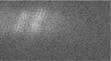
Figure 2: W band cylindrical equal-area projection of the Galactic Centre using 199 days of the 2002 WMAP TOD (Sect. 2.1), compiled using a minor modification of Liu et al. (2010)’s analysis script (Sect. 2.2), for a fractional timing offset $\delta_{t}=-5$ (i.e. an offset of $-256$ ms relative to that of Liu et al.). Galactic latitude increases upwards, galactic longitude increases to the left. The image size is $5.8^{\circ}\times 1.7^{\circ}$, centred at the Galactic Centre. Individual pixels are 1.7^′ in side length. The temperature-fluctuation grey scale ranges from black (-20 mK) to white (+40 mK).

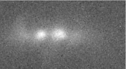
Figure 3: Image of the Galactic Centre, as in Fig. 2, for a fractional timing offset $\delta_{t}=0$ (proposed by Liu et al. 2010).

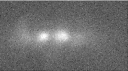
Figure 4: Image of the Galactic Centre, as per Fig. 2, for a fractional timing offset $\delta_{t}=0.5$ (WMAP collaboration value).

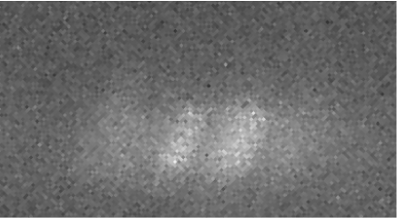
Figure 5: Image of the Galactic Centre, as per Fig. 2, for a fractional timing offset $\delta_{t}=5$.

Nevertheless, the blurring effect should be statistically detectable in maps compiled from the TOD. The effect should be strong if the timing error is exaggerated beyond that proposed by Liu et al. (2010). By considering the timing offset as a free parameter, it should be possible to find the value that minimises blurring. This should correspond to the correct choice of timing interpolation. In principle, since a timing error also induces an error in absolute sky position, this could also be used to determine the correct method. However, it is conceivable that a positional offset may have been at least partially removed at some stage in the pointing calibration, making it hard to detect, as suggested by Moss et al. (2010). On the other hand, a blurring effect is unlikely to have been removed at any step in the production of WMAP maps. Hence, the analysis here uses the blurring effect. In Sect. 2, an empirical method of estimating the blurring using all-sky maps is presented. Images of some Galactic Centre objects as a function of timing offset and the results of the statistical analysis are presented in Sect. 3. Conclusions are given in Sect. 4.

2 Method

2.1 Observational data files and differencing assemblies

Compilation of TOD into maps requires a moderately heavy usage of RAM, CPU and disk space on present-day desktop computers. For this reason, only a subset of the available WMAP TOD is used rather than the full TOD. From each of the years 2002, 2003 and 2004, the files for the first (by filename) 199, 199, and 198 days, respectively, of filtered, calibrated TOD are used, i.e. slightly over six months of data during each year. This allows a convenient filename pattern. Liu & Li (2009) analysed the unfiltered, calibrated, 5-year WMAP data release. The filtering should not significantly affect the questions of interest here.

The primary analysis is done here using the W band, since this has the best resolution. There are four W differencing assemblies (DA’s), giving 12 TOD sets that in many ways can be considered to constitute independent observations. Complementary analyses using the Q and V DA’s, with 6 TOD sets each, are also carried out.

2.2 Compilation of the TOD

Liu et al. (2010) have made their script for compiling the TOD publicly available. For the purposes of the present analysis, minor modifications of this script and associated libraries have been made in order to run the script using the GNU Data Language (GDL). In particular, the data flag parameter daf_mask has been set to 1 in order to include all planet observations when compiling the TOD, and the processing mask has been set to 0 in order not to hide any bright objects from the analysis.

Moreover, the center parameter for determing the timing offset is generalised to an arbitrary floating point value. Here, this is written $\delta t$, i.e. the timing offset expressed as a fraction of an observing time interval in a given band. This is used as a fraction for interpolation between quaternions. Thus, $\delta t=0$ is Liu et al. (2010)’s primary hypothesis of what is the correct offset, and $\delta t=0.5$ is what the WMAP collaboration believes to be correct. In the W band, $\delta t=0$ corresponds to $-25.6$ ms relative to $\delta t=0.5$. In order to reduce computational time, map iteration is not done.

The planets are useful for this analysis because of their high brightness. However, some of them (especially Jupiter) move by up to a few degrees during the times when they happen to be scanned. In directions orthogonal to their movement, a blurring effect is to be expected for a wrong choice of timing offset. In directions parallel to their movement, a wrong choice of timing offset can either cause blurring, or cause some observations that should be mapped to different pixels to incorrectly be mapped to the same pixel, i.e. creating a false focussing effect. The degree to which the latter effect is important depends on the degree to which the observations of a given planet are discontinuous and the way that this discretisation interacts with the scanning pattern directions. In practice, semi-quantitative examination of images of Jupiter suggests that the false focussing effect is present, but weak, for some values of $\delta t$. An analysis using Jupiter alone would need to take this effect into account.

2.3 Pixel resolution and the blurring effect

Since the blurring effect expected from a 25.6 ms timing error would be on a scale of $\sim 4.0$^′, the commonly used HEALPix resolution (Górski et al. 1999) of $N_{\mathrm{side}}=512$ would be insufficient, since this gives pixel sizes of 6.9^′. However, very high resolutions would give very large file sizes. As a compromise, $N_{\mathrm{side}}=2048$ is adopted here, giving a pixel size of 1.7^′ and one-dimensional FITS binary table file sizes of about 190 Mib, or two-dimensional FITS image file sizes of about 400 Mib, using the the HEALPix ($H=4,K=3$) spherical projection (Roukema & Lew 2004; Calabretta & Roukema 2007; Górski et al. 2005). The utility program HPXcvt from the WCSLIB library can be used to convert from one-dimensional to two-dimensional formats. Image files that use the HEALPix spherical projection can be viewed using standard astronomical FITS image viewing tools for visual checking of the blurring effect.

Figures 2–5 show the Galactic Centre from the 2002 WMAP TOD compiled as discussed above, for $\delta_{t}=-5,0,0.5,$ and $5$. Figures 3 and 4 show the timing options of Liu et al. (2010) and the WMAP collaboration, respectively. The blurring effect is not obvious by visual inspection. These two images appear about equally sharp. In contrast, Figs 2 and 5, in which the timing offsets are greater, clearly show both a positional offset and blurring.

2.4 Temperature-fluctuation distribution percentiles

The blurring in Figs 2 and 5 is the key to the method used here. The numbers of very bright pixels in these two figures are much lower than in Figs 3 and 4. This suggests a statistic to characterise the degree of sharpness of the image: the number of pixels $N_{\mathrm{b}}(\delta T/T,\delta t)$ above a given temperature fluctuation threshold $\delta T/T$ in a map calculated at a given timing offset $\delta t$. Maximising $N_{\mathrm{b}}$ over $\delta t$ should give the map most likely to be correct.

The brighter the threshold $\delta T/T$, the fewer the number of pixels that will lie above this threshold, increasing Poisson noise. Thus, fainter thresholds $\delta T/T$ should give stronger signals.

The situation for intermediate brightness pixels is less simple. The signal in the very bright pixels in Figs 3 and 4 has been spread out into intermediate brightness pixels in Figs 2 and 5, increasing the numbers of the latter. However, the signal in regions of intermediate brightness in Figs 3 and 4 has also been blurred out of the same brightness interval, down to fainter levels. For typical profiles of astronomical objects, the number of pixels in each different brightness range should increase as the threshold decreases while remaining well above zero. Hence, the loss of pixels that become blurred below a given threshold $\delta T/T$ should outweigh the gain in pixels from intrinsically higher brightnesses. That is, in general, an incorrect value of the fractional timing offset $\delta t$ should decrease $N_{\mathrm{b}}$ at any positive value of $\delta T/T\gg 0$.

Table 1: Percentile noisiness: mean of $\sigma_{s_{p}}$ (over $\delta t$) in the W band.

$$\begin{array}[]{c cc ccc}\hline\cr\rule[-6.45831pt]{0.0pt}{19.37494pt}p&99\%&99.9\%&99.99\%&99.999\%&99.9999\%\\ \langle\sigma_{s_{p}}\rangle_{\delta t}&0.056&0.041&0.038&0.023&0.051\\ \hline\cr\end{array}$$

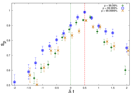
Figure 6: Mean normalised temperature-fluctuation percentiles $s_{p}=\left<s_{p}^{i}\right>$ [Eq. (2)] in compilations of W band WMAP TOD, for pixel fractions $p=99.99\%,99.999\%,$ and $99.9999\%,$ as a function of fractional timing offset $\delta t$. The values $\delta t=0$ and $\delta t=0.5$, favoured by Liu et al. (2010) and the WMAP collaboration, respectively, are shown as vertical lines. The error bars are standard errors in the mean $\sigma_{s_{p}}$ over the 12 DA/year combinations. For clarity, offsets in $\delta t$ of $\pm 0.05$ are applied to the $p=99.99\%$ ($+$) and $99.9999\%$ ($\times$) data points.

Approaching low (positive) temperature-fluctuation levels, the measurement noise in $\delta T/T$ should proportionally increase, so that noise in $N_{\mathrm{b}}$ increases. The effects of smoothing with negative fluctuations will also arise at low positive temperature-fluctuation levels, reducing the effectiveness of testing $N_{\mathrm{b}}$. Hence, the least noisy threshold $\delta T/T$ for optimising the sharpness of images in the map should lie somewhere between the extremes of low positive $\delta T/T$ and high $\delta T/T$.

Rather than choosing fixed values of $\delta T/T$ and studying $N_{b}(\delta T/T,\delta t)$, the approach adopted here is to consider $\delta T/T(pN,\delta t)$, where $p$ is a fraction close to unity and $N=12(2048)^{2}$ is the number of pixels. That is, the percentiles of the (sorted) temperature-fluctuation distribution are determined for several values of $p$, as a function of the fractional timing offset $\delta t$.

Use of different DA’s and different (half-)years of data should give estimates of the random error at any given $p$ and $\delta t$. Averaging over $\delta t$ at a given $p$ makes it possible to find the fraction $p$ that gives the least noisy percentile. Thus, at a given DA and year combination $i$ and a percentage $p\,\lower 2.58334pt\hbox{$\buildrel<\over{\sim}$}\,1$, the percentile is a function

$$\left(\frac{\delta T}{T}\right)_{p}^{i}\,(\delta t).$$ (1)

In order to give approximately equal weight to the different samples $i$, the percentiles are normalised over $\delta t$ internally within each sample $i$ at each $p$. That is, $\left({\delta T}/{T}\right)_{p}^{i}$ is evaluated on a series of maps calculated for $-5\leq\delta t\leq 5$, attaining a minimum $a_{p}^{i}$ and a maximum $b_{p}^{i}$. This is normalised to

$$s_{p}^{i}(\delta t):=\frac{\left({\delta T}/{T}\right)_{p}^{i}(\delta t)-a_{p}^{i}}{b_{p}^{i}-a_{p}^{i}}$$ (2)

The mean and standard error in the mean of $s_{p}^{i}$ over the DA/year combinations $i$ can then be estimated at each $\delta t$. These are written $s_{p}$ and $\sigma_{s_{p}}$, respectively.

3 Results

3.1 W band

Calculations on 4-core, 2.4 GHz, 64-bit processors with 4 Gib RAM, using GDL-0.9$\sim$rc4 running under GNU/Linux, took about 3 hours per map. Table 1 lists the mean of $\sigma_{s_{p}}(\delta t)$ at several values of $p$ for the W band analysis. This shows that $p=99.999\%$, i.e. the fraction $p$ which selects the $\approx$ 503-rd brightest pixel in any given map, gives the least noisy percentile. Figure 6 shows the mean normalised temperature-fluctuation percentiles $s_{p}$ for this and two other values of $p$. The $s_{99.999\%}$ threshold shows a sharp maximum at $\delta t=0.5$. The higher percentile, i.e. at $p=99.9999\%$, is noisier, but still significantly favours $\delta t=0.5$ over any other value of $\delta t$ evaluated. The $p=99.99\%$ percentile is also noisier than that at $p=99.999\%$, and marginally favours $\delta t=0.75$ over $\delta t=0.5$. Liu et al. (2010)’s hypothesis of $\delta t=0$ is not favoured at any fraction $p$.

Exact symmetry around the correct value of $\delta t$ is not necessarily expected, since the scan paths are curved (non-geodesic) paths on the 2-sphere, not straight lines in the 2-plane, and the source objects are not isolated from one another. However, approximate symmetry can reasonably be expected. It is obvious that Fig. 6 is not symmetric around $\delta t=0$. Hiding the part of the figure to the left of $\delta t=-1$ shows that the figure does appear to be approximately symmetric around $\delta t=0.5$.

Table 2: Mean difference in temperature-fluctuation percentiles $\Delta(\delta t^{\prime}):=\left<\;(\delta T/T)_{p}(\delta t=0.5)-(\delta T/T)_{p}(\delta t^{\prime})\;\right>$ for 6 DA/year combinations in each of the Q and V bands in mK, where $p=99.999\%$, and standard error in the mean and significance level.^a

$$\begin{array}[]{ccc cccc }\hline\cr\rule[-6.45831pt]{0.0pt}{19.37494pt}\mathrm{band}&&\Delta(\delta t^{\prime}=0)&\Delta(0.167{{}^{\mathrm{b}}})&\Delta(0.25{{}^{\mathrm{c}}})&\sigma_{\Delta}&\Delta/\sigma_{\Delta}\\ \hline\cr\rule[-6.45831pt]{0.0pt}{19.37494pt}Q&&1.44&-&-&0.05&29\\ Q&&-&-&0.44&0.08&5.5\\ V&&0.70&-&-&0.06&11.7\\ V&&-&0.28&-&0.06&4.8\\ \hline\cr\end{array}$$

^aThe time offsets $\delta t$ and $\delta t^{\prime}$ are in units of one observing interval, i.e. 102.5 ms or 76.8 ms for Q or V, respectively.
^bA shift of $-25.6$ ms relative to the WMAP collaboration choice in the V band.
^cA shift of $-25.6$ ms relative to the WMAP collaboration choice in the Q band.

A quantitative estimate of a lower limit to the significance to which the $\delta t=0$ hypothesis can be rejected, given that it must maximise $s_{p}(\delta t)$, can be obtained by testing the hypothesis that $s_{p}^{i}(\delta t=0)\geq s_{p}^{i}(\delta t=0.5)$ under the assumption that the error distributions are Gaussian. That is, the hypothesis that that a $-25.6$ ms offset relative to the timing adopted by the WMAP collaboration gives a focus at least as sharp as that obtained using the latter’s timing choice is tested. The percentiles shown in Fig. 6 are $s_{p}(0)=0.901\pm 0.019$ and $s_{p}(0.5)=0.989\pm 0.005$, where $p=99.999\%$, i.e. where $s_{p}$ is the percentile that gives the least noisy result, so the hypothesis is rejected at 4.6$\sigma$ significance.

3.2 Q and V bands

A small number of maps were calculated in the Q and V bands, which have lower angular resolution and fewer numbers of DA’s. Only a few maps were calculated, so the percentiles are not normalised. Instead, their differences are calculated. The Liu et al. (2010) hypothesis may be interpreted in the Q and V bands either as a fractional time offset $\delta t=0$ (where $\delta t=0.5$ is the WMAP collaboration’s choice), or as a fixed offset in time units of $-25.6$ ms, since this is the undocumented difference between the start times in the Meta Data Set and the Science Data Set in the TOD files. The latter difference should be more difficult to test than the former, since the interval is smaller in both cases. These differences are calculated individually in each DA/year combination. Table 2 shows their statistics. The weaker form of Liu et al. (2010)’s hypothesis is rejected at very high significance ($\geq 4.8\sigma$) in all cases. In other words, the temperature fluctuation in the $\approx$503-rd brightest pixel is lower for Liu et al. (2010)’s hypothesised offset compared to its value for the WMAP collaboration’s hypothesised offset at very high significance in all cases.

4 Conclusion

The difference in image sharpness for Liu et al. (2010)’s and the WMAP collaboration’s respective timing interpolation choices are not obvious in the images of the Galactic Centre shown in Figs 3 and 4. However, use of the all-sky images gives estimates of image sharpness that depend strongly on the fractional time offset $\delta t$. These calculations do not require any fitting of source or beam profiles, nor any selection of one or more preferred sources, nor any assumptions regarding pointing accuracy. The data analysis pipeline is performed using Liu et al. (2010)’s script, with only minor modifications, on slightly under a quarter of the full set of WMAP calibrated, filtered TOD. Liu et al. (2010)’s timing error hypothesis is rejected at very high significance in the Q, V and W wavebands separately.

The lack of an explanation in the WMAP Explanatory Supplement (Section 3.1, Limon et al. 2010) for the 25.6 ms offset between the start times in the Meta Data Set and the Science Data Set in the TOD files is an unfortunate gap in the documentation, but it clearly did not lead to an error of this magnitude in the WMAP collaboration’s compilation of the calibrated, filtered TOD. A possible explanation for the offset could be that it is a convention inserted by software into the Meta Data Set that was forgotten about, rather than a physical time offset. In principle, it would be good if the WMAP collaboration could find the line(s) in their software where the 25.6 ms offset is inserted, in order to confirm that its origin is fully understood, and that it has no unintended consequences.

Nevertheless, the fact that Liu & Li (2009) accidentally applied a time offset that approximately cancels the $\delta t=0.5$ CMB quadrupole in amplitude and direction, and that this can be modelled as a Doppler-dipole-induced difference signal (Eq. (2), Liu et al. 2010, “deviation of differential dipole”), remain interesting coincidences. The relations between the quadrupole, octupole and ecliptic (e.g., Copi et al. 2006; Sarkar et al. 2010) have long been known. What remains unestablished is whether these are coincidences or artefacts. Moss et al. (2010) discuss the possibility of relationships between the various coincidences and suggest that another effect might couple with the WMAP spacecraft velocity dipole in order to produce an artificial component of the quadrupole.

One interesting possibility for further work would be to consider a variation on the hypothesis proposed by Liu et al. (2010): could it be possible that the would-be timing error was introduced when calibrating the uncalibrated TOD? Although the velocity dipole is only removed from the data during the mapmaking step, it is first used for calibrating the raw data into a calibrated signal in mK. So, a small timing error during the calibration step could correspond to artificially adding a dipole-induced difference signal. During the following step of compiling the calibrated TOD into maps, the dipole would then be subtracted at the correct positions, but without compensating for the incorrect calibration. As noted above, Jarosik et al. (2007) (Sect. 2.4.1) have earlier considered the possibility that a calibration error (not necessarily induced by a timing error) could introduce an artificial, dipole-induced quadrupole.

The calibration method for the 7-year WMAP analyses are stated (Jarosik et al. 2010) to be those used for the 5-year analyses, i.e. as described in Sect. 4 of Hinshaw et al. (2009), retaining the estimate of about 0.2% absolute calibration error. Since the dipole amplitude is about 3 mK, a 0.2% error corresponds to about 6 $\mu$K. The 7-year quadrupole estimated for $\delta t=0.5$ is $\sqrt{(3/\pi)C_{2}}\approx 14\mu$K (Section 4.1.1, Jarosik et al. 2010), only a factor of two higher than this calibration uncertainty (though the model-dependent systematic error is high for the infinite flat model). Liu & Li (Sect. 4, Fig. 6, 2009) estimate the quadrupole-like difference between their Q1 DA $\delta t=0$ map and the WMAP collaboration’s $\delta t=0.5$ map to have an r.m.s. of 6.6 $\mu$K. Moreover, the spacecraft’s velocity is assumed by Hinshaw et al. (2009) and Jarosik et al. (2010) to be known exactly, and fits are made over intervals “typically between 1 and 24 hours”. It is not obvious that a timing error causing the spacecraft’s velocity vector to be slightly misestimated, which in turn causes a quadrupole-like dipole-induced difference signal over a year’s observations, of amplitude $\sim 5$–$10\mu$K, would have been detected or removed during the calibration process. Indeed, Cover (2009) claims the presence of considerable systematic uncertainty in the calibration of the WMAP TOD.

The calibration only applies to (differential) radio flux density estimates, not to positional data, so it would not affect the latter, i.e. the spacecraft attitude quaternions. The Meta Data Tables containing the quaternions appear to be identical between the “uncalibrated” and “calibrated, filtered” WMAP 3-year TOD files, as can be expected. Hence, an incorrect calibration that leads to a dipole-induced difference signal would not cause an arcminute-scale blurring effect nor a positional error in point sources. It would not be detectable by the method used in this paper. Since a large fraction of the brightest point sources at WMAP frequencies are variable, it may not be easy to use point sources to calibrate the uncalibrated data independently of the dipole calibration. Liu & Li (2009) and Liu et al. (2010) appear to use the word “raw” to refer to the calibrated (filtered for 3-year analyses, unfiltered for 5-year analyses) TOD and do not appear to have carried out the calibration step.

Independently of these considerations, the correct way to compile the calibrated WMAP TOD into sky maps must clearly be the one that optimises the sharpness of the images of bright sources. Whether or not the calibration step itself was carried out with a small timing error—leading to an artificial dipole-induced difference signal—remains to be investigated. Liu et al. (2010)’s calculations suggest that the latter is an interesting possibility.

Appendix A Time offset between Meta Data Table and Science Data Table

Since the time offset between the Meta and Science Data Tables in the WMAP TOD has escaped attention for many years, a method of verifying this is provided here.

The TOD files, the GNU Data Language (GDL), and the IDL Astro library are available at http://lambda.gsfc.nasa.gov/product/map/dr2/ tod_fcal_get.cfm,
http://idlastro.gsfc.nasa.gov/ftp/astron.dir.tar.gz, http://gnudatalanguage.sourceforge.net/, respectively. The file path for the IDL Astro library can be set up using the equivalent of

 cd pro && ln -s */*.pro . && export GDL_PATH=‘pwd‘

in a bash shell. The line

ndata = product( axis, /integer )

in the IDL Astro routine fits/fits_read.pro should be replaced by

      ndata = floor( product( axis ) + 0.5)

for use in GDL-0.9$\sim$rc3 or earlier. The following GDL script demonstrates the timing offset in the TOD, where “tod.fits” is the name of a TOD file.

pro TOD_offset
  fits_open, ’tod.fits’, handle
  ;; get table of times (metatime) of quaternions
  ;; of spacecraft attitude
  fits_read, handle, metatable, metaheader, $
             extname = ’Meta Data Table’
  tbinfo, metaheader, meta_h
  metatime= tbget(meta_h,metatable,’Time’)

  ;; get table of times (scitime) stored in table
  ;; that includes observational data
  fits_read,handle,scitable,sciheader, $
            extname = ’Science Data Table’
  tbinfo,sciheader,sci_h
  scitime= tbget(sci_h,scitable,’Time’)

  ;; re-interpret 1D table as 2D table
  scitime0=reform(scitime,30,1875)
  ;; calculate the offsets in seconds
  offset = (metatime - scitime0[0,*]) *3600d *24d

  ;; print some examples
  print,’quaternion time minus data time in s: ’+ $
        ’first 10 frames of the day’
  print,offset[0:9],format="(d15.7)"
  print,’quaternion time minus data time in s: ’+ $
        ’last 10 frames of the day’
  print,offset[1865:1874],format="(d15.7)"
  print,’mean and stand. deviation:’
  print,mean(offset),format="(d15.12)"
  print,sqrt(mean((offset-0.0256)^2)), $
        format="(d15.12)"
end