Finite temperature QMC study of the one-dimensional polarized Fermi gas

Abstract

Quantum Monte Carlo (QMC) techniques are used to provide an approximation-free investigation of the phases of the one-dimensional attractive Hubbard Hamiltonian in the presence of population imbalance. The temperature at which the “Fulde-Ferrell-Larkin-Ovchinnikov” (FFLO) phase is destroyed by thermal fluctuations is determined as a function of the polarization. It is shown that the presence of a confining potential does not dramatically alter the FFLO regime, and that recent experiments on trapped atomic gases likely lie just within the stable temperature range.

I Introduction

Pair formation between fermions is one of the most rich and active fields of investigation in condensed matter systems, occuring in contexts as varied as exciton formation in quantum well structures golub to its most well-studied realization, the superconducting state BCS . Indeed, the possibility of pair formation has many even wider implications, including the early speculation that it might dominate the nature of interior of neutron stars ginzburg . By far the most commonly studied situation is one in which the populations of the two fermion species (normally up and down spins) are balanced, and Cooper pairs form with zero center of mass momentum cooper . Soon after the development of the BCS theory BCS of superconductivity, the question of pair formation in polarized superconducting systems, i.e. when the populations of the two spin states are imbalanced, was addressed independently by Fulde and Ferrel fulde (FF), Larkin and Ovchinnikov larkin (LO) and Sarma sarma . The question was motivated by interest in the nature of superconductivity in the presence of a magnetic field, which induces spin polarization.

FF and LO (henceforth FFLO) proposed similar, yet not identical, mechanisms whereby the Cooper pairs form with non-zero center of mass momentum equal to the difference of the now-unequal Fermi momenta of the two species. As a consequence, in the FFLO scenario the order parameter is not homogeneous; the system has pair-rich regions separated by regions depleted in pairs but with an excess of the majority, unpaired fermion species. In the competing proposal by Sarma, the Fermi surfaces deform to allow pair formation with zero center of mass momentum. This means that the system remains uniform; it is a homogeneous mixture of pairs and unpaired fermions from the majority population. In other words, in the FFLO mechanism, the momentum distribution of pairs has its peak at a momentum equal to the difference between the two Fermi momenta, $k_{\rm peak}=|k_{F1}-k_{F2}|$. On the other hand, the Sarma mechanism would result in a pair momentum distribution with $k_{\rm peak}=0$. Deciding between these two scenarios experimentally proved to be very difficult; the observation of the FFLO phase in solids was only achieved relatively recently in heavy fermion systems radovan03 .

This question has recently taken on added importance. Interest in the astrophysical community has continued to grow and broaden. It is now believed that at extreme conditions of pressure, for example in the interior of supermassive stars, quark matter forms and pairing between the quarks could lead to color superconductivity Casalbuoni . More immediate experimental systems where these effects may be observed, and are indeed sought, are ultra-cold atoms confined in traps where two hyperfine states of fermionic atoms play the role of up and down spins. Such experiments have now reported the presence of pairing in the case of unequal populations zwierlein06 ; partridge06 in three-dimensional cigar shaped traps and in one dimensional traps hulet . However, the precise nature of the pairing has not yet been elucidated experimentally.

On the theoretical side, much effort has been put into understanding the pairing mechanism. Calculations using mean field theory castorina05 ; sheehy06 ; kinnunen06 ; machida06 ; gubbels06 ; parish07 ; hu07 ; he07 ; wilczek ; koponen ; Drummond1 , effective Lagrangian son06 and Bethe ansatz orso studies have been performed for the uniform system, with extensions to the trapped system using the local density approximation (LDA). Extensive numerical work for the one dimensional system using Quantum Monte Carlo (QMC) batrouni08 ; casula , and the Density Matrix Renormalization Group (DMRG) feiguin07 ; luscher ; rizzi ; tezuka07 ) has demonstrated that, in the ground state, population imbalance leads to a robust FFLO phase over a very wide range of polarization and interaction strengths.

In addition to the above case of population imbalance, the case of mass imbalance has been addressed theoretically wilczek1 ; wilczek2 and numerically batrouni09 . This case is relevant to color superconductivity, where the quark masses are not equal, and also to ultra-cold ⁴⁰K-⁶Li atomic mixtures.

The stability of the FFLO phase at finite temperatures remains an open question. Mean field calculations KoponenfiniteT ; DrummondfiniteT ; Kakashvili possibly shed some light but can be less reliable in low dimension where quantum fluctuations are large. This question is of paramount importance for experiments, especially in trapped atomic systems, since difficulties in cooling fermionic atoms raise concerns about whether the currently attainable temperatures are low enough for a thorough investigation of FFLO physics. The present paper reports on QMC studies of this issue which provide an exact treatment of interaction effects on lattices of finite size. The key result is that, when the polarization is sufficiently large, the paired phase can exist up to temperatures of order one tenth of the Fermi energy, even in the presence of a confining potential. Current experiments on trapped atoms are likely in this temperature range.

The paper is organized as follows. In the next section we will discuss the model and the numerical methods used. In section III, we discuss our results for the phase diagram of the uniform one-dimensional system at finite temperature. In section IV we discuss the trapped one dimensional system followed by our conclusions in section V.

II Model and Methods

In order to study the pairing mechanism of fermions in an optical lattice, we consider the one-dimensional fermionic Hubbard Hamiltonian,

$$H = -t\sum_{i\,\sigma}(c_{i\,\sigma}^{\dagger}c_{i+1\,\sigma}^{\phantom{\dagger}}+c_{i+1\,\sigma}^{\dagger}c_{i\,\sigma}^{\phantom{\dagger}})-\sum_{i}(\mu_{1}\hat{n}_{i\,1}+\mu_{2}\hat{n}_{i\,2})$$ (1)

$$+U\sum_{i}\left(\hat{n}_{i\,1}-\frac{1}{2}\right)\left(\hat{n}_{i\,2}-\frac{1}{2}\right)$$

$$+V_{T}\sum_{i}\left(x_{i}-\frac{L}{2}\right)^{2}\left(\hat{n}_{i\,1}+\hat{n}_{i\,2}\right)$$

where $c_{i\,\sigma}^{\dagger}$ and $c_{i\,\sigma}^{\phantom{\dagger}}$ are fermion creation and annihilation operators on lattice site $i$ satisfying the usual anticommutation relation, $\{c^{\phantom{\dagger}}_{i\,\sigma},c^{\dagger}_{j\,\sigma^{\prime}}\}=\delta_{i,j}\delta_{\sigma,\sigma^{\prime}}$. The fermionic species are labeled by $\sigma=1,2$ and $\hat{n}_{i\,\sigma}=c_{i\,\sigma}^{\dagger}c_{i\,\sigma}^{\phantom{\dagger}}$ is the corresponding number operator. The energy scale is set by taking the hopping parameter $t=1$. The contact interaction strength is $U$ which is negative since we are interested in pair formation in the attractive model. In the grand canonical ensemble, the populations are fixed by tuning the chemical potentials for the two species, $\mu_{1}$ and $\mu_{2}$, whereas in the canonical ensemble this term is absent and the populations are fixed simply by choosing the number of particles. As we discuss below, both ensembles will be used in this work. The last term describes the confining harmonic trap which is centered at the midpoint, $L/2$, of the $L$-site lattice. We take periodic boundary conditions.

Our Quantum Monte Carlo (QMC) results are obtained using two different methods: the Determinant QMC algorithm DQMC (DQMC) and the Stochastic Green Function (SGF) technique SGF ; DirectedSGF . In DQMC, the interaction term in the Hamiltonian, which is quartic in the fermionic operators, is decoupled via the Hubbard-Stratonovich (HS) transformation. This allows the fermion operators to be traced out, giving an expression for the partition function as an integral over the configurations of the auxiliary HS field. We employ the grand canonical formulation of DQMC. The statistical weight of these configurations is given by the product of the spin up and down determinants, each of which can change sign depending on the HS configuration. When the populations are balanced, $\mu_{1}=\mu_{2}$, it is well known that DQMC does not suffer from the sign problem for an attractive interaction ($U<0$): The two determinants are identical and thus their product is always positive. This is no longer the case when the populations are imbalanced, $\mu_{1}\neq\mu_{2}$ (or for $U>0$), resulting in the appearance of the sign problem. The severity of this problem depends on several factors such as the size of the system, the coupling constant, the temperature and the imbalance in the populations. For the systems and parameters we consider in this work (see below) the average sign did not fall below $0.5$, which allowed us to obtain good statistical precision in our simulations. We used this algorithm for the uniform system; it has the advantage of rather fast convergence rates, but to perform simulations at fixed particle numbers, the chemical potentials need to be tuned. A typical simulation for $L=50$ sites and $\beta=30$ with an imaginary time step $\Delta\tau=0.1$ runs for about $4$ to $5$ days on a desktop computer and yields error bars of the order of $0.5\%$ for the peak of the pair momentum distribution, a central quantity of interest in this work.

The SGF algorithm SGF with directed update DirectedSGF can be used both in the grand canonical or canonical modes. We describe it in more detail than DQMC since it has been developed much more recently. First, the Hamiltonian is written as $H=\hat{\cal V}-\hat{\cal T}$, where $\hat{\cal V}$ is diagonal in the occupation number basis of the direct space, and $\hat{\cal T}$ is the remaining non-diagonal part. The algorithm samples an extended partition function represented in the interaction picture,

$${\cal Z}(\beta,\tau)={\rm Tr}\,e^{-\beta\hat{\cal V}}T_{\tau}\Big{[}\hat{\cal G}(\tau)e^{\int_{0}^{\beta}\hat{\cal T}(\tau)d\tau}\Big{]},$$ (2)

where $T_{\tau}$ is the time-ordering operator and the time dependence of any operator $\hat{\cal A}(\tau)$ is given by the interaction representation $\hat{\cal A}(\tau)=e^{\tau\hat{\cal V}}\hat{\cal A}e^{-\tau\hat{\cal V}}$. The “Green operator” $\hat{\cal G}$ is defined by its matrix elements, $\big{\langle}\psi_{L}\big{|}\hat{\cal G}\big{|}\psi_{R}\big{\rangle}=g_{pq}$, where $p$ and $q$ are the number of creations and destructions of particles that transform the (occupation number) state $\psi_{R}$ into $\psi_{L}$. The matrix $g_{pq}$ is a decreasing function of $(p+q)$ SGF . The extended partition function (2) is expanded in $\hat{\cal T}$ yielding operator strings of the form:

$$\cdots\hat{\cal T}(\tau_{L+2})\hat{\cal T}(\tau_{L+1})\hat{\cal T}(\tau_{L})\hat{\cal G}(\tau)\hat{\cal T}(\tau_{R})\hat{\cal T}(\tau_{R-1})\hat{\cal T}(\tau_{R-2})\cdots,$$ (3)

The Green operator updates the operator string (3) by propagating in imaginary time, while inserting and removing $\hat{\cal T}$ operators. From its definition, the Green operator contains terms that do not conserve the number of particles. However if the Hamiltonian commutes with the operator that measures the total number of particles, $\hat{\cal N}$, for example the Hamiltonian (1), then only conservative terms of $\hat{\cal G}$ have non vanishing contributions since the trace imposes the same number of particles both at the begining and the end of the operator string. As a consequence the number of particles remains strictly constant and the SGF algorithm works in the canonical ensemble by nature. However, a simple trick can be used in order to simulate exactly the grand-canonical ensemble. The idea is to add a non conservative part $\hat{\cal H}_{\textrm{nc}}$ to the Hamiltonian,

$$\hat{\cal H}_{\textrm{nc}}=\gamma\sum_{j}\big{(}a_{j}^{\dagger}+a_{j}^{\phantom{\dagger}}\big{)},$$ (4)

where $\gamma$ is an optimization parameter, and allows the Green operator to insert at most one $\hat{\cal H}_{\textrm{nc}}$ operator in the string. This allows the number of particles to fluctuate, while the addition of the usual term $-\mu\hat{\cal N}$ to the Hamiltonian determines the mean number of particles via the chemical potential $\mu$. When measuring physical quantities, ignoring configurations in which the operator string contains a $\hat{\cal H}_{\textrm{nc}}$ operator, corresponds to integrating over these configurations the probability of going from a given configuration with $N$ particles and no $\hat{\cal H}_{\textrm{nc}}$ to another one with $M$ particles and no $\hat{\cal H}_{\textrm{nc}}$, via intermediate configurations with $\hat{\cal H}_{\textrm{nc}}$. This integrated probability corresponds exactly to the probability of going from one configuration with $N$ particles to another one with $M$ particles. As a result, the configurations of the grand-canonical partition function $\textrm{Tr }\,e^{-\beta(\hat{\cal H}-\mu{\hat{N}})}$ are generated with the correct Boltzmann weight.

To use this algorithm to simulate fermions in one dimension, we first use the Jordan-Wigner transformation to map the system onto a system of hard core bosons. Consequently, this algorithm does not suffer from the sign problem but, clearly, it cannot be used in higher dimensions where the Jordan-Wigner transformation fails to solve the sign problem. We used this algorithm in the canonical ensemble mainly for the confined system where it is very convenient to control the populations directly rather than tune the chemical potentials. A typical simulation for $L=120$ and $\beta=32$ runs for about $5$ days on a desktop computer and yields an error of the order of $0.5\%$ for the peak of the pair momentum distribution..

As part of our code verification, the grand canonical SGF and DQMC were compared for the same parameters and found to yield the same results within the error bars. Furthermore, we verified that DQMC and grand canonical SGF both agreed with the canonical SGF when the chemical potentials in the grand canonical cases were tuned to give the same populations as the canonical cases, see for example Ref.[batrouni08, ]. The results presented below were obtained with these three algorithms; the choice being dictated by the specific measurement we were after. Because of the equivalence of the three algorithms, we will not comment below on which results were obtained with which algorithm.

Using these algorithms, we calculate both the real space Green functions of the species, $G_{\sigma}$, and the pair green function, $G_{\rm pair}$,

$$G_{\sigma}(l) = \langle c_{j+l\,\sigma}^{\dagger}c_{j\,\sigma}^{\phantom{\dagger}}\rangle,$$ (5)

$$G_{\rm pair}(l) = \langle\Delta^{\dagger}_{j+l}\,\Delta_{j}^{\phantom{\dagger}}\rangle,$$ (6)

$$\Delta_{j} = c_{j\,2}\,c_{j\,1},$$ (7)

where $\Delta_{j}$ destroys a pair on site $j$. The Fourier transform of $G_{\sigma}(l)$ yields the momentum distributions $n_{\sigma}(k)$ and the transform of $G_{\rm pair}(l)$ leads to the pair momentum distribution, $n_{\rm pair}(k)$, a central quantity in this work. In the non-interacting limit, the Fermi momentum of a population is given by $k_{F\sigma}=\frac{N_{\sigma}-1}{2}\frac{2\pi}{L}$, where $L$ is the length of the system and $N_{\sigma}$ the number of particles.

III Phase diagram of the homogenous system

We begin with a discussion of the physics in the absence of a confining potential, $V_{T}=0.$

As discussed in the introduction, it is now generally agreed that the ground state of a Fermi system with attractive interactions and imbalanced populations is the FFLO state. The mismatch in the Fermi momenta results in pair formation with nonzero center-of-mass momentum $k=\pm|k_{F_{1}}-k_{F_{2}}|$. Consequently the pair momentum distribution, the Fourier transform of the pair Green function Eq.(6), peaks at this value of the momentum. This peak at nonzero momentum serves as the principal diagnostic indicating the presence of the FFLO state batrouni08 ; luscher ; rizzi ; tezuka07 ; feiguin07 .

The situation at finite temperature, which is important experimentally, is less clear. Approximate methods, such as mean field, do not always yield the same phase diagram. In this section we will map out the phase diagram in the polarization-temperature plane where the polarization is defined by,

$$P=\frac{N_{1}-N_{2}}{N_{1}+N_{2}},$$ (8)

where $N_{1}$ ($N_{2}$) is the majority (minority) population and $N=N_{1}+N_{2}$ is the total number of particles. To this end, we study, at fixed $P$, the behaviour of the pair momentum distribution, $n_{\rm pair}(k)$, as a function of the temperature $T$. For very low $T$, $n_{\rm pair}(k)$ peaks at $k\neq 0$ and the system is in the FFLO state. As $T$ is increased, the peak in $n_{\rm pair}$ gets lower and shifts to $k=0$. The temperature at which this first happens is the cross-over temperature, $T_{c}$. Note that in this one-dimensional system, transitions at finite temperature are not true phase transitions, but rather cross-overs.

This is illustrated in Fig. 1 where we show QMC results for $n_{\rm pair}(k)$ as a function of $k$ for several values of the inverse temperature $\beta$. The simulations were done for fixed populations, $N_{1}=13$ and $N_{2}=7$ on a system with $L=32$ lattice sites and an attractive interaction $U=-3.5t$. The figure shows clearly that as $\beta$ decreases from $\beta=32$, the height of the FFLO peak decreases and, in fact, shifts to lower $k$ values. The shift to lower $k$ values is made more evident by simulating larger systems since this gives more $k$ grid points. When the peak at nonzero $k$ is equal to $n_{\rm pair}(0)$ to within $1\%$, we consider the peak to have shifted to $k=0$ and the FFLO state to have disappeared. In the Fig. 1 this happens for $\beta_{c}\approx 6$. Reducing $\beta$ further leads to continued decrease of the height of the peak, which remains at $k=0$.

The question then arises as to how the FFLO peak behaves as a function of $U$ at fixed $\beta$, $N_{1}$ and $N_{2}$ (and consequently fixed $P$). Clearly, for $U=0$ there is no pairing and no FFLO peak; then, as $|U|$ is increased, the peak at nonzero $k$ forms and its height increases. However, we found that as $|U|$ continues to increase, the FFLO peak will reach a maximum height and then start to decrease. We also found that the peak is more sensitive to $|U|$ at higher $T$. We believe the reason the peak starts to go down at high values of $|U|$ is that with increasing attraction, the pairing becomes increasingly localized in space and eventually the paired fermions form a very tightly bound bosonic molecule and the system resembles closely a usual Bose-Fermi mixture which does not exhibit FFLO peaks.

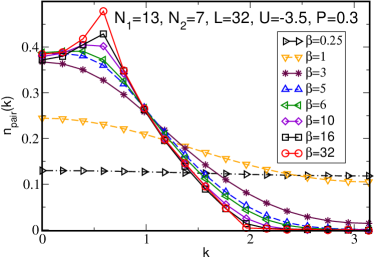
Figure 1: (color online) The effect of temperature on the pair momentum distribution. A peak at non-zero momentum is a signature of the FFLO state. As $\beta$ decreases, the peak disappears at a crossover value $\beta_{c}=1/T_{c}$. In this case, $\beta_{c}\approx 6$. The error bars are of the order of the symbol size.

The peak of $n_{\rm pair}(k)$ at $k_{\rm peak}\neq 0$ means that the system is, in fact, not homogenous: The spatial pair Green function, Eq.(6), oscillates as a function of distance with a period given by $2\pi/|k_{\rm peak}|$. These oscillations have been discussed, for example, in the context of mean field theory Drummond1 ; Trivedi . Physically, they indicate that the system has regions which are rich in pairs separated by regions poor in pairs but rich in the excess fermion species. Such oscillations are shown in Fig. 2 for three values of $\beta$. It is seen that as the temperature increases and the height of the FFLO peak decreases, the oscillations decrease in amplitude and eventually disappear as homogeneity is restored in the system.

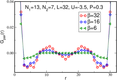
Figure 2: (color online) Pair Green function calculated at low temperatures where the system is in the FFLO state ($\beta=32$ and $\beta=16$) and at the temperature at which FFLO disappears ($\beta=6$). Note that the oscillations disappear at the higher temperature.

The question then arises as to the nature of the phase at $T>T_{c}$. Two possibilities are: (1) At $T>T_{c}$ the pairs are broken and the system is a mixture of two Fermi liquids or (2) pairs are still present but the system has been homogenized by thermal agitation. A first indication is given by the energy scales involved. The binding energy of the pairs at very low temperature is of the order of $|U|$ and in our system here $|U|=3.5t$. So, to break the pairs, an equivalent amount of thermal energy is needed which means $\beta\approx 1/|U|$. For the case discussed in Fig. 2, the crossover from FFLO to the uniform phase happens at $\beta_{c}\approx 6$ not $t/|U|=0.286$. This means that $T_{c}$ is more than an order of magnitude smaller than the temperature needed to break the pairs. This, then, favors the conclusion that when FFLO first disappears, the pairs have not yet been broken and the system is in a homogeneous polarized paired phase (PPP). Another piece of evidence is provided by studying the average double occupancy of the sites given by

$$D=\langle n_{i1}n_{i2}\rangle=\langle\Delta_{i}^{\dagger}\,\Delta^{\phantom{\dagger}}_{i}\rangle.$$ (9)

In the absence of pairing, $\langle n_{i1}n_{i2}\rangle=\langle n_{i1}\rangle\langle n_{i2}\rangle=N_{1}N_{2}/L^{2}$ while if pairing is perfect, i.e. if all the minority particles are paired, $\langle n_{i1}n_{i2}\rangle=N_{2}/L$. We define the normalized double occupancy by

$${\cal D}=\frac{D-n_{1}n_{2}}{n_{2}-n_{1}n_{2}},$$ (10)

where $n_{1}=N_{1}/L$ and $n_{2}=N_{2}/L$ and we recall that $N_{2}<N_{1}$. With this normalization, we have $0\leq{\cal D}\leq 1$. This quantity is shown in Fig. 3 for three polarizations. One can see that the pairing drops significantly at rather high temperatures, $\beta\approx 1/U$. Thus we conclude that the pairs are not broken when the FFLO peak disappears but the systems is in a PPP. As one can see, this pairing parameter does not saturate for the case we presented. One could expect it to reach the maximum value at a very strong U limit in the low temperature regime, where both thermal and quantum fluctuations are absent.

Figure 3: (color online) Double occupancy versus $\beta$ for three polarizations exhibits a very sharp drop for $\beta<1$ indicating that pairs are being broken near $\beta\sim 1/|U|$.

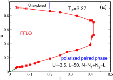
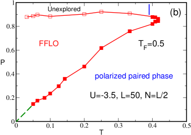
Figure 4: (color online). Phase diagram in the polarization-temperature plane. (a) the system at $N=L$ (half filling), (b) the system at $N=L/2$ (quarter filling). At P=0 system is in the BCS state. The regions above the open (red) squares and to the left of the vertical (blue) lines are unexplored. Up to the open squares the system is in the FFLO phase. Phase boundaries represent cross-over behaviour not phase transitions. In the FFLO phase, $n_{\rm pair}(k)$ peaks at $k\neq 0$, in the PPP phase, the peak is at $k=0$.

We are now ready to apply the above considerations to determine the phase diagram in the $(P,T)$ plane. To this end, we keep the total population, $N$, constant and for different values of the polarization, $P$, determine the temperature, $T_{c}$, at which the peak in $n_{\rm pair}(k)$ shifts to $k=0$. Figure 4 shows the resulting phase diagrams for $N=L$ (half filling) and $N=L/2$ (quarter filling). We mention again that the phase boundaries represent crossover behaviour, not phase transitions since this one-dimensional quantum system does not have phase transitions at finite temperature. The Fermi temperatures shown in the figure are calculated assuming equal populations using $\epsilon_{F}=tk_{F}^{2}$ where $\epsilon_{F}$ is the Fermi energy.

The phase diagrams show clearly that the FFLO phase is quite robust, persisting over a wide range of polarizations and to rather high temperatures. For $N=L$, it persists up to $T/T_{F}\approx 0.2$ and for $N=L/2$ up to $T/T_{F}\approx 0.8$. We also see that, in both cases, the crossover temperature increases with the polarization up to a maximum value after which it decreases again. This can be understood physically as follows: When $P$ is small, the Fermi “surfaces” of the two populations are so close to matching that very little thermal energy is needed to get them to match. Thus even at very low finite temperature, pairing takes place at zero center-of-mass momentum. Therefore, larger polarizations have a stabilizing effect on the FFLO phase.

There are numerical difficulties with the determination of the phase diagram at very low and very high polarizations. At very high polarization, there is a very small number of minority particles, making the FFLO signal difficult to discern clearly. We were therefore not able to examine $P>0.9$ in our simulations. For that reason, some symbols on the phase boundary at high polarization are open, indicating that up to this polarization, the system is in the FFLO phase. The solid symbols demark the true boundary between FFLO and PPP.

In addition, at small polarization, very low temperature is needed to observe the FFLO phase. However, there is a practical limit on how low a temperature we can simulate since the lower the temperature the longer the simulation time needed to obtain precise results. The dashed (green) line connecting the origin to the first numerical points simply schematizes the expected position of the boundary.

A phase diagram in the $(P,T)$ plane was calculated in Ref. koponen using mean field theory (MFT). The general shape of the FFLO phase obtained there (Fig. 9 of Ref. koponen ) is similar to what we found here. However there are very important differences. For example, unlike MFT, we have found that there is no direct transition from the FFLO phase to the Fermi liquid phase (broken pairs): The FFLO phase is destroyed at a temperature which is much lower than that required to break the pairs and is replaced by the PPP.

Reference koponen predicts phase separation between the FFLO and PPP at low $P$ and $T$ (Fig. 9 in Ref. koponen ). In order to examine this possibility, we study the density histograms in the grand canonical ensemble. The idea is as follows: Starting in, say, the PPP, we increase the polarization by tuning the chemical potentials, $\mu_{1}$ and $\mu_{2}$. For each choice of $\mu_{1}$ and $\mu_{2}$, we accumulate the histograms of the particle populations. If phase separation is present, then as the system approaches the phase separation region, the density histogram of each species should develop a double peak structure. If no such structure develops, it means that there is no phase separation as the system crosses from the PPP to the FFLO. We first verify the correct behaviour of the obtained histogram as the size of the system is changed. In Fig. 5 we show the histograms for two system sizes at half filling but with all other parameters fixed. We see that the histograms for the two system sizes agree very well; the main difference is that the larger system size (obviously) allows for a finer grid of densities which redistributes the values a little and exhibits the main peak more clearly. In Fig. 6 we show, for fixed inverse temperature $\beta=16$, the histograms for three cases at half filling: In the top panel the system is just inside the PPP phase, the middle panel the system is at the PPP-FFLO boundary and the bottom panel the system is just inside the FFLO phase. No double peak structure develops, which leads us to conclude that there is no phase separation. This was done for several temperatures at low polarization.

It is useful here to comment on the algorithm choice for calculating the histograms. Although the DQMC algorithm is grand canonical and thus allows for particle number fluctuations, it is not useful for calculating the density histograms. The reason is that in DQMC one changes the realization of the auxiliary Hubbard-Stratonovich field; but for each such realization, the fermions have been traced over all their possible configurations. On the contrary, in the grand canonical version of the SGF algorithm, the update is done over the fermion configurations themselves. So, the particle number can be measured configuration by configuration.

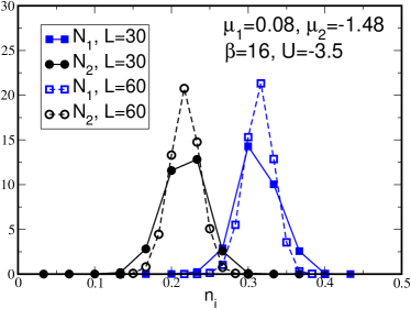
Figure 5: (color online). Majority ($N_{1}$) and minority ($N_{2}$) density histograms at the FFLO-PPP boundary for two system sizes. The larger system size offers more grid points and, therefore, a finer resolution of the density fluctuations. A single peak is seen for each population indicating the absence of phase separation.

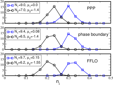
Figure 6: (color online). Histograms of local densities for $L=30$, $\beta=16t$ and $U=-3.5t$. Left peaks correspond to the minority species and right ones to the majority. The peaks move smoothly as $\mu_{1}$ and $\mu_{2}$ are tuned to take the system across the boundary between PPP and FFLO. No double peak structure is observed, indicating the absence of phase separation.

IV Trapped system at finite temperature

Continuing earlier work in higher dimension zwierlein06 ; partridge06 , the Rice group hulet recently reported on experiments in one dimensional confined Fermi systems (${}^{6}Li$ atoms) with imbalanced populations. These experiments were done in the continuum, i.e. without an optical lattice, and focused on the behaviour of the system in three polarization regimes by measuring the density profiles of the fermionic species. It was found that the central part of the system is always partially polarized whereas the behaviour of the outlying regions depends on the total polarization. For low polarization, $P=0.05$, the outlying regions were found to be fully paired in the sense that the density profiles of the two fermion species matched within experimental precision. For medium polarization, $P=0.15$, the density profiles indicated that the whole system is partially polarized. Finally, for large polarization, $P=0.59$, the wings were found to be populated exclusively by the excess fermion species and thus were fully polarized.

The experiment hulet consisted of a two-dimensional array of elongated (one-dimensional) tubes. Along the tube, the axial direction, the atoms were confined with a trap frequency $\omega_{z}=2\pi\times 200$Hz; in the central tube, the total number of atoms at zero polarization was approximately $250$ and the temperature was estimated at $T/T_{F}\approx 0.1$. The pair binding energy, $\epsilon=\hbar^{2}/ma_{1D}$ (where $a_{1D}$ is the effective one-dimensional scattering length), was estimated to be $\epsilon/\epsilon_{F}\approx 5.3$ with the Fermi energy calculated assuming a balanced system with a total of $250$ particles.

In this section, we present QMC results for the fermionic Hubbard model, Eq.(1), in the presence of the confining trap. Our goal is to make contact with the above mentioned experiment in the continuum; to this end we simulate lattice systems that are dilute enough so that the fermions in the center of the trap are far from forming a flat plateau corresponding to a band insulator. We introduce the trapping potential in Eq.(1) $V_{T}=0.0007t$ which corresponds to $\hbar\omega_{z}=2\sqrt{tV_{T}}$. The total number of particles in our simulations for balanced populations is $78$, to be compared with $250$ in the experiment. We performed our simulations in the temperature range $0.008\leq T/T_{F}\leq 0.25$ which includes the temperature at which the experiments were performed, $T/T_{F}=0.1$. In addition, to place our system in the same coupling parameter regime as the experiments, we present our results for a coupling strength of $U=-10t$. $U$ is the “pair binding energy” and the value we have chosen gives $|U|/\epsilon_{F}=4.8$, close to the experimental value.

First we look at the system at low temperature when we increase the polarization. As in the homogenous case, the pair momentum distribution exhibits a maximum at $k_{\rm peak}\neq 0$ (Fig. 7) and as before $k_{\rm peak}$ increases with growing polarization. Looking at the density profiles one immediately observes that the low and high polarization regimes differ significantly.

Figure 7: (color online). Pair momentum distribution in a trapped system for several polarizations. The FFLO peak moves to higher momentum values as $P$ increases as in the uniform system. The majority population is fixed $N_{1}=39$, $T/T_{F}=0.008$ in the balanced case $N_{1}=N_{2}=39$.

IV.1 Low polarization

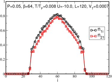
Figure 8: (color online). Density profiles of the two species for the low temperature and low polarization case. Very narrow fully paired regions are seen at the edges of the cloud. $N_{1}=39$ and $N_{2}=35$.

In Fig. 8 we show the density profiles at very low temperature, $T/T_{F}=0.008$, for a system at very small polarization, $P=0.05$, corresponding to the open (red) squares in Fig. 7. The central region of the system is clearly partially polarized: the profiles do not overlap. This partial polarization, i.e. population imbalance, causes FFLO pairing to take place as is evidenced by the pair momentum distribution in Fig. 7. However, in a very narrow interval at the edges of the system, the density profiles match very closely and the system is fully paired DrummondfiniteT ; hulet . This fully paired region was studied in the continuum casula using Path Integral Monte Carlo (PIMC) simulations. It was shown in Ref. casula that at a polarization $P=0.04$, the fully paired region exists for $T<0.025T_{F}$ and $T<0.035T_{F}$ for the two strong couplings studied (the first value corresponds to the smaller coupling). The narrowness of this region on the lattice was studied at $T=0$ in Ref. Meisner ; tezuka10 .

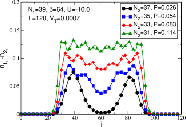
Figure 9: (color online). Density profile differences for different polarizations. The oscillations are standing waves showing the pair rich (minima) and pair depleted (maxima) regions in the confined system. $T/T_{F}=0.008$ for the balanced case with $N=78$ particles.

The difference in the density profiles, Fig. 9, of the two species shows regular oscillations indicating that the partially polarized region is not uniform. Such oscillations have been seen before feiguin07 ; tezuka07 ; batrouni08 . They correspond to the standing wave of length $\lambda=2\pi/k_{\rm peak}$, as can be easily verified from Figs. 7 and 9, and describe the length scale at which the system passes from pair-rich to pair-poor regions. This is a striking visual demonstration that the FFLO phase is not uniform.

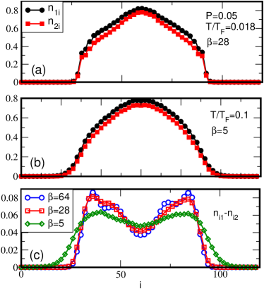
Figure 10: (color online). Trapped system at finite temperature and low polarization. (a) and (b) density profiles at $T/T_{F}=0.016$ and $T/T_{F}=0.1$ respectively. (c) density profile difference for different temperatures.

Next, we examine temperature effects on the system at low polarization. The system at $\beta=64$, Fig. 8, is now heated to $\beta=28$ ($T/T_{F}=0.016$) and $\beta=5$ ($T/T_{F}=0.1$) as shown in Fig. 10 (a) and (b) respectively. As the temperature increases, the clouds spread out and the profiles become more rounded. Figure 10 (c) shows what happens to the population differences as the temperature rises. As $T$ increases, the population difference vanishes in the wings more gradually than at the lower temperatures. In addition, the oscillations which indicate the presence of FFLO get smoothed out substantially at $\beta=28$ and have essentially disappeared for $\beta=5$. This is confirmed by the behaviour of the pair momentum distribution, displayed in Fig. 11, which shows the FFLO peak disappearing as $T$ is increased to $T=0.016T_{F}$. This value is smaller than, but consistent with, the phase diagram in Ref. DrummondfiniteT (Fig. 1) which shows that at $P=0.05$ the FFLO phase disappears for $T>0.05T_{F}$. Our value is also consistent with that found in Ref. casula . This illustrates the fragility of the fully paired paired wings and the FFLO phase at low polarization.

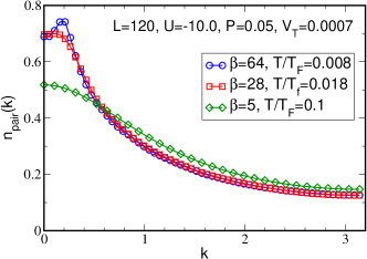
Figure 11: (color online). Pair momentum distribution of the system at P=0.05 (Fig. 10) and increasing temperature. The FFLO peak disappears at $T/T_{F}=0.016$.

IV.2 High polarization

In section III, we calculated the phase diagram of the uniform system and showed that the FFLO phase persists to higher temperatures for larger polarization. We now demonstrate the same effect in the trapped system.

Figure 12 shows the density profiles in the system with $P=0.56$ at $\beta=64$ ($T/T_{F}=0.01$). It is clear at this large $P$ that the central region is partially polarized and the wings are fully polarized, populated only by the majority species as was also observed in feiguin07 . The population difference in the central region of the system in Fig. 12 is almost constant but with oscillations, $\lambda=2\pi/k_{\rm peak}$, due to the presence of FFLO pairing as shown clearly by the pair momentum distribution in Fig. 13 (c).

Figure 12: (color online). Trapped system at low temperature and high polarization. $N_{1}=39,N_{2}=11,L=120$, $U/t=-10$, $V_{t}=0.0007$. $T_{F}$ is calculated for the total balanced population of $N=50$. Large fully polarized regions are seen at the boundaries of the system.

As the temperature is increased, this shell structure, i.e. partially polarized core and fully polarized wings, persists, as can be seen in Fig. 13 (a) and (b). However, we observe that the partially polarized core expands in size and the fully polarized population in the wings decreases. We also see that the FFLO phase at this large polarization is stabilized significantly compared with the $P=0.05$ case (Fig. 11). For $P=0.56$, the FFLO peak persists, albeit weakly, up to $T/T_{F}=0.11$, vanishing completely at $T/T_{F}=0.25$. This result is encouraging for the experiments hulet which can be done at high polarization and $T/T_{F}\approx 0.1$. However, at this temperature, the FFLO peak is not very pronounced and might still be difficult to observe experimentally.

We note that, as in the case of the uniform system, the FFLO phase disappears at a temperature which is much lower than the contact potential energy. In the case above, the FFLO phase disappears at $\beta t\approx 3$ while the contact interactions is $U=-10t$. The approximate condition to break the pairs is $\beta U\approx 1$; we see that $\beta t=3$ is not a high enough temperature to break the pairs. Therefore, as $T$ is increased, the FFLO phase is replaced by the PPP discussed in the previous section and not by the normal state composed of the two unpaired spin populations. Our QMC result is in disagreement with mean field predictions that as $T$ is increased for high polarization, the system passes directly from the FFLO phase to the normal state DrummondfiniteT .

As in the uniform case, the question arises as to whether one can stabilize the FFLO phase at higher temperature simply by increasing the attractive interactcion. The answer is the same as in the uniform case: As the attractive interaction is increased, the FFLO peak first increases in height but then saturates and starts to decrease. In addition, as $|U|$ is increased, the partially polarized core region shrinks and the polarization in that zone increases. This has the effect of shifting the FFLO peak to larger values of $k$. For the fillings we conisdered here, the value of the interactions we took, $U=-10t$, appears to be near optimal.

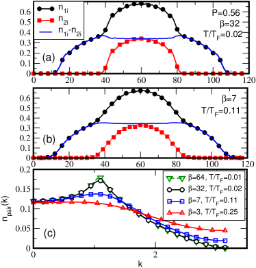
Figure 13: (color online). Same trapped system as in Fig. 12 at higher temperature. $P=0.56,L=120$, $U/t=-10$, $V_{t}=0.0007t$, $N_{1}=39$, $N_{2}=11$. (a) and (b) show the density profiles and differences for two temperature. (c) Pair momentum distribution.

V Conclusions

In this paper, we used three QMC algorithms (DQMC, canonical SGF and grand canonical SGF) to study the behaviour of one-dimensional imbalanced fermion systems with attractive interactions governed by the Hubbard Hamiltonian. We explored both the uniform and the confined cases.

In the uniform situation, we mapped the phase diagram in the polarization-temperature plane at two values of the total density (half filling and quarter filling) at the same interaction strength $U=-3.5t$. Both cases show the same general features: (1) The FFLO phase is very robust in the ground state and exists for a very wide range of polarizations; (2) at small polarization, the FFLO phase is very sensitive to temperature increase; (3) the FFLO phase persists to higher temperature when the polarization is larger and (4) the temperature at which the FFLO phase disappears is not high enough to break up the pairs leading to a spatially uniform polarized paired phase.

In the confined case, we performed our simulations for system parameters comparable to those in the experiment of Ref. hulet . We found the stability features of FFLO in the confined phase to be similar to those in the uniform case. At low polarization, the FFLO phase is destroyed even for a temperature as low as $T/T_{F}=0.016$. However, and this is significant for experimental efforts to detect FFLO in the confined system, we found that at large polarization, the FFLO phase persists at $T/T_{F}>0.11$ a temperature higher than that of the experiment, which has $T/T_{F}\approx 0.1$. Finally, the temperature at which the FFLO phase is destroyed is not high enough to break the pairs in disagreement with mean field results DrummondfiniteT .

- (1) J.E. Golub, K. Kash, J.P. Harbison, and L.T. Florez, Phys. Rev. B41, 8564 (1990).
- (2) J. Bardeen, L.N. Cooper and J.R. Schrieffer, Phys. Rev. 108, 1175 (1957).
- (3) V.L. Ginzburg and D.A. Kirzhnits, Soviet Phys. JETP 20, 1346 (1965); Nature 220, 148 (1968).
- (4) L. N. Cooper, Phys. Rev. 104, 1189 (1956).
- (5) P. Fulde and A. Ferrell, Phys. Rev. 135, A550 (1964).
- (6) A. Larkin and Y.N. Ovchinnikov, Zh. Eksp. Teor. Fiz. 47, 1136 (1964) [Sov. Phys. JETP 20, 762 (1965)].
- (7) G. Sarma, Phys. Chem. Solids 24, 1029 (1963); S. Takada and T. Izuyama, Prog. Theor. Phys. 41, 635 (1969).
- (8) H.A. Radovan, N.A. Fortune, T.P. Murphy, S.T. Hannahs, E.C. Palm, S.W. Tozer and D. Hall, Nature 425, 51 (2003).
- (9) R. Casalbuoni and G. Nardulli, Rev. Mod. Phys 76, 263 (2004).
- (10) M.W. Zwierlein, A. Schirotzek, C.H. Schunck and W. Ketterle, Science 311, 492 (2006); M.W. Zwierlein, C.H. Schunck, A. Schirotzek and W. Ketterle, Nature 422, 54 (2006); Y. Shin, M.W. Zwierlein, C.H. Schunck, A. Schirotzek and W. Ketterle, Phys. Rev. Lett. 97, 030401 (2006); Y. Shin, C.H. Schunck, A. Schirotzek and W. Ketterle, Nature 451, 689 (2008).
- (11) G.B. Partridge, W. Li, R.I. Kamar, Y. Liao and R.G. Hulet, Science 311, 503 (2006); G.B. Partridge, W. Li, Y. Liao, R.G. Hulet, M. Haque and H.T.C. Stoof, Phys. Rev. Lett. 97, 190407 (2006).
- (12) Y. Liao, A.S.C. Rittner, T. Paprotta, W. Li, G.B. Partridge, R.G. Hulet, S.K. Baur and E.J. Mueller arXiv:0912.0092v1 [physics.atom-ph].
- (13) P. Castorina, M. Grasso, M. Oertel, M. Urban and D. Zappalà , Phys. Rev. A72, 025601 (2005).
- (14) D.E. Sheehy and L. Radzihovsky, Phys. Rev. Lett. 96, 060401 (2006).
- (15) J. Kinnunen, L.M. Jensen and P. Törmä, Phys. Rev. Lett. 96, 110403 (2006).
- (16) K. Machida, T. Mizushima and M. Ichioka, Phys. Rev. Lett. 97, 120407 (2006).
- (17) K.B. Gubbels, M.W.J. Romans and H.T.C. Stoof, Phys. Rev. Lett. 97, 210402 (2006).
- (18) M.M. Parish, F.M. Marchetti, A. Lamacraft and B.D. Simons, Nature Phys. 3, 124 (2007).
- (19) H. Hu, X.-J. Liu and P.T. Drummond, Phys. Rev. Lett. 98, 070403 (2007).
- (20) Y. He, C.-C. Chien, Q. Chen and K. Levin, Phys. Rev. A75, 021602(R) (2007).
- (21) E. Gubankova, E. G. Mishchenko, and F. Wilczek, Phys. Rev. Lett. 94, 110402 (2005).
- (22) T. Koponen, J.-P. Martikainen, J. Kinnunen and P. Törmä, New J. Phys. 8, 179 (2006).
- (23) X.-J. Liu, H. Hu, P.D. Drummond, Phys. Rev. A76, 043605 (2007).
- (24) D.T. Son and M.A. Stephanov, Phys. Rev. A74, 013614 (2006).
- (25) G. Orso, Phys. Rev. Lett. 98, 070402 (2007).
- (26) G.G. Batrouni, M.H. Huntley, V.G. Rousseau and R.T. Scalettar, Phys. Rev. Lett. 100, 116405 (2008).
- (27) M. Casula, D.M. Ceperley, and E.J. Mueller, Phys. Rev. A78, 033607 (2008).
- (28) A. Feiguin and F. Heidrich-Meisner, Phys. Rev. B76, 220508(R) (2007).
- (29) A. Lüscher, R.M. Noack, and A.M. Läuchli, Phys. Rev. A78, 013637 (2008).
- (30) M. Rizzi, M. Pollini, M. Cazalilla, M. Bakhtiari, M. Tosi and R. Fazio, Phys. Rev. B77, 245105 (2008).
- (31) M. Tezuka and M. Ueda, Phys. Rev. Lett. 100, 110403 (2008).
- (32) X. Liu, H. Hu, P.D. Drummond, Phys. Rev. A78, 023601 (2008).
- (33) P. Kakashvili and C.J. Bolech, Phys. Rev. A79, 041603(R) (2009).
- (34) T.K. Koponen, T.Paananen, J.-P. Martikainen, M.R.Bakhtiari and P. Törmä, New J. Phys. 10 045014 (2008).
- (35) W. V. Liu, F. Wilczek, Phys. Rev. Lett. 90, 047002 (2003).
- (36) E. Gubankova, W. V. Liu, F. Wilczek, Phys. Rev. Lett. 91, 032001 (2003).
- (37) G. G. Batrouni, M. J. Wolak, F. Hébert, V. G. Rousseau, Europhysics Letters 86, 47006 (2009).
- (38) R. Blankenbecler, D.J. Scalapino, and R.L. Sugar, Phys. Rev. D24, 2278 (1981); S.R. White, D.J. Scalapino, R.L. Sugar, E.Y. Loh, J.E. Gubernatis, and R.T. Scalettar, Phys. Rev. B40, 506 (1989).
- (39) V.G. Rousseau, Phys. Rev. E 77, 056705(2008).
- (40) V.G. Rousseau, Phys. Rev. E 78, 056707(2008).
- (41) Y.L. Loh and N. Trivedi, arXiv:0907.0679v1 [cond-mat.quant-gas].
- (42) F. Heidrich-Meisner, G. Orso, A.E. Feiguin arXiv:1001.4720v1 [cond-mat.quant-gas]
- (43) M. Tezuka and M. Ueda, arXiv:1002.1433.