Plasma Magnetosphere of Rotating Magnetized Neutron Star in the Braneworld

Abstract

Plasma magnetosphere surrounding rotating magnetized neutron star in the braneworld has been studied. For the simplicity of calculations Goldreich-Julian charge density is analyzed for the aligned neutron star with zero inclination between magnetic field and rotation axis. From the system of Maxwell equations in spacetime of slowly rotating star in braneworld, second-order differential equation for electrostatic potential is derived. Analytical solution of this equation indicates the general relativistic modification of an accelerating electric field and charge density along the open field lines by brane tension. The implication of this effect to the magnetospheric energy loss problem is underlined. It was found that for initially zero potential and field on the surface of a neutron star, the amplitude of the plasma mode created by Goldreich-Julian charge density will increase in the presence of the negative brane charge. Finally we derive the equations of motion of test particles in magnetosphere of slowly rotating star in the braneworld. Then we analyze particle motion in the polar cap and show that brane tension can significantly change conditions for particle acceleration in the polar cap region of the neutron star.

Received (Day Month Year)Revised (Day Month Year)

1 Introduction

Amazing idea about hidden extra-dimensions of our Universe attracted scientific interest almost from the beginning of 20th century. First attempts of building multidimensional models were proposed by Kaluza in order to unify electromagnetism with gravity already in 1920s [18]. Then these ideas found reflection in elegant string theory which is the subject of extensive research in modern physics and promise to throw light upon many puzzles of nature. One of the most recent theories including extra dimensions is the braneworld picture of the Universe.

The braneworld model was first proposed by [37] assuming that our four-dimensional space-time is just a slice of five-dimensional bulk. According to this model only gravity is the force which can freely propagate between our space-time and bulk while other fields are confined to four-dimensional Universe. In this view it is noteworthy to look for effects of fifth dimension on our world in frame of theory of gravity i.e. general relativity. Possible tools for proving braneworld model should be found from astrophysical objects, namely, compact objects, for which effects of general relativity are especially strong. For example, investigations of cosmological and astrophysical implications of the braneworld theories may be found in [24], [10], [22], [17], [14], [21], [26]. Review of braneworld models is given e.g. in [25]. In the context of the braneworld, a method to find consistent solutions to Einstein’s field equations in the interior of a spherically symmetric, static and non uniform stellar distribution with Weyl stresses is developed in the work of [34].

For astrophysical interests, static and spherically symmetric exterior vacuum solutions of the braneworld models were initially proposed by Dadhich et al. [11] which have the mathematical form of the Reissner-Nordström solution, in which a tidal Weyl parameter $Q^{\ast}$ plays the role of the electric charge squared of the general relativistic solution.

Observational possibilities of testing the braneworld black hole models at an astrophysical scale have been intensively discussed in the literature during the last several years, for example, through the gravitational lensing, the motion of test particles, and the classical tests of general relativity (perihelion precession, deflection of light, and the radar echo delay) in the Solar System (see [9]). In paper [36] the energy flux, the emission spectrum, and accretion efficiency from the accretion disks around several classes of static and rotating braneworld black holes have been obtained. The complete set of analytical solutions of the geodesic equation of massive test particles in higher dimensional spacetimes which can be applied to braneworld models is provided in the recent paper [16]. The relativistic quantum interference effects in the spacetime of slowly rotating object in braneworld and phase shift effect of interfering particle in neutron interferometer have been studied in the recent paper [27]. The influence of the tidal charge onto profiled spectral lines generated by radiating tori orbiting in the vicinity of a rotating black hole has been studied in paper [43]. Authors showed that with lowering the negative tidal charge of the black hole, the profiled line becomes flatter and wider, keeping their standard character with flux stronger at the blue edge of the profiled line. The role of the tidal charge in the orbital resonance model of quasiperiodic oscillations in black hole systems has been investigated in paper [45]. The influence of the tidal charge parameter of the braneworld models on some optical phenomena in rotating black hole spacetimes has been extensively studied in paper [44].

A braneworld corrections to the charged rotating black holes and to the perturbations in the electromagnetic potential around black holes are studied, for example, in [3, 1]. The motion of test particles near black holes immersed in an asymptotically uniform magnetic field and some gravity surrounding structure, which provides the magnetic field has been intensively studied in paper [19]. The author has calculated the binding energy for spinning particles on circular orbits. The bound states of the massive scalar field around a rotating black hole immersed in the asymptotically uniform magnetic field are considered in paper [20]. The uniform magnetic field in the background of a five dimensional black hole has been extensively studied in [4]. In particular, authors presented exact expressions for two forms of an electromagnetic tensor and the electrostatic potential difference between the event horizon of a five dimensional black hole and the infinity.

Among astrophysical objects which can be useful in investigating high-dimensional models particular place belongs to radio pulsars. Radio pulsars are rotating highly magnetized neutron stars, producing radio emission above the small area of its surface called polar cap. [15] proved that such a rotating highly magnetized star cannot be surrounded by vacuum due to generation of strong electric field pulling out charged particles from the surface of the star. They proposed first model of the pulsar magnetosphere containing two distinct regions: the region of closed magnetic field lines, where plasma corotates with the star as a solid body, and the region of open magnetic field lines, where radial electric field is not completely screened with plasma particles and plasma may leave the neutron star along magnetic field lines. Radio emission is generated due to continuous cascade generation of electron-positron pairs in the magnetosphere above the polar cap. Thorough research on structure and physical processes in pulsar magnetosphere can be found in works of [15], [47], [28], [42], [5], [31]. Although a self-consistent pulsar magnetosphere theory is yet to be developed, the analysis of plasma modes in the pulsar magnetosphere based on the above-mentioned papers provides firm ground for the construction of such a model.

It was shown by a number of authors that effects of general relativity play very important role in physics of pulsars. General relativistic effects on the vacuum electromagnetic fields around slowly rotating magnetized neutron stars were investigated by [39], [40]. The effect of general relativistic frame dragging effect in the plasma magnetosphere was investigated in [7], [33], [31], [29], [8] and proved to be crucial for the conditions of particle acceleration in the magnetosphere and, therefore, for generation of radio emission. From the above mentioned papers it is seen that the general relativistic effects in the magnetosphere of pulsars are not negligible and should be carefully considered.

Our preceding paper [2] was devoted to the stellar magnetic field configurations of relativistic stars in dependence on brane tension and the present research extends it to the case of rotating relativistic star. Here we will consider rotating spherically symmetric star in the braneworld endowed with strong magnetic fields. We assume that the star has dipolar magnetic field and the field energy is not strong enough to affect the spacetime geometry, so we consider the effects of the gravitational field of the star in the braneworld on the magnetic and electric field structure without feedback. That is our present research is devoted to the strong gravity effects in pulsar magnetosphere in frame of the braneworld model. We use results of the work of [33] initiated the detailed general relativistic derivation of magnetospheric electromagnetic fields around rotating magnetized neutron star. In section 2 we analyse Goldreich-Julian charge density for the case of slowly rotating neutron star in the braneworld and get solution for Poisson equation in this case. In sections 3 and 4 we have studied plasma modes along the open field lines of the rotating magnetized neutron star in the braneworld. Section 5 is devoted to the charged particle acceleration in the polar cap of the rotating star in the braneworld. Section 6 summarizes the obtained results.

Throughout the paper we use a space-like signature $(-,+,+,+)$ and a system of units in which $G=1=c$. Latin indices run $1,2,3$ and Greek ones from $0$ to $3$.

2 Plasma Magnetosphere of Slowly Rotating Magnetized Star in the Braneworld

In a pioneering work, [15] have shown that a strongly magnetized, highly conducting neutron star, rotating about the magnetic axis, would spontaneously build up a charged magnetosphere. Strong magnetic field of the star together with rotation create strong radial electric field component $E_{\parallel}\sim 10^{10}-10^{12}\ V\ cm^{-1}$ on the surface of the star. Such a strong field make charged particles escape from the surface of the star and form plasma magnetosphere around the star. Plasma charges, in turn, partially screen radial electric field and ${\bf{E}}\times{\bf{B}}$ drift sets them into corotation with the star. The magnetosphere charge density which would be necessary for complete screening of $E_{\parallel}$ is called the corotation charge density or the Goldreich-Julian density. In the region of the polar cup magnetospheric charge does not screen $E_{\parallel}$ completely, what results in continuous flow of accelerated charged particles from the surface of the polar cap responsible for later generation of radioemission from the region.

In general, Goldreich-Julian charge density $\rho_{GJ}$ can be found through the formula

$$\rho_{GJ}=-\frac{1}{4\pi}{\mathbf{\nabla}}(N{\bf g}\times{\bf B})\ ,$$ (1)

where $g_{i}=-g_{0i}/g_{00}$ can be found with the help of the metric of given space-time, $N$ is the lapse function.

The metric, describing external space-time for the rotating star in the braneworld, has the following form in spherical coordinates

$$ds^{2}=-A^{2}dt^{2}+H^{2}dr^{2}+r^{2}d\theta^{2}+r^{2}\sin^{2}\theta d\phi^{2}$$

$$\qquad\quad-2\tilde{\omega}(r)r^{2}\sin^{2}\theta dtd\phi\ .$$ (2)

This metric is derived from the general solution for the rotating star on the branes [36] under the assumption that specific angular momentum $a=J/M$ is small. In the equation (2)

$$A^{2}(r)\equiv\left(1-\frac{2M}{r}+\frac{Q^{\ast}}{r^{2}}\right)=H^{-2}(r),\ \ \ \ \ \ \ \ r>R$$ (3)

and $\tilde{\omega}(r)=\omega(1-Q^{\ast}/2rM)$, $Q^{\ast}$ is the bulk tidal charge, $M$ is the mass of the star, $\omega=2Ma/r^{3}$ is the angular velocity of the dragging of inertial frames.

In frames of metric (2) one can obtain the following equations for the vector ${\bf g}$

$${\bf g}=\frac{1}{A^{2}}\left[{\mathbf{\Omega}}-\left(1-\frac{Q^{\ast}}{2rM}\right){\mathbf{\omega}}\right]\times{\bf r}$$ (4)

and Goldreich-Julian charge density

$$\rho_{GJ}=-\frac{1}{4\pi}{\mathbf{\nabla}}\left\{\frac{1}{A}\left[1-\left(1-\frac{Q^{\ast}}{2\eta RM}\right)\frac{\kappa}{\eta^{3}}\right]{\bf u}\times{\bf B}\right\}\ ,$$ (5)

where ${\bf u}={\mathbf{\Omega}}\times{\bf r}$, $\eta=r/R$ is the dimensionless radial coordinate, parameter $\kappa\equiv\varepsilon\beta$, $\varepsilon=2M/R$ is the compactness parameter, and $\beta=I/I_{0}$ is the stellar moment of inertia in the units of $I_{0}=MR^{2}$.

In the work [33] the expressions for the components of dipolar magnetic field ${\bf B}$ in the vicinity of the slowly rotating neutron star are presented. In these calculations the metric of space-time was assumed to have the following form:

$$ds^{2}=-N^{2}dt^{2}+N^{-2}dr^{2}+r^{2}d\theta^{2}+r^{2}\sin^{2}\theta d\phi^{2}$$

$$\qquad\quad-2\omega r^{2}\sin^{2}\theta dtd\phi\ ,$$ (6)

where $N^{2}\equiv(1-2M/r)$. Being measured by zero angular momentum observer (ZAMO) with 4-velocity $u_{\alpha}=\left\{-N,0,0,0\right\}$ components of dipolar magnetic field have the form

$$B^{\hat{r}}=B_{0}\frac{f(\eta)}{f(1)}\eta^{-3}\cos\theta\ ,$$ (7)

$$B^{\hat{\theta}}=\frac{1}{2}B_{0}N\left[-2\frac{f(\eta)}{f(1)}+\frac{3}{(1-\varepsilon/\eta)f(1)}\right]\eta^{-3}\sin\theta\ ,$$

with

$$f(\eta)=-3\left(\frac{\eta}{\varepsilon}\right)^{3}\left[\ln\left(1-\frac{\varepsilon}{\eta}\right)+\frac{\varepsilon}{\eta}\left(1+\frac{\varepsilon}{2\eta}\right)\right]\ ,$$ (8)

where $B_{0}\equiv 2\mu/R^{3}$ is the Newtonian value of the magnetic field at the pole of star, hats label the orthonormal components and $\mu$ is the magnetic moment. In the spacetime of the slowly rotating neutron star in the braneworld Maxwell equations for the magnetic form have a little more complicated form and avoid exact analytical solution yet. Nevertheless, one may expect that corrections to the magnetic field due to tidal charge $Q^{\ast}$ will be small in comparison with main expression. In our research for the simplicity of the calculations we are going to neglect these corrections and use equation (7) for the magnetic field of the star.

Inserting equation (7) into equation (5) we get the following final form for the Goldreich-Julian charge density

$$\rho_{GJ}=-\frac{\Omega B_{0}}{2\pi c}\frac{1}{A\eta^{3}}\frac{f(\eta)}{f(1)}\left\{1-\left(1-\frac{Q^{\ast}}{2\eta RM}\right)\frac{\kappa}{\eta^{3}}\right\}\ .$$ (9)

In the papers [32], [33] the expression for the polar angle $\Theta$ of the last open magnetic line as a function of $\eta$ can be found

$$\Theta\cong\sin^{-1}\left\{\left[\eta\frac{f(1)}{f(\eta)}\right]^{1/2}\sin\Theta_{0}\right\}\ ,$$

$$\Theta_{0}=\sin^{-1}\left(\frac{R}{R_{LC}f(1)}\right)^{1/2}\ ,$$ (10)

where $\Theta_{0}$ is the magnetic colatitude of the last open magnetic line at the stellar surface, $R_{LC}=c/\Omega$ is the light-cylinder radius.

Assuming the magnetic field of a neutron star to be stationary in the corotating frame, from the system of Maxwell equations the following Poisson equation for the scalar potential $\Phi$ can be derived (look [33])

$${\mathbf{\nabla}}\cdot\left(\frac{1}{A}{\mathbf{\nabla}}\Phi\right)=-4\pi(\rho-\rho_{GJ})\ ,$$ (11)

where $\rho-\rho_{GJ}$ is the effective space charge density being responsible for production of unscreened parallel electric field.

Choosing the following form for the charge density $\rho$ in the vicinity of the surface of the neutron star

$$\rho=\frac{\Omega B_{0}}{2\pi c}\frac{1}{A\eta^{3}}\frac{f(\eta)}{f(1)}C(\xi)\ ,$$ (12)

where $\xi=\theta/\Theta$ is the dimensionless angular variable, $C(\xi)$ is an unknown angular dependent function to be defined from the boundary conditions, and inserting equations (12) and (9) into the Poisson equation (11) one can obtain under the approximation of small angles $\theta$ the following differential equation

$$R^{-2}\bigg{\{}A\frac{1}{\eta^{2}}\frac{\partial}{\partial\eta}\left(\eta^{2}\frac{\partial}{\partial\eta}\right)$$ (13)

$$\qquad\qquad+\frac{1}{A\eta^{2}\theta}\left[\frac{\partial}{\partial\theta}\left(\theta\frac{\partial}{\partial\theta}\right)+\frac{1}{\theta}\frac{\partial^{2}}{\partial\phi^{2}}\right]\bigg{\}}\Phi=$$

$$-4\pi\frac{\Omega B_{0}}{2\pi c}\frac{1}{A\eta^{3}}\frac{f(\eta)}{f(1)}\left\{1-\left(1-\frac{Q^{\ast}}{2\eta RM}\right)\frac{\kappa}{\eta^{3}}+C(\xi)\right\}.$$

Our further discourses are based on the extension of work [33]. Using dimensionless function $F=\eta\Phi/\Phi_{0}$, where $\Phi_{0}=\Omega B_{0}R^{2}$ and variables $\eta$ and $\xi$, one can rewrite the equation (13) as

$$\left[\frac{d^{2}}{d\eta^{2}}+\Lambda^{2}(\eta)\frac{1}{\xi}\frac{\partial}{\partial\xi}\left(\xi\frac{\partial}{\partial\xi}\right)\right]F=-\frac{2}{\eta^{2}-\varepsilon\eta+\tilde{Q^{\ast}}}$$

$$\frac{f(\eta)}{f(1)}\left[1-\left(1-\frac{Q^{\ast}}{2\eta RM}\right)\frac{\kappa}{\eta^{3}}+C(\xi)\right]\ ,$$ (14)

where $\Lambda(\eta)=[\eta\Theta(\eta)(1-\varepsilon/\eta+\tilde{Q^{\ast}}/\eta^{2})^{1/2}]^{-1}$ and $\tilde{Q^{\ast}}=Q^{\ast}/R^{2}$.

One can apply Fourier-Bessel transformation

$$F(\eta,\xi)=\sum_{i=1}^{\infty}F_{i}(\eta)J_{0}(k_{i}\xi)\ ,$$

$$F_{i}(\eta)=\frac{2}{[J_{1}(k_{i})]^{2}}\int^{1}_{0}\xi F(\eta,\xi)J_{0}(k_{i}\xi)d\xi\ ,$$ (15)

with the relation

$$\sum_{i=1}^{\infty}\frac{2}{k_{i}J_{1}(k_{i})}J_{0}(k_{i}\xi)=1\ ,$$ (16)

to obtain equation (14) in the form

$$\left(\frac{d^{2}}{d\eta^{2}}-\gamma^{2}_{i}(\eta)\right)F_{i}=-\frac{2}{\eta^{2}-\varepsilon\eta+\tilde{Q^{\ast}}}\frac{f(\eta)}{f(1)}$$

$$\left[\frac{2}{k_{i}J_{1}(k_{i})}\left\{1-\left(1-\frac{Q^{\ast}}{2\eta RM}\right)\frac{\kappa}{\eta^{3}}\right\}+C_{i}\right],$$ (17)

where $\gamma^{2}_{i}=k^{2}_{i}\Lambda^{2}$, $k_{i}$ are positive zeros of the functions $J_{0}$.

Considering a region near the surface of the star, where $z=\eta-1\ll 1$, and using following boundary conditions (that is the conditions of equipotentiality of the stellar surface and zero steady state electric field at $r=R$)

$$F_{i}|_{z=0}=0\ ,\ \frac{\partial F_{i}}{\partial z}|_{z=0}=0\$$ (18)

one can find the expression for the scalar potential $\Phi$ near the surface of the star and corresponding to this potential component of the electric field $E_{\|}$, being parallel to the magnetic field (see the discourses of [33] work):

$$\Phi=\frac{12\Phi_{0}}{\eta}\sqrt{1-\varepsilon+\tilde{Q^{\ast}}}\kappa\left(1-\frac{2Q^{\ast}}{3MR}\right)\Theta^{3}_{0}$$

$$\sum^{\infty}_{i=1}\Bigg{[}\exp\bigg{\{}\frac{k_{i}(1-\eta)}{\Theta_{0}\sqrt{1-\varepsilon+\tilde{Q^{\ast}}}}\bigg{\}}-1$$

$$\qquad\qquad+\frac{k_{i}(\eta-1)}{\Theta_{0}\sqrt{1-\varepsilon+\tilde{Q^{\ast}}}}\Bigg{]}\frac{J_{0}(k_{i}\xi)}{k_{i}^{4}J_{1}(k_{i})}\ ,$$ (19)

$$E_{\|}=-\frac{12\Phi_{0}}{R}\kappa\left(1-\frac{2Q^{\ast}}{3MR}\right)\Theta^{2}_{0}$$

$$\sum^{\infty}_{i=1}\left[1-\exp\left\{\frac{k_{i}(1-\eta)}{\Theta_{0}\sqrt{1-\varepsilon+\tilde{Q^{\ast}}}}\right\}\right]\frac{J_{0}(k_{i}\xi)}{k_{i}^{3}J_{1}(k_{i})}\ .$$ (20)

Considering now the region $\Theta_{0}\ll\eta-1\ll R_{LC}/R$, where $|d^{2}F_{i}/d\eta^{2}|\ll\gamma^{2}_{i}(\eta)|F_{i}|$ one can see that equation (17) becomes

$$-\gamma^{2}_{i}(\eta)F_{i}=-\frac{2}{\eta^{2}-\varepsilon\eta+\tilde{Q^{\ast}}}\frac{f(\eta)}{f(1)}$$

$$\left[\frac{2}{k_{i}J_{1}(k_{i})}\left\{1-\left(1-\frac{Q^{\ast}}{2\eta RM}\right)\frac{\kappa}{\eta^{3}}\right\}+C_{i}\right]\ ,$$ (21)

from which it immediately follows

$$F_{i}=4\kappa\theta^{2}(\eta)\frac{f(\eta)}{f(1)}\bigg{[}1-\frac{Q^{\ast}}{2RM}-\left(1-\frac{Q^{\ast}}{2\eta RM}\right)\frac{1}{\eta^{3}}$$

$$-\frac{3}{\gamma_{i}(1)}\left(1-\frac{2Q^{\ast}}{3MR}\right)\bigg{]}\frac{1}{k_{i}^{3}J_{1}(k_{i})}\simeq$$

$$4\kappa\Theta_{0}^{2}\eta\left[1-\frac{Q^{\ast}}{2RM}-\left(1-\frac{Q^{\ast}}{2\eta RM}\right)\frac{1}{\eta^{3}}\right]\frac{1}{k_{i}^{3}J_{1}(k_{i})}.$$ (22)

Using this expression for $F_{i}$ one can obtain the scalar potential in the region at distances greater than the polar cap size as

$$\Phi=\frac{\Phi_{0}}{\eta}F=2\Phi_{0}\Theta^{2}_{0}\kappa$$

$$\left[1-\frac{Q^{\ast}}{2RM}-\left(1-\frac{Q^{\ast}}{2\eta RM}\right)\frac{1}{\eta^{3}}\right]\sum_{i}\frac{2J_{0}(k_{i}\xi)}{k^{3}_{i}J_{1}(k_{i})}$$

$$=\frac{\Phi_{0}\Theta_{0}^{2}\kappa}{2}\left[1-\frac{Q^{\ast}}{2RM}-\left(1-\frac{Q^{\ast}}{2\eta RM}\right)\frac{1}{\eta^{3}}\right](1-\xi^{2})$$

$$=\frac{\Omega R^{2}B_{0}\Theta_{0}^{2}\kappa}{2}\left[1-\frac{1}{\eta^{3}}-\frac{Q^{\ast}}{2MR}\left(1-\frac{1}{\eta^{4}}\right)\right](1-\xi^{2})\ .$$

Corresponding to this potential component of electric field $E_{\|}$ will look like

$$E_{\|}=-\frac{1}{R}\frac{\partial\Phi}{\partial\eta}|_{\xi=constant}=$$

$$\qquad-\frac{E_{vac}\Theta^{2}_{0}\kappa}{2}\left(\frac{3}{\eta^{4}}-\frac{2Q^{\ast}}{MR}\frac{1}{\eta^{5}}\right)(1-\xi^{2})\ ,$$ (24)

where $E_{vac}\equiv(\Omega R/c)B_{0}$ is the characteristic Newtonian value of the electric field generated near the surface of a neutron star rotating in vacuum [12].

Using expression from the work of [31] for the total power carried away by relativistically moving particles

$$L_{p}=2(-c\int\rho\Phi\ dS)\ .$$ (25)

one can obtain for the maximum of $L_{p}$

$$(L_{p})_{max}=$$

$$\frac{3}{2}\kappa\left(1-\frac{Q^{\ast}}{2MR}\right)\left[1-\kappa\left(1-\frac{Q^{\ast}}{2MR}\right)\right]\dot{E}_{rot}\ ,$$ (26)

where

$$\dot{E}_{rot}\equiv\frac{1}{6}\frac{\Omega^{4}B_{0}^{2}R^{6}}{c^{3}f^{2}(1)}=\frac{1}{f^{2}(1)}(\dot{E}_{rot})_{Newt}\$$ (27)

and $(\dot{E}_{rot})_{Newt}$ is the standard Newtonian expression for the magneto-dipole losses in flat space-time approximation.

One can see that obtained equation (26) differs from corresponding equation from the work of [31] for the case of slowly rotating neutron star $(L_{p})_{max}=\frac{3}{2}\kappa(1-\kappa)\dot{E}_{rot}$ by replacing $\kappa$ with $\kappa(1-Q^{\ast}/2MR)$.

In terms of pulsar’s period $P$ and its time derivative $\dot{P}\equiv dP/dt$ equation (26) will look as

$$(P\dot{P})_{max}=\frac{3}{4}\kappa\left(1-\frac{Q^{\ast}}{2MR}\right)$$

$$\qquad\left[1-\kappa\left(1-\frac{Q^{\ast}}{2MR}\right)\right]\frac{I}{\tilde{I}}\frac{1}{f^{2}(1)}(P\dot{P})_{Newt}\ ,$$ (28)

where

$$(L_{p})_{max}=-\tilde{I}(\Omega\dot{\Omega})_{max}$$ (29)

and

$$(P\dot{P})_{Newt}\equiv\left(\frac{2\pi^{2}}{3c^{3}}\right)\frac{R^{6}B^{2}_{0}}{I}\ .$$ (30)

In equation (29) $\tilde{I}$ is the general relativistic moment of inertia of the star (see e.g. [41])

$$\tilde{I}\equiv\int d^{3}\mathbf{x}\sqrt{\gamma}e^{-\Phi(r)}\rho r^{2}\sin^{2}\theta\ ,$$ (31)

where $e^{-\Phi(r)}\equiv 1/\sqrt{-g_{00}}$, $\rho(r)$ is the total energy density, $\gamma$ is the determinant of the three metric and $d^{3}\mathbf{x}$ is the coordinate volume element.

Expression (28) could be used to investigate the rotational evolution of magnetized neutron stars with plasma magnetosphere. A detailed investigation of general relativistic effects for Schwarzschild stars in vacuum has already been performed by [35], who have paid special attention to the general relativistic corrections that need to be included for a correct modeling of the thermal evolution but also of the magnetic and rotational evolution. It should be remarked, however, that in their treatment [35] have taken into account the general relativistic amplification of magnetic field due to the curved background spacetime, but did not include the corrections due to the gravitational redshift. As a result, the general relativistic electromagnetic luminosity estimated by [35] is smaller than the one computed in paper [41] where all general relativistic effects are taken into account. The evolution of low-mass X-ray binaries hosting a neutron star and of millisecond binary radio pulsars using numerical simulations that take into account the detailed evolution of the companion star, of the binary system, and of the neutron star has been studied in the paper [23].

3 Linear Plasma Modes Along the Open Field Lines

The theory of cascade generation of electron-positron plasma at the polar cap region of a rotating plasma is developed by [42]. According to the theoretical model, because of the escape of charge particles along the open field lines, a polar potential gap is produced that continuously breaks down by forming an electron-positron pair on a timescale of a few microseconds. A photon of energy greater than $2mc^{2}$ produces an electron-positron pair. The electric field of the gap accelerates the positron out of the gap and accelerates the electron toward the stellar surface. The electron moves along a curved magnetic field line and radiates an energetic photon that goes on to produce a pair as it has a sufficient component of momentum perpendicular to the magnetic .eld. Recently, [48] explained the $e-e^{+}$ pair production from a Crab-like pulsar. Electrons and positrons are accelerated in opposite directions to extremely high energies. The Lorentz factor $\gamma$ of the ”primary” electron and positron is given by

$$e\mathbf{E}\cdot\mathbf{B}c\approx\frac{e^{2}}{c^{3}}\gamma^{4}\left(\frac{c^{2}}{r_{c}}\right)^{2},$$ (32)

where $r_{c}$ is the curvature radius of the local magnetic field lines and $\mathbf{E}\cdot\mathbf{B}$ is the pulsar magnetospheric electric field component along $\mathbf{B}$. For the Crab pulsar, the above equation gives $\gamma$ of the order of $10^{7}$. Curvature photons radiated by the primary electrons and positrons have energy $\approx h\gamma^{3}(c/r_{c})$. Each primary electron and positron would produce about $N_{\gamma}\approx(\gamma e^{2}/hc)\approx 10^{5}$ curvature photons. To sustain the primary current flow and account for the observed X-ray and $\gamma$-ray luminosity from the Crab pulsar, the needed primary particle flux is around $10^{33}s^{-1}$. This cascade of pair production, acceleration of electrons and positrons along curved field lines, curvature radiation, and pair production results in a ”spark” breakdown of the gap. Linear and nonlinear plasma modes near the slowly rotating neutron star has been studied in the work of [29]. Here we will generalize the obtained results into the case when the neutron star is considered in the braneworld.

Assuming a steady state thermodynamical equilibrium plasma state in the polar cap region, we study the linear plasma modes along the field lines. From the charge continuity equation

$$\frac{\partial\rho}{\partial t}+\left(\frac{\kappa}{r^{3}}-1\right)\Omega m\cdot\nabla\rho+\nabla\cdot(A\mathbf{j})=0\ ,$$ (33)

the equation of motion of the charged particle

$$\left[\frac{\partial}{\partial t}+\left(\frac{\kappa}{r^{3}}-1\right)\Omega\cdot\nabla+A\bf{v}\cdot\nabla\right]\mathbf{p}=-q\nabla\Phi\ ,$$ (34)

and the equation (11), one can easily derive the following linearized equations:

$$\nabla\left[\left(1-\frac{2M}{r}+\frac{Q^{*}}{r^{2}}\right)^{-1/2}\nabla\Phi\right]=-4\pi(\rho-\rho_{\rm GJ})\ ,$$ (35)

$$\frac{\partial\rho}{\partial t^{\prime}}+\nabla\frac{\partial}{\partial t^{\prime}}\left(1-\frac{2M}{r}+\frac{Q^{*}}{r^{2}}\right)^{1/2}\mathbf{j}_{\rm s}\ ,$$ (36)

$$\frac{\partial\mathbf{v}_{\rm s}}{\partial t^{\prime}}=-\frac{e_{s}}{m}\nabla\Phi\ ,$$ (37)

where $\partial/\partial t^{\prime}=\partial/\partial t+(\kappa/r^{3}-1)\Omega\cdot\nabla$ is the global time derivative along ZAMO trajectories, $\mathbf{j}_{\rm s}$ is the current density and $e_{\rm s}$ is the electric charge of the particle, Goldreich-Julian charge density $\rho_{\rm GJ}$ is defined by the equation (9).

From the system of equations (35)–(37) one can get the following equivalent equation:

$$\frac{\partial^{2}}{\partial t^{\prime 2}}\left\{\nabla\left[\left(1-\frac{2M}{r}+\frac{Q^{*}}{r^{2}}\right)^{-1/2}\nabla\Phi\right]\right\}+$$

$$\nabla\left[\omega_{p}^{2}\left(1-\frac{2M}{r}+\frac{Q^{*}}{r^{2}}\right)^{1/2}\nabla\Phi\right]=0\ ,$$ (38)

where $\omega_{p}^{2}=8\pi\rho e_{\rm s}/m$. Using the following notations

$$\mathbf{E}=-\left(1-\frac{2M}{r}+\frac{Q^{*}}{r^{2}}\right)^{-1/2}\nabla\Phi\ ,$$ (39)

$$\rho_{\rm GJ}=\frac{1}{4\pi}\nabla\mathbf{E}_{\rm c}\ ,$$ (40)

equation (38) can be rewritten as

$$\frac{\partial^{2}}{\partial t^{\prime 2}}\nabla\left(\mathbf{E}+\mathbf{E}_{\rm c}\right)+\nabla\omega_{\rm p}^{2}\left(1-\frac{2M}{r}+\frac{Q^{*}}{r^{2}}\right)\mathbf{E}=0\ .$$ (41)

If we take into account that $\mathbf{E}_{\rm c}=const$, then we have the following ordinary differential equation:

$$\frac{\partial^{2}\mathbf{E}}{\partial t^{\prime 2}}+\omega_{\rm p}^{2}\left(1-\frac{2M}{r}+\frac{Q^{*}}{r^{2}}\right)\mathbf{E}$$ (42)

which has solution of form

$$E=E_{0}\exp\left(i\omega_{p}\sqrt{1-\frac{2M}{r}+\frac{Q^{*}}{r^{2}}}\ t\right)=E_{0}\exp\left(i\omega t\right)\ .$$ (43)

$\omega=\omega_{p}\sqrt{1-{2M}/{r}+{Q^{*}}/{r^{2}}}$ can be thought as plasma frequency in general relativity, which is equivalent to the gravitational redshift of the oscillation. Figure 1 shows the radial dependence of the frequency $\omega$ for the different values of the brane parameter $Q^{*}$. The increase of the module of the brane parameter causes shift of the plasma modes to the red direction.

Figure 1: The radial dependence of the $\omega$ for the different values of the brane tension $Q^{*}$ .

The global time derivative along ZAMO trajectories is defined as:

$$\frac{\partial}{\partial t^{\prime}}=\frac{\partial}{\partial t}+\left(\frac{\kappa}{r^{3}}-1\right)\Omega\frac{\partial}{\partial\phi}\ ,$$ (44)

that is one may define

$${t^{\prime}}={t}+\frac{\phi}{\left({\kappa}/{r^{3}}-1\right)\Omega}\ ,$$ (45)

and hence the solution of linear plasma mode is

$$E=$$

$$E_{0}\exp\left\{i\omega_{p}\sqrt{1-\frac{2M}{r}+\frac{Q^{*}}{r^{2}}}\ \left[{t}+\frac{\phi}{\left({\kappa}/{r^{3}}-1\right)\Omega}\right]\right\}.$$ (46)

Now, introducing new dimensionless parameters as $\epsilon=E/E_{0}$, $\tau=\omega_{p}t$, $\chi=\omega_{p}/\Omega$, $\delta=\kappa/{8M^{3}}$, and $q=Q^{*}/{M^{2}}$ we get from equation (46):

$$\epsilon=\sin\left[\sqrt{1-\frac{2}{\eta}+\frac{q}{\eta^{2}}}\ \left(\tau+\frac{\chi}{{8\delta}/{\eta^{3}}-1}\phi\right)\right]\ .$$ (47)

Figure 2 shows the radial dependence of the dimensionless quantity $\epsilon$ for different values of the dimensionless brane tension. The intensity of the linear plasma modes will be decreased with the increase of the module of the brane charge.

The both Fig. 1 and Fig. 2 show that effect of the brane parameter is essential near the surface of the Neutron star.

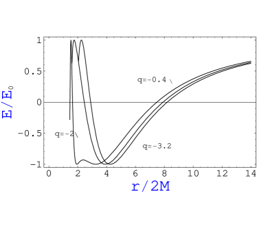
Figure 2: The radial dependence of the dimensionless quantity $\epsilon$ for different values of the dimensionless brane tension.

4 Nonlinear Plasma Modes Along the Field Lines

In this section we consider nonlinear plasma modes along the open field lines around a rotating magnetized neutron star in braneworld. The system of equations governing the nonlinear modes can be written as

$$\frac{\partial}{\partial t^{\prime}}(n_{s})+\nabla\cdot\left(\sqrt{1-\frac{2M}{r}+\frac{Q^{*}}{r^{2}}}n_{s}v_{s}\right)=0,$$ (48)

$$\left(\frac{\partial}{\partial t^{\prime}}+\sqrt{1-\frac{2M}{r}+\frac{Q^{*}}{r^{2}}}v_{s}\cdot\nabla\right)v_{s}=-\frac{e_{s}}{m}\nabla\Phi\ ,$$ (49)

$$\nabla\cdot\left[\left(1-\frac{2M}{r}+\frac{Q^{*}}{r^{2}}\right)^{-\frac{1}{2}}\nabla\Phi\right]=$$

$$\ \ -4\pi\left(\sum_{s}n_{s}e_{s}-\rho_{GJ}\right).$$ (50)

Now for simplicity one may consider $v_{s}\cdot\nabla=v_{sr}\partial/\partial r$ (i.e., one-dimensional wave propagation along $r$) and introduce a moving frame $\tilde{\eta}=r-Vt^{\prime}$, where $V$ is a constant. In the considered moving frame, from equations (48) and (49) we get

$$n_{s}=\frac{n_{0}V}{V-(1-2M/r+Q^{*}/r^{2})^{1/2}v_{s\tilde{\eta}}}\ ,$$ (51)

$$v_{s\tilde{\eta}}-\frac{1}{mV}\left(q_{s}\Phi+\sqrt{1-\frac{2M}{r}+\frac{Q^{*}}{r^{2}}}\frac{e^{2}}{2mV^{2}}\Phi^{2}\right).$$ (52)

Using equations (51) and (52), in equation (50) we derive the nonlinear equation for the plasma mode along the field line of the rotating neutron star in braneworld:

$$4\pi\sqrt{\tilde{A}}\rho_{GJ}=\frac{d^{2}\Phi}{\tilde{\eta}^{2}}-\frac{M}{\tilde{A}\tilde{\eta}^{2}}\frac{d\Phi}{d\tilde{\eta}}+$$

$$\hskip 28.45274pt\frac{\omega^{2}_{p0}\tilde{A}}{V^{2}}\frac{\Phi}{1-2\tilde{A}\left(\frac{e\Phi}{mV^{2}}\right)^{2}+\frac{1}{4}\tilde{A}^{2}\left(\frac{e\Phi}{mV^{2}}\right)^{4}}\ ,$$ (53)

where $\tilde{A}=1-\frac{2M}{\tilde{\eta}}+\frac{Q^{*}}{\tilde{\eta}^{2}}$

Now, introducing dimensionless quantities

$$\bar{\Phi}=\frac{e\Phi}{mV^{2}},\qquad\bar{\eta}=\frac{\tilde{\eta}}{M},$$

$$\bar{\omega}_{p0}=\frac{2M\omega_{p0}}{V}\ ,\qquad\bar{A}=1-\frac{1}{\bar{\eta}}+\frac{q}{\bar{\eta}^{2}}$$ (54)

one can easily rewrite the equation (53)

$$\frac{d^{2}\bar{\Phi}}{d\bar{\eta}^{2}}+\omega_{p0}^{2}\bar{A}\frac{\bar{\Phi}}{1-2\bar{A}\bar{\Phi}^{2}+1/4\bar{A}^{2}\bar{\Phi}^{4}}$$

$$\qquad-\frac{1}{\bar{\eta}^{2}}A^{-1}\frac{d\bar{\Phi}}{d\bar{\eta}}=\frac{\pi e}{mV^{2}M^{2}}A^{-1/2}\rho_{GJ}$$ (55)

We numerically solve equation (55) in the polar cap region ($\theta\simeq 0$) of a neutron star subject to the appropriate boundary conditions. Following Goldreich & Julian (1969) and Muslimov & Harding (1997), we assume that the surface of a polar cap and that formed by the last open field lines can be treated as electric equipotentials. We therefore adopt the condition $\Phi(r=R)=0$. Second, we require that the steady state component of the electric field parallel to the magnetic field vanishes at the polar cap surface, i.e., $d\Phi(r=R)/d\tilde{\eta}=0$. The boundary conditions can be written as $\Phi(2)=\Phi^{\prime}(2)=0$. The solution of equation (55) for the different values of brane tension with the mentioned boundary condition is shown graphically in Fig. 3. It is shown that the Goldreich-Julian charge density creates the initial potential on the surface. Near the radius the potential is enhanced, and it propagates almost without damping along the field lines in the presence of the brane charge. The increasing the module of the brane charge causes to increasing the amplitude of the nonlinear plasma modes.

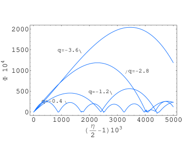
Figure 3: Nonlinear plasma modes in branworld scenario; propagation of the nonlinear plasma modes near the surface of the neutron star.

5 Charged Particle Acceleration in the Polar Cap of A Slowly Rotating Star in Branewold

The origin of radio emission from the polar cap is one of the most mysterious of the remaining unsolved questions in the physics of pulsars. One likely scenario is that particles are accelerated along open magnetic field lines and emit $\gamma$-rays that subsequently convert into electron-positron pairs in the strong magnetic field. The combination of the primary beam and the pair plasma then provides the mechanism of radio emission. For this reason, it is interesting to study particle acceleration conditions and the equations of motion in the pulsar magnetosphere in braneworld models.

In the previous sections the effects of brane parameter on plasma modes along the open field lines of a rotating, magnetized neutron star are studied. In the paper [46] the detail analyze of the motion of the charged particle for a rotating pulsar polar cap has been considered. Now we investigate the charged particles acceleration in the region just above the polar cap surface of a neutron star with brane charge.

Charges $e$ of the same sign as $\rho_{GJ}$ are extracted from the polar cap and carry current $j$. We assume that this charge-separated flow is freely supplied by the star with initial velocity $v\ll c$ and neglect a binding energy of charges at the surface. We will look for a steady state. All particles are in the ground Landau state and flow along the field lines. The flow is governed by the electric field $E_{\|}$ (parallel to $B$),

$$\frac{dp}{dt}=\frac{eE_{\|}}{mc}\ ,$$ (56)

where the momentum of the particle is given in units of $mc$. And, for the parallel electric field $E_{\|}$ one can obtain the equation

$$\nabla\cdot\mathbf{E}=\frac{dE_{\|}}{dz}=4\pi(\rho-\rho_{GJ}),\qquad z\ll r_{\rm pc}$$ (57)

where $r_{\rm pc}$ is the radius of the polar cap of the star and $z$ is the distance from the stellar surface. Rewriting equation (57) in terms of $d/dt=vd/dz$, $\tilde{a}=j/cj_{GJ}$, $\rho=j/v$, and $v=cp(1+p^{2})^{-1/2}$, one can obtain

$$\frac{dE_{\|}}{dt}=4\pi j\left(1-\frac{\tilde{a}p}{\sqrt{1+p^{2}}}\right)$$ (58)

(see [6]), where

$$\tilde{a}(z)=\tilde{a_{0}}\frac{1-\kappa\left(1-{Q^{*}}/{2zM}\right)}{1-\kappa\left(1-{Q^{*}}/{2zM}\right)\left(1+z/R\right)^{-3}}.$$ (59)

Note that to obtain the expression for $\tilde{a}(z)$ (59) we have used the approximate value of the Goldreich-Julian charge density at the polar cap region as

$$\rho_{GJ}=\frac{1}{2\pi}\frac{B\Omega}{N}\left(1-\frac{\omega}{\Omega}+\frac{\omega}{\Omega}\frac{Q^{*}}{2zM}\right)\ .$$ (60)

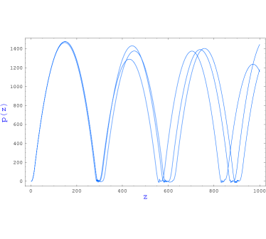
Figure 4: Dependence of the momentum of a charged particle, extracted from polar cap for different value of the brane parameter.

Finally the system of the equations (56), (58), and (59) is solved numerically. In Fig. 4 the dependence of the momentum of a charged particle, extracted from polar cap for different value of the brane parameter are shown. The values of the parameters $B=3\times 10^{12}G$, $P=1s$, $\kappa=0.15$, and $\tilde{a_{0}}=0.999$ are taken from the paper [30]. This dependence shows that the brane charge changes the period of the oscillations.

6 Conclusion

We have considered astrophysical processes in the polar cap of pulsar magnetosphere in space-time of slowly rotating star in the braneworld. In particular, the corrections caused by the brane tension on the Goldreich-Julian charge density, electrostatic scalar potential and accelerating component of electric field being parallel to magnetic field lines in the polar cap region are found. The presence of brane tension slightly modulates Goldreich-Julian charge density near the surface of the star and gives very important additional contribution to the generation of accelerating electric field component in the magnetosphere near the surface of the neutron star.

These results are applied to find an expression for electromagnetic energy losses along the open magnetic field lines of the slowly rotating star in the braneworld. It is found that in the case of non-vanishing brane tension an important contribution to the standard magneto-dipole energy losses expression appears. Comparison of effect of brane tension with the already known effects shows that it can not be neglected. Obtained new dependence may be combined with astrophysical data on pulsar periods slow down and be useful in further investigations on possible detection of the brane tension.

It is also shown that the presence of brane tension has influence on the conditions of particles motion in the polar cap region. From derived results it can be seen, that brane tension modulates the period of oscillations of particle’s momentum. Obtained numerical results can be useful in detecting or getting upper limit for brane parameter by comparing them with astrophysical data on pulsar radiation. As further extension of this research one may consider the propagation of the low-frequency electrostatic wave in a nonuniform electron positron pair magnetoplasma of rotating neutron star containing density, velocity, temperature and magnetic field inhomogeneities [13].

References

- [1] Abdujabbarov, A.A., Ahmedov, B.J.: Phys. Rev. D 81, 044022 (2010)
- [2] Ahmedov, B.J., Fattoyev, F.J.: Phys. Rev. D 78, 047501 (2008)
- [3] Aliev, A.N., Gümrükçüoǧlu, A.E.: Phys. Rev. D 71, 104027 (2005)
- [4] Aliev, A.N., Frolov, V.P.: Phys. Rev. D 69, 084022 (2004)
- [5] Arons, J., Scharlemann, E.T.: ApJ 231, 854 (1979)
- [6] Beloborodov, A.M.: astro-ph/0710.0920v1 (2007)
- [7] Beskin, V.S.: Soviet Astron. Lett. 16, 286 (1990)
- [8] Beskin, V.S.: MHD Flows in Compact Astrophysical Objects: Accretion, Winds and Jets. Extraterrestrial Physics Space Sciences, Springer (2009)
- [9] Böhmer, C.G., Harko, T., Lobo, F.S.N.: Class. Quantum Grav. 25, 045015 (2008)
- [10] Campos, A., Sopuerta, C.F.: Phys. Rev. D 63, 104012 (2001)
- [11] Dadhich, N.K., Maartens, R., Papodopoulos, P., Rezania, V.: Phys. Lett. B 487, 1 (2000)
- [12] Deutsch, A.: Ann. d’Ap. 18, 1 (1955)
- [13] El-Taibany, W.F., Moslem, W.M., Miki Wadati, Shukla, P.K.: Phys. Lett. A 372, 4067 (2008)
- [14] Gergely, L.A.: Phys. Rev. D 74, 024002 (2006)
- [15] Goldreich, P., Julian, W.H.: ApJ 157, 869 (1969)
- [16] Hackman, E., Kagramanova, V., Kunz, J., Lämmerzahl, C.: Phys. Rev. D 78, 124018 (2008)
- [17] Harko, T., Mak, M.K.: Class. Quantum Grav. 20, 407 (2003)
- [18] Kaluza, T.: On The Problem Of Unity In Physics. Sitzungsber. Preuss. Akad. Wiss. Berlin (Math. Phys.), 966-972 (1921)
- [19] Konoplya, R.A.: Phys. Rev. D 74, 124015 (2006)
- [20] Konoplya, R.A.: Phys. Lett. B 644, 219 (2007)
- [21] Kovacs, Z., Gergely, L.A.: Phys. Rev. D 77, 024003 (2008)
- [22] Langlois, D.: Phys. Rev. Lett. 86, 2212 (2001)
- [23] Lavagetto, G., Burderi, L., D’Antona, F., Di Salvo, T., Iaria, R., Robba, N.R.: Mon. Not. R. Astron. Soc. 359, 734 (2005)
- [24] Maartens, R.: Phys. Rev. D 62, 084023 (2000)
- [25] Maartens, R.: Living Reviews in Relativity 7, 1 (2004)
- [26] Majumdar, A.S., Mukherjee, N.: Int. J. Mod. Phys. D 14, 1095 (2005)
- [27] Mamadjanov, A.I., Hakimov, A.A., Tojiev, S.R.: Mod. Phys. Lett. A 25(4), 243 (2010)
- [28] Mestel, L.: Nature 233, 149 (1971)
- [29] Mofiz, U.A., Ahmedov, B.J.: ApJ 542, 484 (2000)
- [30] Morozova, V.S, Ahmedov, B.J., Kagramanova, V.G.: ApJ 684, 1359 (2008)
- [31] Muslimov, A., Harding, A.K.: ApJ 485, 735 (1997)
- [32] Muslimov, A., Tsygan, A.I.: The Magnetospheric Structure and Emission Mechanisms of Radio Pulsars, IAU Colloq. eds Hankins, T., Rankin, J. & Gil, J., Kluwer, Dordrecht No 128, 340 (1991)
- [33] Muslimov, A.G., Tsygan, A.L.: Mon. Not. R. Astr. Soc. 255, 61 (1992)
- [34] Ovalle, J.: Mod. Phys. Lett. A 23, Issue 38, 3247 (2008)
- [35] Page, D., Geppert, U., Zannias, T.: Astron. Astrophys. 360, 1052 (2000)
- [36] Pun, C.S.J., Kovács, Z., Harko, T.: Phys. Rev. D 78, 084015 (2008)
- [37] Randall, L., Sundrum, R.: Phys. Rev. Lett. 83, 3370 (1999a)
- [38] Randall, L., Sundrum, R.: Phys. Rev. Lett. 83, 4690 (1999b,)
- [39] Rezzolla, L., Ahmedov, B.J., Miller, J.C.: Mon. Not. R. Astron. Soc. 322, 723 (2001a); Erratum 338, 816 (2003)
- [40] Rezzolla, L., Ahmedov, B.J., Miller, J.C.: Found. of Phys. 31, 1051 (2001b)
- [41] Rezzolla, L., Ahmedov, B.J.: Mon. Not. R. Astron. Soc. 352, 1161 (2004)
- [42] Ruderman, M., Sutherland, P.G.: ApJ 196, 51 (1975)
- [43] Schee, J., Stuchlík, Z.: Gen. Relativ. Gravit. 41, 1795 (2009a)
- [44] Schee, J., Stuchlík, Z.: Int. J. Mod. Phys. D 18, 983 (2009b)
- [45] Stuchlík, Z., Kotrlová, A.: Gen. Relativ. Gravit. 41, 1305 (2009)
- [46] Sakai, N., Shibata, S.: ApJ 584, 427 (2003)
- [47] Sturrock, P.A.: ApJ 164, 179 (1971)
- [48] Zhu, T., Ruderman, M.: ApJ 478, 701 (1997)