Computing the distance between quantum channels:
Usefulness of the Fano representation

Abstract

The diamond norm measures the distance between two quantum channels. From an operational vewpoint, this norm measures how well we can distinguish between two channels by applying them to input states of arbitrarily large dimensions. In this paper, we show that the diamond norm can be conveniently and in a physically transparent way computed by means of a Monte-Carlo algorithm based on the Fano representation of quantum states and quantum operations. The effectiveness of this algorithm is illustrated for several single-qubit quantum channels.

I introduction

Quantum information processes in a noisy environment are conveniently described in terms of quantum channels, that is, linear, trace preserving, completely positive maps on the set of quantum states qcbook ; nielsen . The problem of discriminating quantum channels is of great interest. For instance, knowing the correct noise model might provide useful information to devise efficient error-correcting strategies, both in the fields of quantum communication and quantum computation.

It is therefore natural to consider distances between quantum channels, that is to say, we would like to quantify how similarly two channels $\mathcal{E}_{1}$ and $\mathcal{E}_{2}$ act on quantum states, or in other words to determine if there are input states $\rho$ on which the two channels produce output states $\rho_{1}^{\prime}=\mathcal{E}_{1}(\rho)$ and $\rho_{2}^{\prime}=\mathcal{E}_{2}(\rho)$ that are distinguishable. The trace norm of $\rho_{1}^{\prime}-\rho_{2}^{\prime}$ represents how well $\rho_{1}^{\prime}$ and $\rho_{2}^{\prime}$ can be distinguished by a measurement helstrom : the more orthogonal two quantum states are, the easier it is to discriminate them. The trace distance of two quantum channels is then obtained after maximizing the trace norm of $\rho_{1}^{\prime}-\rho_{2}^{\prime}$ over the input state $\rho$. However, the trace norm is not a good measure of the distance between quantum channels. Indeed, in general the presence in the input state of entanglement with an ancillary system can help discriminating quantum channels preskill ; acin ; dariano ; sacchi ; sacchi2 . This fact is captured by the diamond norm kitaev ; watrous : the trace distance between the overall output states (including the ancillary system) is optimized over all possible input states, including those entangled.

The computation of the diamond norm is not known to be straightforward and only a limited number of algorithms have been proposed JKP09 ; watrous09 ; BT10 , based on complicated semidefinite programming or convex optimization. On the other hand, analytical solutions are limited to special classes of channels sacchi ; sacchi2 . In this paper, we propose a simple and easily parallelizable Monte-Carlo algorithm based on the Fano representation of quantum states and quantum operations. We show that our algorithm provides reliable results for the case, most significant for present-day implementations of quantum information processing, of single-qubit quantum channels. Furthermore, in the Fano representation quantum operations are described by affine maps whose matrix elements have precise physical meaning: They are directly related to the evolution of the expectation values of the system’s polarization measurements qcbook ; BFS ; BS09 .

The paper is organized as follows. After reviewing in Sec. II basic definitions of the distance between quantum channels, we discuss in Sec. III two numerical Monte-Carlo strategies for computing the diamond norm. The first one is based on the Kitaev’s characterization of the diamond norm. The second one is based on the Fano representation of quantum states and quantum operations. The two methods are compared in Sec. IV for a few physically significant single-qubit quantum channels. Finally, our conclusions are drawn in Sec. V.

II The diamond norm

II.1 Basic definitions

We consider the following problem: given two quantum channels $\mathcal{E}_{1}$ and $\mathcal{E}_{2}$, and a single channel use, chosen uniformly at random from $\{\mathcal{E}_{1},\mathcal{E}_{2}\}$, we wish to maximize the probability of correctly identifying the quantum channel. It seems natural to reformulate the optimization problem into the problem of finding an input state (density matrix) $\rho$ in the Hilbert space $\mathcal{H}$ such that the error probability in the discrimination of the output states $\mathcal{E}_{1}(\rho)$ and $\mathcal{E}_{2}(\rho)$ is minimal. In this case, the minimal error probability reads

$$\begin{array}[]{c}{\displaystyle p_{E}^{\prime}=\frac{1}{2}-\frac{||\mathcal{E}_{1}-\mathcal{E}_{2}||_{1}}{4},}\\ \\ {\displaystyle||\mathcal{E}||_{1}\equiv\max_{\rho}||\mathcal{E}(\rho)||_{1},}\end{array}$$ (1)

where $||X||_{1}\equiv{\rm Tr}\sqrt{X^{\dagger}X}$ denotes the trace norm.

The superoperator trace distance $||\mathcal{E}_{1}-\mathcal{E}_{2}||_{1}$ is, however, not a good definition of the distance between two quantum operations. The point is that in general it is possible to exploit quantum entanglement to increase the distinguishability of two quantum channels. In this case, an ancillary Hilbert space $\mathcal{K}$ is introduced, the input state $\xi$ is a density matrix in $\mathcal{K}\otimes\mathcal{H}$, and the quantum operations are trivially extended to $\mathcal{K}$. That is to say, the output states to discriminate are $(I_{\mathcal{K}}\otimes\mathcal{E}_{1})\xi$ and $(I_{\mathcal{K}}\otimes\mathcal{E}_{2})\xi$, where $\mathcal{I}_{\mathcal{K}}$ is the identity map acting on $\mathcal{K}$. The minimal error probability reads

$$\begin{array}[]{c}{\displaystyle p_{E}=\frac{1}{2}-\frac{||\mathcal{E}_{1}-\mathcal{E}_{2}||_{\diamond}}{4},}\\ \\ {\displaystyle||\mathcal{E}||_{\diamond}\equiv\max_{\xi}||(\mathcal{I}_{\mathcal{K}}\otimes\mathcal{E})\xi||_{1},}\end{array}$$ (2)

where $||\mathcal{E}||_{\diamond}$ denotes the diamond norm of $\mathcal{E}$. It is clear from definition (2) that

$$||\mathcal{E}||_{\diamond}=||\mathcal{I}_{\mathcal{K}}\otimes\mathcal{E}||_{1}\geq||\mathcal{E}||_{1}$$ (3)

and therefore $p_{E}\leq p_{E}^{\prime}$, so that it can be convenient to use an ancillary system to better discriminate two quantum operations after a single channel use. The two quantum channels $\mathcal{E}_{1}$ and $\mathcal{E}_{2}$ become perfectly distinguishable ($p_{E}=0$) when their diamond distance $||\mathcal{E}_{1}-\mathcal{E}_{2}||_{\diamond}=2$.

It turns out that the diamond norm does not depend on $\mathcal{K}$, provided ${\rm dim}(\mathcal{K})\geq{\rm dim}(\mathcal{H})$ kitaev . Due to the convexity of the trace norm, it can be shown that the maximum in both Eqs. (1) and (2) is achieved for pure input states RW05 .

II.2 Kitaev’s characterization of the diamond norm

Kitaev provided a different equivalent characterization of the diamond norm, see, e.g., kitaev ; watrous . Any superoperator (not necessarily completely positive) $\mathcal{E}:L(\mathcal{H})\to L(\mathcal{H})$, with $L(\mathcal{H})$ space of linear operators mapping $\mathcal{H}$ to itself, can be expressed as

$$\mathcal{E}(X)={\rm Tr}_{\mathcal{R}}(AXB^{\dagger}),$$ (4)

where $X\in L(\mathcal{H})$, $A$ and $B$ linear operators from $\mathcal{H}$ to $\mathcal{R}\otimes\mathcal{H}$, with $\mathcal{R}$ auxiliary Hilbert space and ${\rm dim}(\mathcal{R})\leq[{\rm dim}(\mathcal{H})]$. It is then possible to define completely positive superoperators $\Psi_{A},\Psi_{B}:L({\mathcal{H}})\to L({\mathcal{R}})$:

$$\Psi_{A}(X)={\rm Tr}_{\mathcal{H}}(AXA^{\dagger}),\quad\Psi_{B}(X)={\rm Tr}_{\mathcal{H}}(BXB^{\dagger}).$$ (5)

Note that the space ${\mathcal{H}}$ is traced out in the definition of $\Psi_{A}$, $\Psi_{B}$, rather than the space ${\mathcal{R}}$. Finally, it turns out that kitaev ; watrous

$$||\mathcal{E}||_{\diamond}=F_{\rm max}(\Psi_{A},\Psi_{B}),$$ (6)

where $F_{\rm max}(\Psi_{A},\Psi_{B})$ is the maximum output fidelity of $\Psi_{A}$ and $\Psi_{B}$, defined as

$$F_{\rm max}(\Psi_{A},\Psi_{B})=\max_{\rho_{1},\rho_{2}}F[\Psi_{A}(\rho_{1}),\Psi_{B}(\rho_{2})],$$ (7)

where $\rho_{1},\rho_{2}$ are density matrices in $\mathcal{H}$, and the fidelity $F$ is defined as

$$F(\Psi_{A},\Psi_{B})={\rm Tr}\sqrt{\Psi_{A}^{1/2}\Psi_{B}\Psi_{A}^{1/2}}.$$ (8)

Note that $\Psi_{A}$, $\Psi_{B}$ are not density matrices: the conditions ${\rm Tr}(\Psi_{A})=1$, ${\rm Tr}(\Psi_{B})=1$ are not satisfied.

III Computing the diamond norm

We numerically compute the distance (induced by the diamond norm) between two quantum channels $\mathcal{E}_{1}$ and $\mathcal{E}_{2}$ using two Monte-Carlo algorithms. The first one is based on the direct computation of $||\mathcal{E}_{1}-\mathcal{E}_{2}||_{\diamond}$, with the output states $(\mathcal{I}_{\mathcal{K}}\otimes\mathcal{E}_{1})\xi$ and $(\mathcal{I}_{\mathcal{K}}\otimes\mathcal{E}_{2})\xi$ in Eq. (2) computed from $\xi$ taking advantage of the Fano representation of quantum states and quantum operations. The second Monte-Carlo algorithm uses the Kitaev’s representation of the diamond norm to compute the maximum output fidelity $F_{\rm max}$ of Eq. (7). In the following, we will refer to the two above Monte-Carlo algorithms as F-algorithm and K-algorithm, respectively. For the sake of simplicity we will confine ourselves to one-qubit quantum channels, even though the two algorithms can be easily formulated for two- or many-qubit channels.

III.1 The F-algorithm

In this section we describe the F-algorithm, which we will use to directly compute the diamond norm (2), with the maximum taken over a large number of randomly chosen input states $\xi$. A convexity argument shows that it is sufficient to optimize over pure input states $\xi=|\Psi\rangle\langle\Psi|$ RW05 . For one-qubit channels, it is enough to add a single ancillary qubit when computing the diamond norm kitaev . Therefore, we can write

$$|\Psi\rangle=C_{00}|00\rangle+C_{01}|01\rangle+C_{10}|10\rangle+C_{11}|11\rangle,$$ (9)

with

$$\begin{array}[]{l}{\displaystyle C_{00}=\cos\theta_{1}\cos\theta_{2},}\\ {C_{01}=\cos\theta_{1}\sin\theta_{2}e^{i\phi_{1}},}\\ {C_{10}=\sin\theta_{1}\cos\theta_{3}e^{i\phi_{2}},}\\ {C_{11}=\sin\theta_{1}\sin\theta_{3}e^{i\phi_{3}},}\end{array}$$ (10)

where the angles $\theta_{i}\in\left[0,\frac{\pi}{2}\right]$ and the phase $\phi_{i}\in[0,2\pi]$. Hence, the maximization in the diamond norm is over the 6 real parameters $\theta_{1},\theta_{2},\theta_{3}$, and $\phi_{1},\phi_{2},\phi_{3}$. Of course, the number of parameters can be reduced for specific channels when there are symmetries.

Let $\mathcal{E}_{1}$ and $\mathcal{E}_{2}$ denote the two single-qubit superoperators we would like to distinguish. The output states $\xi_{1}^{\prime}\equiv(\mathcal{I}_{\mathcal{K}}\otimes\mathcal{E}_{1})\xi$ and $\xi_{2}^{\prime}\equiv(\mathcal{I}_{\mathcal{K}}\otimes\mathcal{E}_{2})\xi$ can be conveniently computed using the Fano representation. Any two-qubit state can be written in the Fano form as follows fano ; eberly ; mahler :

$$\xi=\frac{1}{4}\sum_{\alpha,\beta=x,y,z,I}R_{\alpha\beta}\sigma_{\alpha}\otimes\sigma_{\beta},$$ (11)

where $\sigma_{x}$, $\sigma_{y}$, and $\sigma_{z}$ are the Pauli matrices, $\sigma_{I}\equiv\openone$, and

$$R_{\alpha\beta}={\rm Tr}[(\sigma_{\alpha}\otimes\sigma_{\beta})\xi].$$ (12)

Note that the normalization condition ${\rm Tr}(\xi)=1$ implies $R_{II}=1$. Moreover, the coefficients $R_{\alpha\beta}$ are real due to the hermicity of $\xi$. Eqs. (11) and (12) allow us to go from the standard representation for the density matrix (in the $\{|0\rangle\equiv|00\rangle,|1\rangle\equiv|01\rangle,|2\rangle\equiv|10\rangle,|3\rangle\equiv|11\rangle\}$ basis) to the Fano representation, and vice versa. It is convenient to write the coefficients $R_{\alpha\beta}$ as a column vector,

$$\begin{array}[]{c}{\bf R}=[R_{xx},R_{xy},R_{xz},R_{xI},R_{yx},R_{yy},\\ \\ R_{yz},R_{yI},R_{zx},R_{zy},R_{zz},R_{zI},R_{Ix},R_{Iy},R_{Iz},R_{II}]^{T}.\end{array}$$ (13)

Then the quantum operations $\mathcal{I}_{\mathcal{K}}\otimes\mathcal{E}_{1}$ and $\mathcal{I}_{\mathcal{K}}\otimes\mathcal{E}_{2}$ map, in the Fano representation, ${\bf R}$ into ${\bf R_{1}^{\prime}}=\mathcal{M}_{1}^{(2)}{\bf R}$ and ${\bf R_{2}^{\prime}}=\mathcal{M}_{2}^{(2)}{\bf R}$, respectively, where $\mathcal{M}_{1}^{(2)}$ and $\mathcal{M}_{2}^{(2)}$ are affine transformation matrices. Such matrices have a simple block structure:

$$\mathcal{M}_{i}^{(2)}=\mathcal{I}^{(1)}\otimes\mathcal{M}_{i}^{(1)},$$ (14)

with $\mathcal{I}^{(1)}$ and $\mathcal{M}_{i}^{(1)}$ $4\times 4$ affine transformation matrices corresponding to the quantum operations $\mathcal{I}_{\mathcal{K}}$ and $\mathcal{E}_{i}$ (of course, $\mathcal{I}^{(1)}$ is the identity matrix). Matrices $\mathcal{M}_{i}^{(1)}$ directly determines the transformation, induced by $\mathcal{E}_{i}$, of the single-qubit Bloch-sphere coordinates $(x,y,x)$. Given the Fano representation for a single qubit, $\rho=\frac{1}{2}\sum_{\alpha}r_{\alpha}\sigma_{\alpha}$, then ${\bf r}=[x,y,z,1]^{T}$ and ${\bf r_{i}^{\prime}}\equiv\mathcal{M}_{i}^{(1)}{\bf r}$. We point out that, while one could compute $\xi_{i}^{\prime}$ from the Kraus representation of the superoperator $\mathcal{I}_{\mathcal{K}}\otimes\mathcal{E}_{i}$, the advantage of the Fano representation is that the matrix elements of $\mathcal{M}_{i}$ are directly related to the transformation of the expectation values of the system’s polarization measurements qcbook ; BFS ; BS09 .

Finally, we compute the trace distance between $\xi_{1}^{\prime}$ and $\xi_{2}^{\prime}$ as

$$||\xi_{1}^{\prime}-\xi_{2}^{\prime}||_{1}=\sum_{k}|\lambda_{k}|,$$ (15)

where $\lambda_{1},...,\lambda_{4}$ are the eigenvalues of $\xi_{1}^{\prime}-\xi_{2}^{\prime}$.

III.2 The K-algorithm

We consider a special and unnormalized state in the extended Hilbert space $\mathcal{K}\otimes\mathcal{H}$:

$$|\alpha\rangle=\sum_{j}|j_{\mathcal{K}}\rangle|j_{\mathcal{H}}\rangle,$$ (16)

where ${\rm dim}(\mathcal{K})={\rm dim}(\mathcal{H})$ and $\{|j_{\mathcal{K}}\rangle\}$, $\{|j_{\mathcal{H}}\rangle\}$ are orthonormal bases for $\mathcal{K}$, $\mathcal{H}$. The state $|\alpha\rangle$ is, up to a normalization factor, a maximally entangled state in $\mathcal{K}\otimes\mathcal{H}$.

We define an operator $\sigma$ on $\mathcal{K}\otimes\mathcal{H}$:

$$\sigma=(\mathcal{I}_{\mathcal{K}}\otimes\mathcal{E})(|\alpha\rangle\langle\alpha|),$$ (17)

where $\mathcal{E}=\mathcal{E}_{1}-\mathcal{E}_{2}$ is the difference of two quantum operations but is not a quantum operation itself. That is, $\mathcal{E}$ is linear but not trace preserving and completely positive.

Using the singular value decomposition of $\sigma$, we can write

$$\sigma=\sum_{i=1}^{M}|u^{(i)}\rangle\langle v^{(i)}|,$$ (18)

where $M$ is the rank of $\sigma$ and $|u^{(i)}\rangle$, $|v^{(i)}\rangle$ are vectors in $\mathcal{K}\otimes\mathcal{H}$. The operator $\sigma$ completely specifies $\mathcal{E}$ and can be exploited to express $\mathcal{E}$ as

$$\mathcal{E}(X)=\sum_{i=1}^{M}A^{(i)}XB^{(i)\dagger}.$$ (19)

The operators $A^{(i)}$ and $B^{(i)}$ can be derived by generalizing the construction of the operator-sum representation for quantum operations (see, for instance, Sec. 8.2.4 in Ref. nielsen ). Given a generic state $|\psi\rangle=\sum_{j}\psi_{j}|j_{\mathcal{H}}\rangle$ in $\mathcal{H}$, we define a corresponding state in $\mathcal{K}$: $|\tilde{\psi}\rangle=\sum_{j}\psi_{j}^{\star}|j_{\mathcal{K}}\rangle$. Next, we define

$$A^{(i)}=\langle\tilde{\psi}|u^{(i)}\rangle.$$ (20)

For instance, in the single-qubit case $|u^{(i)}\rangle=[u^{(i)}_{1},u^{(i)}_{2},u^{(i)}_{3},u^{(i)}_{4}]^{T}$ and we obtain

$$A^{(i)}=\left[\begin{array}[]{cc}u^{(i)}_{1}&u^{(i)}_{3}\\ u^{(i)}_{2}&u^{(i)}_{4}\end{array}\right].$$ (21)

Similarly, we define

$$B^{(i)}=\langle\tilde{\psi}|v^{(i)}\rangle.$$ (22)

Finally, it can be checked that with the above defined operators $A^{(i)}$, $B^{(i)}$ we can express $\mathcal{E}$ by means of Eq. (19).

We can now give explicit expressions for $\Psi_{A}$ and $\Psi_{B}$ in Eq. (5):

$$[\Psi_{A}(X)]_{ij}=\sum_{\alpha,m,n}A^{(i)}_{\alpha m}X_{mn}A^{(j)\star}_{\alpha n},$$ (23)

$$[\Psi_{B}(X)]_{ij}=\sum_{\alpha,m,n}B^{(i)}_{\alpha m}X_{mn}B^{(j)\star}_{\alpha n},$$ (24)

with $1\leq i,j\leq M$. Therefore, $\Psi_{A}$ and $\Psi_{B}$ are $M\times M$ matrices. In the single-qubit case, $M\leq 4$ and to compute the diamond norm through Eq. (7) we need to calculate eigenvalues and eigenvectors of matrices of size $M$. A simpler but less efficient decomposition of $\mathcal{E}$, $\Psi_{A}$, $\Psi_{B}$ is provided in Appendix A.

For single-qubit channels the optimization (7) is over 6 real parameters, 3 for $\rho_{1}$ and 3 for $\rho_{2}$ (for instance, the Bloch-sphere coordinates of $\rho_{1}$ and $\rho_{2}$). As discussed in Sec. III.2, the same number of parameters are needed in the F-method. However, the F-method has computational advantages in that only the eigenvalues of the $4\times 4$ matrix $\xi_{1}^{\prime}-\xi_{2}^{\prime}$ are required, while in the K-method we need to evaluate both eigenvalues and eigenvectors of matrices in general of the same size ($M=4$). Moreover, the singular-values decomposition of matrix $\sigma$ is needed. Besides computational advantages, the F-method is physically more transparent, as it is based on affine maps, whose matrix elements have physical meaning, being directly related to the transformation of the expectation values of the system’s polarization measurements qcbook ; BFS ; BS09 .

IV Examples for single-qubit quantum channels

In this section, we illustrate the working of the F- and K-methods for the case, most significant for present-day implementations, of single-qubit quantum channels.

IV.1 Pauli channels

We start by considering the case of Pauli channels,

$$\mathcal{E}_{i}(\rho)=\sum_{\alpha=x,y,z,I}(q_{\alpha})_{i}\sigma_{\alpha}\rho\sigma_{\alpha},\;\;\;\sum_{\alpha}(q_{\alpha})_{i}=1,\;\;i=1,2,$$ (25)

for which the diamond norm can be evaluated analytically sacchi :

$$||\mathcal{E}||_{\diamond}=||\mathcal{E}_{1}-\mathcal{E}_{2}||_{\diamond}=\sum_{\alpha}|(q_{\alpha})_{1}-(q_{\alpha})_{2}|,$$ (26)

this value of the diamond norm being achieved for maximally entangled input states. The Pauli-channel case will serve as a testing ground for the F- and K-algorithms and help us develop a physical and geometrical intuition.

Let us focus on a couple of significant examples. We first consider the bit-flip and the phase-flip channels:

$$\begin{array}[]{l}{\displaystyle\mathcal{E}_{1}(\rho)=\frac{1+c_{1}}{2}\rho+\frac{1-c_{1}}{2}\sigma_{x}\rho\sigma_{x},}\\ \\ {\displaystyle\mathcal{E}_{2}(\rho)=\frac{1+c_{2}}{2}\rho+\frac{1-c_{2}}{2}\sigma_{z}\rho\sigma_{z},}\end{array}$$ (27)

with $0\leq c_{1},c_{2}\leq 1$. We then readily obtain from Eq. (26) that

$$||\mathcal{E}||_{\diamond}=||\mathcal{E}_{1}-\mathcal{E}_{2}||_{\diamond}=\max\{1-c_{1},1-c_{2}\}.$$ (28)

For this example, the diamond norm coincides with the trace norm, $||\mathcal{E}||_{\diamond}=||\mathcal{E}||_{1}$, and therefore has a simple geometrical interpretation: For a single qubit the trace distance between two single-qubit states is equal to the Euclidean distance between them on the Bloch ball nielsen . Superoperators $\mathcal{E}_{1}$ and $\mathcal{E}_{2}$ map the Bloch sphere into an ellipsoid with $x$ (for the bit-flip channel) and $z$ (for the phase-flip channel) as symmetry axis. If we call $(x,y,z)$, $(x_{1}^{\prime},y_{1}^{\prime},z_{1}^{\prime})$, and $(x_{2}^{\prime},y_{2}^{\prime},z_{2}^{\prime})$, the initial Bloch-sphere coordinates and the new coordinates after application of quantum operations $\mathcal{E}_{1}$ and $\mathcal{E}_{2}$, respectively, we obtain

$$\begin{array}[]{l}x_{1}^{\prime}=x,\;\;y_{1}^{\prime}=c_{1}y,\;\;z_{1}^{\prime}=c_{1}z,\\ \\ x_{2}^{\prime}=c_{2}x,\;\;y_{2}^{\prime}=c_{2}y,\;\;z_{2}^{\prime}=z.\end{array}$$ (29)

The geometrical meaning of the trace norm for the present example is clear from Fig. 1: the length of the line segment $\overline{\rho\rho_{2}^{\prime}}=\overline{\rho_{1}^{\prime}\rho_{2}^{\prime}}$ is the trace (and the diamond) distance $||\mathcal{E}_{1}-\mathcal{E}_{2}||_{1}=||\mathcal{E}_{1}-\mathcal{E}_{2}||_{\diamond}$ (note that in this figure $1-c_{2}>1-c_{1}$).

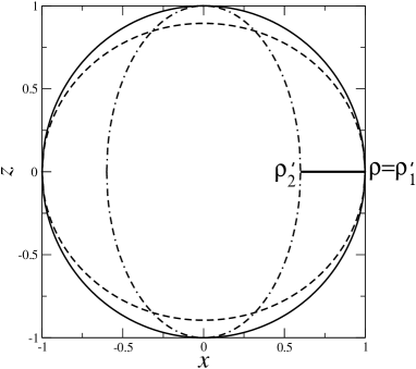
Figure 1: Schematic drawing of the trace (and diamond) distance distance between the bit-flip and the phase-flip channels.

As a further example, we discuss a special instance of the channels considered in Ref. sacchi :

$$\begin{array}[]{l}{\displaystyle\mathcal{E}_{1}(\rho)=\frac{1}{2}\rho+\frac{1}{4}\sigma_{x}\rho\sigma_{x}+\frac{1}{4}\sigma_{y}\rho\sigma_{y},}\\ \\ {\displaystyle\mathcal{E}_{2}(\rho)=\sigma_{z}\rho\sigma_{z}.}\end{array}$$ (30)

In this case,

$$\begin{array}[]{l}{\displaystyle x_{1}^{\prime}=\frac{1}{2}x,\;\;y_{1}^{\prime}=\frac{1}{2}y,\;\;z_{1}^{\prime}=0,}\\ \\ x_{2}^{\prime}=-x,\;\;y_{2}^{\prime}=-y,\;\;z_{2}^{\prime}=z.\end{array}$$ (31)

The trace norm $||\mathcal{E}||_{1}=\frac{3}{2}$, as shown in Fig. 2, where $||\mathcal{E}||_{1}$ is given by the length of the segment $\overline{\rho_{1}^{\prime}\rho_{2}^{\prime}}$. On the other hand, the two channels $\mathcal{E}_{1}$ and $\mathcal{E}_{2}$ are perfectly distinguishable, as we readily obtain from Eq. (26) that $||\mathcal{E}||_{\diamond}=2$, this value being achieved by means of maximally entangled input states. Therefore, in this example $||\mathcal{E}||_{\diamond}>||\mathcal{E}||_{1}$, that is, entangled input states improve the distinguishability of the two channels.

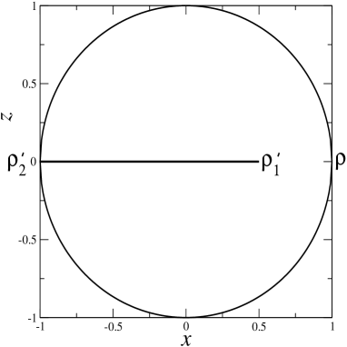
Figure 2: Schematic drawing of the trace distance distance between the two Pauli channels of Eq. (30).

Channels (30) are very convenient to illustrate the convergence properties of the F- and K-algorithms. Let us first consider the F-algorithm. If the maximum of $||\xi_{1}^{\prime}-\xi_{2}^{\prime}||_{1}$, with $\xi_{i}^{\prime}=(\mathcal{I}_{\mathcal{K}}\otimes\mathcal{E}_{i})\xi$ ($i=1,2$) is taken over $N_{r}$ random initial conditions, then the obtained value differs from the diamond norm $||\mathcal{E}||_{\diamond}$ by an amount $\delta(N_{r})$ which must converge to zero when $N_{r}\to\infty$. To get convergence to $||\mathcal{E}||_{\diamond}$ for channels (30) it is enough to optimize over real initial conditions. Numerical results, shown in Fig. 3 for a few runs, are consistent with $\delta(N_{r})\sim 1/N_{r}$. A rough argument can be used to explain the $1/N_{r}$ dependence. Assuming a smooth quadratic dependence of the distance $D(\xi)\equiv||\xi_{1}^{\prime}-\xi_{2}^{\prime}||_{1}$ on the parameters for optimization [the angles $\theta_{i}$ in (10), with $\theta_{1}\in\left[0,\frac{\pi}{2}\right]$, $\theta_{2},\theta_{2}\in[0,2\pi)$] for $\xi$ around the value $\xi_{0}$ optimizing $D$, then $|D(\xi)-D(\xi_{0})|\sim\delta$ when the distance between $\xi$ and $\xi_{0}$ is of the order of $\sqrt{\delta}$. The number $N_{r}$ of randomly distributed initial conditions typically requested to get a point satisfying $||\xi-\xi_{0}||_{1}<\sqrt{\delta}$ is of the order of $(1/\sqrt{\delta})^{n_{p}}$, where $n_{p}$ is the number of parameters for optimization. Therefore, $\delta(N_{r})\sim(1/N_{r})^{2/\delta}$. In the example of Fig. 3, $n_{p}=3$ leading to $\delta(N_{r})\sim(1/N_{r})^{2/3}$. On the other hand, numerical data exhibit a $1/N_{r}$ dependence. This fact has a simple explanation: the maximum is achieved for Bell states, which are invariant under rotations. Hence, the maximum distance is obtained not on a single point but on a curve and the number $N_{r}$ of initial conditions requested to get a point within a trace distance smaller than $\sqrt{\delta}$ from this curve is of the order of $(1/\sqrt{\delta})^{n_{p}-1}$, thus leading to $\delta(N_{r})\sim 1/N_{r}$.

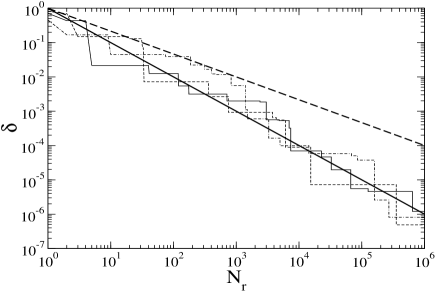
Figure 3: Error $\delta$ in evaluating the diamond distance between channels (30) by means of the F-algorithm after $N_{r}$ randomly chosen initial conditions. Three different runs are shown, together with the $1/N_{r}$ (full line) and $(1/N_{r})^{2/3}$ (dashed line) dependences.

With regard to the K-algorithm, we have observed in the example of Eq. (30) the same $1/N_{r}$ convergence to the expected asymptotic value $||\mathcal{E}||_{\diamond}=2$. However, the cost per initial condition in the K-algorithm is much larger than in the F-algorithm, in agreement with the general discussion of Sec. III.2. Furthermore, the physical meaning of the F-method is much more transparent. For instance, for the Pauli channels (25) the affine transformation matrix $\mathcal{M}_{i}^{(1)}$ such that ${\bf R_{i}^{\prime}}=(\mathcal{I}^{(1)}\otimes\mathcal{M}_{i}^{(1)}){\bf R}$ has a simple diagonal structure:

$$\mathcal{M}_{i}^{(1)}={\rm diag}[(c_{x})_{i},(c_{y})_{i},(c_{z})_{i},1],$$ (32)

where

$$\begin{array}[]{l}(c_{x})_{i}=1-2[(q_{y})_{i}+(q_{z})_{i}],\\ \\ (c_{y})_{i}=1-2[(q_{z})_{i}+(q_{x})_{i}],\\ \\ (c_{z})_{i}=1-2[(q_{x})_{i}+(q_{y})_{i}].\end{array}$$ (33)

Matrix $\mathcal{M}_{i}^{(1)}$ simply accounts for the transformation, induced by $\mathcal{E}_{i}$, of the polarization measurements for the system qubit: $\alpha_{i}^{\prime}=(c_{\alpha})_{i}\alpha$, with $\alpha=x,y,z$ Bloch-sphere coordinates.

We have checked the computational advantages of the F-method also for all the other examples discussed in this paper. For this reason in what follows we shall focus on this method only.

IV.2 Nonunital channels

In this section, we consider nonunital channels, that is, channels that do not preserve the identity. Therefore, in contrast to the Pauli channels considered in Sec. IV.1, single-qubit nonunital channels displace the center of the Bloch sphere. Such channel are physically relevant in the description, for instance, of energy dissipation in open quantum systems, the simplest case being the amplitude damping channel nielsen ; qcbook .

As a first illustrative example, we compute the distance between two channels $\mathcal{E}_{1}$ and $\mathcal{E}_{2}$ corresponding to displacements of the Bloch sphere along the $+x$- and $+z$-direction BFS . In the Fano representation the affine transformation matrices $\mathcal{M}_{i}^{(1)}$ corresponding to maps $\mathcal{E}_{i}$ have a simple structure:

$$\mathcal{M}_{1}^{(1)}=\left[\begin{array}[]{cccc}C_{x}^{2}&0&0&S_{x}^{2}\\ 0&C_{x}&0&0\\ 0&0&C_{x}&0\\ 0&0&0&1\end{array}\right],$$ (34)

$$\mathcal{M}_{2}^{(1)}=\left[\begin{array}[]{cccc}C_{z}&0&0&0\\ 0&C_{z}&0&0\\ 0&0&C_{z}^{2}&S_{z}^{2}\\ 0&0&0&1\end{array}\right],$$ (35)

where we have used the shorthand notation $C_{x}\equiv\cos\theta_{x}$ and $C_{z}\equiv\cos\theta_{z}$. The two channels depend parametrically on $\theta_{x},\theta_{z}\in\left[0,\frac{\pi}{2}\right]$. The limiting cases $\theta_{x}=0$ and $\theta_{z}=0$ correspond to $\mathcal{E}_{1}=\mathcal{I}$ and $\mathcal{E}_{2}=\mathcal{I}$, respectively. Moreover, for $\theta_{x}=\frac{\pi}{2}$ quantum operation $\mathcal{E}_{1}$ maps the Bloch ball onto the single point $(x_{1}^{\prime}=1,y_{1}^{\prime}=0,z_{1}^{\prime}=0)$; for $\theta_{z}=\frac{\pi}{2}$ the mapping operated by $\mathcal{E}_{2}$ is onto the north pole of the Bloch sphere, $(x_{2}^{\prime}=0,y_{2}^{\prime}=0,z_{2}^{\prime}=1)$.

The numerically computed trace distance $||\mathcal{E}_{1}-\mathcal{E}_{2}||_{1}$ is shown in Fig. 4, as a function of the parameters $\theta_{x}$ and $\theta_{z}$. We gathered numerical evidence that for such channels the diamond distance equals the trace distance.

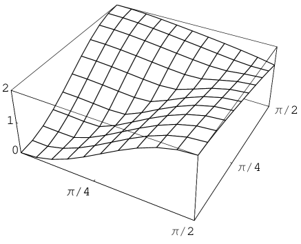
Figure 4: Trace norm $||\mathcal{E}||_{1}=||\mathcal{E}_{1}-\mathcal{E}_{2}||_{1}$, where $\mathcal{E}_{1}$ and $\mathcal{E}_{2}$ are displacement channels along the $+x$- and $+z$-axis of the Bloch sphere.

It is interesting to examine the analytical solutions for two limiting cases: (i) $\theta_{x}=0$ (the case $\theta_{z}=0$ is analogous) and (ii) $\theta_{x}=\theta_{z}=\frac{\pi}{2}$. In the first case, $\mathcal{E}_{1}$ maps the Bloch sphere into an ellipsoid with $z$ as symmetry axis BFS , while $\mathcal{E}_{2}=\mathcal{I}$. The trace norm is given by the length of the line segment $\overline{\rho\rho_{2}^{\prime}}=\overline{\rho_{1}^{\prime}\rho_{2}^{\prime}}$ shown in Fig. 5 (left),

$$||\mathcal{E}||_{1}=2\sin^{2}\theta_{z}.$$ (36)

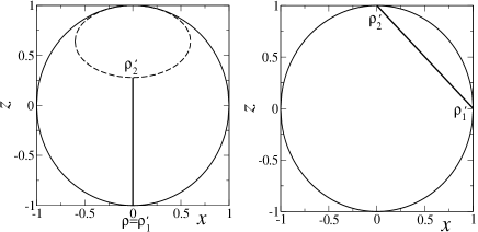
Figure 5: Bloch-sphere visualization of the trace norm $||\mathcal{E}||_{1}$ in the limiting cases $\theta_{x}=0$ (left) and $\theta_{x}=\theta_{z}=\frac{\pi}{2}$ (right).

It is interesting to remark that, in contrast to the Pauli channels, the optimal input state is not a maximally entangled input state. In the limiting case (i) the channels are strictly better discriminated by means of an appropriate separable input state, i.e., the south pole of the Bloch sphere (see the left plot of Fig. 5)) rather than by Bell states. Indeed, given the maximally entangled input state

$$\xi=|\Psi\rangle\langle\Psi|,\quad|\Psi\rangle=\frac{1}{\sqrt{2}}\,(|00\rangle+|11\rangle),$$ (37)

we obtain

$$\xi_{1}^{\prime}-\xi_{2}^{\prime}=\frac{1}{2}\,\left[\begin{array}[]{cccc}0&0&0&C_{z}-1\\ 0&0&0&0\\ 0&0&S_{z}^{2}&0\\ C_{z}-1&0&0&-S_{z}^{2}\end{array}\right].$$ (38)

The trace distance between $\xi_{1}^{\prime}$ and $\xi_{2}^{\prime}$ is then computed by means of Eq. (15):

$$\begin{array}[]{c}{\displaystyle||\xi_{1}^{\prime}-\xi_{2}^{\prime}||_{1}=\frac{S_{z}^{2}}{2}+\,\frac{\left|S_{z}^{2}+\sqrt{S_{z}^{4}+4(1-C_{z})^{2}}\right|}{4}}\\ \\ {\displaystyle+\frac{\left|S_{z}^{2}-\sqrt{S_{z}^{4}+4(1-C_{z})^{2}}\right|}{4}.}\end{array}$$ (39)

As shown in Fig. 6, $||\xi_{1}^{\prime}-\xi_{2}^{\prime}||_{1}<||\mathcal{E}||_{1}$ for any $C_{z}>0$.

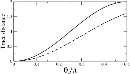
Figure 6: Comparison between $||\mathcal{E}_{1}-\mathcal{E}_{2}||_{1}$ (upper curve) and $||\xi_{1}^{\prime}-\xi_{2}^{\prime}||_{1}$ (lower curve) for $\theta_{x}=\frac{\pi}{2}$.

In case (ii), for any initial state $\rho$, the Bloch coordinates of $\rho_{1}^{\prime}$ and $\rho_{2}^{\prime}$ are given by $(1,0,0)$ and $(0,0,1)$. The trace norm is given by the distance between these two points, $||\mathcal{E}||_{1}=\sqrt{2}$ [see Fig. 5 (right)]. In this case, given an input Bell state or any other two-qubit input state $\xi$, the trace distance $||\xi_{1}^{\prime}-\xi_{2}^{\prime}||_{1}=\sqrt{2}=||\mathcal{E}||_{1}$. Thus, there is no advantage in using an ancillary system.

As a further example, we compute the distance between the depolarizing channel $\mathcal{E}_{1}$ and the nonunital channel $\mathcal{E}_{2}$ corresponding to the displacement along the $+z$-axis of the Bloch sphere. The depolarizing channel belongs to the class of Pauli channels (25), with $q_{I}=1-p$ and $q_{x}=q_{y}=q_{z}=\frac{p}{3}$. This channel contracts the Bloch sphere by a factor $\left(1-\frac{4}{3}p\right)$, with $0\leq p\leq\frac{3}{4}$.

Fig. 7 shows the numerically computed $||\mathcal{E}||_{1}$ and $||\mathcal{E}||_{\diamond}$ as well as their difference $||\mathcal{E}||_{\diamond}-||\mathcal{E}||_{1}$. The use of an ancillary qubit improves the distinguishability of the two channels. However, we remark again that maximally entangled input states can be detrimental. For instance, in the limiting case $p=0$, $\theta_{z}=\frac{\pi}{2}$ we obtain from Eqs. (36) and (39) $||\mathcal{E}||_{1}=2>||\xi_{1}^{\prime}-\xi_{2}^{\prime}||_{1}=\frac{1+\sqrt{5}}{2}$. A clear advantage is instead seen in another limiting case, $p=\frac{3}{4}$, $\theta_{z}=0$. The fully depolarizing channel maps each point of the Bloch ball onto its center, so that the trace distance is given by the radius of the Bloch sphere, $||\mathcal{E}_{1}-\mathcal{E}_{2}||_{1}=1$. On the other hand, by means of Eq. (26) we obtain $||\mathcal{E}_{1}-\mathcal{E}_{2}||_{\diamond}=\frac{3}{2}$.

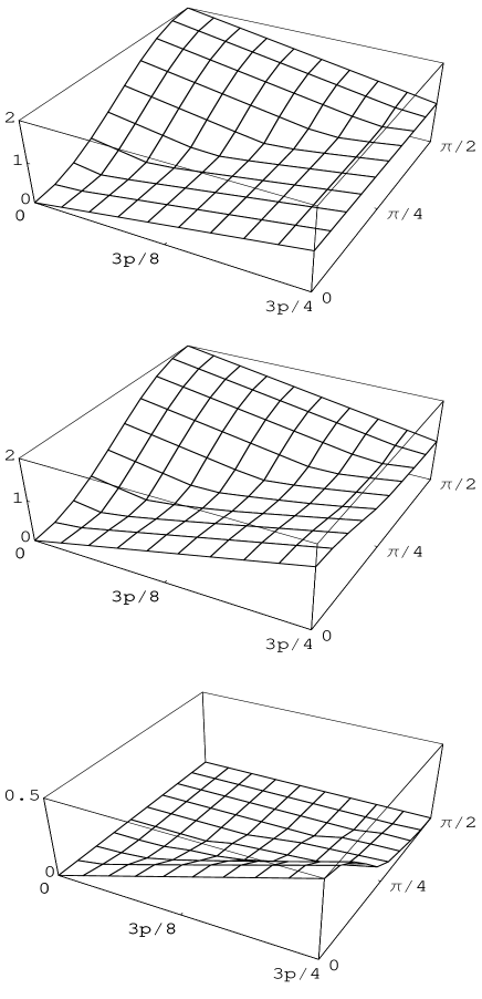
Figure 7: From top to bottom: trace norm $||\mathcal{E}||_{1}=||\mathcal{E}_{1}-\mathcal{E}_{2}||_{1}$, diamond norm $||\mathcal{E}||_{\diamond}$, and their difference $||\mathcal{E}||_{\diamond}-||\mathcal{E}||_{1}$; $\mathcal{E}_{1}$ is the depolarizing channel, $\mathcal{E}_{2}$ the displacement along the $+z$-axis of the Bloch sphere.

V Conclusions

We have shown that the distance between two quantum channels can be conveniently computed by means of a Monte-Carlo algorithm based on the Fano representation. The effectiveness of this algorithm is illustrated in the case, most relevant for present-day implementations of quantum information processing, of single-qubit quantum channels. A main computational advantage of this algorithms is that it is easily parallelizable. Furthermore, being based on the Fano representation, is enlights the physical meaning of the involved quantum channels: the matrix elements of the affine map representing a quantum channel directly account for the evolution of the expectation values of the system’s polarization measurements. More generally, we believe that the Fano representation provides a computationally convenient and physically trasparent representation of quantum noise.

Appendix A Alternative decomposition of $\mathcal{E}$

Given a superoperator $\mathcal{E}=\mathcal{E}_{1}-\mathcal{E}_{2}$, with $\mathcal{E}_{1}$, $\mathcal{E}_{2}$ quantum operations, we start from the Kraus representation qcbook ; nielsen of $\mathcal{E}_{1}$ and $\mathcal{E}_{2}$:

$$\mathcal{E}_{1}(X)=\sum_{k=1}^{M_{1}}E_{k}XE_{k}^{\dagger},\quad\mathcal{E}_{2}(X)=\sum_{k=1}^{M_{2}}F_{k}XF_{k}^{\dagger},$$ (40)

and define new operators:

$$\begin{array}[]{l}{\displaystyle\tilde{A}^{(2k-1)}=\frac{1}{\sqrt{2}}(F_{k}+G_{k}),\quad\tilde{A}^{(2k)}=\frac{1}{\sqrt{2}}(F_{k}-G_{k}),}\\ \\ {\displaystyle\tilde{B}^{(2k-1)}=\tilde{A}^{(2k)},\quad\tilde{B}^{(2k)}=\tilde{A}^{(2k-1)},}\end{array}$$ (41)

where $k=1,...,\overline{M}\equiv\max(M_{1},M_{2})$. Note that, if $M_{1}>M_{2}$, we set $G_{k}=0$ for $k=M_{2}+1,...,M_{1}$; vice-versa, if $M_{1}<M_{2}$, $F_{k}=0$ for $k=M_{1}+1,...,M_{2}$. It is easy to see that

$$\mathcal{E}(X)=\sum_{i=1}^{2\overline{M}}\tilde{A}^{(i)}X\tilde{B}^{(i)\dagger}.$$ (42)

In contrast to (19), the present decomposition of $\mathcal{E}(X)$ is simpler, in that no singular value decomposition is required, but less efficient. Indeed, the maximum number of terms in (42) is twice that of decomposition (19). This implies that, if $\Psi_{A}$, $\Psi_{B}$ are expressed in terms of operators $\tilde{A}^{(i)}$, $\tilde{B}^{(i)}$ rather than $A^{(i)}$, $B^{(i)}$, to evaluate $F(\Psi_{A},\Psi_{B})$ we need to compute eigenvalues and eigenvectors of matrices of size $2\overline{M}$. In the single-qubit case, typically $2\overline{M}=8$.

- (1) G. Benenti, G. Casati, and G. Strini, Principles of Quantum Computation and Information, Vol. I: Basic concepts (World Scientific, Singapore, 2004); Vol. II: Basic tools and special topics (World Scientific, Singapore, 2007).
- (2) M. A. Nielsen and I. L. Chuang, Quantum Computation and Quantum Information (Cambridge University Press, Cambridge, 2000).
- (3) C. W. Helstrom, Quantum Detection and Estimation Theory (Academic, New York, 1976).
- (4) A. M. Childs, J. Preskill, and J. Renes, J. Mod. Opt. 47, 155 (2000).
- (5) A. Acín, Phys. Rev. Lett. 87, 177901 (2001).
- (6) G. M. D’Ariano, P. Lo Presti, and M. G. A. Paris, Phys. Rev. Lett. 87, 270404 (2001).
- (7) M. F. Sacchi, Phys. Rev. A 71, 062340 (2005); ibid. 72, 014305 (2005).
- (8) G. M. D’Ariano, M. F. Sacchi, and J. Kahn, Phys. Rev. A 72, 052302 (2005).
- (9) A. Yu. Kitaev, A. H. Shen, and M. N. Vyalyi, Classical and Quantum Computation, vol. 47 of Graduate Studies in Mathematics (American Mathematical Society, Providence, Rhode Island, 2002), Sec. 11.
- (10) J. Watrous, Advanced Topics in Quantum Information Processing, chap. 22, Lecture notes (2004), at http://www.cs.uwaterloo.ca/watrous/lecture-notes/701/.
- (11) N. Johnston, D. W. Kribs, and V. I. Paulsen, Quantum Inf. Comput. 9, 16 (2009).
- (12) J. Watrous, Theory of Computing 5, 11 (2009).
- (13) A. Ben-Aroya and A. Ta-Shma, Quantum Inf. Comput. 10, 87 (2010).
- (14) G. Benenti, S. Felloni, and G. Strini, Eur. Phys. J. D 38, 389 (2006).
- (15) G. Benenti and G. Strini, Phys. Rev. A 80, 022318 (2009).
- (16) B. Rosgen and J. Watrous, in Proceedings of the 20th Annual Conference on Computational Complexity, pages 344-354 (2005), preprint arXiv:cs/0407056.
- (17) U. Fano, Rev. Mod. Phys. 29, 74 (1957); ibid. 55, 855 (1983).
- (18) F. T. Hioe and J. H. Eberly, Phys. Rev. Lett. 47, 838 (1981).
- (19) J. Schlienz and G. Mahler, Phys. Rev. A 52, 4396 (1995).