Thermodynamics and Phase Structure of the Two-Flavor Nambu–Jona-Lasinio Model Beyond Large-$N_{c}$

Abstract

The optimized perturbation theory (OPT) method is applied to the $SU(2)$ version of the Nambu–Jona-Lasinio (NJL) model both at zero and at finite temperature and/or density. At the first nontrivial order the OPT exhibits a class of $1/N_{c}$ corrections which produce nonperturbative results that go beyond the standard large-$N_{c}$, or mean-field approximation. The consistency of the OPT method with the Goldstone theorem at this order is established, and appropriate OPT values of the basic NJL (vacuum) parameters are obtained by matching the pion mass and decay constant consistently. Deviations from standard large-$N_{c}$ relations induced by OPT at this order are derived, for example, for the Gell–Mann-Oakes-Renner relation. Next, the results for the critical quantities and the phase diagram of the model, as well as a number of other thermodynamical quantities of interest, are obtained with OPT and then contrasted with the corresponding results at large $N_{c}$.

I Introduction

Nambu–Jona-Lasinio (NJL) models njl are schematic quark models useful as a tool to understand the physics associated with chiral symmetry and the phase structure in quantum chromodynamics (QCD). NJL types of model are extensively used in studies related to nuclear astrophysics, such as the ones concerning neutron and quark stars, while sophisticated versions of the model are also employed to study color superconducting phases in deconfined quark matter in attempts to unveil the QCD phase diagram (for NJL model reviews, both at zero and at finite temperature and density, see e.g. Refs. klevansky ; njlrev3 ; buballa ).

Since the model does not include gluon degrees of freedom and thus cannot be used to study confinement, its use is more suitable for the study of the low-temperature regime of QCD and quark matter, where the physics of confinement is less important. However, in this regime the strong-coupling and nonperturbative nature of the nuclear matter becomes relevant. Many studies using NJL-type of models have restricted themselves to the use of the large-$N_{c}$ (LN) limit (where $N_{c}$ is the number of colors), which is also equivalent to the Hartree approximation klevansky . Although a number of investigations of higher-order corrections beyond the Hartree approximation have been carried out in the past (see, e.g., nloNc ; oertel in particular for the next-to-leading $1/N_{c}$ calculations), these studies are in general technically involved and not obvious, and they may open new issues. Typically, because of the intrinsic non-renormalisability of the model, going to higher orders requires in general the introduction of new parameters, sometimes making the conclusion and comparison with simpler LN results to depend on extra parameters. It is thus of interest to examine alternative methods able to go beyond mean-field approximations, to determine how they perform as compared to the LN approximation, and whether they provide both qualitatively and quantitatively relevant corrections to the large-$N_{c}$ constraint.

In this paper we consider the simplest $SU(2)$ version of the NJL model that will be exploited beyond the LN limit, or mean-field approximation (MFA), by means of the Optimized Perturbation Theory (OPT). The OPT method (which also goes by different names, or has many variants, e.g. “delta-expansion” early , order-dependent mapping zinn-justin_rev , etc) is notorious for allowing evaluations beyond the MFA because of the way it modifies the ordinary perturbative expansion, giving a nontrivial (nonperturbative) coupling dependence. In particular, in models with an $O(N)$ or $SU(N)$ symmetry, an important part of next-to-leading $1/N$ corrections are captured at first OPT order, although it is basically a different approximation scheme than the $1/N$ expansion, while corrections belonging formally to higher $1/N$ order are also partly included. In the few studied models where perturbative orders are available at high orders, the OPT turns out to improve substantially the convergence of ordinary perturbation, resumming the latter to some extent, and providing convergent sequences of approximations to some nonperturbative results. Examples of successful applications include the precise determination of the critical temperature for weakly interacting dilute Bose gases bec , phase diagrams for scalar theories escalar , Gross-Neveu (GN) types of model prdgn2d ; prdgn3d and Yukawa theories yukawa , as well as the recent precise determination of critical dopant concentration in polyacetylene poly . In particular, the precise location of the tricritical point and the mixed liquid-gas phase within the GN model in 2+1 dimensions prdgn3d illustrates how this method can be a powerful tool beyond standard perturbation theory, since these important effects were missed by the MFA and could not be precisely determined by Monte Carlo simulations mc . Moreover in the $O(N)$ GN model it has been shown very recently optrg that a percentage level of accuracy can be reached already at first OPT and $1/N$-expansion order, when in this case the relevant renormalization group dependence is incorporated. The method has also been recently applied with success to the study of spontaneous supersymmetry breaking susy . Finally, closer to NJL model considerations, the OPT approach has been applied in the past directly to the full QCD Lagrangian (at zero temperature), in a way consistent with renormalization, obtaining, for instance, estimations of the quark condensate and pion decay constant in the chiral symmetry limit qcdopt .

The OPT version adopted here is mainly indicated to nongauge theories, which (at finite temperature) require the method to be extended, for example, by adding and subtracting a hard-thermal-loop improvement that modifies the propagators and vertices in a self-consistent way, in the so-called hard-thermal-loop perturbation theory (HTLPT) HTLPT .

We will see that the OPT method, as applied at first order to the simplest version of the NJL model, does not introduce new effective parameters beyond those present in the standard MFT or LN picture, while providing at the same time nontrivial corrections beyond LN approximation. Applying the OPT to the NJL model actually provides a rather complete description of the thermodynamics of the model, showing how corrections beyond LN change known results at that level of approximation. This allows to pinpoint how important these corrections may be in providing a reliable description for the model. By studying different thermodynamical quantities, like the trace anomaly, specific heat and quark susceptibility, we are also able to understand how useful these quantities might be as indicators for precise location of the critical points in the phase diagram, a topic of most interest today in the context of quark-gluon phase transition and heavy-ion collision experiments.

This paper is organized as follows. In Sec. II we review the basic features of the two-flavor NJL model. In Sec. III we discuss how the OPT has to be implemented within this model. In Sec. IV we evaluate the Landau’s free energy density and its optimization is performed to the first nontrivial order in the OPT. In Sec. V we establish the validity of the Goldstone theorem at this OPT order, and derive all necessary expressions to rederive a consistent set of basic vacuum NJL parameters matched to the pion mass and decay constant. In Sec. VI we present a series of numerical results that are relevant at various regimes of temperature and/or density. The phase diagram of the NJL model, as well as many relevant thermodynamical quantities, are further explored and compared with the corresponding LN approximation results. Our conclusions and perspectives are presented in Sec. VII. Two appendixes are included to give some relevant technical expressions and details of our calculations.

II The two-flavor NJL effective model for quarks

The NJL model is described by a Lagrangian density for fermionic fields given by njl

$$\mathcal{L}={\bar{\psi}}\left(i{\partial\hbox{$\!\!\!/$}}-m_{c}\right)\psi+G\left[({\bar{\psi}}\psi)^{2}+({\bar{\psi}}i\gamma_{5}{\vec{\tau}}\psi)^{2}\right],$$ (1)

where $\psi$ (a sum over flavors and color degrees of freedom is implicit) represents a flavor isodoublet ($u,d$ types of quarks) $N_{c}$-plet quark fields, while $\vec{\tau}$ are isospin Pauli matrices. The Lagrangian density (1) is invariant under (global) $U(2)_{\rm f}\times SU(N_{c})$ and, when $m_{c}=0$, the theory is also invariant under chiral $U(2)_{L}\times U(2)_{R}$. Note that, as emphasized in Refs. koch ; buballa_stab ; buballa , the introduction of a vector interaction term of the form $({\bar{\psi}}\gamma^{\nu}\psi)^{2}$ in Eq. (1) is also allowed by the chiral symmetry and such a term can become important at finite densities, generating a saturation mechanism depending on the vector coupling strength that provides better matter stability. Within the LN approximation (or MFA), the effect of such a term in the thermodynamical potential is to produce a shift on the chemical potential. However, this term will not be considered here.

Due to the quadratic fermionic interaction, the theory is nonrenormalizable in 3+1 dimensions ($G$ has dimensions of $\mathrm{eV}^{-2}$), meaning that divergences appearing at successive perturbative orders cannot be all eliminated by a consistent redefinition of the original model parameters (fields, masses, and couplings). The renormalizability issue arises during the evaluation of momentum integrals associated with loop Feynman graphs in a perturbative expansion and, in the process, one usually employs regularization prescriptions (e.g. dimensional regularization, sharp cutoff, etc) to formally isolate divergences. However, the procedure introduces arbitrary parameters with dimensions of energy that do not appear in the original Lagrangian density. Within the NJL model a sharp cut off ($\Lambda$) is preferred and since the model is nonrenomalizable, one has to fix $\Lambda$ to a value related to the physical spectrum under investigation. This strategy turns the 3+1 NJL model into an effective model, where $\Lambda$ is treated as a parameter, as usual in effective nonrenormalizable field theory models. The experimental values of quantities such as the pion mass ($m_{\pi}$) and the pion decay constant $(f_{\pi})$ are used to fix both, $G$ and $\Lambda$. An interesting alternative regarding regularization within the NJL model is presented in Ref. gastaoNJL (where explicit evaluation of divergent integrals is avoided by assuming in intermediate steps only general symmetry properties of the regularization, such that the finite parts are integrated in a way independent of the regularization).

A second important issue regards the fact that, when $m_{c}=0$, the quark propagator brings unwanted infrared divergences, meaning that the evaluations have to be carried out in a nonperturbative fashion. Moreover, very often physical quantities (like the self-energy) appear as powers of the dimensionless quantity $G\Lambda^{2}$, which is greater than unity, preventing any possibility of calculations via standard perturbative methods.

In analytic nonperturbative evaluations, one can consider one-loop contributions dressed by a fermionic propagator, whose effective mass, $M$, is determined in a self-consistent way. This approximation is known under different names, for example, the Hartree, LN or mean-field approximation. To obtain the effective potential (or Landau free energy density), $\mathcal{F}$, for the quarks, it is convenient to consider the bosonized version of the NJL, which is easily obtained by introducing auxiliary fields ($\sigma,{\vec{\pi}}$) through a Hubbard-Stratonovich type of transformation. Here, $\mathcal{F}$ is evaluated using the LN approximation, which is equivalent to the MFA. Then, to introduce the auxiliary bosonic fields and to render the theory more suitable for use of the LN approximation, it is convenient to use $G\rightarrow\lambda/(2N_{c})$ and to formally treat $N_{c}$ as a large number, which is set to the relevant value, $N_{c}=3$, at the end of the evaluations. One then has

$$\mathcal{L}={\bar{\psi}}\left(i{\partial\hbox{$\!\!\!/$}}-m_{c}\right)\psi-{\bar{\psi}}(\sigma+i\gamma_{5}{\vec{\tau}\cdot}{\vec{\pi}})\psi-\frac{N_{c}}{2\lambda}(\sigma^{2}+{\vec{\pi}}^{2}).$$ (2)

At finite temperature and density the model can be studied in terms of the grand partition function, defined as usual by

$$Z(\beta,\mu)=\mathrm{Tr}\exp\left[-\beta\left(H-\mu Q\right)\right]\;,$$ (3)

where $\beta$ is the inverse of the temperature, $\mu$ is the chemical potential for both flavors, $H$ is the Hamiltonian corresponding to Eq. (2) and $Q=\int d^{3}x\bar{\psi}\gamma_{0}\psi$ is the mean baryon charge.

III Interpolation of the NJL Model

To implement the OPT within the NJL model one follows the prescription used in Refs. prdgn2d ; prdgn3d by first interpolating the original four-fermion version in terms of a fictitious parameter $\delta$, which is the new expansion parameter. For a long, but far from complete list of references on this and related methods, see early ; linear . See also zinn-justin_rev for a recent review. According to this prescription the deformed Lagrangian density for the NJL model in terms of the auxiliary fields becomes

$$\mathcal{L}=\bar{\psi}\left[i{\partial\hbox{$\!\!\!/$}}-m_{c}-\delta\left(\sigma+i{\gamma}_{5}{\vec{\tau}\cdot\vec{\pi}}\right)-\eta\left(1-\delta\right)\right]{\psi}-\delta\frac{N_{c}}{2\lambda}\left(\sigma^{2}+{\vec{\pi}}^{2}\right).$$ (4)

In order to discuss issues related to chiral symmetry breaking (CSB) and Goldstone’s theorem, it is useful to temporarily consider the chiral limit of the original theory by setting $m_{c}=0$. Note then that the actual chiral limit and original Lagrangian is recovered for $\delta\to 1$, and that $\eta$ at this stage is an arbitrary mass parameter, as usual in the OPT method. Now, a well-established result concerning the OPT evaluation of the free energy density (or effective potential), $\mathcal{F}$, in the LN limit, shows that $\bar{\eta}$ becomes exactly the classical value of the background fields, so that both approximations coincide in this limit. For example, if one sets $\pi_{i}=0$ in Eq. (4), the NJL becomes analogous to the GN model, displaying discrete CSB. In this case, numerous applications show that, when considering the LN limit, we obtain $\bar{\eta}=\sigma_{c}$. However, within the NJL model, apart from the scalar channel, one also has to deal with the pseudoscalar channel. This situation was addressed in detail in Ref. firstOPT , where it was shown that the interpolation mass parameter, $\eta$, can be extended to account for arbitrary mass parameters in the pseudoscalar direction. This can be accomplished by redefining $\eta$ in Eq. (4) such that

$$\eta\to\eta+i{\gamma}_{5}{\vec{\tau}\cdot\vec{\beta}},$$ (5)

implying in the most general case, four mass parameters, $\eta$ and the three components of $\vec{\beta}$, to be fixed by a well-defined prescription (optimization) to determine them. However, as the Landau free energy (or equivalently, the effective potential) is concerned, only the fluctuations in the scalar direction become relevant when only the scalar field $\sigma$ acquires a nonzero vacuum expectation value ($\langle\sigma\rangle\equiv\sigma_{c}$ by slight abuse of notation). In other words, one assumes from now on that $\langle\pi_{i}\rangle=0$, which can be shown to imply firstOPT within the OPT that $\bar{\beta}_{i}=0$. Taking this simplest solution, one needs only to consider the simplest variational interpolation involving only one mass parameter $\eta$, as explained below.

Once the free energy density $\mathcal{F}$ is evaluated to a given order $k$ in the OPT, the optimization procedure used to fix the arbitrary mass dependence follows by a specific prescription prdgn3d , such as the principle of minimal sensitivity (PMS) pms ,

$$\left.\frac{d\mathcal{F}^{(k)}}{d\eta}\right|_{\bar{\eta},\delta=1}=0\;.$$ (6)

IV Optimized Free Energy Density

To order $\delta$, Landau’s free energy density is given by the diagrams shown in Fig 1. They are evaluated using OPT dressed propagators, where the mass term, using a compact notation, is given by

$$\hat{\eta}=\eta+m_{c}-\delta\left[\eta-\left(\sigma+i{\gamma}_{5}{\vec{\tau}}\cdot{\vec{\pi}}\right)\right]\;,$$ (7)

whose form is useful to produce results both for $m_{c}\neq 0$ and for the chiral symmetric limit $m_{c}=0$.

Figure 1: Diagrams contributing to $\mathcal{F}\left({\hat{\eta}}\right)$ to order $\delta$. The thick continuous fermionic lines represent $\ {\hat{\eta}}$-dependent terms which must be further expanded. The dashed line represents the $\sigma$ and the $\pi$ is represented by the dashed-doted line. Note that both are nonpropagating at this level of approximation. The first diagram contributes with $1/N_{c}^{0}$, the second and third diagrams (of order $\delta$) contribute with $1/N_{c}$.

In the Feynman diagrams displayed in Fig. 1, the free energy density in the $\sigma_{c}$ direction reads

$$\frac{\mathcal{F}}{N_{c}} = \frac{\sigma_{c}^{2}}{2\lambda}+i\int\frac{d^{4}p}{\left(2\pi\right)^{4}}\mathrm{Tr}\,{\ln\left(p{\hbox{$\!\!\!/$}\mathbf{-}}\eta-m_{c}\right)}+i\int\frac{d^{4}p}{\left(2\pi\right)^{4}}\mathrm{Tr}\left(\frac{\eta-\sigma_{c}}{p{\hbox{$\!\!\!/$}\mathbf{-}}\eta-m_{c}}\right)$$ (8)

$$+\frac{1}{2}\frac{\delta\lambda}{N_{c}}\int\frac{d^{4}p}{\left(2\pi\right)^{4}}\int\frac{d^{4}q}{\left(2\pi\right)^{4}}\mathrm{Tr}\left(\frac{1}{p{\hbox{$\!\!\!/$}}-\eta-m_{c}}\right)\left(\gamma_{5}\tau_{i}\frac{1}{q{\hbox{$\!\!\!/$}}-\eta-m_{c}}\gamma_{5}\tau_{i}\right)$$

$$-\frac{1}{2}\frac{\delta\lambda}{N_{c}}\int\frac{d^{4}p}{\left(2\pi\right)^{4}}\int\frac{d^{4}q}{\left(2\pi\right)^{4}}\mathrm{Tr}\left(\frac{1}{p{\hbox{$\!\!\!/$}}-\eta-m_{c}}\right)\left(\frac{1}{q{\hbox{$\!\!\!/$}}-\eta-m_{c}}\right)\;.$$

The traces in Eq. (8) are over flavor and Dirac matrix indices. Then, after some algebra, one arrives at

$$\frac{\mathcal{F}}{N_{c}} = \frac{\sigma_{c}^{2}}{2\lambda}+2iN_{\rm f}\int\frac{d^{4}p}{\left(2\pi\right)^{4}}{\ln}\left[-p^{2}+(\eta+m_{c})^{2}\right]$$ (9)

$$- 4i\delta N_{\rm f}\int\frac{d^{4}p}{\left(2\pi\right)^{4}}\frac{(\eta+m_{c})\left(\eta-\sigma_{c}\right)}{-p^{2}+(\eta+m_{c})^{2}}$$

$$-2(n_{\pi}+1)\,\frac{\delta\lambda N_{\rm f}}{N_{c}}\left[\int\frac{d^{4}p}{\left(2\pi\right)^{4}}\frac{p_{0}}{-p^{2}+(\eta+m_{c})^{2}}\right]^{2}$$

$$+ 2(n_{\pi}-1)\,\frac{\delta\lambda N_{\rm f}}{N_{c}}\>(\eta+m_{c})^{2}\>\left[\int\frac{d^{4}p}{\left(2\pi\right)^{4}}\frac{1}{-p^{2}+(\eta+m_{c})^{2}}\right]^{2}\;,$$

where $n_{\pi}$ represents the number of pseudoscalars. It is interesting to see the type of loop contributions contained in Eq. (9). First let us consider the $N_{c}^{0}$ contributions. The second term in Eq. (9) corresponds to a gas of free fermions whose mass has been dressed, while the third term represents tadpole-type of contributions, proportional to the quark condensate, $\langle{\bar{\psi}}\psi\rangle$. The $1/N_{c}$ contributions, given by the two last lines in Eq. (9), are proportional to $(2\langle{\psi}^{+}\psi\rangle^{2}-\langle{\bar{\psi}}\psi\rangle^{2})$ where $\langle{\psi}^{+}\psi\rangle=\langle{\bar{\psi}}\gamma^{0}\psi\rangle$ represents the total quark number density. Note also that for the $U(1)$ version of the model, $N_{\rm f}=1$ and $n_{\pi}=1$, so that the last term does not contribute and the OPT will bring $1/N_{c}$ corrections only at finite density. However, for the case under study here $n_{\pi}=3$ and finite $N_{c}$ corrections are expected to occur at any temperature and density regime.

All our momentum integrals are to be interpreted in the Matsubara finite-temperature formalism,

$$\int\frac{d^{4}p}{\left(2\pi\right)^{4}}\equiv\frac{i}{\beta}\sum_{n=-\infty}^{+\infty}\int\frac{d^{3}p}{\left(2\pi\right)^{3}}\;,$$ (10)

and quadrimomenta given as $p=(i\omega_{n}+\mu,{\bf p})$, with $\omega_{n}=(2n+1)\pi T,\;n=0,\pm 1,\pm 2,\ldots$, are the Matsubara frequencies for fermions. The relevant Matsubara’s sums are given in Appendix A. One can now fix $\delta=1$ and optimize $\mathcal{F}$ using the PMS relation, given by Eq. (6). Application of the PMS condition to Eq. (9) gives

$$\frac{d\mathcal{F}}{d\eta}\Bigr{|}_{\bar{\eta},\delta=1} = {-}4iN_{c}N_{\rm f}\int\frac{d^{4}p}{\left(2\pi\right)^{4}}\frac{\left(\bar{\eta}-\sigma_{c}\right)}{-p^{2}+({\bar{\eta}+m_{c})^{2}}}$$ (11)

$${-}4iN_{c}N_{\rm f}\left[(\bar{\eta}+m_{c})\left(\bar{\eta}-\sigma_{c}\right)\right]\frac{d}{d\eta}\left[\int\frac{d^{4}p}{\left(2\pi\right)^{4}}\frac{1}{-p^{2}+(\bar{\eta}+m_{c})^{2}}\right]\Bigr{|}_{\bar{\eta}}$$

$$-16\lambda N_{\rm f}\left[\int\frac{d^{4}p}{\left(2\pi\right)^{4}}\frac{p_{0}}{-p^{2}+({\bar{\eta}+m_{c})^{2}}}\right]\frac{d}{d\eta}\left[\int\frac{d^{4}p}{\left(2\pi\right)^{4}}\frac{p_{0}}{-p^{2}+(\bar{\eta}+m_{c})^{2}}\right]\Bigr{|}_{\bar{\eta}}$$

$$+8\lambda N_{\rm f}(\bar{\eta}+m_{c})^{2}\;\int\frac{d^{4}p}{\left(2\pi\right)^{4}}\frac{1}{-p^{2}+(\bar{\eta}+m_{c})^{2}}\frac{d}{d\eta}\left[\int\frac{d^{4}p}{\left(2\pi\right)^{4}}\frac{1}{-p^{2}+(\bar{\eta}+m_{c})^{2}}\right]\Bigr{|}_{\bar{\eta}}$$

$$+8\lambda N_{\rm f}(\bar{\eta}+m_{c})\left[\int\frac{d^{4}p}{\left(2\pi\right)^{4}}\frac{1}{-p^{2}+(\bar{\eta}+m_{c})^{2}}\right]^{2}=0\;.$$

Now, considering Eq. (9) at finite temperature and chemical potential, we can write it in the more compact form

$${\mathcal{F}} = \frac{\sigma_{c}^{2}}{4G}-2N_{\rm f}N_{c}I_{1}(\mu,T)+2\delta N_{\rm f}N_{c}(\eta+m_{c})\left(\eta-\sigma_{c}\right)I_{2}(\mu,T)$$ (12)

$$+4\delta GN_{\rm f}N_{c}\>I_{3}^{2}(\mu,T)-2\delta GN_{\rm f}N_{c}\,(\eta+m_{c})^{2}I^{2}_{2}(\mu,T)\;,$$

where we have replaced $\lambda\to 2GN_{c}$. In this equation we have defined, for convenience, the following basic relevant integrals:

$$I_{1}(\mu,T)=\int\frac{d^{3}p}{\left(2\pi\right)^{3}}\left\{E_{p}+T\ln\left[1+e^{-\left(E_{p}+\mu\right)/T}\right]+T\ln\left[1+e^{-\left(E_{p}-\mu\right)/T}\right]\right\}\;,$$ (13)

$$I_{2}(\mu,T)=\int\frac{d^{3}p}{\left(2\pi\right)^{3}}\frac{1}{E_{p}}\left[1-\frac{1}{e^{\left(E_{p}+\mu\right)/T}+1}-\frac{1}{e^{\left(E_{p}-\mu\right)/T}+1}\right]\;,$$ (14)

and

$$I_{3}(\mu,T)=\int\frac{d^{3}p}{\left(2\pi\right)^{3}}\left[\frac{1}{e^{\left(E_{p}-\mu\right)/T}+1}-\frac{1}{e^{\left(E_{p}+\mu\right)/T}+1}\right]\;,$$ (15)

where $E_{p}^{2}={\bf p}^{2}+(\eta+m_{c})^{2}$. The divergent integrals occurring at $T=0$ and $\mu=0$ are

$$I_{1}(0,0) = \int\frac{d^{3}p}{\left(2\pi\right)^{3}}E_{p}$$ (16)

$$= \frac{1}{32\pi^{2}}\left\{(\eta+m_{c})^{4}\ln\left[\frac{\left(\Lambda+\sqrt{\Lambda^{2}+(\eta+m_{c})^{2}}\right)^{2}}{(\eta+m_{c})^{2}}\right]-2\sqrt{\Lambda^{2}+(\eta+m_{c})^{2}}\left[2\Lambda^{3}+\Lambda(\eta+m_{c})^{2}\right]\frac{}{}\right\}$$

and

$$I_{2}(0,0)=\int\frac{d^{3}p}{\left(2\pi\right)^{3}}\frac{1}{E_{p}}=\frac{1}{4\pi^{2}}\left\{\Lambda\sqrt{\Lambda^{2}+(\eta+m_{c})^{2}}-\frac{(\eta+m_{c})^{2}}{2}\ln\left[\frac{\left[\Lambda+\sqrt{\Lambda^{2}+(\eta+m_{c})^{2}}\right]^{2}}{(\eta+m_{c})^{2}}\right]\right\}\;,$$ (17)

where in both Eqs. (16) and (17) we have introduced a sharp noncovariant three-dimensional (3D) momentum cutoff $\Lambda$, as is most commonly done in NJL calculations in a medium. In fact the two-loop graphs from Fig 1, relevant for the evaluation of the free energy in Eq.(8) (or similar graphs, as we will see, relevant to evaluate the pion mass and decay constant, $m_{\pi}$ and $f_{\pi}$), involve only contributions of “auxiliary” pion and sigma fields. As a result the former reduce to simple one-loop contributions squared, which are automatically finite when a single $\Lambda$ cutoff parameter is used . The OPT method provides a nontrivial relation between the variational mass $\eta$ and the coupling $\lambda$, but at first order this amounts to peculiar mass insertions into essentially one-loop calculations (eventually resummed in the so-called random phase approximation (RPA), when we consider the pion mass and its connection with the Goldstone theorem realization). Thus, the cutoff $\Lambda$ in integrals like Eq. (17) plays a similar role as in the Hartree (or LN) approximation, though its value will be modified by OPT corrections when a consistent matching of OPT expressions to the pion data is done, as we will examine in the next section.
Here, we impose the cutoff only for the vacuum term, since the finite temperature has a natural cutoff in itself specified by the temperature. This choice of regularization, which allows for the Stefan-Boltzmann limit to be reproduced at high temperatures, is sometimes preferred in the literature fukushima .

In order to perform our evaluations we need to consider the general PMS equation (11), which can be conveniently expressed in the form

$$\left\{\left[\eta-\sigma_{c}-2(\eta+m_{c})G\,I_{2}\right]\left[1+(\eta+m_{c})\frac{d}{d\eta}\right]I_{2}+4G\,I_{3}\frac{d}{d\eta}I_{3}\right\}_{\eta={\bar{\eta}}}=0\,.$$ (18)

Since we are mainly interested in the thermodynamics, one basic quantity of interest is the thermodynamical potential, ${\cal V}$, whose relation to the free energy is given by ${\cal V}={\cal F}({\bar{\sigma}}_{c})$. The order parameter, ${\bar{\sigma}}_{c}$, is determined from the gap equation generated by minimizing ${\cal F}$ with respect to the classical field, ${\sigma}_{c}$. From Eq. (12) we obtain that

$${\bar{\sigma}}_{c}=4GN_{\rm f}N_{c}(\eta+m_{c})I_{2}\;.$$ (19)

A rather nice analytical result emerges in the case where $\mu=0$, since in this case the last term of Eq. (18) vanishes and one obtains that

$${\bar{\eta}}=\sigma_{c}+2G({\bar{\eta}}+m_{c})I_{2}\;,$$ (20)

from which follows the simple relation (for $\mu=0$)

$${\bar{\eta}}={\bar{\sigma}_{c}}{\cal G}(N)\;.$$ (21)

The $1/N_{c}$-dependent term

$${\cal G}(N)=\left(1+\frac{1}{2N_{\rm f}N_{c}}\right)\,\,,$$ (22)

then corrects the LN relation $\bar{\eta}=\bar{\sigma}_{c}$ firstOPT .

V OPT Mass gap, Goldstone theorem, and basic vacuum NJL parameters

In this section we shall derive some important steps for subsequent calculations at finite temperature and density. We first establish the OPT corrections to some basic expressions relevant to determining the NJL parameters, as compared with the corresponding large-$N_{c}$ results. The NJL Lagrangian density represents an effective model whose parameters should be determined from data (most conveniently for vacuum quantities at $T=\mu=0$) before one attempts to make predictions for other physical quantities. In order to make a sensible comparison quantifying the size of the corrections beyond LN approximation induced by our approach, we shall first derive consistently the basic parameters from data for both the LN and the OPT cases.

V.1 The vacuum mass gap

A first crucial step is to examine for the case $T=0$ and $\mu=0$ the mechanism through which the quark masses shift from their current value, $m_{c}$, to the effective value, which at the present level of approximation, is given by $M\equiv m_{c}+{\bar{\sigma}}_{c}$. Using Eqs. (18), (19) and (21), one can write the OPT self-consistent gap equation:

$$M^{\rm OPT}_{q}=m_{c}+{\bar{\sigma}}_{c}^{\rm OPT}=m_{c}+4GN_{\rm f}N_{c}\;{\cal M}I_{2}(\mu=0,T=0)\Bigr{|}_{\bar{\eta}+m_{c}={\cal M}}\,,$$ (23)

where we have defined for convenience

$${\cal M}\equiv\bar{\eta}+m_{c}=M^{\rm OPT}+\frac{M^{\rm OPT}-m_{c}}{2N_{\rm f}N_{c}}\;,$$ (24)

while the LN result is

$$M^{\rm LN}_{q}=m_{c}+{\bar{\sigma}}_{c}^{\rm LN}=m_{c}+4GN_{\rm f}N_{c}M^{\rm LN}_{q}I_{2}(\mu=0,T=0)\Bigr{|}_{\bar{\eta}+m_{c}\to M^{\rm LN}_{q}}\,.$$ (25)

V.2 Goldstone theorem and the OPT pion mass

In order to derive the OPT corrections to the pion mass and decay constant, an important and related feature is to examine whether and how the Goldstone theorem manifests within our framework. In the Hartree (LN) approximation, it is well known that the NJL model exhibits the massless pion poles in the chiral limit klevansky ; buballa , when the quark-antiquark $T$-matrices are considered in the geometrically resummed approximation. Similarly, here we will see how the OPT at first order generalizes this result.

The Goldstone properties of the pion are exhibited more simply by taking $q^{2}=0$ ($q$ denoting the external momentum of the quark-antiquark scattering matrix), in this case it just amounts to showing that the resummed pion propagator has a pole, while the complete inverse pion propagator for $q^{2}\neq 0$ will behave as $\sim 0+{\cal O}(q^{2})$. In what follows we consider some expressions in Minkowski space with covariant four-momentum for simplicity, working under cover of a covariant regularization like Pauli-Villars one typically, as is usual in most NJL standard treatments of the Hartree approximation. It is first useful to recall how the Goldstone theorem is realized in the LN approximation. For that purpose we define, in Minkowski space, the basic integral appearing in the gap equation :

$$I_{G}(m)=\int\frac{d^{4}p}{(2\pi)^{4}}\frac{1}{p^{2}-m^{2}}\;,$$ (26)

where $m$ is the relevant quark mass to be specified, depending on the approximation level (i.e. $m\to M^{\rm LN}_{q}$ at large-$N_{c}$). Next, the one-loop pion self-energy has the well-known expression (see e.g. buballa ):

$$i\Pi^{(1)}(q^{2})\delta^{ij}=N_{c}\int\frac{d^{4}p}{(2\pi)^{4}}\>{\rm Tr}\,\left[\frac{i}{p{\hbox{$\!\!\!/$}}-m}(i\tau_{i}\gamma_{5})\frac{i}{p{\hbox{$\!\!\!/$}}+q{\hbox{$\!\!\!/$}}-m}(i\tau_{j}\gamma_{5})\right]\;,$$ (27)

where the trace is over flavor and Dirac matrix indices only. After some algebraic manipulations, Eq. (27) may be cast into the form

$$\Pi^{(1)}(q^{2})=2iN_{\rm f}N_{c}\left[2I_{G}(M^{\rm LN}_{q})-q^{2}I(q^{2})\right]\;,$$ (28)

with

$$I(q^{2})=\int\frac{d^{4}p}{(2\pi)^{4}}\;\frac{1}{(p^{2}-m^{2})[(p+q)^{2}-m^{2}]}\;,$$ (29)

where we took the chiral limit everywhere for the moment, and $m$ is to be replaced by the appropriate value of the mass gap, $m\to M^{\rm LN}_{q}$. The geometrically resummed (inverse) pion propagator is then given by

$$1-2G\Pi^{(1)}(0)\;.$$ (30)

On the other hand the (large-$N_{c}$) gap equation reads

$$M^{\rm LN}_{q}=8iGN_{\rm f}N_{c}M^{\rm LN}_{q}\>I_{G}(M^{\rm LN}_{q})\;,$$ (31)

or, equivalently,

$$1-8iGN_{\rm f}N_{c}\>I_{G}(M^{\rm LN}_{q})=0\;,$$ (32)

implying that (30) is also zero at $q^{2}=0$ upon use of the gap equation.

At first OPT order, we have derived the improved effective potential as given by Eq. (9), involving two-loop contributions with $\sigma$ and $\pi_{i}$ exchange according to Fig. 1. Accordingly, for consistency, the pion inverse propagator should be calculated at the same order in $\delta\lambda$, and the $\delta$ dependence as induced by Eq. (7) should be carefully expanded within the one-loop contributions (of course taking $\delta=1$ again at the end of the calculations). The relevant two-loop contributions are shown in Fig. 2, where it should be noted that the second type of (mass insertion) diagram is consistently generated from the $\delta$-expansion of the one-loop diagram, which amounts to put in all one-loop expressions $m\to\bar{\eta}+m_{c}$, where now $\bar{\eta}$ is defined from Eqs. (21).

Figure 2: Two-loop contributions to the two-point functions relevant to the calculation of the pion mass and decay constant $m_{\pi}$ and $f_{\pi}$ calculations. The crosses represent appropriate vertices (e.g. $i\gamma_{5}\tau_{i}$ or $i\gamma_{\mu}\gamma_{5}\tau_{i}$, see the main text). Note that both the $\sigma$ and $\pi$ are non-propagating at this level of approximation.

Therefore, only the first type of (vertex correction) diagram needs to be calculated, which is done in detail in Appendix B, giving the result Eq. (B) for arbitrary external momentum $q^{2}$. For $q^{2}\to 0$ Eq. (B) simplifies considerably to:

$$\Pi^{(2),ps}(0)=-8GN_{\rm f}N_{c}n_{\pi}\,I^{2}_{G}(m)\;,$$ (33)

having set as usual $\lambda=2N_{c}G$ (and $n_{\pi}=3$).

Next, the same type of diagram as evaluated above, but now with a $\sigma$ scalar exchange gives a similar result, for $q^{2}=0$, except for an overall minus sign (and $n_{\pi}\to 1$). In summary the perturbative expansion of the inverse pion propagator at two-loop order (and $q^{2}\to 0$) reads,

$$1-2G\,[\Pi^{(1)}(0)+\Pi^{(2)}(0)]\;,$$ (34)

or, more explicitly,

$$1-8iGN_{\rm f}N_{c}\>I_{G}(m)+16N_{\rm f}N_{c}(n_{\pi}-1)\>G^{2}\>I^{2}_{G}(m)\;.$$ (35)

At first OPT order, the gap equation is modified in a nonperturbative way, giving the relation (23). However, this result has to be perturbatively expanded to order $\lambda$ (or $G$ equivalently) to see the cancellations occurring at perturbative level with the extra two-loop vertex contribution contained in Eq. (35). We obtain the required perturbative expansion simply by taking Eq. (19) for $m_{c}=0$,

$$M_{q}^{\rm OPT}\equiv\bar{\sigma}_{c}=8iGN_{\rm f}N_{c}\bar{\eta}\,I_{G}(\bar{\eta})\;,$$ (36)

together with the PMS equation (20),

$$\bar{\eta}=\bar{\sigma}_{c}+4i\,G\bar{\eta}I_{G}(\bar{\eta})\;,$$ (37)

and iterating once to get

$$M_{q}^{\rm OPT}\equiv\bar{\sigma}=8iGN_{\rm f}N_{c}\bar{\sigma}_{c}\,I_{G}(\bar{\eta})\>\left[1+4i\,G\,I_{G}(\bar{\eta})+{\cal O}(G^{2})\right]\;,$$ (38)

such that the 2-loop (perturbatively expanded) OPT gap equation reads

$$1-8iGN_{\rm f}N_{c}\>I_{G}(\bar{\eta})+32N_{\rm f}N_{c}\>G^{2}\>I^{2}_{G}(\bar{\eta})=0\;.$$ (39)

This shows that Eq.(35) also gives zero, upon identifying in the latter $m\to\bar{\eta}$, since all masses within the integrands are $\bar{\eta}$ at the OPT level (in the chiral limit).

Recovering $m_{c}\neq 0$, and defining the pion mass as the pole of the propagator for $q^{2}\equiv m^{2}_{\pi}$, whose expression is given by Eq. (B), we obtain a final expression at the first OPT order for the relation between the pion mass, $m_{c}$, involving also the other NJL parameters $G$, $\Lambda$, and $m_{c}$:

$$\frac{m_{c}}{M^{\rm OPT}_{q}}=4GN_{f}N_{c}m^{2}_{\pi}\left\{-i\>I(m^{2}_{\pi})+8G\left[I_{G}({\cal M})I(m^{2}_{\pi})+\left(2{\cal M}^{2}-\frac{m^{2}_{\pi}}{4}\right)I^{2}(m^{2}_{\pi})\right]\right\}\;,$$ (40)

generalizing a similar expression in the large-$N_{c}$ limit (given here by the first ${\cal O}(G)$ term in the right-hand side of Eq. (40), and for $M^{\rm OPT}_{q}\to M^{\rm LN}_{q}$). We will use Eq. (40) to derive some of the NJL parameters consistently at OPT level by matching it to the pion mass’s experimental value.

V.3 Pion decay constant

In view of the more convenient generalization at two-loop order, we define the pion decay constant as the axial-vector to axial-vector current vacuum-to-vacuum transition:

$$\langle 0|TA^{i}_{\mu}(q)A^{j}_{\nu}(0)|\rangle=ig_{\mu\nu}\delta^{ij}f^{2}_{\pi}+{\cal O}(q_{\mu}q_{\nu})\;,$$ (41)

where $A^{i}_{\mu}\equiv\bar{\psi}\gamma_{\mu}\gamma_{5}(\tau^{i}/2)\psi$. At one-loop order we recover the well-known expression klevansky

$$f^{2}_{\pi}(\mbox{1-loop})=-4iN_{c}m^{2}I(0)\;,$$ (42)

where $m$ will be the appropriate expression for the mass gap depending on the approximation used, so that in our OPT case we have $m\to{\cal M}$, as defined in Eq. (24). At two-loop we have a vertex-type correction diagram similar to the first diagram shown in Fig. 2, but with the replacement: $i\gamma_{5}\tau_{i}\to i\gamma_{5}\gamma_{\mu}\tau_{i}/2$. The calculation is given in more detail in Appendix B, and we obtain the simple result:

$$f^{2}_{\pi}(\mbox{2-loop,vertex})=8GN_{c}(n_{\pi}-1)m^{4}I^{2}(0)\;.$$ (43)

We thus can write a final expression for $f^{2}_{\pi}$, including the mass insertion that contains consistently the other two-loop diagrams shown in Fig. 2, as well as higher-order OPT corrections:

$$f^{2}_{\pi}=-4iN_{c}{\cal M}^{2}I({\cal M})+8(n_{\pi}-1)GN_{c}\>{\cal M}^{4}I^{2}({\cal M})\;.$$ (44)

V.4 Fitting the basic parameters in vacuum

We now discuss the determination of the relevant basic parameters consistently for the OPT analysis. The NJL parameter fit procedure is well known (see e.g. buballa ) and adapted to our generalized OPT expressions as we discuss now. More precisely, the OPT expression for $f_{\pi}$, see Eq. (44), is fitted to the experimental value $f_{\pi}\sim 92.4$ MeV together with the gap-equation Eq. (23) used to determine the mass gap $M^{\rm OPT}_{q}$ and the coupling $G$. The actual fit is performed using the sharp-cutoff regularization to be consistent with latter $T,\mu$ dependent quantities, so that we consider the noncovariant cutoff version of Eq. (44), which reads (from now on we take $N_{\rm f}=2$):

$$f^{2}_{\pi}=4N_{c}\>{\cal M}^{2}I_{4}(0)-16GN_{c}\>{\cal M}^{4}I^{2}_{4}(0)\;,$$ (45)

where ${\cal M}$ is defined in Eq. (24) and we have defined the cutoff-dependent 3D integral equivalent to $I(q^{2})$ in Eq. (81) as

$$I_{4}(q^{2})=\frac{1}{8\pi^{2}}\left[\ln\left(\frac{\Lambda+\sqrt{\Lambda^{2}+m^{2}}}{m}\right)-\sqrt{4\frac{m^{2}}{q^{2}}-1}\>\tan^{-1}\left(\frac{\Lambda}{\sqrt{\Lambda^{2}+m^{2}}\sqrt{4\frac{m^{2}}{q^{2}}-1}}\right)\right]\;,$$ (46)

similarly to Eqs. (16)-(17) (and of course $m={\cal M}$ at OPT order). For completeness, we also give its analytical expression for $q^{2}\to 0$, relevant for Eq. (45):

$$I_{4}(0)=\frac{1}{8\pi^{2}}\left[\sinh^{-1}\left(\frac{\Lambda}{m}\right)-\frac{\Lambda}{\sqrt{\Lambda^{2}+m^{2}}}\right]\;.$$ (47)

In addition, similarly the 3D cutoff version of expression (40) reads

$$\frac{m_{c}}{M^{\rm OPT}_{q}}=4GN_{f}N_{c}m^{2}_{\pi}\left\{I_{4}(m^{2}_{\pi})+8G\left[I_{2}(0,0)I_{4}(m^{2}_{\pi})/2-\left(2{\cal M}^{2}-\frac{m^{2}_{\pi}}{4}\right)I^{2}_{4}(m^{2}_{\pi})\right]\right\}\;,$$ (48)

with $I_{2}$ defined in Eq. (17), which is fitted to the experimental pion mass $m_{\pi}\sim 135$ MeV to determine the bare (current) mass $m_{c}$ and the coupling $G$ respectively, as functions of the other parameters. Then, we can either consider the cutoff $\Lambda$ as an input parameter and derive all quantities ($G$, $m_{c}$ and $M_{q}$, $\langle\bar{q}q\rangle$) as functions of $\Lambda$, or alternatively, determine $\Lambda$ for a given $\langle\bar{q}q\rangle$ input value.

Determination of $\Lambda$ for a given $\langle\bar{q}q\rangle$ input in addition to $G$ and $m_{c}$ can be done, for example, by inverting the gap equation, solved for $\Lambda$, and using the relation between the quark condensate and the mass gap:

$$\langle\bar{q}q\rangle=-\frac{M^{\rm OPT}_{q}-m_{c}}{4G}\;,$$ (49)

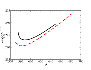
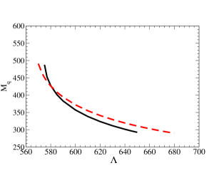
noting that the last equation remains unmodifed with respect to the LN case (except for the obvious replacement $M^{\rm LN}\to M^{\rm OPT}$). In both cases, $\langle\bar{q}q\rangle$ values are varied within a certain range of $\Lambda$ input values. Results are summarized in Figs. 3 and 4, for the quark condensate and mass gap, respectively, with particular values given in Table 1. The resulting values are roughly consistent with the allowed range from precise $\langle\bar{q}q\rangle$ determinations, in particular recent ones from lattice calculations qqlatt or spectral sum rules qqSR . Although the lattice determinations in particular have considerably restricted the allowed $\langle\bar{q}q\rangle$ value recently, they still allow rather conservative range of variation of $\langle\bar{q}q\rangle$ because of the relatively large systematic uncertainties.

As one can see, the mass gap and the quark condensate are quite sensitive to the value of the cutoff, especially for the mass gap, as expected, when it approaches a range where $M_{q}/\Lambda$ is no longer small. Note that there exist minimal values of $\Lambda$ (or alternatively minimal values of $-\langle\bar{q}q\rangle$) to obtain a self-consistent solution to all relevant quantities. This is similar in the LN case, except that those “theoretical” lower and upper bounds are somewhat more restrictive in the OPT case. The lower bounds are, in the OPT case, approximately $\Lambda\sim 575$ MeV, and $-\langle\bar{q}q\rangle\sim(242{\rm MeV})^{3}$, as is clear from the figures, thus producing the considered range of $\Lambda$ and $\langle\bar{q}q\rangle$. The LN approximation allows a rather similar lower value of $-\langle\bar{q}q\rangle\sim(240{\rm MeV})^{3}$, but for a lower minimal value of $\Lambda$ buballa . Therefore, the consistency with the OPT expressions restricts more the possible $\langle\bar{q}q\rangle$ range than in the LN case, since we only obtain solutions in the range $242{\rm MeV}\raisebox{-3.69899pt}{~{}\shortstack{$<$ \\ [-0.07cm] $\sim$}}~{}-\langle\bar{q}q\rangle^{1/3}\raisebox{-3.69899pt}{~{}\shortstack{$<$ \\ [-0.07cm] $\sim$}}~{}250$ MeV. Note also that, for relatively low values of $\langle\bar{q}q\rangle$, there are twofold solutions of $\Lambda$ for $\langle\bar{q}q\rangle$ input, as is clear from the figure: This is inherent to the structure of the determining equations. It is easy to get rid of one of the branch solutions by excluding unacceptably large values of $M_{q}$ (which on one of the branches, not shown on Fig. 4, grows very rapidly as a function of $\Lambda$, with $M_{q}>500$ MeV). Thus we only consider the branch with reasonable values of the constituent quark mass, as shown in Fig. 4.

Figure 3: (color online) Quark condensate as function of $\Lambda$ for $T=0$. The OPT is represented by the continuous line and the LN approximation by the dashed line. Both quantities are in MeV units.

Figure 4: (color online) Effective quark mass gap as a function of $\Lambda$ for $T=0$. The OPT is represented by the continuous line and the LN approximation by the dashed line. Both quantities are in MeV units.

Table 1: Basic parameters $G$, $m_{c}$ values and comparison of $M_{q}$, $\langle\bar{q}q\rangle$ predictions from fitting input data $m_{\pi}=135$ MeV; $f_{\pi}=92.4$ MeV: a) as function of cutoff $\Lambda$; b) fitting $\Lambda$ from $\langle\bar{q}q\rangle$. All mass parameters are in MeV units and the bag constant, ${\cal B}$, is given in ${\rm MeV}/{\rm fm}^{3}$.

$\Lambda$ input [MeV]	$G\Lambda^{2}$	$m_{c}$	$M_{q}$	$-\langle\bar{q}q\rangle^{1/3}$	$\frac{-2m_{c}\langle\bar{q}q\rangle}{f^{2}_{\pi}m^{2}_{\pi}}$	${\rm Re}[m_{\sigma}]$	${\cal B}$
(OPT-I) 580	2.46	5.0	427.7	243.6	0.93	911.5	199.11
(LN-I) 580	2.54	5.6	426.5	240.6	1.001	856	162.58
(OPT-II) 640	1.99	4.9	301.4	248	0.95	669	91.00
(LN-II) 640	2.14	5.2	319.5	247	1.00	644	87.90
$-\langle\bar{q}q\rangle^{1/3}$ input	$G\Lambda^{2}$	$m_{c}$	$M_{q}$	$\Lambda$	$\frac{-2m_{c}\langle\bar{q}q\rangle}{f^{2}_{\pi}m^{2}_{\pi}}$	$Re[m_{\sigma}]$	${\cal B}$
(OPT-III) 250	1.95	4.8	300	653	0.96	668	84.45
(LN-III) 250	2.08	5.0	303.5	659	1.00	680	78.88

One may remark at this stage that the corrections brought about by the OPT to the mass gap and quark condensate, for a given $\Lambda$, are rather moderate for the mass and even smaller for $\langle\bar{q}q\rangle$. These OPT corrections to LN can be a priori of any sign, depending on $\Lambda$ values, but with a tendency for the OPT mass gap to be slightly lower than the corresponding LN one, with a maximal departure of about $\sim 20$ MeV for $\Lambda\sim 630-640$ MeV. Indeed, it is worth mentioning that the bulk of OPT correction as compared with the LN result is coming from the very first term in the right-hand side of Eq. (45). In comparison, the ${\cal O}(G)$ two-loop correction gives a much more moderate effect, suppressed by a relative ${\cal M}^{2}/\Lambda^{2}$, making about 1 % of the total contribution to $f_{\pi}$ e.g. for parameter set II of Table 1. In fact, since ${\cal M}\simeq[1+1/(4N_{c})]M^{\rm OPT}_{q}\simeq 1.08M^{\rm OPT}_{q}$, from Eq. (24), as induced by the OPT “nonperturbative” corrections from Eq. (21), and replaces $M^{\rm LN}_{q}$ at first order in Eq. (45), one may have $M^{\rm OPT}_{q}<M^{\rm LN}_{q}$ from fitting the precise value of $f_{\pi}$ with Eq. (45).

Then, from the OPT expressions of $f_{\pi}$, $m_{\pi}$ and $\langle\bar{q}q\rangle$, one quantity of interest which is straightforward to determine within the OPT is the Gell–Mann-Oakes-Renner (GMOR) relation gmor : The latter can be conveniently defined as

$$R_{\rm GMOR}\equiv-2m_{c}\frac{\langle\bar{q}q\rangle}{f^{2}_{\pi}\,m^{2}_{\pi}}\;,$$ (50)

where $R^{\rm LN}_{\rm GMOR}\simeq 1$ in LN, up to tiny ${\cal O}(m^{2}_{c}/M^{2})$ corrections. The “exact” values of the OPT corrections $R^{\rm OPT}_{\rm GMOR}$ for a given $\Lambda$ are immediately obtained from the fitted values of $m_{c}$, and $\langle\bar{q}q\rangle$ and are given in Table 1. It may be useful, in addition, to give an approximate expression by combining the expressions for $f_{\pi}$, $m_{\pi}$, and $\langle\bar{q}q\rangle$, given, respectively, in Eqs. (45), (48) and (49): Expanding those relations to first order in $G$, neglecting the small $q^{2}$ dependence inside the $I_{4}(q^{2})$ integral (i.e. assuming $I_{4}(m^{2}_{\pi})\simeq I_{4}(0)$), and finally neglecting the tiny ${\cal O}(m^{2}_{c}/M^{2})$ corrections, we obtain:

$$R^{\rm OPT}_{\rm GMOR}\simeq\left(1+\frac{1}{4N_{c}}\right)^{-2}\>\left\{1+4\,G\left[I_{2}(0,0)-5{\cal M}^{2}I_{4}(0)+\frac{m^{2}_{\pi}}{2}I_{4}(0)\right]\right\}\;.$$ (51)

Again, we remark that a large part of the correction with respect to LN comes about simply from the factor $(1+1/(4N_{c}))^{-2}\sim 0.85$ induced by the specific nonperturbative OPT relation in Eq. (24), although this is partly compensated by the (positive) ${\cal O}(G)$ corrections (formally of order $1/N_{c}$ since $G\sim 1/N_{c}$) inside the bracket of Eq. (51) (which is about $10\%$ for the relevant values of the parameters), so that the final OPT (negative) corrections in Table 1 are not more than a few percent.
It is instructive to compare at this stage those results with the present theoretical status and constraints on the GMOR relation. As is well-known, the latter corresponds to the leading term in the expansion in powers of the quark masses. Theoretically, Chiral Perturbation Theory (ChPT) chpt typically predicts, at next-to-leading orders leutwyler1 , a few percent decrease from $R^{\rm GMOR}=1$, and even somewhat larger deviations have been advocated descotes1 in a generalized ChPT framework (where contributions of different ChPT orders could compete). Experimentally, one can extract indirectly the GMOR relation (or equivalently the value of the relevant ChPT parameters) from measurements of the $\pi\pi$ $S$-wave scattering lengths in $K\to\pi\pi l\nu$ scattering pipidata , upon additional theoretical assumptions and experimental information (see e.g. descotes1 ; descotes2 for a discussion). The latest precise measurement of the relevant S-wave scattering lengths NA48 , together with the most recent analysis performed in the framework of two-loop chiral perturbation theory, are consistent with a value $R^{\rm GMOR}\sim 0.94$ leutwyler1 ; leutwyler2 with a few percent accuracy. Thus, although considering the simplest $SU(2)$-symmetric NJL model can hardly compete with the latest sophistication level of ChPT to describe a fully realistic phenomenology, it is quite satisfactory at least that the OPT corrections we obtain appears roughly consistent with present constraints.

Another quantity of interest, at $T=0$ and $\mu=0$, is the “bag constant”, defined in terms of the pressure as buballa

$${\cal B}=P(M_{q})-P(m_{c})\,\,.$$ (52)

As shown in Tab. 1, this quantity is very sensitive to the parameter set used and ranges from $84.45{\rm MeV}/{\rm fm}^{3}$ to $199.11{\rm MeV}/{\rm fm}^{3}$ within the OPT and from $78.88{\rm MeV}/{\rm fm}^{3}$ to $162.58{\rm MeV}/{\rm fm}^{3}$ within the LN approximation

Finally, for completeness we evaluate the OPT expression for the $\sigma$ meson mass (at $T=\mu=0$) as usual by a procedure very similar to the one for the pion mass above, where the two-point function is that for a scalar, i.e., with $i\gamma_{5}\tau_{i}$ replaced by $1$ in both flavor and Dirac spaces within, e.g., Eq. (75) in Appendix B. At the one-loop level, the geometric resummation of this diagram produces a pole at $q^{2}=4M_{q}^{2}$ in the chiral limit, where $M_{q}$ is the mass gap. Evaluating all quantities including the OPT corrections induced at two-loop, and using the gap equation consistently at this order, gives a correction of ${\cal O}(G)$ to the well-known LN relation, and we are led to the final scalar meson mass given as the solution of the implicit equation

$$m^{2}_{\sigma} = 4(M^{\rm OPT}_{q})^{2}+\frac{m_{c}}{M^{\rm OPT}_{q}}\left(4GN_{\rm f}N_{c}I(m^{2}_{\sigma})\right)^{-1}$$ (53)

$$+ \frac{1}{4G\,I(m^{2}_{\sigma})}\left[i+8G\,I_{G}({\cal M})-i\>\sqrt{1-16iG\,I_{G}({\cal M})+64G^{2}\,I^{2}_{G}({\cal M})}\right]\;,$$

with $I(q^{2})$ as defined in Eq. (81). Note that actually, the OPT solution gives a relatively small correction to the one-loop relation $m^{2}_{\sigma}=4m^{2}+{\cal O}(m_{c})$, as can be seen more clearly by expansion of Eq. (53) to first order in $G$:

$$m^{2}_{\sigma}=4(M^{\rm OPT}_{q})^{2}+\frac{m_{c}}{M^{\rm OPT}_{q}}\left[4GN_{\rm f}N_{c}I(m^{2}_{\sigma})\right]^{-1}-16iG\frac{I^{2}_{G}({\cal M})}{I(m^{2}_{\sigma})}+{\cal O}(G^{2})\;.$$ (54)

Numerically, for the set II input values in Table 1, corresponding to $\Lambda=640$ MeV, we obtain: $m^{\rm OPT}_{\sigma}\simeq 669+17\,i$ MeV, to be compared with the corresponding LN value for the same input: $m^{\rm LN}_{\sigma}\simeq 644+0.8\,i$ MeV. Thus it gives a few percent correction to the standard (i.e LN) NJL result. Other values are given for illustration in Table 1. Thus the standard NJL picture at leading LN order predicting a sharp resonance, conflicting the very large $\sigma$ width, is not drastically modified by OPT first order corrections which basically use the same (variationally modified) NJL Lagrangian. Of course it would be possible in principle within OPT framework to evaluate the dominant $\sigma\to\pi\pi$ decay mode by calculating an effective $\sigma\pi\pi$ coupling, via a quark loop vertex graph with external $\pi$ and $\sigma$, thus providing some definite corrections to such similar LN approaches (which roughly gave the right order of magnitude of the $\sigma$ width (see e.g. njlrev3 and ref. therein)). However, already at LN order this raises a number of conceptual problems, and anyway such OPT corrections would certainly not accomodate all phenomenologically realistic properties of the $\sigma$ meson. As is well-known the $\sigma$ resonance had a long history with many controversies on its status, which is not yet fully clarified mesonrev . We therefore refrain to investigate more details on the $\sigma$ meson mass and other properties, which is well beyond the scope of the present work.

Before considering the model for non-zero temperature and chemical potential, it may be worth to review, at this stage, some definite differences betwen the OPT corrections obtained for the vacuum quantities and some other approaches beyond mean-field approximation, like typically the corrections obtained from the $1/N_{c}$ expansion nloNc ; oertel . Note that our OPT corrections beyond the LN/MFA results for all quantities ($M^{\rm OPT}$, $f_{\pi}$, $\langle\bar{q}q\rangle$, …) are formally organized to be of order ${\cal O}(1/N_{c}$, since $G\sim 1/N_{c}$ in a consistent $1/N_{c}$-expansion framework. However, as discussed in introduction, OPT differs in several respect from the genuine $1/N_{c}$ expansion, both qualitatively and quantitatively. More precisely, some relevant differences are as follows:

• As we already mentioned, at first OPT order the relevant two-loop calculations actually reduce to one-loop squared contributions, thus regularized by a single standard cutoff $\Lambda$, in contrast with the genuine $1/N_{c}$ corrections where an independent cutoff $\Lambda_{M}$ parameter is sometimes introduced to regularize the (meson) loops oertel .

• The mechanism satisfying the Goldstone theorem in OPT, via (perturbative) cancellations of different contributions, is somewhat similar to the one at work in the $1/N_{c}$ case nloNc , except that the latter involves extra $1/N_{c}$ contributions that are higher OPT orders (i.e. ${\cal O}(\delta^{2}G^{3})$), and therefore omitted in the OPT case. (Note that the consistency of OPT with the Goldstone theorem was also recently shown in the different context of the $O(N)$ $\phi^{4}$ model chhat .)

• in the $1/N_{c}$ framework one obtains a correction to the standard NJL (LN) $M_{q}$ versus $\langle\bar{q}q\rangle$ relation, Eq. (49), while the latter LN form is preserved at first OPT order (with simply the replacement $M_{q}^{\rm LN}\to M_{q}^{\rm OPT}$). This has another practical consequence concerning the GMOR relation, which receives only higher $1/N^{2}_{c}$ order corrections within the $1/N_{c}$ framework oertel , while OPT gives formally explicitly $1/N_{c}$ corrections, in Eq. (51) (though those are partially canceled by the extra ${\cal O}(G)\sim 1/N_{c}$ terms, as already discussed above).

We will consider each of the relevant cases as a function of the temperature and chemical potential. To compare OPT versus standard LN results, we will take as a representative case for input parameter values mainly those from set II from Table 1, corresponding to $\Lambda=640$ MeV, which gives reasonable values both for the quark mass and condensate. We have also studied the dependence of our main results upon varyiations of those input parameters within acceptable ranges, and will comment on this dependence when it is relevant.

VI Numerical results at finite temperature and density

Let us now turn to the study of the effects of temperature and chemical potential in the NJL model within the OPT starting with the finite-temperature and zero-chemical potential case.

VI.1 Hot matter at zero density

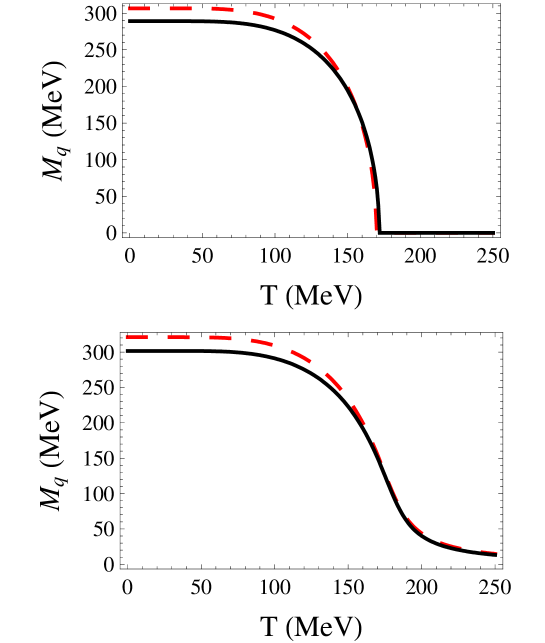
This scenario is important for observation the melting of the condensate, ${\bar{\sigma}}_{c}$, owing to the appearance of thermal effects. Theoretically, this case can be more easily exploited by use of lattice techniques because of the absence of the sign problem in the partition function at zero chemical potential. Since $\mu=0$, Eq. (21) still holds and the thermal mass is readily obtained from the solution of the gap equation,

$$M^{\rm OPT}_{q}(T) = m_{c}+{\bar{\sigma}}_{c}^{\rm OPT}=m_{c}+4GN_{\rm f}N_{c}\;{\cal M}I_{2}(\mu=0,T\neq 0)\Bigr{|}_{\bar{\eta}+m_{c}={\cal M}}\,,$$ (55)

which is solved numerically. The OPT results for Eq. (55) are compared with the LN results in Fig. 5 for the case of finite and vanishing current mass respectively. The OPT displays a second order phase transition taking place at $T_{c}\simeq 172\,{\rm MeV}$, while the LN result is just a bit smaller at $T_{c}\simeq 170\,{\rm MeV}$. It is useful to compare these results with recent next to leading order (NLO) corrections to the LN approximation obtained within the 2PI (or $\Phi$-derivable) functional formalism newbuballa . It is shown in that case that the NLO corrections decrease the critical temperature in the chiral case. This is in a sense expected, due to the effect of the inclusion of fluctuations. In the OPT the results depart little from the LN ones at finite temperature and zero density at this lowest order. However, as we will be seen below, the inclusion of finite density effects result in much more pronunced change of the critical quantities and overall behavior of the thermodynamical quantities as compared to the LN case. Also seen e.g. from Fig. 5, the OPT predicts a slight smaller crossover temperature as compared with the LN case, which is in agreement with the recent results obtained in newbuballa from NLO corrections obtained with the 2PI formalism.

Figure 5: (color online) Constituent quark mass as a function of $T$ for $\mu=0$ with $m_{c}=0$ (top) and for the case of nonzero $m_{c}$ (bottom): $m_{c}=4.9\rm MeV$ (OPT) and $m_{c}=5.2\rm MeV$ (LN). The continuous line represents the OPT result and the dashed line represents the LN approximation.

All basic thermodynamic quantities can be derived from the pressure $P$, obtained from the free energy density Eq. (12) using $P=-{\cal F}(\bar{\sigma})$, with $\bar{\sigma}$ obtained from the gap equation (19). It is also convenient to work directly in terms of the normalized pressure, $P_{N}(T,\mu)=P(T,\mu)-P(0,0)$ so that the energy density also vanishes at $T=0$ and $\mu=0$ (note that, although this subtraction at $T=0$ and $\mu=0$ is usual in the literature and it is done so to make contact with standard treatments in lattice calculations, it also removes some scale dependence). For simplicity we drop the subscript $N$ in all relations involving $P$ in the following.

In Figs. 6, 7, 8 and 9 we give as a function of the temperature, respectively, the interaction measure (or trace anomaly) $\Delta$, the conformal measure ${\cal C}$, the sound velocity squared $V_{s}^{2}$, and the equation of state parameter $w$. These quantities are defined, as usual, by the expressions,

$$\Delta=\frac{\epsilon-3P}{T^{4}}\;,$$ (56)

$${\cal C}=\frac{\Delta}{\epsilon}\simeq 1-3V_{s}^{2}\;,$$ (57)

$$V_{s}^{2}=\frac{dP}{d\epsilon}\;,$$ (58)

$$w=P/\epsilon\;.$$ (59)

Here the energy density, $\epsilon$, is defined as $\epsilon=-P+T\,s+\mu\,\rho$, where $s$ is the entropy density, $s=(\partial P/\partial T)_{\mu}$, and $\rho$ the quark number density, $\rho=(\partial P/\partial\mu)_{T}$. The interaction measure is useful to give the amount of scale violation through the different phases the system can have, while the conformal measure shows how the system might approach the ideal gas case, in which ${\cal C}=0$, or $V_{s}^{2}=1/3$. Both quantities are expected to peak near a phase transition or a crossover, thus being useful in locating the critical line. Because of our choice of regularization for the thermal integrals we expect that the OPT and LN will agree at high temperaures reproducing the Stefan-Boltzmann limit. This is shown in Figs. 6 and 7.

Figure 6: (color online) Interaction measure, $\Delta$, as a function of $T$ for $\mu=0$. The continuous line represents the OPT result and the dashed the LN approximation.

Figure 7: (color online) Conformal measure, ${\cal C}$, as a function of $T$ for $\mu=0$. The continuous line represents the OPT result and the dashed the LN approximation.

Figure 8: (color online) Sound velocity squared, $V_{s}^{2}$, as a function of $T$ for $\mu=0$. The continuous line represents the OPT results and the dashed the LN approximation.

Figure 9: (color online) Equation of state parameter, $w=P/\epsilon$, as a function of $T$ for $\mu=0$. The continuous line represents the OPT result and the dashed the LN approximation.

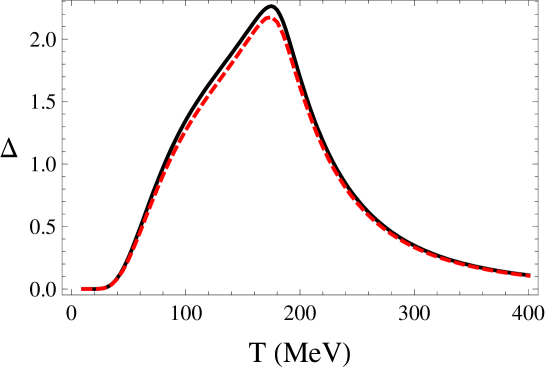
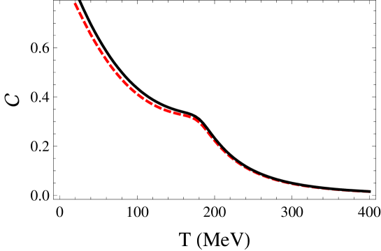
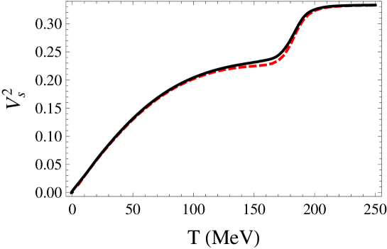
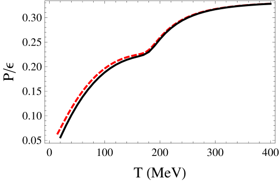
Figures 6, 7, 8 and 9 show the results for both the OPT and LN cases. We notice that the differences between the two approximations are small for all these quantities, thus indicating a robustness of the LN approximation when only thermal effects are considered. As expected all quantities have a smooth behavior around the temperature values where the crossover takes place. The OPT predicts a slightly higher interaction measure and speed of sound at the crossover.

VI.2 Cold matter at finite density

The effects caused by the OPT first-order corrections for cold and dense quark matter can now also be studied at $T=0$ and $\mu\neq 0$. Physically this situation is relevant in studies related to neutron stars for example. This is also the case where lattice techniques face more problems with the sign problem. As discussed before, in this case the simple PMS gap relation, Eq. (21), does not hold and we shall proceed numerically. Let us first define the integrals $I_{1}$, $I_{2}$ and $I_{3}$ in the limit $T\to 0$, with $\mu\neq 0$. They read

$$I_{0}(\mu,T=0)=\int\frac{d^{3}p}{\left(2\pi\right)^{3}}\theta(\mu-E_{p})=\frac{\theta(\mu-\eta-m_{c})}{6\pi^{2}}\left[\mu^{2}-(\eta+m_{c})^{2}\right]^{3/2}\;,$$ (60)

$$I_{1}(\mu,T=0)-I_{1}(0,0) = \int\frac{d^{3}p}{\left(2\pi\right)^{3}}(\mu-E_{p})\theta(\mu-E_{p})$$ (61)

$$= \frac{\theta(\mu-\eta-m_{c})}{32\pi^{2}}\left\{(\eta+m_{c})^{4}\ln\left[\frac{\left(\sqrt{\mu^{2}-(\eta+m_{c})^{2}}\mathbf{+}\mu\right)^{2}}{(\eta+m_{c})^{2}}\right]\right.$$

$$+ \left.\frac{10}{3}\mu\left[\mu^{2}-(\eta+m_{c})^{2}\right]^{\frac{3}{2}}{-2\mu^{3}}\sqrt{{\mu^{2}-(\eta+m_{c})^{2}}}\right\}\;,$$

and

$$I_{2}(\mu,T=0)-I_{2}(0,0) = -\int\frac{d^{3}p}{\left(2\pi\right)^{3}}\frac{1}{E_{p}}\theta(\mu-E_{p})$$ (62)

$$= -\frac{\theta(\mu-\eta-m_{c})}{4\pi^{2}}\left\{\mu\sqrt{\mu{{{}^{2}}\mathbf{-}(\eta+m_{c})^{2}}}-\frac{(\eta+m_{c})^{2}}{2}{\ln}\left[\frac{\left(\mu\mathbf{+}\sqrt{\mu{{{}^{2}}\mathbf{-}(\eta+m_{c})^{2}}}\right)^{2}}{(\eta+m_{c})^{2}}\right]\right\}\;,$$

where $I_{1}(0,0)$ and $I_{2}(0,0)$ are given by Eqs. (16) and (17), respectively. Next, the mass is obtained by considering

$$M^{\rm OPT}_{q}(\mu)=m_{c}+4GN_{\rm f}N_{c}(\bar{\eta}+m_{c})I_{2}(\mu,T=0)\,\,,$$ (63)

where the optimum, ${\bar{\eta}}$ is determined numerically upon solving the implicit equation,

$$\left\{\left[\eta-4G(\eta+m_{c}){\cal G}(N)I_{2}\right]\left[1+(\eta+m_{c})\frac{d}{d\eta}\right]I_{2}+4GI_{3}\frac{d}{d\eta}I_{3}\right\}_{\eta={\bar{\eta}}}=0\,\,,$$ (64)

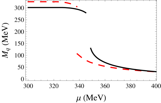
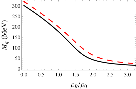
which is obtained by substitution of Eq. (19) in Eq. (18). Note that this relation is valid only when one is interested in the minimum of the free energy, as for example when evaluating the pressure. Otherwise, Eq. (18), has to be used. Figure 10 shows the quark effective mass as a function of $\mu$, obtained with the OPT and the LN. The qualitative behavior is the same and the critical values for the first order phase transition are $\mu_{c}\simeq 348.83\,{\rm MeV}$ for the OPT and $\mu_{c}\simeq 338.32\,{\rm MeV}$ for the LN approximation.

Figure 10: (color online) Effective quark mass, in units of the vacuum mass, as a function of $\mu$ for $T=0$. The OPT is represented by the continuous line and the LN approximation by the dashed line.

Once the free energy is evaluated and its minimum is located, one can obtain the pressure using $P=-{\cal F}(\bar{\sigma})$. The density $\rho$ can now be easily computed by using $dP/d\mu$ and taking into account the gap and PMS equations. This gives

$$\rho=2N_{f}N_{c}I_{1}^{\prime}-2N_{f}N_{c}(m_{c}+{\bar{\eta}})({\bar{\eta}}-{\bar{\sigma}_{c}})I_{2}^{\prime}-8GN_{f}N_{c}I_{3}I_{3}^{\prime}+4GN_{f}N_{c}(m_{c}+{\bar{\eta}})^{2}I_{2}I_{2}^{\prime}\,,$$ (65)

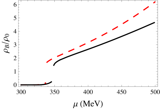
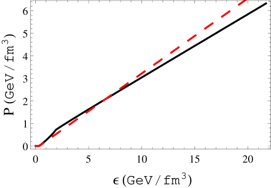
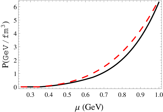
where the primes indicate derivatives with respect to $\mu$. Figure 11 shows the baryonic density $\rho_{B}=\rho/3$, in units of normal matter density ($\rho_{0}=0.17\,{\rm fm}^{-3}$), as a function of $\mu$. At $T=0$, the energy density is given as usual by $\epsilon=-P+\mu\rho$ and allows us to obtain the EoS as shown in Fig. 12 where the OPT appears to generate a softer relation due to a more abrupt change of slope at $\mu_{c}$.

Figure 11: (color online) Baryonic density, in units of $\rho_{0}=0.17\,{\rm fm}^{-3}$, as a function of $\mu$ for $T=0$. The continuous line corresponds to OPT and the dashed line to the LN approximation.

Figure 12: (color online) Equation of state generated by the OPT (continuous line) and the LN approximation (dashed line).

Figure 13: (color online) The pressure as a function of $\mu$ within the OPT (continuous line) and within the LN approximation (dashed line).

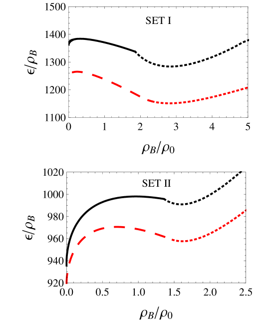
We now look at the matter stability by considering the energy per baryon number, $\epsilon/\rho_{B}=-P/\rho_{B}+3\mu$, as a function of the baryonic density, $\rho_{B}$. As Koch et al. koch found out, the NJL does not present a minimum at nuclear matter density, $\rho_{0}=0.17\,{\rm fm}^{-3}$. The situation can be remedied by introducing a vector coupling (see Refs buballa_stab ; koch for details). However, in the minimal form of the NJL considered in the present work one expects that stable matter can only occur in the chiral restored phase buballa_stab . Plots of the OPT quark effective mass in the chiral limit and away from it as functions of $\rho_{B}$ are shown in Fig. 14. The energy per baryon number as a function of the baryonic density is shown in Fig. 15, for both the OPT and LN cases with two sets of parameters in the chiral limit to illustrate how the energetically favored point changes from $\rho_{B}=0$, within set II, to $\rho_{B}\simeq 2.5\rho_{0}$, within set I, giving rise to stable matter.

Figure 14: The OPT quark effective mass as a function of the density for $m_{c}=4.9$ MeV (continuous) and $m_{c}=0$ (dot-dashed).

Figure 15: (color online) Energy per baryon number as a function of the baryonic density, in the chiral limit, for sets I and II as indicated in the figure. For the massive solutions, the OPT result is represented by the continuous line and the LN by the dashed line. The dotted lines represent the massless solutions in both cases.

Note that corrections beyond the LN approximation are more significant at finite density and $T=0$ than vice versa, as shown from Figs. 10-15. This points to the importance of the effect of fluctuations when studying dense matter. The same is true when considering the effects of both temperature and chemical potential, as we are going to analyze in the next subsection. Before doing that let us see how the critical temperature, $T_{c}(\mu=0)$, and the critical chemical potential, $\mu_{c}(T=0)$, change with the different sets of paramters. Here the quantity $T_{c}(\mu=0)$ can be defined only in the chiral limit ($m_{c}=0$) when a second order phase transition occurs for both approximations and any set of parameters. Away from the chiral limit a cross over takes place at $\mu=0$. On the other hand $\mu_{c}(T=0)$ can be defined for $m_{c}=0$ and $m_{c}\neq 0$ and in the first case a first order transition occurs for both approximations and any set of parameters. However, when set III is considered at $m_{c}\neq 0$ the LN predicts a very weak first order transition with a small latent heat while the OPT predicts a cross over also at $T=0$ (and everywhere in the $T-\mu$ plane). As emphasized in Ref. klevansky this is a possible scenario within the NJL where the order of the phase transition is indeed very sensitive to input parameters. In this respect our sets I and II seem to be more in lign with what one expects to happen in more realistic situations. Table 2 summarizes the numerical results for these critical quantities when the three parameter sets are employed by the two approximations considered here.

Table 2: Critical temperature at zero chemical potential, $T_{c}$, and critical chemical potential at zero temperature, $\mu_{c}$. Both quantities and the mass parameters are given in MeV. $T_{c}$ is evaluated at $m_{c}=0$ and $\mu_{c}$ at $m_{c}=0$ as well as at $m_{c}\neq 0$. For reference, the vacuum effective mass ($M_{q}$) evaluated at $m_{c}\neq 0$ is also shown.

$\Lambda$ input [MeV]	$G\Lambda^{2}$	$m_{c}$	$M_{q}$	$T_{c}(m_{c}=0)$	$\mu_{c}(m_{c}=0)$	$\mu_{c}(m_{c}\neq 0)$
(OPT-I) 580.0	2.5	5.0	427.7	198.0	428.0	439.6
(LN-I) 580.0	2.5	5.6	426.5	190.0	383.7	396.2
(OPT-II) 640.0	2.0	4.9	301.4	172.0	330.9	348.8
(LN-II) 640.0	2.1	5.2	319.5	170.0	319.4	338.3
$-\langle\bar{q}q\rangle^{1/3}$ input	$G\Lambda^{2}$	$m_{c}$	$M_{q}$	$T_{c}(m_{c}=0)$	$\mu_{c}(m_{c}=0)$	$\mu_{c}(m_{c}\neq 0)$
(OPT-III) 250.0	1.9	4.8	300.0	169.0	308.9	cross over
(LN-III) 250.0	2.1	5.0	303.5	167.0	323.0	329.0

VI.3 The Phase Diagram and the Critical End Point

We now consider the effects of both temperature and chemical potential in the thermodynamics of the NJL model. We start by first showing the results for the phase diagram in the $T-\mu$ plane, obtained from both the OPT and the LN approximations. Away from the chiral limit one expects to have a first order transition line starting at $T=0$ and at a finite $\mu$, whose value is of the order of the vacuum quark effective mass, $M_{q}$. This line vanishes at a critical end point (CEP) located at ($\mu_{E},T_{E}$). Then, for $\mu<\mu_{E}$ and $T>T_{E}$ a crossover occurs for finite $m_{c}$ values. Figure 16 displays the LN and OPT results, illustrating the situation. The OPT critical end point occurs at $T_{E}\simeq 22\rm{\rm MeV}$ and $\mu_{E}\simeq 345\rm{\rm MeV}$, while the LN approximation prediction is $T_{E}\simeq 37\rm{\rm MeV}$ and $\mu_{E}\simeq 326\rm{\rm MeV}$ (note that previous results for the critical end points in the NJL model at LN have also been calculated in e.g. Refs. barducci ).

Figure 16: (color online) Phase diagram in the $T-\mu$ plane. The continuous (OPT) and dashed (LN) lines refer to first order transition lines terminating at the CEP which are denoted by the dots.

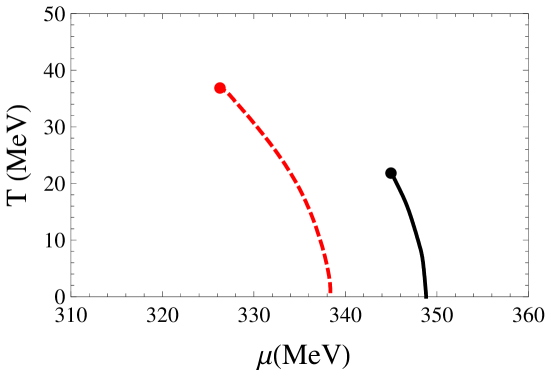
From Fig. 16 we can see that fluctuations brought about by considering corrections beyond the simple LN approximation can produce quite large corrections to the critical end points. $T_{E}$ is about $40\%$ smaller in the OPT case when compared to the LN, while $\mu_{E}$ is about $6\%$ higher in the OPT case. The crossover region is then larger in the OPT case when compared to the LN results.

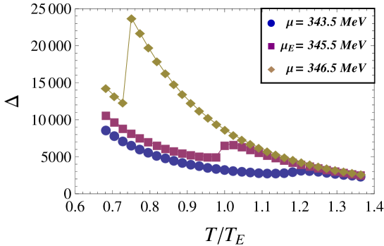
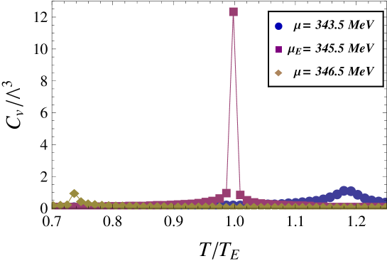
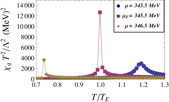
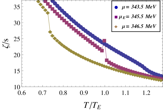
We next investigate the usefulness of the specific heat, the quark susceptibility and the bulk viscosity, as defined e.g. in karsch , as indicators of the location of the CEP since they all should peak at this point. We shall also see how discontinuities arise along the first order transition line within the interaction measure as defined by Eq. (56). The specific heat is given by its standard thermodynamic definition,

$$C_{v}=T\frac{\partial s}{\partial T}\;.$$ (66)

The quark susceptibility can be defined as

$$\chi_{q}=\ \frac{\partial\rho}{\partial\mu}\;.$$ (67)

The bulk viscosity is an intrinsic dynamical quantity. However, as shown in karsch , by use of a low-energy theorem of QCD, and assuming some reasonable ansatz for the spectral function, it was found that that bulk viscosity can be expressed in terms of the static thermodynamical quantities derived from the free energy as karsch

$$\zeta=\frac{1}{9\omega_{0}}\left[T^{5}\frac{\partial}{\partial T}\frac{(\epsilon-3P)}{T^{4}}+16|\epsilon_{0}|\right]\;,$$ (68)

where $\omega_{0}$ is a scale where perturbation theory becomes valid and that here we set it as the cutoff $\Lambda$ while $\epsilon_{0}$ is the vacuum part of the energy density.

In Fig. 17 we show the interaction measure as a function of the temperature at $\mu_{\rm CEP}$ and at values around $\mu_{\rm CEP}$. The same is shown in Figs. 18, 19 and 20, for the specific heat, the quark susceptibility and the ratio of the bulk viscosity to the entropy density. In all figures we notice the singular behavior around the CEP and is much more pronounced for the specific heat and the quark susceptibility. We can also see additional structure in all the plots for values of parameters away from the CEP showing a smooth behavoir for $T>T_{E}$ (crossover region) and a discontinuity at smaller temperatures (first-order transitions). In its standard definition the interaction measure is normalized by $T^{4}$ and therefore the discontinuities are greatly amplified for the $T<T_{E}$ situation. This is, for example, the case shown in Figs. 17 and 20 for $\mu=346.5$ MeV (but still smaller that $\mu_{E}$), where the discontinuity happens at the value of the temperature crossing the critical line shown in Fig. 16.

Figure 17: (color online) OPT results for the interaction measure, $\Delta$, as a function of $T/T_{E}$ where $T_{E}$ is the CEP temperature in the OPT case. The lines represent situations for $\mu<\mu_{E}$, $\mu=\mu_{E}$ and $\mu>\mu_{E}$ where $\mu_{E}$ is the CEP in the OPT case.

Figure 18: (color online) OPT results for the dimensionless specific heat, $C_{v}/\Lambda^{3}$, as a function of $T/T_{E}$ where $T_{E}$ is the CEP temperature in the OPT case. The lines represent situations for $\mu<\mu_{E}$, $\mu=\mu_{E}$ and $\mu>\mu_{E}$ where $\mu_{E}$ is the CEP in the OPT case.

Figure 19: (color online) OPT results for the normalized quark susceptibility, $\chi_{q}(T/\Lambda)^{2}$, as a function of $T/T_{E}$ where $T_{E}$ is the CEP temperature in the OPT case. The lines represent situations for $\mu<\mu_{E}$, $\mu=\mu_{E}$ and $\mu>\mu_{E}$ where $\mu_{E}$ is the CEP in the OPT case.

Figure 20: (color online) OPT results for the bulk viscosity over entropy density, $\zeta/s$, as a function of $T/T_{E}$ where $T_{E}$ is the CEP temperature in the OPT case. The lines represent situations for $\mu<\mu_{E}$, $\mu=\mu_{E}$ and $\mu>\mu_{E}$ where $\mu_{E}$ is the CEP in the OPT case.

VII Conclusions

We have used the OPT nonperturbative approximation to evaluate Landau’s free energy density for the $SU(2)$ version of the NJL model. By adopting an adequate form for the interpolation mass parameter we have shown that, in the large-$N_{c}$ limit, the LN (or MFA) result is exactly reproduced. At the first non-trival OPT order, which incorporates a large part of $1/N_{c}$ corrections but does not involve new parameters beyond those of the LN model, we have established the consistency with the Goldstone theorem. We have derived a consistent set of input parameters by matching the model with OPT corrections to the pion mass and decay constant experimental values, and obtained consequently OPT deviations from leading-order results in some quantities, such as typically the GMOR relation. We then analyzed the cases of zero temperature and chemical potential, finite temperature and zero chemical potential, zero temperature and finite chemical potential and for both nonzero temperature and chemical potential. In each of these cases we have compared the results for the LN approximation with those from the OPT.

For the finite-temperature, but zero-chemical potential cases, we have seen that the inclusion of higher-order corrections to the LN case changes the LN results only slightly, with changes being at most at about $7\%$. No change of qualitative behavior is observed and our results then support the robustness of the LN approximation in the studies of the 3+1 dimensional NJL when only thermal effects are concerned. However, the inclusion of density effects produce results that can lead to a much higher difference between the LN and when fluctuations are taken into account. This is the case, for example, seen in determination of the CEP in the phase diagram of the NJL model at finite temperature and density. The situation could be antecipated if we recall that, at first order, the $1/N_{c}$ corrections considered by the OPT are basically given by the square of the scalar density ($\langle{\bar{\psi}}\psi\rangle^{2}$) as well as the square of the quark number density ($\langle{\psi}^{+}\psi\rangle^{2}$). Because of the Dirac algebra matrices, contributions from the scalar and pseudoscalar channels partially cancel in the former while they add up for the latter. This is interesting since then the OPT can be considered a good alternative to the LN approximation in regimes where lattice evaluations become more delicate.

The study of the application of the OPT method to the thermodynamics of the NJL model made here can also be readily extented to the Polyakov-loop case of the NJL model. In this case we expect to improve the many thermodynamical studies made in this context (see e.g. wambach ; kenji ; chineses for recent references). We will be reporting on these results elsewhere.

Finally, we have analyzed quantities like the interaction measure (or trace anomaly), the specific heat, the quark susceptibility and the bulk viscosity as possible indicators for locating the CEP of QCD, showing that these important points can be located through singular behavior of these functions, which is more pronounced for the cases of the specific heat and the quark susceptibility.

Appendix A Summing Matsubara frequencies and related formulas

In this appendix we give the results for the main integrals and Matsubara sums appearing along the text. The Matsubara sums which are relevant for the different integrals considered in our work can be derived as (see e.g. kapusta )

$$T\sum_{n=-\infty}^{+\infty}\ln[(\omega_{n}-i\mu)^{2}+E_{p}^{2}]=E_{p}+T\ln\left[1+e^{-\left(E_{p}+\mu\right)/T}\right]+T\ln\left[1+e^{-\left(E_{p}-\mu\right)/T}\right],$$ (69)

where $E_{p}^{2}=\mathbf{p}^{2}+\eta^{2}$. The zero temperature limit of Eq. (69) is given by

$$\lim_{T\rightarrow 0}T\sum_{n=-\infty}^{+\infty}\ln[(\omega_{n}-i\mu)^{2}+E_{p}^{2}]=E_{p}+\left(\mu-E_{p}\right)\theta(\mu-E_{p})=\mathrm{max}(E_{p},\mu)\;.$$ (70)

Likewise, the term,

$$T\sum_{n=-\infty}^{+\infty}\frac{1}{(\omega_{n}-i\mu)^{2}+E_{p}^{2}}=\frac{1}{2E_{p}}\left[1-\frac{1}{e^{\left(E_{p}+\mu\right)/T}+1}-\frac{1}{e^{\left(E_{p}-\mu\right)/T}+1}\right],$$ (71)

gives

$$\lim_{T\rightarrow 0}T\sum_{n=-\infty}^{+\infty}\frac{1}{(\omega_{n}-i\mu)^{2}+E_{p}^{2}}=\frac{1}{2E_{p}}\left[1-\theta(\mu-E_{p})\right];$$ (72)

Finally, the finite temperature and density expression

$$T\sum_{n=-\infty}^{+\infty}\frac{\omega_{n}-i\mu}{(\omega_{n}-i\mu)^{2}+E_{p}^{2}}=\frac{i}{2}\left[\frac{1}{e^{\left(E_{p}-\mu\right)/T}+1}-\frac{1}{e^{\left(E_{p}+\mu\right)/T}+1}\right]\;,$$ (73)

gives, as $T\rightarrow 0$,

$$\underset{T\rightarrow 0}{\lim}T\sum_{n=-\infty}^{+\infty}\frac{\omega_{n}-i\mu}{(\omega_{n}-i\mu)^{2}+E_{p}^{2}}=\frac{i}{2}{\rm sgn}\left(\mu\right)\theta(\mu-E_{p})\;.$$ (74)

Appendix B Two-loop calculations for $m_{\pi}$ and $f_{\pi}$

We consider the (first) vertex correction graph to the pion self-energy in Fig. 2 which is not incorporated by OPT mass insertions within the one-loop contributions. Calling its contribution $\Pi^{(2),ps}_{\pi\>ij}(q^{2})$ for the pseudoscalar exchange graphs with integration momenta $p_{1},p_{2}$ and external momentum $q$, one obtains in Minkowski space:

$$-i\Pi^{(2),ps}_{\pi\>ij}(q^{2})=i\frac{\lambda}{2}\int\frac{d^{4}p_{1}}{(2\pi)^{4}}\frac{d^{4}p_{1}}{(2\pi)^{4}}\>Tr[(i\tau_{k}\gamma_{5})\frac{i}{p_{1}{\hbox{$\!\!\!\!\!/$}}-m}(i\tau_{i}\gamma_{5})\frac{i}{p_{1}{\hbox{$\!\!\!\!\!/$}}+q{\hbox{$\!\!\!/$}}-m}(i\tau_{k}\gamma_{5})\frac{i}{p_{2}{\hbox{$\!\!\!\!\!/$}}+q{\hbox{$\!\!\!/$}}-m}(i\tau_{j}\gamma_{5})\frac{i}{p_{2}{\hbox{$\!\!\!\!\!/$}}-m}]\;,$$ (75)

while the diagram with scalar $\sigma$ exchange is given by the same expression with $i\tau_{k,l}\gamma_{5}\to 1$ replacements in flavor and Dirac space. (Note thus that the $\sigma$-exchange graph has a relative minus sign with respect to the pion exchange, apart from any other possible factors). After taking the trace in color, flavor and Dirac spaces, using $\mbox{Tr}\>\tau_{i}\tau_{j}=2\delta_{ij}$, we obtain

$$\Pi^{(2),ps}_{\pi}(q^{2})= -4n_{\pi}\,N_{\rm f}\lambda\int\frac{d^{4}p_{1}}{(2\pi)^{4}}\frac{d^{4}p_{1}}{(2\pi)^{4}}F[p_{1}]F[p_{2}]\times$$

$$\left[p_{1}.(p_{1}+q)p_{2}.(p_{2}+q)-m^{2}[p_{1}.(p_{1}+q)+p_{2}.(p_{2}+q)]-m^{2}(q^{2}-m^{2})\right]\;,$$

where

$$F[p_{i}]=(p^{2}_{i}-m^{2})^{-1}[(p_{i}+q)^{2}-m^{2})]^{-1}\;.$$ (77)

Using then some standard relations like

$$\frac{p.(p+q)}{(p^{2}-m^{2})[(p+q)^{2}-m^{2}]}=\frac{1}{2}\left[\frac{1}{p^{2}-m^{2}}+\frac{1}{(p+q)^{2}-m^{2}}\right]+(m^{2}-\frac{q^{2}}{2})\frac{1}{[(p^{2}-m^{2})[(p+q)^{2}-m^{2}]}\;,$$ (78)

and upon shift of integration momenta Eq. (B) takes, after some algebra, the form

$$\Pi^{(2),ps}_{\pi}(q^{2})=-8GN_{f}N_{c}n_{\pi}\,\left[I^{2}_{G}(m)-q^{2}\left(I_{G}(m)I(q^{2})+m^{2}I^{2}(q^{2})-\frac{q^{2}}{4}I^{2}(q^{2})\right)\right]\;,$$ (79)

where we defined

$$I_{G}(m)=\int\frac{d^{4}p}{(2\pi)^{4}}\;\frac{1}{p^{2}-m^{2}}\;,$$ (80)

which is the standard integral relevant in the gap-equation, as well as

$$I(q^{2})=\int\frac{d^{4}p}{(2\pi)^{4}}\;\frac{1}{(p^{2}-m^{2})[(p+q)^{2}-m^{2}]}\;,$$ (81)

which is the standard integral appearing in the one-loop scalar pion self-energy contribution Eq. (28).
Calculation steps similar to those in Eqs. (B-79) give for the scalar $\sigma$ exchange two-loop graph contribution in Fig. 2):

$$\Pi^{(2),s}_{\pi}(q^{2})=8GN_{\rm f}N_{c}\,\left[I^{2}_{G}(m)-q^{2}\left(I_{G}(m)I(q^{2})-m^{2}I^{2}(q^{2})-\frac{q^{2}}{4}I^{2}(q^{2})\right)\right]\;.$$ (82)

Now combining the scalar and pseudoscalar contributions with the one-loop contribution (28), gives for the (inverse) resummed pion propagator the final expression

$$1-2G\,[\Pi^{(1)}(q^{2})+\Pi^{(2)}(q^{2})]=1-4iGN_{\rm f}N_{c}\>\left(2I_{G}(m)-q^{2}I(q^{2})\right)$$ (83)

$$+16G^{2}N_{\rm f}N_{c}\left[(n_{\pi}-1)\left[I^{2}_{G}(m)-q^{2}\left(I_{G}(m)\,I(q^{2})-\frac{q^{2}}{4}I^{2}(q^{2})\right)\right]-(n_{\pi}+1)q^{2}m^{2}I^{2}(q^{2})\right]\;.$$

By inserting the perturbative two-loop gap-equation Eq. (39) into the latter expression (in the chiral limit $m_{c}=0$) one obtains the expected Goldstone pole at $q^{2}=0$:

$$1-2G\,[\Pi^{(1)}(q^{2})+\Pi^{(2)}(q^{2})]=4GN_{\rm f}N_{c}\>q^{2}\left[i\,I(q^{2})-8G\left[I_{G}(m)\,I(q^{2})+\left(2m^{2}-\frac{q^{2}}{4}\right)I^{2}(q^{2})\right]\right]\;.$$ (84)

Finally, taking Eq. (B) with $m_{c}\neq 0$ and defining the pion mass as usual as the pole of this expression for $q^{2}=m^{2}_{\pi}$ gives the final relation defining $m_{\pi}$ at this OPT, Eq. (40).

By very similar calculations we can derive an expression for the two-loop vertex contribution to the $\sigma$-meson self-energy, relevant to calculate the $\sigma$ mass if needed. Contributions are given by graphs similar to those in Fig. 2 but with the replacement $i\gamma_{5}\tau_{i,j}\to 1$ in flavor and Dirac spaces. After some algebra, we obtain for the summed contribution of $\pi,\sigma$ exchanges the expression (at the moment for $m_{c}=0$):

$$\Pi^{(2),ps+s}_{\sigma}(q^{2})=8GN_{\rm f}N_{c}(n_{\pi}-1)\,\left[I^{2}_{G}(m)+(4m^{2}-q^{2})I_{G}(m)I(q^{2})+\frac{1}{4}\>(4m^{2}-q^{2})^{2}I^{2}(q^{2})\right]\;.$$ (85)

This expression has to be combined with the standard one-loop contribution:

$$\Pi^{(1)}_{\sigma}(q^{2})=4iGN_{\rm f}N_{c}\,\left[I_{G}(m)+\frac{1}{2}\>(4m^{2}-q^{2})I(q^{2})\right]\;,$$ (86)

to define the inverse resummed $\sigma$-meson propagator, with $m\to{\cal M}^{OPT}$ for consistency with the OPT order. Using the gap equation, and solving for the pole of this propagator gives a (quadratic) equation for $m^{2}_{\sigma}$, which explicit solution is given in Eq. (53).

We next discuss the two-loop contributions to the pion decay constant. Firstly, at one-loop order, one finds the well-known expression

$$if^{2}_{\pi}g_{\mu\nu}\delta^{ij}=-\frac{1}{4}\int\frac{d^{4}p}{(2\pi)^{4}}\>Tr[\frac{i}{p{\hbox{$\!\!\!/$}}-m}(i\tau_{i}\gamma_{\mu}\gamma_{5})\frac{i}{p{\hbox{$\!\!\!/$}}+q{\hbox{$\!\!\!/$}}-m}(i\tau_{j}\gamma_{\nu}\gamma_{5})]\;,$$ (87)

where the $1/4$ overall comes from $\tau_{i}/2$ normalization of axial currents and the overall minus takes into account trace over fermions. We adopt here as a covariant regularization dimensional regularization (at $D=4$) which is more convenient at two-loop order than Pauli-Villars. Then using $\mbox{Tr}\>\tau_{i}\tau_{j}=2\delta_{ij}$, and picking up the $g_{\mu\nu}$ coefficients after algebra gives for $q^{2}\to 0$

$$f^{2}_{\pi}(\mbox{1-loop})=-4iN_{c}m^{2}I(0)$$ (88)

which is fully consistent with the result obtainedklevansky from the alternative definition of $f_{\pi}$ via the one-pion to vacuum transition. At two-loop we have a vertex correction graph similar to the first graph in Fig. 2 but with the replacement: $i\gamma_{5}\tau_{i}\to i\gamma_{5}\gamma_{\mu}\tau_{i}/2$. One finds

$$if^{2}_{\pi}g_{\mu\nu}\delta^{ij}=i\frac{\lambda}{2}\int\frac{d^{4}p_{1}}{(2\pi)^{4}}\frac{d^{4}p_{1}}{(2\pi)^{4}}\>Tr[(i\tau_{k}\gamma_{5})\frac{i}{p_{1}{\hbox{$\!\!\!\!\!/$}}-m}(i\tau_{i}/2\gamma_{\mu}\gamma_{5})\frac{i}{p_{1}{\hbox{$\!\!\!\!\!/$}}+q{\hbox{$\!\!\!/$}}-m}(i\tau_{k}\gamma_{5})\frac{i}{p_{2}{\hbox{$\!\!\!\!\!/$}}+q{\hbox{$\!\!\!/$}}-m}(i\tau_{j}/2\gamma_{\nu}\gamma_{5})\frac{i}{p_{2}{\hbox{$\!\!\!\!\!/$}}-m}]\;.$$ (89)

By adopting again a Lorentz-covariant preserving regularization (we use dimensional regularization but for $D=4$), after some algebra we obtain the final result

$$f^{2}_{\pi}(\mbox{2-loop,vertex})=8GN_{c}(n_{\pi}-1)m^{4}I^{2}(0)\;,$$ (90)

where $I(q^{2})$ is the one-loop integral as defined in Eq. (81). The other remaining two diagrams in Fig. 2, of same order, will be again consistently obtained in our case via the OPT mass insertion within the one-loop $f_{\pi}$ expression, so that the final two-loop expression for $f_{\pi}$ is the one given in Eq. (44).

References

- (1) Y. Nambu and G. Jona-Lasinio, Phys. Rev. 122, 345 (1961); 124, 246 (1961).
- (2) S. P. Klevansky, Rev. Mod. Phys. 64, 649 (1992).
- (3) T. Hatsuda and T Kunihiro, Phys. Rept. 247 (1994) 221.
- (4) M. Buballa, Phys. Rep. 407, 205 (2005).
- (5) V. Dmitrasinovic, H.G. Schulze, R. Tegen and R. H. Lemmer, Ann. Phys. (NY) 238 332 (1995).
- (6) M. Oertel, M. Buballa and J. Wambach, Phys. Lett. B 477 77 (2000); M. Oertel, M. Buballa and J. Wambach, Yad. Fiz. 64 (2001) 757.
- (7) R. Seznec and J. Zinn-Justin, J. Math. Phys. 20, 1398 (1979); J. C. Le Guillou and J. Zinn-Justin, Ann. Phys. 147, 57 (1983); V. I. Yukalov, Moscow Univ. Phys. Bull. 31, 10 (1976); W. E. Caswell, Ann. Phys. (N.Y) 123, 153 (1979); I. G. Halliday and P. Suranyi, Phys. Lett. B85, 421 (1979); J. Killinbeck, J. Phys. A14, 1005 (1981); R. P. Feynman and H. Kleinert, Phys. Rev. A 34, 5080 (1986); H. F. Jones and M. Moshe, Phys. Lett. B234, 492 (1990); A. Neveu, Nucl. Phys. (Proc. Suppl.) B18, 242 (1990); V. Yukalov, J. Math. Phys 32, 1235 (1991); C. M. Bender et al., Phys. Rev. D45, 1248 (1992); H. Yamada, Z. Phys. C59, 67 (1993); A. N. Sissakian, I. L. Solovtsov and O. P. Solovtsova, Phys. Lett. B321, 381 (1994); C. Arvanitis, F. Geniet, M. Iacomi, J.-L. Kneur and A. Neveu, Int.J.Mod.Phys. A12, 3307 (1997); H. Kleinert, Phys. Rev. D 57, 2264 (1998); Phys. Lett. B434, 74 (1998); for a review, see H. Kleinert and V. Schulte-Frohlinde, Critical Properties of -Theories, Chap. 19 (World Scientific, Singapure 2001); K. G. Klimenko, Z. Phys. C50, 477 (1991); ibid. C60, 677 (1993); Mod. Phys. Lett. A9, 1767 (1994); M. B. Pinto, R. O. Ramos and P. J. Sena, Physica A342, 570 (2004).
- (8) J. Zinn-Justin, arXiv:1001.0675 [math-ph]
- (9) F. F. Souza Cruz, M. B. Pinto and R. O. Ramos, Phys. Rev. B 64, 014515 (2001); J.-L. Kneur, M. B. Pinto and R. O. Ramos, Phys. Rev. Lett. 89, 210403 (2002); Phys. Rev. A 68, 043615 (2003); E. Braaten and E. Radescu, Phys. Rev. Lett. 89, 271602 (2002), Phys. Rev. A 66, 063601 (2002); J.-L. Kneur, A. Neveu and M. B. Pinto, Phys. Rev. A 69, 053624 (2004); B. Kastening, Phys. Rev. A 70, 043621 (2004); J.-L. Kneur and M. B. Pinto, Phys. Rev. A 71, 033613 (2005).
- (10) M. B. Pinto and R. O. Ramos, Phys. Rev. D 60, 105005 (1999); ibid. 61, 125016 (2000); R. L. S. Farias, G. Krein and R. O. Ramos, Phys. Rev. D 78, 065046 (2008).
- (11) J.-L. Kneur, M. B. Pinto and R. O. Ramos, Phys. Rev. D 74, 125020 (2006).
- (12) J.-L. Kneur, M. B. Pinto, R. O. Ramos and E. Staudt, Phys. Rev. D 76, 045020 (2007); Phys. Lett. B567, 136 (2007).
- (13) E. S. Fraga, L. Palhares and M. B. Pinto, Phys. Rev. D 79, 065026 (2009)
- (14) H. Caldas, J.-L. Kneur, M. B. Pinto and R. O. Ramos, Phys. Rev. B 77, 205109 (2008).
- (15) J. B. Kogut and C. G. Strouthos, Phys. Rev. D 63, 054502 (2001).
- (16) J.-L. Kneur and A. Neveu, arXiv:1004.4834 (in press Phys. Rev. D).
- (17) M. C. B. Abdalla, J. A. Helayël-Neto, D. L. Nedel and C. R. Senise Jr., Phys. Rev. D 80, 065002 (2009).
- (18) C. Arvanitis, F. Geniet, J.-L. Kneur and A. Neveu, Phys. Lett. B 390, 385 (1997); J.-L. Kneur, Phys. Rev. D 57, 2785 (1998).
- (19) J. O. Andersen, E. Braaten and M. Strickland, Phys. Rev. Lett. 83, 2139 (1999); Phys. Rev. D 61, 014017 (2000); J. O. Andersen, M. Strickland, and N. Su, Phys. Rev. Lett. 104, 122003 (2010).
- (20) M. Buballa, Nucl. Phys. A 611, 393 (1996).
- (21) V. Koch, T. S. Biro, J. Kunz, and U. Mosel, Phys. Lett. B 185, 1 (1987).
- (22) O. A. Battistel, G. Dallabona, and G. Krein, Phys. Rev. D 77, 065025 (2007).
- (23) A. Okopinska, Phys. Rev. D 35, 1835 (1987); M. Moshe and A. Duncan, Phys. Lett. B215, 352 (1988).
- (24) S. K. Gandhi and M. B. Pinto. Phys. Rev. D 46, 2570 (1992).
- (25) P. M. Stevenson, Phys. Rev. D 23, 2961 (1981); Nucl. Phys. B 203, 472 (1982).
- (26) K. Fukushima, Phys. Lett. B591, 277 (2004).
- (27) See e.g. for a very recent result: H. Fukaya et al, Phys. Rev. Lett. 104, 122002 (2010).
- (28) See e.g. H.G. Dosch and S. Narison, Phys. Lett. B 417 (1998) 173; M. Jamin, Phys. Lett. B 538, 71 (2002).
- (29) M. Gell-Mann, R. J. Oakes and B. Renner, Phys. Rev. 175, 2195 (1968).
- (30) J. Gasser and H. Leutwyler, Ann. Phys. (N.Y.) 158, 142 (1984); Nucl. Phys. B250, 465 (1985).
- (31) G. Colangelo, J. Gasser and H. Leutwyler, Phys. Rev. Lett. 86, 5008 (2001).
- (32) S. Descotes-Genon, N.H. Fuchs, L. Girlanda and J. Stern, Eur. Phys. J. C 24, 469 (2002).
- (33) S. Pislak et al. [BNL-E865 Collaboration], Phys. Rev. Lett. 87, 221801 (2001). Phys. Rev. D 67, 072004 (2003).
- (34) S. Descotes-Genon, Eur. Phys. J. C 52, 141 (2007).
- (35) J.R. Batley et al., Eur. Phys. J. C54, 411 (2008).
- (36) See, e.g., H. Leutwyler, Proceedings of the QCD 08 International Conference, Montpellier, France, Nucl. Phys. B Proceedings Supplements 186, 338 (2009).
- (37) See e.g. E. Klempt and A. Zaitsev, Phys. Rept. 404, 1 (2007).
- (38) S. Chiku and T. Hatsuda, Phys. Rev. D 58, 076001 (1998).
- (39) D. Müller, M. Buballa and J. Wambach, Phys. Rev. D81, 094022 (2010).
- (40) A. Barducci, R. Casalbuoni, Giulio Pettini and L. Ravagli, Phys. Rev. D 69, 096004 (2004); J. O. Andersen and L. Kyllingstad, J. Phys. G37, 015003 (2009).
- (41) D. Kharzeev and K. Tuchin, J. High Energy Phys. 09, 093, (2008); F. Karsch, D. Kharzeev and K. Tuchin, Phys. Lett. B 663, 217 (2008).
- (42) B.-J. Schaefer, J. M. Pawlowski and J. Wambach, Phys. Rev. D 76, 074023.
- (43) K. Fukushima, Phys. Rev. D 77, 114028 (2008).
- (44) H. Mao, J. Jin, and M. Huang, J. Phys. G 37, 035001 (2010).
- (45) J. I. Kapusta, Finite - Temperature Field Theory (Cambridge Universty Press, Cambridge, England, 1985); M. Le Bellac Thermal Field Theory (Cambridge Universty Press, Cambridge, England, 1996).