Bregman Distance to L1 Regularized Logistic Regression

Abstract

In this work we investigate the relationship between Bregman distances and regularized Logistic Regression model. We present a detailed study of Bregman Distance minimization, a family of generalized entropy measures associated with convex functions. We convert the L1-regularized logistic regression into this more general framework and propose a primal-dual method based algorithm for learning the parameters. We pose L1-regularized logistic regression into Bregman distance minimization and then apply non-linear constrained optimization techniques to estimate the parameters of the logistic model.

1 Introduction

We study the problem of regularized logistic regression as proposed by [5] and [12]. $L1$ regularization has been studied extensively during recent years due to the sparsity of the classifiers obtained by such regularization [11]. The objective function in the $L1$-regularized LRP (Eqn. 4) is convex, but not differentiable (specifically, when any of the weights is zero), so solving it is more of a computational challenge than solving the $L2$-regularized LRP. Despite the additional computational challenge posed by $L1$-regularized logistic regression, compared to $L2$-regularized logistic regression, interest in its use has been growing. The main motivation is that $L1$-regularized LR typically yields a sparse vector $\boldsymbol{\lambda}$, i.e., $\boldsymbol{\lambda}$ typically has relatively few nonzero coefficients. (In contrast, $L2$-regularized LR typically yields $\boldsymbol{\lambda}$ with all coefficients nonzero.) When ${\lambda}_{j}$ = 0, the associated logistic model does not use the jth component of the feature vector, so sparse $\boldsymbol{\lambda}$ corresponds to a logistic model that uses only a few of the features, i.e., components of the feature vector. Indeed, we can think of a sparse $\boldsymbol{\lambda}$ as a selection of the relevant or important features (i.e., those associated with nonzero ${\lambda}_{j}$), as well as the choice of the intercept value and weights (for the selected features). A logistic model with sparse $\boldsymbol{\lambda}$ is, in a sense, simpler or more parsimonious than one with non-sparse $\boldsymbol{\lambda}$. It is not surprising that $L1$-regularized LR can outperform $L2$-regularized LR, especially when the number of observations is smaller than the number of features.

Our work is based directly on the general setting of [12] in which one attempts to solve optimization problems based on general Bregman distances. They proposed the iterative scaling algorithm for minimizing such divergences through the use of auxiliary functions. Our work builds on several previous works which have compared divergence approaches to logistic regression. We closely follow the work by [5] who propose a new category of parallel and sequential algorithms for boosting and logistic regression based on Bregman distance minimization. They are one of the first to connect the fields of regression and generalized divergences, but as such unconstrained logistic parameter is unreliable for large problems and hence we take up this study to tie constrained optimization to the existing work.

Most of the work related to connecting the idea of Bregman distance and logistic regression minimize the unconstrained auxiliary function at each step. In this work we pose the problem with box or $L1$ constraints due to the favorable properties of $L1$ regularization for cases with large dimensions but relatively fewer number of training data points.

2 Logistic Regression

Let $\mathcal{S}=\langle(x_{1},y1),\dots,(x_{m},y_{m})\rangle$ be a set of training examples where each instance $x_{i}$ belongs to a domain or instance space $\boldsymbol{\chi}$ , and each label $y_{i}\in\{-1,+1\}$.

We assume that we are given a set of real-valued functions on $\boldsymbol{\chi}$, denoted by $h_{i}$ where $i=\{1,2,\dots,n\}$. Following convention in the Maximum-Entropy literature, we call these functions features; in the boosting literature, these would be called weak or base hypotheses. Note that, in the terminology of the latter literature, these features correspond to the entire space of base hypotheses rather than merely the base hypotheses that were previously found by the weak learner. We study the problem of approximating the $y_{i}$ s using a linear combination of features. That is, we are interested in the problem of finding a vector of parameters $\boldsymbol{\lambda}\in\mathbb{R}^{n}$ such that $f_{\lambda}(x_{i})=\sum_{j=1}^{n}\lambda_{j}h_{j}(x_{i})$ is a good approximation of $y_{i}$.

For classification problems, it is natural to try to match the sign of $f_{\boldsymbol{\lambda}}(x_{i})$ to $y_{i}$, that is, to attempt to minimize

$$\sum_{j=1}^{n}I_{\mathbb{[}y_{i}f_{\boldsymbol{\lambda}}(x_{i})\leq 0\mathbb{]}}$$ (1)

where $I_{\{c\}}=1$ whenever {c} is $true$. This form of loss is intractable for in its most general form and so some other non-negative loss function is minimized which closely resembles the above loss.

In the logistic regression framework we use the estimate

$$\mathrm{P}\{y=+1|x\}=\frac{1}{1+\exp(-f_{\boldsymbol{\lambda}}(x))}$$ (2)

and the log-loss for this model is defined as

$$\ell(\mathbf{x},\mathbf{y})=\sum_{j=1}^{m}\ln(1+exp(-y_{i}f_{\boldsymbol{\lambda}}(x_{i})))$$ (3)

This is the loss function for the unconstrained minimization problem. But as pointed out earlier regularized loss functions are effective for most practical cases and hence we would try to pose the optimization problem with the regularized loss function. The regularized loss function can now be written as

$$\ell(\mathbf{x},\mathbf{y})=\sum_{j=1}^{m}\ln(1+exp(-y_{i}f_{\boldsymbol{\lambda}}(x_{i})))+R(\boldsymbol{\lambda})$$ (4)

where $R(\boldsymbol{\lambda})$ is the regularization function and can have different forms depending on the regularization method. For $L1$ regularization the function $R$ is defined as $\alpha|\boldsymbol{\lambda}|_{1}$.

3 Bregman Distance

Let $F:\Delta\rightarrow\mathbb{R}$ be a continuously differentiable and strictly convex function defined on a closed convex set $\Delta\subseteq\mathbb{R}_{+}^{r}$. The Bregman distance associated with $F$ is defined for $\mathbf{p},\mathbf{q}\in\Delta$ to be

$$B_{F}(\mathbf{p}\;\|\;\mathbf{q})\doteq F(\mathbf{p})-F(\mathbf{q})-\nabla F(\mathbf{q})\cdot(\mathbf{p}-\mathbf{q})$$ (5)

For instance when

$$F(\mathbf{p})=\sum_{i=1}^{r}p_{i}\ln p_{i}$$

$B_{F}$ is the unnormalized relative entropy, defined as $D_{U}$

$$D_{U}(\mathbf{p}\;\|\;\mathbf{q})=\sum_{i=1}^{r}\left(\begin{array}[]{c}p_{i}\ln\left(\begin{array}[]{c}\frac{p_{i}}{q_{i}}\\ \end{array}\right)+q_{i}-p_{i}\\ \end{array}\right)$$

A graphical representation of Bregman distance as a measure of convexity is shown in Fig. 1.

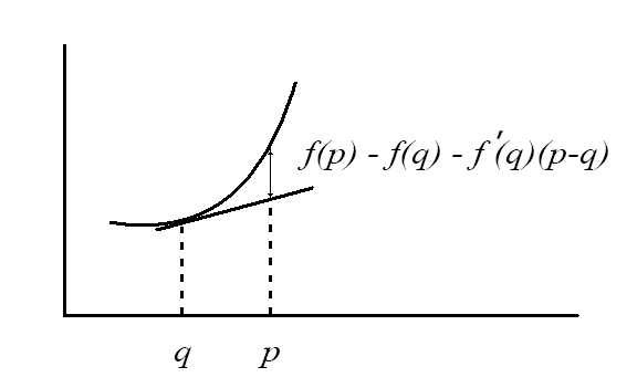
Figure 1: The Bregman distance $B_{f}(p\;\|\;q)$ is an indication of the increase in $f(p)$ over $f(q)$ above linear growth with slope $f^{\prime}(q)$.

The distances $B_{F}$ were introduced in by Bregman [4] along with an iterative algorithm for minimizing $B_{F}$ subject to linear constraints. Bregman distances have been used earlier by numerous authors to pose problems as generalized divergences. [7] used such divergences for generalized nonnegative matrix approximations. [1] used them for clustering applications. Other divergence minimization approaches have been tried for data mining and information retrieval. The concept of posing numerous problems of density estimation as KL divergence minimization problem has been long studied. It can be shown that KL divergence is a specialized case of Bregman divergence and hence the comprehensive success of such methods warrants a better investigation of Bregman divergence itself.

To develop the rest of this work we need a few definitions. Let $\Delta\subset\mathbb{R}^{r}$ and let $F:\Delta\rightarrow\mathbb{R}$ be a real valued function. We assume that $\Delta$ is a closed convex set, and that $F$ is strictly convex and $C^{1}$ on the interior of $\Delta$.

Definition 1 For $\mathbf{v}\in\mathbb{R}^{r}$ and $\mathbf{q}\in\Delta$ the Legendre Transform $\mathcal{L}_{F}(\mathbf{v},\mathbf{q})$ is defined as

$$\mathcal{L}_{F}(\mathbf{v},\mathbf{q})=\arg\displaystyle\min_{\mathbf{p}\in\Delta}B_{F}(\mathbf{p}\;\|\;\mathbf{q})+\mathbf{v}\cdot\mathbf{q}$$

Lemma 1 The mapping ${\mathbf{v},\mathbf{q}}\mapsto\mathcal{L}_{F}(\mathbf{v},\mathbf{q})$ defines a smooth action of $\mathbb{R}^{r}$ on $\Delta$ by

$$\mathcal{L}_{F}(\mathbf{v},\mathcal{L}_{F}(\mathbf{w},\mathbf{q}))=\mathcal{L}_{F}((\mathbf{v}+\mathbf{w}),\mathbf{q}).$$

The optimization problem which we consider is the following: let $A$ be an $n\times r$ matrix of linear constraints on $\mathbf{p}\in\Delta$. Let $\mathbf{q}_{0}\in\Delta$ be a default distribution, chosen such that $\nabla F(\mathbf{q}_{0})=0$. Finally, let $\tilde{\mathbf{p}}\in\Delta$ be given, which is considered the empirical distribution, since it typically arises from a set of training samples that determine the linear constraints.

We now define $\mathcal{P}(A,\tilde{\mathbf{p}})$ and $\mathcal{Q}(A,\mathbf{q}_{0})$ as

$$\mathcal{P}(A,\tilde{\mathbf{p}}) = \{\mathbf{p}\in\Delta|A\mathbf{p}=A\tilde{\mathbf{p}}\}$$

$$\mathcal{Q}(A,\mathbf{q}_{0}) = \{\mathbf{q}\in\Delta|\mathbf{q}=\mathcal{L}_{F}((\boldsymbol{\lambda}^{T}A),\mathbf{q}_{0}),\boldsymbol{\lambda}\in\mathbb{R}^{n}\}$$

The following well-known theorem [12] establishes the duality between the two natural projections of $B_{F}(\mathbf{p}\;\|\;\mathbf{q})$ with respect to the families $\mathcal{P}(A,\tilde{\mathbf{p}})$ and $\mathcal{Q}(A,\mathbf{q}_{0})$

Theorem 1 Suppose $B_{F}(\tilde{\mathbf{p}}\;\|\;\mathbf{q})<\infty$ and let $\bar{\mathcal{Q}}(A,\mathbf{q}_{0})=\mathrm{cl}(\mathcal{Q}(A,\mathbf{q}_{0}))$. Then there exists a unique $\mathbf{q}_{\star}\in\Delta$ such that

1. $\mathbf{q}_{\star}\in\mathcal{P}(A,\tilde{\mathbf{p}})\cap\mathcal{Q}(A,\mathbf{q}_{0})$

2. $B_{F}(\mathbf{p}\;\|\;\mathbf{q})=B_{F}(\mathbf{p}\;\|\;\mathbf{q}_{\star})+B_{F}(\mathbf{q}_{\star}\;\|\;\mathbf{q})$ for any $\mathbf{p}\in\mathcal{P}(A,\tilde{\mathbf{p}})$ and $\mathbf{q}\in\bar{\mathcal{Q}}(A,\mathbf{q}_{0})$

3. $\mathbf{q}_{\star}=\arg\displaystyle\min_{\mathbf{q}\in\bar{\mathcal{Q}}}B_{F}(\tilde{\mathbf{p}}\;\|\;\mathbf{q})$

4. $\mathbf{q}_{\star}=\arg\displaystyle\min_{\mathbf{p}\in\bar{\mathcal{P}}}B_{F}({\mathbf{p}}\;\|\;\mathbf{q}_{0})$

Moreover, any of these four properties determines $\mathbf{q}_{\star}$ uniquely.

Note that since we have defined $\nabla F(\mathbf{q}_{0})=0$, $\arg\displaystyle\min_{\mathbf{p}\in\bar{\mathcal{P}}}B_{F}({\mathbf{p}}\;\|\;\mathbf{q}_{0})=\arg\displaystyle\min_{\mathbf{p}\in\bar{\mathcal{P}}}F(\mathbf{p})$. Property $2$. is called the Pythagorean property since it resembles the Pythagorean theorem if we imagine that $B_{F}(\mathbf{p}\;\|\;\mathbf{q})$ is the square of Euclidean distance and $(\mathbf{p},\mathbf{q}_{\star},\mathbf{q})$ are the vertices of a right triangle.

4 Bregman Distance to Logistic Regression

In this section we study the minimization problem as mentioned in the previous section. By unconstrained we mean that the parameters $\lambda\in\mathbb{R}^{n}$ are free. We pose the logistic regression problem in the Bergman distance framework which was developed by Collins and Schapire [5].

The key idea is to write the function $F(\mathbf{p})$ as

$$F(\mathbf{p})=\sum_{i=1}^{m}p_{i}\ln p_{i}+(1-p_{i})\ln(1-p_{i})$$ (6)

The resulting Bergman distance is

$$D_{B}(\mathbf{p}\;\|\;\mathbf{q})=\sum_{i=1}^{m}p_{i}\ln\frac{p_{i}}{q_{i}}+(1-p_{i})\ln\frac{1-p_{i}}{1-q_{i}}$$ (7)

For this choice of $F$ the Legendre transform is found to be

$$\mathcal{L}_{F}(v,q)_{i}=\frac{q_{i}e^{-v_{i}}}{1-q_{i}+q_{i}e^{-v_{i}}}$$ (8)

Now we define the constraint matrix $A$ as $A_{ji}=y_{i}h_{j}(x_{i})$ from which we get $v_{i}=(\boldsymbol{\lambda}^{T}A)i=\sum_{j=1}^{n}\lambda_{j}y_{i}h_{j}(x_{i})$

Now, if we put $\mathbf{q_{0}}=(1/2)\mathbf{1}$ into eqn. 8 we get the logistic probability eqn. 2.

Also note that

$$D_{B}(\mathbf{0}\;\|\;\mathbf{q})=-\sum_{i=1}^{m}\ln(1-q_{i})$$ (9)

which gives

$$\ell(\mathbf{x},\mathbf{y}) = \sum_{i=1}^{m}\ln(1+e^{(-y_{i}f_{\boldsymbol{\lambda}}(x_{i})})$$

$$= D_{B}(\mathbf{0}\|\mathcal{L}_{F}(\boldsymbol{\lambda}^{T}A,\mathbf{q_{0}}))$$

where $f_{\boldsymbol{\lambda}}(x_{i})=\sum_{j=1}^{n}\lambda_{j}h_{j}(x_{i})$

Finally, we can write the equivalent optimization problem as

$$\displaystyle\min_{\mathbf{q}\in\bar{\mathcal{Q}}} D_{B}(\mathbf{0}\;\|\;\mathbf{q})$$

$$st A\mathbf{q}=0$$ (11)

where as before $\bar{\mathcal{Q}}=\mathrm{cl}(\mathcal{Q})$, where

$$Q=\left\{\begin{array}[]{c}\mathbf{q}\in\Delta:q_{i}=\sigma\left(\begin{array}[]{c}\sum_{j=1}^{n}\lambda_{j}y_{i}h_{j}(x_{i})\\ \end{array}\right),\boldsymbol{\lambda}\in\mathbb{R}^{n}\\ \end{array}\right\}$$

where $\sigma(x)=(1+e^{x})^{-1}$ is the Sigmoid function. For our choice of $\boldsymbol{q_{0}}=(1/2)\boldsymbol{1}$ we have $\mathcal{L}_{F}(\boldsymbol{v},\mathbf{q_{0}})_{i}=\sigma(v_{i})$ as shown in Eqn. 8. Also, since each of the elements of $\boldsymbol{q}$ is Sigmoid function output, therefore, $\Delta\in[0,1]^{m}$.

The key points to note in this derivation are

1. $\tilde{{\mathbf{p}}}\equiv 0$

2. $\boldsymbol{\lambda}\in\mathbb{R}^{n}$

The implication of the point (a.) above is that the constraints are homogenous. This is a strong assumption on the constraints. It so turns out that we can relax this constraint only when we put some additional constraints on the free parameter $\boldsymbol{\lambda}$. This points to a regularized scheme, where the first constraint is relaxed on the cost of putting some additional constraints on the second condition. We redefine the set $\mathcal{Q}$ as

$$Q=\{\mathbf{q}:q_{i}=\sigma(\sum_{j=1}^{n}\lambda_{j}y_{i}h_{j}(x_{i})),\boldsymbol{\lambda}\in\mathbb{R}^{n},\|\boldsymbol{\lambda}\|_{1}\leq c\}$$

We consider supervised learning in settings where there are many input features, but where there is a small subset of the features that is sufficient to approximate the target concept well. In supervised learning settings with many input features, over-fitting is usually a potential problem unless there is ample training data. For example, it is well known that for un-regularized discriminative models fit via training error minimization, sample complexity (i.e., the number of training examples needed to learn “well”) grows linearly with the VC dimension [14]. Further, the VC dimension for most models grows about linearly in the number of parameters [13], which typically grows at least linearly in the number of input features. Thus, unless the training set size is large relative to the dimension of the input, some special mechanism, such as regularization, which encourages the fitted parameters to be small is usually needed to prevent over-fitting.

Once we have defined our optimization problem our aim is to find a sequence of $q_{k}=\mathcal{L}_{F}(\boldsymbol{\lambda}_{k}^{T}A,\mathbf{q_{0}})$ which minimizes our cost function, all the while remaining feasible to the additional regularization constraint $\;\|\;\boldsymbol{\lambda}\;\|\;_{1}\leq c$.

5 Auxiliary Function

The idea of auxiliary functions was proposed by Della Pietra et al. [12]. The idea is analogous to EM algorithm and tries to bound the error for two iterations. Since we are dealing with distances which are defined to be positive, so the quantity $\|d_{t+1}-d_{t}\|=-(d_{t+1}-d_{t})$ for strict descent, which can be minimized iteratively, till convergence is achieved.

Definition 2   For a linear constraint matrix $A$, if $\boldsymbol{\lambda}\in\mathbb{R}^{n}$. A function $\mathcal{A}:\mathbb{R}^{n}\times\Delta\rightarrow\mathbb{R}$ is an auxiliary function for $L(q)=-B_{F}(\tilde{p}\;\|\;q)$ if

1. For all $q\in\Delta$ and $\boldsymbol{\lambda}\in\mathbb{R}^{n}$

   $L(\mathcal{L}_{F}(\boldsymbol{\lambda}^{T}A,\;q))\geq L(q)+\mathcal{A}(\boldsymbol{\lambda},q)$

2. $\mathcal{A}(\boldsymbol{\lambda},q)$ is continuous in $q\in\Delta$ and $C^{1}$ in $\boldsymbol{\lambda}\in\mathbb{R}^{n}$ with $\mathcal{A}(0,q)=0$ and

   $$\frac{d}{dt}|_{t=0}\mathcal{A}(t\boldsymbol{\lambda},q)=\frac{d}{dt}|_{t=0}L(\mathcal{L}_{F}(((t\boldsymbol{\lambda})^{T}A),q))$$

3. If $\boldsymbol{\lambda}=0$ is a minima of $\mathcal{A}(\boldsymbol{\lambda},q)$, then $q^{T}A=p_{0}^{T}A$.

Theorem 2    Suppose $q^{k}$ is any sequence in $\Delta$ with $q^{0}=q_{0}$ and $q^{k+1}=\mathcal{L}_{F}(\boldsymbol{\lambda}^{T}A,q)$ where $\boldsymbol{\lambda}\in\mathbb{R}^{n}$ satisfies

$$\mathcal{A}(\boldsymbol{\lambda}_{k},q^{k}) = \displaystyle\sup_{\boldsymbol{\lambda}}\mathcal{A}(\boldsymbol{\lambda},q^{k})$$

Then $L(q^{k})$ increases monotonically to $\displaystyle\max_{q\in\bar{\mathcal{Q}}}L(q)$ and $q^{k}$ converges to the distribution $q_{\star}=\arg\displaystyle\max_{q\in\bar{\mathcal{Q}}}L(q)$.

The proof of this theorem is elucidated in Della Pietra et al. [12]. We will mention the three lemmas on which the proof is based. Once the lemmas have been proved the proof for the theorem can be drawn simply from them. The three lemmas are

1. If $m\in\Delta$ is a cluster point of $\boldsymbol{q}^{(k)}$, then $\mathcal{A}(\boldsymbol{\lambda},\boldsymbol{q}^{(k)})\leq 0$ for all $\boldsymbol{\lambda}\in\mathbb{R}^{n}$.

2. If $m\in\Delta$ is a cluster point of $\boldsymbol{q}^{(k)}$, then $\frac{d}{dt}|_{t=0}L(\mathcal{L}_{F}(t\boldsymbol{\lambda}^{T}A,\boldsymbol{q}^{(k)}))=0$ for all $\boldsymbol{\lambda}\in\mathbb{R}^{n}$.

3. Suppose $\{\boldsymbol{q}^{(k)}\}$ is any sequence with only one cluster point $\boldsymbol{q}_{\star}$ . Then $\boldsymbol{q}^{(k)}$ converges to $\boldsymbol{q}_{\star}$.

6 Constrained Bregman Distance Minimization

Once we have shown the analogy between logistic regression and Bregman distances, we can proceed to find a suitable auxiliary function for our problem. One key observation is that we can write $q_{k+1}$ as a simple function of $q_{k}$ as follows

$$\boldsymbol{q}_{k+1} = \mathcal{L}_{F}((\boldsymbol{\lambda}_{k}+\boldsymbol{\delta}_{k})^{T}A,\;\boldsymbol{q_{0}})$$

$$= \mathcal{L}_{F}(\boldsymbol{\delta}_{k}^{T}A,\;\mathcal{L}_{F}(\boldsymbol{\lambda}_{k},\;\boldsymbol{q_{0}}))$$

$$= \mathcal{L}_{F}(\boldsymbol{\delta}_{k}^{T}A,\;\boldsymbol{q}_{k})$$

Let us denote $\mathbf{v}=\boldsymbol{\delta}_{k}^{T}A$, hence we can write $\boldsymbol{q}^{k+1}=\mathcal{L}_{F}(v,\boldsymbol{q}_{k})$. Now, from Eqn. 9, we can write

$$D_{B}(0\|\boldsymbol{q}^{k+1})-D_{B}(0\|\boldsymbol{q}^{k}) = \sum_{i=1}^{m}\ln(1-q_{i}+q_{i}e^{-v_{i}})$$

$$\leq \sum_{i=1}^{m}q_{i}(e^{-v_{i}}-1)$$

Substituting, $(\boldsymbol{\delta}^{T}A)_{i}=\mathbf{v}_{i}$, we define our auxiliary function as

$$\mathcal{A}(\boldsymbol{\delta},\boldsymbol{q})=\sum_{i=0}^{m}q_{i}(e^{-(\boldsymbol{\delta}^{T}A)_{i}}-1)$$ (12)

It can be easily verified that the above choice of auxiliary function satisfies the conditions mentioned in Def 2. Now we need to find a sequence of $\{\delta^{k}\}\rightarrow 0$ for which $\mathcal{A}(\boldsymbol{\delta},\boldsymbol{q})\leq 0$ and $\mathcal{A}(\boldsymbol{\delta},\boldsymbol{q})\rightarrow 0$ monotonically.

7 Algorithm

Assumptions: $F:\Delta\rightarrow\mathbb{R}$, such that $\{q\in\Delta:B_{F}(0\;\|\;\boldsymbol{q})\leq c\}$ where $c<\infty$.

Parameters: $\Delta\in[0,1]^{m}$, $F$ satisfying assumptions in part 1, and $\boldsymbol{q}_{0}=(1/2)\mathbf{1}$.

Input: Constraint matrix $A\in[-1,1]^{n\times m}$, where $A_{ji}=y_{i}h_{j}(x_{i})$, and $\sum_{j=1}^{n}|A_{ji}|\leq 1$.

Output: Denote $\mathcal{L}_{F}(\boldsymbol{\lambda}_{t}^{T}A,\boldsymbol{q}_{0})$ as $\mathcal{L}_{F}^{\boldsymbol{\lambda}_{t}}$. Generate a sequence of $\boldsymbol{\lambda_{1}},\boldsymbol{\lambda_{2}}\dots$ such that

$$\lim_{t\rightarrow\infty}B_{F}(0\|\mathcal{L}_{F}^{\boldsymbol{\lambda}_{t}})\rightarrow\arg\displaystyle\min_{\boldsymbol{\lambda}\in\mathbb{R}^{n}}B_{F}(0\|\mathcal{L}_{F}^{\boldsymbol{\lambda}})$$

subject to

$$\|\boldsymbol{\lambda}\|_{1}\leq\boldsymbol{u}$$

Let $\boldsymbol{\lambda}_{1}=\mathbf{0}$

For $k=1,2,\dots$

$~{}~{}\boldsymbol{q}^{k}=\mathcal{L}_{F}^{\boldsymbol{\lambda}_{k}}$

$~{}~{}\boldsymbol{\delta}_{k}=\arg\displaystyle\min_{\boldsymbol{\delta}\in\mathbb{R}^{n}}\sum_{i=1}^{m}q_{i}^{k}(e^{-(\boldsymbol{\lambda}^{T}A)_{i}}-1)$

$~{}~{}~{}~{}st:\;\|\;\boldsymbol{\lambda}_{k}+\boldsymbol{\delta}_{k}\;\|\;_{1}\leq\boldsymbol{u}$

Update $~{}~{}\boldsymbol{\lambda}_{k+1}=\boldsymbol{\lambda}_{k}+\boldsymbol{\delta}_{k}$

End For

8 A Primal-Dual method for $L1$ regularized Logistic Regression

The basic algorithm for the unconstrained case was proposed by [5], but their method finds a lower bound using the first order characteristics of the unconstrained minimizer. In our case we want to find the constrained minimizer of the auxiliary function. Since we need strict non-negative $\mathcal{A}(\boldsymbol{\delta},\boldsymbol{q})\leq 0$, so the new set of conditions are

$$\arg\displaystyle\min_{\boldsymbol{\delta}\in\mathbb{R}^{n}} \sum_{i=1}^{m}q_{i}(e^{-(\boldsymbol{\delta}^{T}A)_{i}}-1)$$ (13)

$$st: \;\|\;\boldsymbol{\lambda}+\boldsymbol{\delta}\;\|\;_{1}\leq u$$

$$\mathcal{A}(\boldsymbol{\delta},\boldsymbol{q})\leq 0$$

Analyzing the cost function more closely we find that it can be written as

$$e^{-(\boldsymbol{\delta}^{T}A)_{i}}-1 = e^{-\sum_{j=1}^{n}(\boldsymbol{\delta}_{j}A_{ji})_{i}}-1$$

$$= e^{-\sum_{j=1}^{n}(\boldsymbol{\delta}_{j}s_{ji}|A_{ji}|)}-1\hskip 28.45274pt$$

$$\leq \sum_{j=1}^{n}|A_{ji}|(e^{-(\boldsymbol{\delta}_{j}s_{ji})}-1)$$

where $s_{ji}=sign(A_{ji})$. Absorbing, this constraint into the cost function we get

$$\arg\displaystyle\min_{\boldsymbol{\delta}\in\mathbb{R}^{n}} \sum_{i=1}^{m}q_{i}\sum_{j=1}^{n}|A_{ji}|(e^{-(\boldsymbol{\delta}_{j}s_{ji})}-1)$$ (14)

$$st: \;\|\;\boldsymbol{\lambda}+\boldsymbol{\delta}\;\|\;_{1}\leq\boldsymbol{u}$$

$$\mathcal{A}(\boldsymbol{\delta},\boldsymbol{q})\leq 0$$

Now we define the two quantities

$$W_{j}^{+}(\boldsymbol{q}) = \displaystyle\sum_{sign(A_{ji})=+1}q_{i}|A_{ji}|$$

$$W_{j}^{-}(\boldsymbol{q}) = \displaystyle\sum_{sign(A_{ji})=-1}q_{i}|A_{ji}|$$

such that at iteration $k$ we have $W_{j}^{+}(\boldsymbol{q}_{t})$ and $W_{j}^{-}(\boldsymbol{q}_{t})$, then we can re-write the optimization problem as

$$\arg\displaystyle\min_{\boldsymbol{\delta}\in\mathbb{R}^{n}}\sum_{j=1}^{n}W_{j}^{+}(\boldsymbol{q}_{t})(e^{-\boldsymbol{\delta}_{j}}-1)+W_{j}^{-}(\boldsymbol{q}_{t})(e^{\boldsymbol{\delta}_{j}}-1)$$

$$st: \|\boldsymbol{\lambda}+\boldsymbol{\delta}\|_{1}\leq\boldsymbol{u}$$

$$\mathcal{A}(\boldsymbol{\delta},\boldsymbol{q})\leq 0$$

Adopting from [6], we can now introduce slack variables and write the penalty function as

$$\arg\displaystyle\min_{\boldsymbol{\delta},\boldsymbol{r},\boldsymbol{s},\boldsymbol{t},\boldsymbol{u}\in\mathbb{R}^{n}} \sum_{j=1}^{n}\mathcal{G}(\delta_{j})+a\mathbf{e}^{T}(s_{j}+t_{j})$$

$$st: \lambda_{j}+\delta_{j}+s_{j}-t_{j}=u_{j}$$

$$\mathcal{G}(\delta_{j})+r_{j}=0$$

$$s_{j},t_{j},r_{j}\geq 0$$

where $\mathcal{G}(\delta_{j})=W_{j}^{+}(\boldsymbol{q}_{t})(e^{-\boldsymbol{\delta}_{j}}-1)+W_{j}^{-}(\boldsymbol{q}_{t})(e^{\boldsymbol{\delta}_{j}}-1)$ and $j=\{1,\dots,n\}$.

Finally, introducing the log barrier function and absorbing the two terms $\lambda_{j}$ and $u_{j}$ into one term $c_{j}=u_{j}-\lambda_{j}$ we get

$$\arg\displaystyle\min_{\boldsymbol{\delta},\boldsymbol{r},\boldsymbol{s},\boldsymbol{t},\boldsymbol{c}\in\mathbb{R}^{n}}\sum_{j=1}^{n}\mathcal{G}(\delta_{j})+a\mathbf{e}^{T}(s_{j}+t_{j})-\mu\boldsymbol{\phi}(s_{j},t_{j},r_{j})$$

$$st: \delta_{j}+s_{j}-t_{j}=c_{j}$$

$$\mathcal{G}(\delta_{j})+r_{j}=0$$

where $\boldsymbol{\phi}(s_{j},t_{j},r_{j})=\log{s_{j}}+\log{t_{j}}+\log{r_{j}}$ and $\mu$ is the barrier parameter. As proposed in [6], we decompose the problem into a master problem and a sequence of sub-problems. We solve the following master problem for a sequence of barrier parameters $\{\mu_{k}\}$ such that $\displaystyle\lim_{k\rightarrow\infty}\mu_{k}=0+$ where the $+$ sign denotes converging to $0$ from the positive side

$$\min_{c}\sum_{j=1}^{N}F_{j}^{\star}(\mu,c)$$

The sequence of subproblems are exactly same as Eqn. 8, except the fact that the value of $c$ is held constant while solving the sub-problems. The $j^{th}$ sub-problem can now be written as

$$\arg\displaystyle\min_{{\delta},{r},{s},{t}\in\mathbb{R}} \mathcal{G}(\delta)+a(s+t)-\mu\boldsymbol{\phi}(s,t,r)$$ (18)

$$st: \delta+s-t=c$$

$$\mathcal{G}(\delta)+r=0$$

Proceeding as shown in Convex Optimization [3], Eqn. $11.53$, the modified KKT conditions can be expressed as $\mathfrak{r}_{t}(x,\lambda,\nu)=0$, (where the $(\lambda,\nu)$ are the multipliers, redefined again for consistency of notation), where we define

$$\mathfrak{r}_{t}(x,\lambda,\nu)=\left[\begin{array}[]{c}\nabla f_{0}(x)+J(x)^{T}\lambda+A^{T}\nu\\ (\lambda)f(x)-\mu\\ Ax-b\\ \end{array}\right]=0$$ (19)

where

$$x = \left[\begin{array}[]{c}\delta,~{}r,~{}s,~{}t\\ \end{array}\right]^{T}$$

$$f_{0}(x) = \mathcal{G}(\delta)+a(s+t)-\mu\boldsymbol{\phi}(s,t,r)$$

$$f(x) = \mathcal{G}(\delta)+r$$

$$J(x) = \left[\begin{array}[]{c}\Delta\mathcal{G}(\delta),\;1,\;0,\;0\\ \end{array}\right]^{T}$$

$$A = \left[\begin{array}[]{c}1,\;0,\;1,\;-1\\ \end{array}\right]^{T}$$

$$b = c$$

The Newton step can be now be formulated as

$$\left[\begin{array}[]{ccc}{\nabla^{2}f_{0}(x)+\lambda\nabla^{2}f(x)}&{J(x)^{T}}&{A^{T}}\\ {\lambda J(x)}&{f(x)}&{0}\\ {A}&0&0\\ \end{array}\right]\cdot$$ (26)

$$\left[\begin{array}[]{c}\nabla x\\ \nabla\lambda\\ \nabla\nu\\ \end{array}\right]=-\left[\begin{array}[]{c}\mathfrak{r}_{dual}\\ \mathfrak{r}_{cent}\\ \mathfrak{r}_{pri}\\ \end{array}\right]$$ (33)

where

$$\left[\begin{array}[]{c}\mathfrak{r}_{dual}\\ \mathfrak{r}_{cent}\\ \mathfrak{r}_{pri}\\ \end{array}\right]=\mathfrak{r}_{t}(x,\lambda,\nu)$$

9 Experiments and Results

In this section we report results for the experiments conducted for the new model proposed in this paper. The sparsity introduced by the $L1$ regularization is captured by conducting tests on randomly generated data. The loss-minimization curves remain similar to the unconstrained case since the unit slave problems mentioned in Eqn. 8 are convex. But the sparsity of feature vectors enables the dropping of redundant features and hence speeds up the iterations.

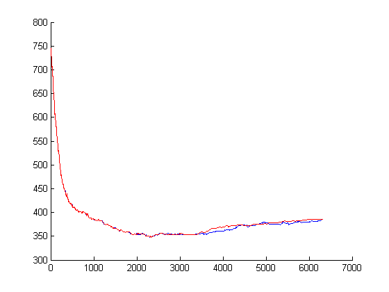
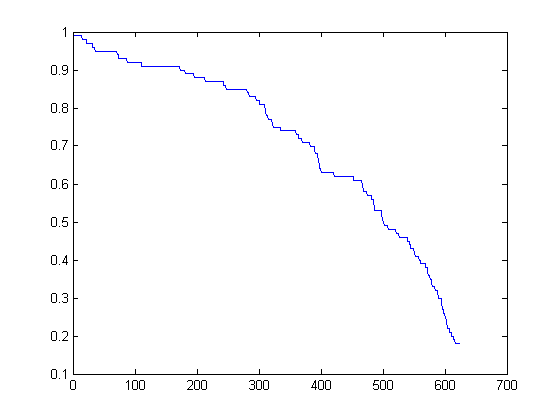
Figure 2: Left: Test Error, regularized (blue) and unconstrained (red) for $500$D, Right: Dropped features as a percentage of the total features.

In our experiments, we generated random data and classified it using a very noisy hyperplane. We investigate only $2$-class classification problems in this work. We investigate medium to high dimensional problems where the dimensionality ranges from $20-500$. We tested both the scenarios a) when the number of training points is of the order of the feature dimension and b) when the number of the training data points is an more than an order from the feature dimension. For every case the random data is first classified based on a random hyperplane and then we add Gaussian noise to the data dimensions based on a coin flip. The noise is assumed to be $\epsilon\sim\mathcal{N}(\mathbf{0},\sigma\mathbf{I})$, where $\sigma<1$. The key point of interest is the fact that since the procedure mentioned in this work decouples the features, and hence the features are dropped from the optimization scheme when the change $\nabla\delta_{i}$ drops below some threshold. One such comparative plots are shown in Fig. 2 (left). The sparsity of feature is shown in Fig. 2 (right).

For comparing with other algorithms we run the logistic classifier over public domain data namely the Wisconsin Diagnostic Breast Cancer (WDBC) data set and the Musk data base (Clean $1$ and $2$) [10]. The WDBC data has $569$ instances with $30$ real valued features. There are 357 benign (positive) instances and $212$ malignant (negative) instances. The best reported result is $97.5\%$ using decision trees constructed by linear programming [9, 2]. Our method generate $16$ fakse negatives and $23$ false positives, totaling $39$ errors with an accuracy of $93.15\%$. The training and testing errors are shown in Fig. 3 (left).

The musk clean $1$ data-set describes a set of 92 molecules of which 47 are judged by human experts to be musks and the remaining 45 molecules are judged to be non-musks. Similarly, the musk clean $2$ data base describes a set of $102$ molecules of which $39$ are musks and the remaining $63$ molecules are non-musks. The $166$ features that describe these molecules depend upon the exact shape, or conformation, of the molecule. Multiple confirmations for each instance were created, which after pruning amount to $476$ conformations for clean $1$ and $6598$ for clean $2$ data-set. The many-to-one relationship between feature vectors and molecules is called the ”multiple instance problem”. When learning a classifier for this data, the classifier should classify a molecule as ”musk” if ANY of its conformations is classified as a musk. A molecule should be classified as ”non-musk” if NONE of its conformations is classified as a musk.

We report results for tests conducted on the two data-bases. The training and test plots for the clean $2$ data are shown in Fig. 3 (right). We compare our method L$1$ Logistic Regression based on Bregman Distances (L1LRB) against published results and our method outperforms most of them. The comparative results are shown in Table. 1 and Table. 2. Also note that the poor performance of C$4.5$ algorithm has been attributed to the fact that it does not take the multi-instance nature of the problem into consideration for training. We did not take this consideration while training and still our method ranks as the top $2$ for among all the reported results. The details for the other methods mentioned have been discussed in [8].

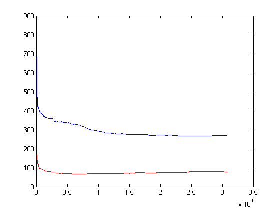
Figure 3: Train Error (blue) and Test Error (red). Left: WDBC data, Right: Musk Clean $2$ data.

Algorithm	TP	FN	FP	TN	% Acc
L1LRB	$45$	$2$	$2$	$43$	$95.6$
Iter-discrim APR	$42$	$5$	$2$	$43$	$92.4$
GFS-Elim-kde APR	$46$	$1$	$7$	$38$	$91.3$
All-pos APR	$36$	$11$	$7$	$38$	$80.4$
Back-prop	$45$	$2$	$21$	$24$	$75.0$
C4.5(pruned)	$45$	$2$	$24$	$21$	$68.5$

Table 1: Comparative results for the Musk Clean $1$ database.

Algorithm	TP	FN	FP	TN	% Acc
Iter-discrim APR	$30$	$9$	$2$	$61$	$89.2$
L1LRB	$30$	$9$	$6$	$57$	$85.29$
GFS-Elim-kde APR	$32$	$7$	$13$	$50$	$80.4$
GFS-El-count APR	$31$	$8$	$17$	$46$	$75.5$
All-pos APR	$34$	$5$	$23$	$40$	$72.6$
Back-prop	$16$	$23$	$10$	$53$	$67.7$
GFS-All-Pos APR	$37$	$2$	$32$	$31$	$66.7$
Most Freq Class	$0$	$39$	$0$	$63$	$61.8$
C4.5(pruned)	$32$	$7$	$35$	$28$	$58.8$

Table 2: Comparative results for the Musk Clean $2$ database.

10 Conclusion and extensions

We posed the problem of $L1$ regularized logistic regression as a constrained Bregman distance minimization problem and posed the optimization problem as a decoupled primal-dual problem in each of the dimensions of the parameter vector. The optimization technique mentioned in this work takes help from the strict feasibility properties of primal dual methods and hence guarantee the convergence of the algorithm. Comparative results on published data-sets have prove the strength of the regularized method.

References

[1]
A. Banerjee, S. Merugu, I. Dhillon, and J. Ghosh.
Clustering with bregman divergences.
In SIAM International Conference on Data Mining (SDM), 2004.
[2]
K. P. Bennett.
Decision tree construction via linear programming.
In Proceedings of the Midwest Artificial Intelligence
and Cognitive Science Society, pages 97–101, 1992.
[3]
S. Boyd and L. Vandenberghe.
Convex Optimization.
Cambridge University Press, 2004.
[4]
L. M. Bregman.
The relaxation method of finding the common point of convex sets and
its application to the solution of problems in convex programming.
In Computational Mathematics and Mathematical Physics,
volume 7, pages 200–217, U.S.S.R, 1967.
[5]
M. Collins, R. E. Schapire, and Y. Singer.
Logistic regression, adaboost and bregman distances.
Mach. Learn., 48(1-3):253–285, 2002.
[6]
A.-V. de Miguel.
Two Decomposition Algorithms for Nonconvex Optimization Problems
with Global Variables.
PhD thesis, Stanford University, April 2001.
[7]
I. Dhillon and S. Sra.
Generalized nonnegative matrix approximations with bregman
divergences.
In Y. Weiss, B. Schölkopf, and J. Platt, editors, Advances
in Neural Information Processing Systems 18, pages 283–290. MIT Press,
Cambridge, MA, 2006.
[8]
T. G. Dietterich, R. H. Lathrop, and T. Lozano-Perez.
Solving the multiple instance problem with axis-parallel rectangles.
Artificial Intelligence, 89(1-2):31–71, 1997.
[9]
O. L. Mangasarian, W. N. Street, and W. H. Wolberg.
Breast cancer diagnosis and prognosis via linear programming.
In Operations Research, volume 43, pages 570–577, July-August
1995.
[10]
D. J. Newman, S. Hettich, C. L. Blake, and C. J. Merz.
UCI repository of machine learning databases, 1998.
[11]
A. Ng.
Feature selection, vs. regularization, and rotational
invariance.
In In Proceedings of the twenty-first international conference
on Machine learning (ICML), pages 78–85, New York, NY, USA, 2004. ACM
Press.
[12]
S. D. Pietra, V. D. Pietra, and J. Lafferty.
Inducing features of random fields.
In IEEE Transactions on Pattern Analysis and Machine
Intelligence, volume 19, pages 380–393, 1997.
[13]
V. N. Vapnik.
Estimation of Dependences Based on Empirical Data.
Springer-Veriag, 1982.
[14]
V. N. Vapnik and A. Y. Chervonenkis.
Theory of Pattern Recognition.
Nauka, Moscow, 1974.