Nodes in the gap structure of the iron-arsenide superconductor Ba(Fe_1-xCo_x)₂As₂ from $c$-axis heat transport measurements

Abstract

The thermal conductivity $\kappa$ of the iron-arsenide superconductor Ba(Fe_1-xCo_x)₂As₂ was measured down to 50 mK for a heat current parallel ($\kappa_{c}$) and perpendicular ($\kappa_{a}$) to the tetragonal $c$ axis, for seven Co concentrations from underdoped to overdoped regions of the phase diagram ($0.038\leq x\leq 0.127$). A residual linear term $\kappa_{c0}/T$ is observed in the $T\to 0$ limit when the current is along the $c$ axis, revealing the presence of nodes in the gap. Because the nodes appear as $x$ moves away from the concentration of maximal $T_{c}$, they must be accidental, not imposed by symmetry, and are therefore compatible with an $s_{\pm}$ state, for example. The fact that the in-plane residual linear term $\kappa_{a0}/T$ is negligible at all $x$ implies that the nodes are located in regions of the Fermi surface that contribute strongly to $c$-axis conduction and very little to in-plane conduction. Application of a moderate magnetic field (e.g. $H_{\rm c2}/4$) excites quasiparticles that conduct heat along the $a$ axis just as well as the nodal quasiparticles conduct along the $c$ axis. This shows that the gap must be very small (but non-zero) in regions of the Fermi surface which contribute significantly to in-plane conduction. These findings can be understood in terms of a strong ${\bf k}$ dependence of the gap $\Delta({\bf k})$ which produces nodes on a Fermi surface sheet with pronounced $c$-axis dispersion and deep minima on the remaining, quasi-two-dimensional sheets.

I Introduction

The discovery of superconductivity in iron arsenides,Kamihara2008 with transition temperatures exceeding 50 K,Zhi-An2008 breaks the monopoly of cuprates as the only family of high-temperature superconductors, and revives the question of the pairing mechanism. Because the mechanism is intimately related to the symmetry of the order parameter, which is in turn related to the ${\bf k}$ dependence of the gap function $\Delta({\bf k})$, it is important to determine the gap structure in the iron-based superconductors, just as it was crucial to establish the $d$-wave symmetry of the gap in cuprate superconductors. The gap structure of iron-based superconductors has been the subject of numerous studies (for recent reviews, see Refs. Ishida2009, ; Mazin2010, ). Here, we focus on the material BaFe₂As₂, in which superconductivity can be induced either by applying pressure Alireza2009 or by various chemical substitutions, such as K for Ba (K-Ba122) Rotter2008 or Co for Fe (Co-Ba122).Sefat2008 In the case of Co-Ba122, single crystals have been grown with compositions that cover the entire superconducting phase (see Fig. 1).Ni2008 ; Nandi2010 ; Fernandes2010

Two sets of experiments on doped BaFe₂As₂ appear to give contradictory information. On the one hand, angle-resolved photoemission spectroscopy (ARPES) detects a nodeless, isotropic superconducting gap on all sheets of the Fermi surface in K-Ba122 Nakayama2009 and in optimally-doped Co-Ba122,Terashima2009 and tunneling studies in K-Ba122 detect two full superconducting gaps.Samuely2009 The magnitude of the gaps in ARPES is largest on Fermi surfaces where a density-wave gap develops in the parent compounds.Xu2009 This is taken as evidence for an s_± pairing state driven by antiferromagnetic correlations.Mazin2008 ; Kuroki2008 ; Vorontsov2008 ; Mazin2010 On the other hand, the penetration depth in Co-Ba122,Gordon2009a ; Gordon2009 the spin-lattice relaxation rate in K-Ba122,Fukazawa2009 and the in-plane thermal conductivity in K-Ba122 Luo2009 and Co-Ba122,Tanatar2010 ; Dong2010 for example, are inconsistent with a gap that is large everywhere on the Fermi surface. Note, however, that the evidence for deep minima in the gap is particularly clear in the overdoped regime,Fukazawa2009 ; Tanatar2010 ; Martin2010 a regime which has not so far been probed by either ARPES or tunneling.

Another possible explanation for the apparent discrepancy between the two sets of experimental results is a different sensitivity to the $c$-axis component ($k_{z}$) of the quasiparticle ${\bf k}$ vector, taking into account the three-dimensional (3D) character of the Fermi surface. Sefat2008 ; Malaeb2009 ; Utfeld2010 ; Kemper2009 ; Analytis2009 ; Tanatar2009 ; Tanatar2009a Nodes along the $c$ axis were suggested theoretically to explain the discrepancy between ARPES, penetration depth and NMR studies.Laad2009 ; Graser2010 A variation of the gap magnitude as a function of $k_{z}$ was suggested in experimental studies of the neutron resonances in optimally-doped Ni-Ba122.Chi2009 It was also invoked to explain the temperature dependence of the penetration depth in Co-Ba122 Gordon2009 and its $a-c$ anisotropy in Ni-Ba122.Martin2010 Clearly, it has become important to resolve the 3D structure of the superconducting gap function in doped BaFe₂As₂.

Heat transport measured at very low temperatures is one of the few directional bulk probes of the gap structure. The existence of a finite residual linear term $\kappa_{0}/T$ in the thermal conductivity $\kappa(T)$ as $T\to 0$ is unambiguous evidence for the presence of nodes in the gap,Hirschfeld1988 ; Graf1996 ; Durst2000 ; Taillefer1997 ; Suzuki2002 and thus by measuring $\kappa(T)$ as a function of direction in the crystal, one can locate the position of nodes on the Fermi surface.Hirschfeld1988 ; Graf1996 ; Shakeripour2009a ; Shakeripour2007 Here, we report measurements of heat transport in Ba(Fe_1-xCo_x)₂As₂ for a current direction both parallel and perpendicular to the $c$ axis of the tetragonal (or orthorhombic) crystal structure. Our main finding is a sizable residual linear term $\kappa_{0}/T$ for a current along the $c$ axis, and a negligible one for a current perpendicular to it. This implies the presence of nodes in the gap in regions of the Fermi surface that dominate the $c$-axis conduction and contribute little to in-plane conduction. Our study shows that the gap structure of Co-Ba122 depends on the 3D character of the Fermi surface in a way that varies strongly with $x$.

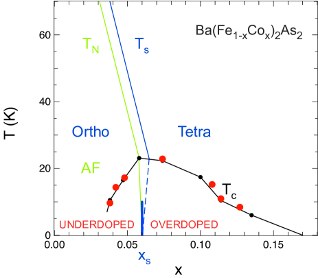
Figure 1: Phase diagram of Ba(Fe_1-xCo_x)₂As₂ as a function of Co concentration $x$, showing the orthorhombic phase below $T_{s}$ (blue), the antiferromagnetic (AF) phase below $T_{N}$ (green), and the superconducting phase below $T_{c}$ (small black dots), as determined from resistivity, magnetization and heat capacity data,Ni2008 and from x-ray Nandi2010 and neutron Fernandes2010 data. Red circles mark the $T_{c}$ value of seven samples measured in the present study (the $c$-axis samples labelled A in Table I), indicating the range of concentrations covered. The vertical dashed line at $x=0.06$ marks the approximate location of the critical concentration $x_{s}$ where at $T=0$ the system goes from orthorhombic (Ortho) in the underdoped region (to the left) to tetragonal (Tetra) in the overdoped region (to the right).Nandi2010 At $T=0$, the AF phase also ends close to $x=0.06$.Fernandes2010

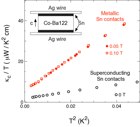
Figure 2: Temperature dependence of the thermal conductivity $\kappa$, plotted as $\kappa/T$ vs $T^{2}$, measured along the $c$ axis in a Co-Ba122 sample with $x=0.127$, using the two-probe technique, for three values of the applied field: $H=0.0$, 0.05 and 0.10 T. At $H=0$, the total thermal resistance of sample plus contacts is dominated by the very high thermal resistance of the two superconducting tin contacts. At $H=50$ mT, tin is no longer superconducting and the thermal resistance of the two contacts has become negligible compared to the sample resistance. In this case, extrapolation of $\kappa/T$ to $T$=0 gives us almost exactly the residual linear term in the sample’s thermal conductivity. Increasing $H$ slightly beyond 50 mT, for example to 100 mT, leads to no further change in the data. This shows that measurements in $H=50$ mT reveal the intrinsic zero-field behavior of the sample. The inset shows the arrangement of the tin (Sn) contacts and the silver (Ag) wires on the sample.

Table 1: Properties of the twelve $c$-axis samples of Co-Ba122 used in this study. $x$ is the Co concentration measured by wavelength dispersive microprobe analysis. The superconducting transition temperature $T_{c}$ is the temperature at which the resistivity goes to zero. The values of the upper critical field $H_{c2}$ needed to suppress superconductivity in Co-Ba122 at $T\to 0$ are taken from Refs. Ni2008, and Kano2009, . ($H_{c2}(T)$ is defined as the end, or ‘offset’, of the superconducting drop in $\rho(T)$ vs $H$). The residual resistivity $\rho_{c0}$ is obtained by a smooth extrapolation of the $\rho_{c}(T)$ data to $T=0$, as shown in Fig. 3. The normal-state residual linear term in the thermal conductivity, $\kappa_{\rm cN}/T$, is obtained from the Wiedemann-Franz law applied to $\rho_{c0}$ (see text). The zero-field residual linear term, $\kappa_{c0}/T$, is obtained by extrapolating to $T=0$ the zero-field thermal conductivity $\kappa_{c}$ with a linear fit to $\kappa_{c}/T$ vs $T^{2}$, as shown in Fig. 5. $\kappa_{c0}/T$ is also expressed as a fraction of the normal-state $\kappa_{\rm cN}/T$, denoted $\kappa_{0}/\kappa_{\rm N}\equiv(\kappa_{\rm 0}/T)/(\kappa_{\rm N}/T)$.

$x$	Sample	$T_{c}$	$H_{c2}$	$\rho_{c0}$	$\kappa_{\rm cN}/T$	$\kappa_{c0}/T$	$\kappa_{0}/\kappa_{\rm N}$
		(K)	(T)	$(\mu\Omega$ cm)	($\mu$W/K2 cm)
0.038	A	9.7	30	1935	12.7	6.1	0.48
0.042	A	14.4	40	1980	12.4	2.3	0.19
0.042	B	13.7	40	2115	11.6	2.9	0.25
0.048	A	17.2	45	2535	9.7	0.6	0.06
0.048	B	17.2	45	3045	8.0	0.8	0.10
0.074	A	22.9	60	1030	23.8	0.9	0.04
0.074	B	24.1	60	1140	21.5	0.2	0.01
0.108	A	15.2	30	1560	15.7	2.3	0.15
0.108	B	14.6	30	1770	13.8	1.6	0.12
0.114	A	11.0	20	1415	17.3	3.8	0.22
0.127	A	8.4	15	1500	16.3	5.6	0.34
0.127	B	9.3	15	1130	21.7	6.8	0.31

II Experimental

II.1 Samples

Single crystals of Ba(Fe_1-xCo_x)₂As₂ were grown from FeAs:CoAs flux, as described elsewhere.Ni2008 The doping level in the crystals was determined by wavelength dispersive electron probe microanalysis, which gave a Co concentration, $x$, roughly 0.7 times the flux load composition (or nominal content). We studied seven compositions: underdoped, with $x=0.038$, 0.042, and 0.048; overdoped, with $x=0.074$, 0.108, 0.114, and 0.127. In this Article, ‘underdoped’ and ‘overdoped’ refer to concentrations respectively below and above the critical concentration $x_{s}\simeq 0.06$ at which the system at $T=0$ goes from orthorhombic (below) to tetragonal (above).Nandi2010 The $T_{c}$ value for each composition is shown on the phase diagram in Fig. 1. A total of twelve $c$-axis and nine $a$-axis samples were studied; their characteristics are listed in Tables I and II, respectively. Three of the $a$-axis samples were the subject of a previous study (0.074-B, 0.108-A, and 0.114-B).Tanatar2010

II.2 Two-probe transport measurements

Thermal conductivity was measured in a standard one-heater-two-thermometer technique.Sutherland2003 The magnetic field $H$ was applied along the [001] or $c$-axis direction of the crystal structure, which is tetragonal for overdoped samples and orthorhombic for underdoped samples at low temperatures. Data were taken on warming after having cooled in a constant field applied above $T_{c}$ to ensure a homogeneous field distribution.

It is conventional to measure electrical and thermal resistance in a four-probe configuration to avoid the contribution of contact resistances. This is what was done for data taken with a current in the basal plane ($J~{}||~{}a$, in the notation appropriate for the tetragonal phase), as described elsewhere.Luo2009 ; Tanatar2010 For a current along the $c$ axis ($J~{}||~{}c$), however, the four-probe technique is difficult because of the strong tendency of iron-arsenide crystals to exfoliation, which makes it difficult to cut samples thick enough in the $c$ direction to attach four contacts.Tanatar2009 ; Tanatar2009a Consequently, $c$-axis transport was measured using a two-probe technique, which is valid provided contact resistances are much smaller than the sample resistance.

Contacts to the $c$-axis samples were made using silver wires (of 50 $\mu$m diameter), soldered to the top and bottom surfaces of the sample with ultrapure tin (see inset of Fig. 2). The contact making and properties are described in detail in Ref. Tanatar2010a, . In brief, these contacts are characterized by a surface area resistivity in the n$\Omega$ cm² range, which, for a typical sample size, yields a contact resistance below 10 $\mu\Omega$. This is negligible compared to a typical sample resistance in the normal state, of the order of 10 m$\Omega$.

Because tin is a superconductor, the thermal resistance of the contacts at very low temperature is large. We therefore have to apply a small magnetic field to suppress the superconductivity of tin and make it a normal metal, with the very low electrical and thermal resistance mentioned above. A field of 50 mT is sufficient to do this. In Fig. 2, we compare data obtained with $H=0.00$, 0.05 and 0.10 T. The effect of switching off the contact resistance with the field is clear, and once tin has gone normal, the data is independent of a further small increase in $H$. We therefore regard the data taken at $H=0.05$ T as representative of the zero-field state of the sample.

Table 2: Properties of the nine $a$-axis samples of Co-Ba122 used in this study. $x$, $T_{c}$, $H_{c2}$ and $\kappa_{0}/\kappa_{\rm N}$ are defined in Table I. The residual resistivity $\rho_{a0}$ is obtained by a smooth extrapolation of the $\rho_{a}(T)$ data to $T=0$, as shown in Fig. 4. The normal-state residual linear term in the thermal conductivity, $\kappa_{\rm aN}/T$, is obtained from the Wiedemann-Franz law applied to $\rho_{a0}$. The zero-field residual linear term, $\kappa_{a0}/T$, is obtained by extrapolating to $T=0$ the zero-field thermal conductivity $\kappa_{a}$ with a power-law fit to $\kappa_{a}/T$ (see text), as shown in Fig. 7. Note that the magnitude of $\kappa_{a0}/T$, whether positive or negative, is in all cases lower than the uncertainty in the extrapolation (see Fig. 9).

$x$	Sample	$T_{c}$	$H_{c2}$	$\rho_{a0}$	$\kappa_{\rm aN}/T$	$\kappa_{a0}/T$	$\kappa_{0}/\kappa_{\rm N}$
		(K)	(T)	$(\mu\Omega$ cm)	($\mu$W/K2 cm)
0.042	A	13.0	40	200	123	1	0.01
0.042	B	14.2	40	235	104	0	0
0.048	A	16.7	45	150	163	2	0.01
0.074	A	22.2	60	62	395	-1	0
0.074	B	22.2	60	82	299	3	0.01
0.108	A	14.8	30	59	415	-1	0
0.114	A	10.8	20	59	415	-9	-0.02
0.114	B	10.2	20	56	438	-13	-0.03
0.127	A	8.2	15	48	510	17	0.03

II.3 Electrical resistivity

In Fig. 3, we show the temperature dependence of the electrical resistivity $\rho_{c}(T)$ of our $c$-axis samples, measured in a two-probe configuration. In all samples, the resistivity follows qualitatively the temperature dependence reported previously.Tanatar2009 Data for the $a$-axis samples are shown in Fig. 4. A smooth extrapolation of $\rho(T)$ to $T=0$ yields the residual resistivity $\rho_{0}$ listed in Table I for $c$-axis samples and in Table II for $a$-axis samples. The uncertainty associated with the extrapolation of $\rho(T)$ to $T=0$ is approximately $\pm~{}5~{}\%$. Due to the uncertainty in measuring the geometric factor, the absolute value of the resistivity has an error bar of approximately $\pm$ 20 % for $a$-axis samples and a factor of 2 uncertainty for $c$-axis samples. Tanatar2009 ; Tanatar2009a ; Laad2009 The higher $\rho_{0}$ values in the underdoped regime are due to a reconstruction of the Fermi surface in the antiferromagnetic phase. The residual resistivity $\rho_{0}$ is used to determine the normal-state thermal conductivity $\kappa_{\rm N}/T$ in the $T=0$ limit via the Wiedemann-Franz law, $\kappa_{\rm N}/T=L_{0}/\rho_{0}$, where $L_{0}=2.45~{}\times$ 10^-8 W $\Omega$ / K². Because the same contacts are used for electrical and thermal measurements, the relative geometric-factor uncertainty between the measured $\kappa$ and this electrically-determined $\kappa_{\rm N}$ is minimal.

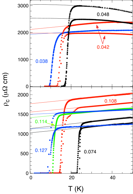
Figure 3: Temperature dependence of the $c$-axis resistivity $\rho_{c}(T)$ for the twelve $c$-axis crystals of Ba(Fe_1-xCo_x)₂As₂ studied here, with Co concentrations $x$ as indicated. Top and bottom panels show underdoped and overdoped samples, respectively. Circles and triangles of the same color correspond to two different crystals at the same doping, respectively labelled A and B (see Table I). The lines show how the data is extrapolated to $T=0$, to determine the value of the residual resistivity $\rho_{c0}$, given in Table I.

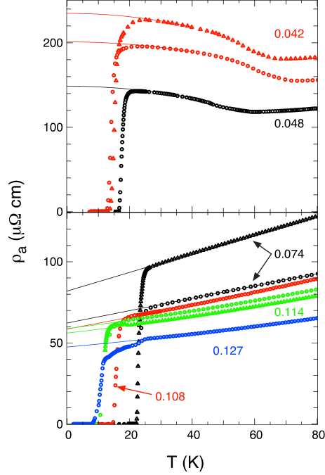
Figure 4: Temperature dependence of the $a$-axis (in-plane) resistivity $\rho_{a}(T)$ for the nine $a$-axis crystals of Ba(Fe_1-xCo_x)₂As₂ studied here, with Co concentrations $x$ as indicated. Top and bottom panels show underdoped and overdoped samples, respectively. Circles and triangles of the same color correspond to two different crystals at the same doping, respectively labelled A and B (see Table II). The lines show how the data is extrapolated to $T=0$, to determine the value of the residual resistivity $\rho_{a0}$, given in Table II.

III Results

III.1 Heat transport in the $c$ direction

The thermal conductivity of solids is the sum of electronic and phononic contributions: $\kappa=\kappa_{e}+\kappa_{p}$. In the $T=0$ limit, the electronic conductivity is linear in temperature: $\kappa_{e}\propto T$. In practice, the way to extract $\kappa_{e}$ is to extrapolate $\kappa/T$ to $T=0$, and thus obtain the purely electronic residual linear term, $\kappa_{0}/T$.Shakeripour2009a ; Sutherland2003 ; Hawthorn2007 If one can neglect electron-phonon scattering, as one usually can deep in the superconducting state, then the mean free path of phonons as $T\to 0$ is controlled by the sample boundaries. If those boundaries are rough, the scattering is diffuse and the mean free path is constant, such that the phonon conductivity $\kappa_{p}\propto T^{3}$. (Phonons can also be scattered by twin boundaries and grain boundaries.) If the sample boundaries are smooth, specular reflection yields a temperature-dependent mean free path, and $\kappa_{p}\propto T^{\alpha}$, typically with $2<\alpha<3$.Sutherland2003 ; Li2008

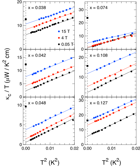
Figure 5: Temperature dependence of the $c$-axis thermal conductivity $\kappa_{c}$, plotted as $\kappa_{c}/T$ vs $T^{2}$, for six samples of Ba(Fe_1-xCo_x)₂As₂, with $x$ as indicated, in a magnetic field $H=0.05$, 4, and 15 T (data taken at other fields are not shown for clarity). These are six of the seven samples labelled A in Table I. The lines are a linear fit to the data below $T^{2}=0.015$ K², used to extract the residual linear term $\kappa_{c0}/T$ as the extrapolation of $\kappa_{c}/T$ to $T=0$. The values of $\kappa_{c0}/T$ are listed in Table I for $H=0$, and plotted vs $H$ in Fig. 6, for all twelve $c$-axis samples. Solid black squares on the $T=0$ axis (dashed line) give the residual linear term in the normal-state thermal conductivity, $\kappa_{\rm cN}/T$, obtained from the residual resistivity $\rho_{c0}$ of the sample via the Wiedemann-Franz law (see Table I).

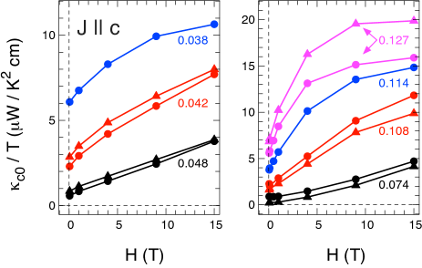
Figure 6: Field dependence of the residual linear term $\kappa_{c0}/T$ in the $c$-axis thermal conductivity of our twelve $c$-axis single crystals of Co-Ba122, with $x$ as indicated. Underdoped compositions are shown on the left, overdoped compositions on the right. For five concentrations, two different crystals with nominally the same $x$ value, labelled A (circles) and B (triangles), were measured (see Table I).

In Fig. 5, we show the thermal conductivity $\kappa_{c}$ of our $c$-axis samples, plotted as $\kappa_{c}/T$ vs $T^{2}$, for magnetic fields from $H=0.05$ to 15 T. Below $T\simeq 0.15$ K, the curves are linear, consistent with diffuse phonon scattering on the sample boundaries of our $c$-axis samples, which are indeed characterized by rough side surfaces. We obtain $\kappa_{e}/T\equiv\kappa_{0}/T$ by extrapolating $\kappa/T$ to $T=0$ using a linear fit below $T^{2}=0.015$ K². The error bar on this extrapolation is approximately $\pm~{}0.5~{}\mu$W/K² cm, for all $c$-axis samples. The value of $\kappa_{c0}/T$ thus obtained is plotted as a function of field $H$ in Fig. 6, for all twelve $c$-axis samples. For five concentrations, we have a pair of crystals with nominally the same Co concentration. As can be seen, the two curves in each pair are in good agreement with each other, well within the uncertainty in the geometric factor. The zero-field values are listed in Table I. They range from $\kappa_{c0}/T<1~{}\mu$W/K² cm at $x=0.048$ and 0.074 to $\kappa_{c0}/T\simeq 6~{}\mu$W/K² cm at $x=0.038$ and 0.127.

The normal-state residual linear term $\kappa_{\rm N}/T$ was estimated using the values of $\rho_{0}$ through application of the Wiedemann-Franz law. The value of $\kappa_{\rm N}/T$ is shown as a solid black square on the $y$ axis of Fig. 5. For the most heavily overdoped samples, with $x=0.127$, a magnetic field of 15 T is sufficient to reach the normal state, where $\kappa_{0}/T$ saturates to its normal-state value $\kappa_{\rm N}/T$. This allows us to check the Wiedemann-Franz law. For sample A, $\kappa_{c0}/T=16.0\pm 0.5~{}\mu$W/K² cm at $H=15$ T, while $\kappa_{\rm N}/T=16.3\pm 0.8~{}\mu$W/K² cm; for sample B, $\kappa_{c0}/T=20.0\pm 0.5~{}\mu$W/K² cm at $H=15$ T, while $\kappa_{\rm N}/T=21.7\pm 1.1~{}\mu$W/K² cm. Within error bars, associated with extrapolations to get $\kappa_{0}/T$ and $\rho_{0}$, the Wiedemann-Franz law is satisfied in both samples.

III.2 Heat transport in the $a$ direction

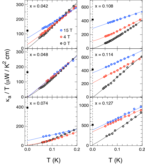
Figure 7: Temperature dependence of the $a$-axis thermal conductivity $\kappa_{a}$, plotted as $\kappa_{a}/T$ vs $T$, for six samples of Ba(Fe_1-xCo_x)₂As₂, with $x$ as indicated, in a magnetic field $H=0$, 4, and 15 T (data taken at other fields are not shown for clarity). These are the six samples labelled A in Table II. The lines are a power-law fit to the data below $T=0.3$ K, namely $\kappa/T=a+bT^{\alpha-1}$. The fit is used to extrapolate $\kappa_{a}/T$ to $T=0$ and thus obtain the residual linear term $\kappa_{a0}/T$. The power $\alpha$ is in the range from 2 to 2.5. The values of $\kappa_{a0}/T$ are listed in Table II for $H=0$, and plotted vs $H$ in Fig. 8, for all nine $a$-axis samples. Solid black squares on the $T=0$ axis give the residual linear term in the normal-state thermal conductivity, $\kappa_{\rm aN}/T$, obtained from the residual resistivity $\rho_{a0}$ of the sample via the Wiedemann-Franz law (see Table II).

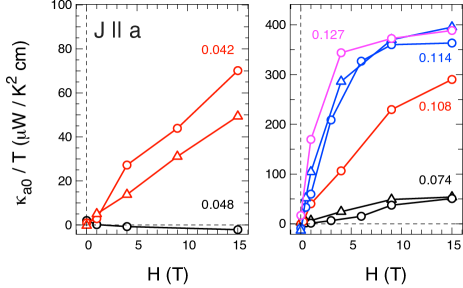
Figure 8: Field dependence of the residual linear term $\kappa_{a0}/T$ in the $a$-axis thermal conductivity of our nine $a$-axis single crystals of Co-Ba122, with $x$ as indicated. Underdoped compositions are shown of the left, overdoped compositions on the right. For three concentrations, two different crystals with nominally the same $x$ value, labelled A (circles) and B (triangles), were measured (see Table II).

In Fig. 7, we show the thermal conductivity $\kappa_{a}$ for six of our nine $a$-axis samples, plotted as $\kappa_{a}/T$ vs $T$, for magnetic fields from $H=0$ to 15 T. Unlike in the $c$-axis samples, the phonon conductivity $\kappa_{p}$ does not obey $\kappa_{p}/T\propto T^{2}$ as $T\to 0$. Instead, it follows approximately a power law such that $\kappa_{p}/T\propto T^{\alpha-1}$, with $2.0<\alpha<2.5$. These values of $\alpha$ are typical of specular reflection off smooth mirror-like surfaces.Sutherland2003 ; Li2008 The cleaved surfaces of these Co-Ba122 crystals (normal to the $c$ axis) are indeed mirror-like. Previous measurements of in-plane heat transport on K-Ba122,Luo2009 Co-Ba122,Dong2010 and Ni-Ba122 Ding2009 have all obtained $\alpha<2.7$.

As done previously for other $a$-axis samples,Tanatar2010 we obtain the residual linear term $\kappa_{a0}/T$ by fitting the data below $T=0.3$ K to a power-law expression, $\kappa/T=a+bT^{\alpha-1}$, where $a\equiv\kappa_{a0}/T$. The error bar on this extrapolation is approximately in the range $\pm~{}10-20~{}\mu$W/K² cm. (The uncertainty is an order of magnitude larger than for $\kappa_{c0}/T$ because the phonon-related slope is an order of magnitude steeper.) As found previously over the concentration range $0.048\leq x\leq 0.114$,Tanatar2010 we again find $\kappa_{a0}/T\simeq 0$, within error bars, now over a wider range: $0.042\leq x\leq 0.127$. This is consistent with a separate report that $\kappa_{a0}/T\simeq 0$ in Co-Ba122 at $x=0.135$.Dong2010

Upon application of a magnetic field, $\kappa_{a0}/T$ increases, as displayed in Fig. 8 for all nine $a$-axis samples. For three concentrations, we have a pair of $a$-axis crystals with nominally the same Co concentration. As can be seen, the two curves in each pair are in good agreement with each other, within the $\pm~{}20$ % uncertainty in the geometric factor and the error bar on the extrapolations.

IV Discussion

The results of our study are summarized in Fig. 9, where the $\kappa_{0}/T$ values of all 21 samples are plotted vs $x$, normalized to their respective normal-state value $\kappa_{\rm N}/T$.

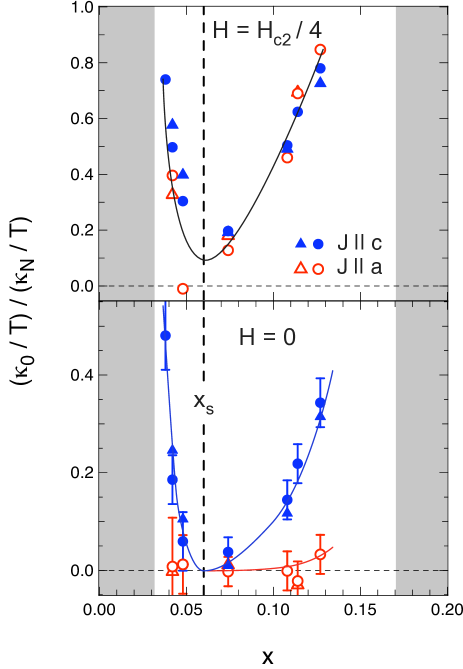
Figure 9: Residual linear term $\kappa_{0}/T$ of Co-Ba122 normalized by the normal-state value $\kappa_{\rm N}/T$ as a function of Co concentration $x$, at $H=0$ (lower panel) and at $H=H_{c2}/4$ (upper panel). Full blue symbols are for a heat current along the $c$ axis ($J~{}||~{}c$; circles for A samples, triangles for B samples in Table I). Empty red symbols are for a heat current along the $a$ axis ($J~{}||~{}a$; circles for A samples, triangles for B samples in Table II). The white interval between the two vertical grey bands at $x<0.032$ and $x>0.17$ is the region of superconductivity in the phase diagram (Fig. 1). The vertical dashed line at $x=0.06$ marks the approximate location of the critical doping $x_{s}$ where the structure at $T=0$ goes from orthorhombic (below) to tetragonal (above) Nandi2010 (see Fig. 1). Lines through the data points are a guide to the eye. Error bars on the $H=0$ data are shown for the A samples (circles).

IV.1 Gap nodes

IV.1.1 Zero magnetic field

Our central finding is the presence of a substantial residual linear term $\kappa_{0}/T$ in the thermal conductivity of Co-Ba122 in zero field, for heat transport along the $c$ axis. It implies the presence of nodes in the superconducting gap, such that $\Delta({\bf k})=0$ for some wavevectors ${\bf k}$ on the Fermi surface.Hirschfeld1988 ; Graf1996 ; Durst2000 ; Mishra2009 ; Shakeripour2009a Because heat conduction in a given direction is dominated by quasiparticles with ${\bf k}$ vectors along that direction,Hirschfeld1988 ; Graf1996 the fact that $\kappa_{0}/T$ is negligible when heat transport is along the $a$ axis, at all $x$, implies that the nodes are located in regions of the Fermi surface that contribute strongly to $c$-axis conduction but very little to in-plane conduction. The anisotropy of $\kappa_{0}/T$ becomes pronounced as $x$ moves away from the critical doping $x_{s}\simeq 0.06$, in either direction. For $x>0.06$, we see that the $a/c$ anisotropy in $\kappa_{0}/\kappa_{\rm N}$ is at least a factor 10 (see Fig. 9). Such a large anisotropy is not expected in a scenario of isotropic pair-breaking,Kogan2009 and it confirms that the residual linear term seen in the $c$ direction is due to nodes.

At the highest doping studied here, $x=0.127$, $\kappa_{0}/\kappa_{\rm N}=0.34\pm 0.03$ for $J~{}||~{}c$. (This is for sample A, which has the lowest $T_{c}$ in the overdoped regime; see Table I.) This magnitude is typical of superconductors with a line of nodes in the gap. In the heavy-fermion superconductor CeIrIn₅, with $T_{c}=0.4$ K and $H_{c2}\simeq 0.5$ T, $\kappa_{0}/\kappa_{\rm N}\simeq 0.2$.Shakeripour2007 ; Shakeripour2009 In the ruthenate superconductor Sr₂RuO₄, with $T_{c}=1.5$ K and $H_{c2}=1.5$ T, $\kappa_{0}/\kappa_{\rm N}\simeq 0.1-0.3$ (depending on sample purity).Suzuki2002 In the overdoped cuprate Tl₂Ba₂CuO_6-δ (Tl-2201), a $d$-wave superconductor with $T_{c}=15$ K and $H_{c2}\simeq 7$ T, $\kappa_{0}/\kappa_{\rm N}\simeq 0.35$.Proust2002 In the latter case, because the order parameter is well-known and the Fermi surface is very simple (a single 2D cylinder), it was possible to show that the magnitude of $\kappa_{0}/T$ agrees quantitatively with the theoretical BCS expression for the residual linear term in a $d$-wave superconductor,Hawthorn2007 namely $\kappa_{0}/T=(k^{2}_{\rm B}/3d)(k_{\rm F}v_{\rm F}/S)$,Graf1996 ; Durst2000 ; Shakeripour2009a where $d$ is the interlayer separation, $k_{\rm F}$ and $v_{\rm F}$ are the Fermi wavevector and velocity at the node, respectively, and $S\equiv\delta\Delta/\delta k$ is the slope of the gap at the node. (For a $d$-wave gap with $\Delta(k)=\Delta_{0}$cos($2\phi$), $S=2\Delta_{0}$.)

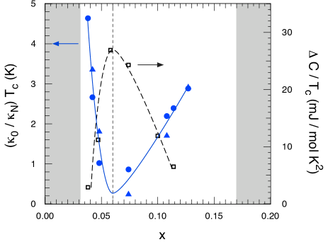
Figure 10: Comparison of heat transport by nodal quasiparticles and the jump in heat capacity at the superconducting transition, in Co-Ba122 as a function of Co concentration $x$. Heat transport is measured as the zero-field residual linear term in the thermal conductivity along the $c$ axis, $\kappa_{c0}/T$, normalized by the corresponding normal-state conductivity at $T\to 0$, $\kappa_{\rm cN}/T$, multiplied by $T_{c}$. The heat capacity jump $\Delta C$ is divided by $T_{c}$ (from Ref. Budko2009, ). The vertical dashed line marks the location of $x_{s}$. Other lines are a guide to the eye.

If the line of nodes in the gap is imposed by the symmetry of the order parameter, as in a $d$-wave state, then $\kappa_{0}/T$ is universal, i.e. independent of the impurity scattering rate $\Gamma_{0}$, in the clean limit $\hbar\Gamma_{0}<<\Delta_{0}$.Graf1996 ; Durst2000 Such universal transport was demonstrated experimentally for CeIrIn₅,Shakeripour2009 Sr₂RuO₄,Suzuki2002 and the cuprates YBa₂Cu₃O₇ Taillefer1997 and Bi₂Sr₂CaCu₂O₈.Nakamae2001 As a fraction of the normal-state conductivity, one then gets $(\kappa_{0}/T)/(\kappa_{\rm N}/T)\equiv\kappa_{0}/\kappa_{\rm N}\propto\hbar\Gamma_{0}/S$.Graf1996 However, if the nodes are not imposed by symmetry, but are ‘accidental’, as in an ‘extended-$s$-wave’ state, they still cause a non-zero residual linear term, with $\kappa_{0}/T\propto 1/S$, but $\kappa_{0}/T$ is no longer universal, because $S$ depends on the scattering rate $\Gamma_{0}$.Mishra2009

In Fig. 9, we see that $\kappa_{c0}/\kappa_{\rm cN}$ exhibits a striking U-shaped dependence on Co concentration $x$, with $\kappa_{c0}/\kappa_{\rm cN}\to 0$ as $x\to x_{s}$. Just above $x_{s}$, at $x=0.074$, $\kappa_{c0}/T=0.2\pm 0.5~{}\mu$W/K² cm. (This is for sample B, which is closest to $x_{s}$, as it has the highest $T_{c}$; see Table I.) This is equal to zero within error bars, indicating that there are no nodes in the gap at this concentration, as also inferred from the field dependence (see below). If the nodes can be removed simply by changing $x$, then these nodes must be accidental, not imposed by symmetry.

Given that the change in $\kappa_{0}/\kappa_{\rm N}$ with $x$ on the overdoped side is due to a change in $\kappa_{0}/T$ and not a change in $\kappa_{\rm N}/T$ (since $\rho_{0}$ is independent of $x$, within error bars), we attribute the dramatic rise in $\kappa_{0}/\kappa_{\rm N}$ from $x=0.074$ to $x=0.127$ to a decrease of the slope $S$ with increasing $x$. Part of this decrease must be due to a drop in the overall strength of superconductivity, as measured by the decreasing $T_{c}$. We can factor out that effect by multiplying $\kappa_{0}/\kappa_{\rm N}$ by $T_{c}$, as shown in Fig. 10. We see that $\kappa_{0}/\kappa_{\rm N}\times T_{c}$ vs $x$ is far from constant, as it would be if the decrease of $\Delta({\bf k})$ vs $x$ was uniform, independent of ${\bf k}$. In a $d$-wave superconductor, for example, $S$ would typically scale with the gap maximum $\Delta_{0}$, which itself would scale with $T_{c}$, giving a constant product $\kappa_{0}/\kappa_{\rm N}\times T_{c}$ (for a constant $\Gamma_{0}$). By contrast, in Co-Ba122 the slope of the gap at the nodes decreases faster than that part of the gap structure which controls $T_{c}$. In other words, $\Delta({\bf k})$ must be acquiring a stronger and stronger ${\bf k}$ dependence, or modulation, with increasing $x$.

In the underdoped regime, for samples with $x=0.048$ and lower, the metal is antiferromagnetic Fernandes2010 and its Fermi surface is reconstructed by the antiferromagnetic order. Nevertheless, a residual linear term $\kappa_{c0}/T$ is still observed at $H=0$ (see Fig. 9). At $x=0.038$, it is even larger than at $x=0.127$, namely $\kappa_{0}/\kappa_{N}=0.48\pm~{}0.04$ (see Table I). This implies that nodes are present in the superconducting gap inside the region of co-existing antiferromagnetic order. The fact that $\kappa_{0}/T$ is again strongly anisotropic (see Fig. 9) means that those nodes are still located in regions of the Fermi surface that contribute strongly to $c$-axis conduction and little to $a$-axis conduction. The fact that the nodes survive the Fermi-surface reconstruction is consistent with their location in regions with strong 3D character, since the spin-density wave gaps the nested portions of the Fermi surface, which are typically those with strong 2D character. (It should be emphasized that the mechanisms responsible for the drop in $T_{c}$ and the rise in $\kappa_{0}/\kappa_{\rm N}$ are likely to be different above and below optimal doping.)

IV.1.2 Field dependence

The effect of a magnetic field on $\kappa_{0}/T$ reveals how easy it is to excite quasiparticles at $T=0$.Shakeripour2009a ; Mishra2009 ; Kubert1998 For a gap with nodes, the rise in $\kappa_{0}/T$ with $H$ is very fast, because delocalized quasiparticles exist outside the vortices,Kubert1998 as shown for the $d$-wave superconductor Tl-2201 in Fig. 11. For a full gap without nodes or deep minima, such as in the $s$-wave superconductor Nb, the rise in $\kappa_{0}/T$ vs $H$ is exponentially slow (see Fig. 11), because it relies on tunneling between quasiparticle states localized on adjacent vortices. For Co-Ba122 at $x=0.127$, $\kappa_{c0}/\kappa_{\rm N}$ is seen to track the $d$-wave data all the way from $H=0$ to $H=H_{c2}$. This nicely confirms the presence of nodes in the gap structure of overdoped Co-Ba122 that dominate the transport along the $c$ axis.

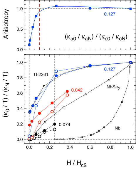
Figure 11: Bottom panel: Residual linear term $\kappa_{0}/T$ of Co-Ba122 normalized by the normal-state value $\kappa_{\rm N}/T$ as a function of magnetic field $H$, plotted as $(\kappa_{0}/T)/(\kappa_{\rm N}/T)\equiv\kappa_{0}/\kappa_{\rm N}$ vs $H/H_{c2}$ for three representative Co concentrations, as indicated: underdoped ($x=0.042$; red), slightly overdoped ($x=0.074$; black), and strongly overdoped ($x=0.127$; blue). $\kappa_{\rm N}/T$ is obtained from the Wiedemann-Franz law (see text and Tables I and II), except for the samples with $x=0.127$ where we use the value of $\kappa_{0}/T$ measured at $H=15$ T, since $H_{c2}=15$ T at that concentration. Full circles are for a heat current along the $c$ axis ($J~{}||~{}c$; data from three A samples - see Table I). Empty circles are for a heat current along the $a$ axis ($J~{}||~{}a$; data from three A samples - see Table II). The vertical dashed line marks $H=H_{c2}/4$; the value of $\kappa_{0}/\kappa_{\rm N}$ at $H_{c2}/4$ is plotted in the top panel of Fig. 9, for all $x$. We also reproduce corresponding data for the $d$-wave superconductor Tl-2201 (from Ref. Proust2002, ), the isotropic $s$-wave superconductor Nb, and the multi-band $s$-wave superconductor NbSe₂ (from Ref. Boaknin2003, ). Top panel: Anisotropy of the normalized residual linear term $\kappa_{0}/\kappa_{\rm N}$ at $x=0.127$. The red dashed line at $H_{c2}/10$ marks roughly the field beyond which $\kappa_{0}/\kappa_{\rm N}$ becomes isotropic.

By contrast, at $x=0.074$, the initial rise in $\kappa_{c0}/T$ vs $H$ has the positive (upwards) curvature typical of a nodeless gap, for both samples A and B (see Fig. 6). The rise at low $H$ is faster than in a simple $s$-wave superconductor like Nb (Fig. 11), either because of a $k$-dependence of the gap or because of a multi-band variation of the gap amplitude, or both. A multi-band variation is what causes the fast initial rise in $\kappa_{0}/T$ vs $H$ (with positive curvature) in NbSe₂ Boaknin2003 (see Fig. 11). This $H$ dependence strongly suggests that there are no nodes in the gap of Co-Ba122 at $x=0.074$, as inferred above from the negligible value of $\kappa_{a0}/T$.

IV.2 Gap minima

We saw that nodes in the gap have two general and related signatures in the thermal conductivity:Shakeripour2009a 1) a finite residual linear term $\kappa_{0}/T$ in zero field, and 2) a fast initial rise in $\kappa_{0}/T$ with $H$. Both signatures are clearly observed in Co-Ba122 at $x=0.127$ for $J~{}||~{}c$. For $J~{}||~{}a$, however, the situation is quite different. Indeed, $\kappa_{a0}/T$ is negligible at $H=0$, for all $x$, as also found in previous measurements of $\kappa_{a}$ on underdoped K-Ba122,Luo2009 optimally-doped Ni-Ba122,Ding2009 and overdoped Co-Ba122.Dong2010

Consequently, the fast initial rise in $\kappa_{0}/T$ with $H$ for $J~{}||~{}a$, seen in Fig. 11, is not due to nodes but rather to the presence of deep minima in the gap, in regions of the Fermi surface that contribute significantly to in-plane conduction, as previously reported.Tanatar2010 In the top panel of Fig. 9, we show the normalized residual linear term $\kappa_{0}/\kappa_{\rm N}$ measured at $H=H_{c2}/4$. We see that in the overdoped regime the $\kappa_{0}/\kappa_{\rm N}$ values are the same for both current directions, at all $x$. In other words, whereas $\kappa_{0}/\kappa_{\rm N}$ is very anisotropic at $H=0$, it is essentially isotropic at $H>H_{c2}/10$, as shown for $x=0.127$ in the top panel of Fig. 11. But quasiparticle transport for $J~{}||~{}c$ is due to nodal excitations, whereas quasiparticle transport for $J~{}||~{}a$ comes from field-induced excitations across a minimum gap. In a single-band model, say with a single ellipsoidal Fermi surface, this contrast between zero-field anisotropy and finite-field isotropy can only be described by invoking two unrelated features in the gap structure $\Delta({\bf k})$: nodes along the $c$ axis and deep minima in the basal plane. However, the fact that $\kappa_{0}/\kappa_{\rm N}$ remains isotropic at all $x$ (for $H=H_{c2}/4$) strongly suggests that nodes and minima are in fact intimately related. We therefore propose that they both come from the same tendency of the gap function $\Delta({\bf k})$ to develop a strong modulation as a function of ${\bf k}$, which causes a deep minimum on one Fermi surface and an even deeper minimum on another Fermi surface, where the gap would actually go to (or through) zero. In other words, instead of invoking two unrelated features of the gap structure on a single Fermi surface, we invoke a single property of the gap structure which leads to two related manifestations on separate Fermi surfaces.

IV.3 Two simple models for the gap structure

For the purpose of illustration, we consider a simplified two-band model for the Fermi surface, whereby one surface has strong 3D character and the other has quasi-2D character, as sketched in Fig. 12. The 3D Fermi surface can either be open along the $c$ axis, as drawn in Fig. 12 and suggested by some ARPES data,Malaeb2009 or closed, as suggested by some band structure calculations.Mazin2009 The 3D Fermi surface is responsible for most of the $c$-axis conduction and the 2D surface for most of the $a$-axis conduction (recall that in the $T=0$ limit $\kappa_{\rm aN}/\kappa_{\rm cN}=\rho_{\rm cN}/\rho_{\rm aN}\simeq 20$). Note that in reality the Fermi surface of Co-Ba122 contains at least four separate sheets;Mazin2009 ; Graser2010 our model requires that at least one of these has strong 3D character and it treats all others in terms of a single Fermi surface, the second quasi-2D sheet. We then propose that the gap $\Delta({\bf k})$ varies strongly as a function of ${\bf k}$, on both Fermi surface sheets. There are two basic scenarios: a gap modulation as a function of $k_{z}$, illustrated in Fig. 12, or a gap modulation as a function of the azimuthal angle $\phi$ in the basal plane, illustrated in Fig. 13. The strong modulation extends to negative values on the 3D Fermi surface, thereby producing nodes where $\Delta({\bf k})=0$, whereas it only produces a deep minimum (where $\Delta=\Delta_{\rm min}$) on the 2D Fermi surface (at least in the range of concentrations covered here). In the first scenario (Fig. 12), the lines of nodes are horizontal circular loops in a plane normal to the $c$ axis; in the second scenario (Fig. 13), they are vertical lines along the $c$ axis.

Both versions of the model explain the isotropy at $H_{c2}/4$ and the anisotropy at $H=0$. The isotropy of $\kappa_{0}/\kappa_{\rm N}$ follows fundamentally from having a similar ${\bf k}$ modulation of the gap on both Fermi surfaces. When the field is large enough to excite quasiparticles across the minimum gap on the 2D Fermi surface, quasiparticle transport from both Fermi surfaces will be similar, explaining the rapid and isotropic rise in $\kappa_{0}/T$ with $H$. By contrast, at $H=0$ no quasiparticles are excited on the 2D Fermi surface at $T=0$ (since $k_{\rm B}T<<\Delta_{\rm min}$), whereas nodal quasiparticles are always present on the 3D surface. This explains the large anisotropy of $\kappa_{0}/\kappa_{\rm N}$ at $H=0$. Note that this anisotropy is not governed by the anisotropy of the gap itself, i.e. by the direction of the gap modulation, but rather by the fact that the nodes lie on the 3D Fermi surface. (Whether horizontal or vertical line nodes are more consistent with our data depends on details of the real Fermi surface of Co-Ba122.) The nodal quasiparticles on the 3D sheet must also contribute to $a$-axis conduction. Assuming that for the 3D Fermi surface $\kappa_{a0}/T\simeq\kappa_{c0}/T$ at $H=0$, we should detect a residual linear term $\kappa_{a0}/T\simeq 6~{}\mu$W/K² cm in the $a$-axis sample with $x=0.127$, for example. This is indeed consistent, within error bars, with the value we extrapolate for the $a$-axis data at $x=0.127$ (Fig. 7), namely $\kappa_{a0}/T=17~{}\pm~{}20~{}\mu$W/K² cm (Table II).

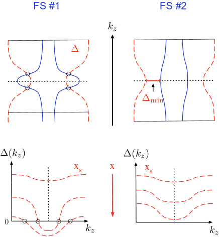
Figure 12: First model for the gap structure. Simplified two-band model of the Fermi surface of Co-Ba122 (blue solid line), shown in the $a-c$ plane, with $k_{z}~{}||~{}c$ in the vertical direction. Although in reality the Fermi surface of Co-Ba122 consists of at least four sheets, in our model we reduce it to two sheets: a sheet with strong 3D character (FS $\#$ 1; top left) and a sheet with quasi-2D character (FS $\#$2; top right). The superconducting gap $\Delta({\bf k})$ on both Fermi surfaces (red dashed line) varies strongly as a function of $k_{z}$, as shown on the bottom for three representative concentrations $x$ from $x_{s}$ upwards. On the 3D Fermi surface ($\#$1), the gap modulation is such that it extends to negative values, producing nodes (black circles) at certain points. On the 2D Fermi surface ($\#$2), the gap modulation is strong enough to cause a deep minimum (where $\Delta=\Delta_{\rm min}$), but not nodes. At $x=x_{s}$, the gap minima are shallow and there are no nodes on either Fermi surface. With increasing $x$ (decreasing $T_{c}$), the modulation increases, the minima deepen and the nodes appear. A further increase in $x$ (beyond the maximal concentration in this study) could eventually also yield nodes on FS $\#$2.

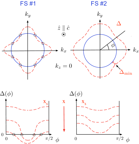
Figure 13: Second model for the gap structure. Same as in Fig. 12, except that the modulation of the superconducting gap $\Delta({\bf k})$ is now a function of the azimuthal angle $\phi$ in the basal plane.

In both versions of our model for the gap structure, the U-shaped $x$ dependence of $\kappa_{0}/\kappa_{\rm N}$ is attributed to an increase in the modulation of the gap as $x$ moves away from $x_{s}$, as illustrated in Figs. 12 and  13. The fact that the U-shaped curves in Fig. 9 have their minimum where the (inverted U-shaped) $T_{c}$ vs $x$ curve has its maximum points to a reverse correlation between $T_{c}$ and gap modulation. Modulation is a sign of weakness. The presence of nodes in the gap may then be an indicator that pairing conditions are less than optimal.

It is possible that at high enough $x$ in the overdoped regime $\Delta_{\rm min}$, the minimum value of the gap on the quasi-2D Fermi surface, goes to zero, so that nodes appear on that Fermi surface as well. This would immediately cause $\kappa_{a0}/T$ to become sizable. It is conceivable that the large value of $\kappa_{a0}/T$ measured in undoped KFe₂As₂,Dong2010a which can be viewed as the strong doping limit of K-Ba122, is the result of a gap modulation so strong that it goes to (through) zero on all Fermi surfaces.

A pronounced modulation of $\Delta({\bf k})$ should manifest itself in a number of physical properties. For example, in an $s$-wave superconductor, a variation of the gap magnitude over the Fermi surface, whether from band to band as in MgB₂,Bouquet2002 or from ${\bf k}$ dependence (anisotropy) as in Zn, Gubser1973 leads to a suppressed ratio of specific heat jump $\Delta C$ at the transition to $T_{c}$. The pronounced gap modulation and anisotropy revealed by the thermal conductivity could therefore account for the dramatic variation of $\Delta C/T_{c}$ measured in Co-Ba122 vs $x$,Budko2009 reproduced in Fig. 10. $\Delta C/T_{c}$ is seen to be maximal where $\kappa_{0}/\kappa_{\rm N}$ is minimal, i.e. where the gap modulation is weakest, and it drops just as rapidly with a change in $x$ as $\kappa_{0}/\kappa_{\rm N}$ rises.

IV.4 Theoretical calculations

The two-band picture suggested by our thermal conductivity data is reminiscent of the proximity scenario proposed for the three-band quasi-2D $p$-wave superconductor Sr₂RuO₄,Zhitomirsky2001a where superconductivity originates on one band, the most 2D one, and is induced by proximity on the other two bands. This $k$-space promixity effect is such that a $k_{z}$ modulation of the induced gap produces horizontal line nodes on the latter two Fermi surfaces,Zhitomirsky2001a in analogy with the horizontal-line scenario of Fig. 12. A proximity scenario of this sort was in fact proposed for the pnictides,Laad2009 predicting $c$-axis nodes in the superconducting gap. The effect on the superconducting gap structure of including the $k_{z}$ dispersion of the Fermi surface in BaFe₂As₂ was recently calculated within a spin-fluctuation pairing mechanism on a 3D multi-orbital Fermi surface.Graser2010 A strong modulation of the gap $\Delta({\bf k})$ as a function of both $k_{z}$ and $\phi$ is obtained which can indeed, for some parameters, lead to accidental nodes.

The thermal conductivity of pnictides was calculated in a 2D two-band model for the case of an extended-$s$-wave gap (of $A_{1g}$ symmetry).Mishra2009 These calculations show that the presence of deep minima in the gap, in this case as a function of $\phi$, can account for the rapid initial rise observed in $\kappa_{a0}/T$ vs $H$, starting from $\kappa_{a0}/T=0$ at $H=0$. It seems clear that calculations for a gap whose deep minima occur instead as a function of $k_{z}$ would yield similar results. It will be interesting to see what calculations of the thermal conductivity give when applied to the 3D model of Ref. Graser2010, , or indeed to the simple two-band models proposed here (in Figs. 12 and 13).

V Conclusions

In summary, our measurements of the thermal conductivity in the iron-arsenide superconductor Ba(Fe_1-xCo_x)₂As₂ show unambiguously that the gap $\Delta({\bf k})$ has nodes. These nodes are present in both the overdoped and the underdoped regions of the phase diagram, implying that they survive the Fermi-surface reconstruction provoked by the antiferromagnetic order in the underdoped region. The nodes are located in regions of the Fermi surface that dominate $c$-axis conduction and contribute very little to in-plane conductivity. The fact that the strongly anisotropic quasiparticle transport at $H=0$ becomes isotropic in a magnetic field $H=H_{c2}/4$ shows that there must be a deep minimum in the gap in regions of the Fermi surface that dominate in-plane transport. These two features - nodes on 3D regions and minima on 2D regions of the Fermi surface - point to a strong modulation of the gap as a function of ${\bf k}$. This modulation of $\Delta({\bf k})$ would be present on all Fermi surfaces, but be most pronounced on that surface with strongest $k_{z}$ dispersion, where it has nodes. This suggests a close relation between the 3D character of the Fermi surface and gap modulation.

The anisotropy of $\kappa$ shows a strong evolution with Co concentration $x$. At optimal doping, where $T_{c}$ is maximal, there are no nodes and $\kappa_{0}/T$ has the anisotropy of the normal state. With increasing $x$, nodes appear and $\kappa_{0}/T$ acquires a strong anisotropy. We attribute this to an increase in the gap modulation with $x$, which may explain the strong decrease in the specific heat jump at $T_{c}$ Budko2009 and the change in the power-law temperature dependence of the penetration depth.Gordon2009a ; Gordon2009 The fact that nodes are located in regions that dominate $c$-axis conduction is consistent with the fact that the penetration depth along the $c$ axis has a linear temperature dependence.Martin2010

Horizontal line nodes in Co-Ba122, which would be the result of a strong modulation of the gap along $k_{z}$ rather than a strong in-plane angular dependence, would reconcile the isotropic azimuthal angular dependence of the gap seen by ARPES with the evidence of nodes or minima from thermal conductivity, NMR relaxation rate and penetration depth measurements in Co-Ba122 and other iron-based superconductors. A $k_{z}$ modulation of $\Delta({\bf k})$ should be detectable by ARPES, especially in the overdoped regime where it would be strongest.

Because the nodes go away by tuning $x$ towards optimal doping, we infer that they are ‘accidental’, i.e. not imposed by symmetry, and so consistent a priori with any superconducting order parameter, including the $s_{\pm}$ state.Mazin2008 ; Kuroki2008 ; Vorontsov2008 Although accidental nodes are not a direct signature of the symmetry, the strong modulation of the gap nevertheless reflects an underlying ${\bf k}$ dependence of the pairing interaction, and as such the 3D character of the gap function $\Delta({\bf k})$ is an important element in understanding what controls $T_{c}$ in this family of superconductors.

VI Acknowledgements

We thank P. J. Hirschfeld, V. G. Kogan, P. A. Lee, I. I. Mazin, S. Sachdev and T. Senthil for fruitful discussions, and J. Corbin for his assistance with the experiments. Work at the Ames Laboratory was supported by the US Department of Energy, Office of Basic Energy Sciences under Contract No. DE-AC02-07CH11358. R. P. acknowledges support from the Alfred P. Sloan Foundation. L. T. acknowledges support from the Canadian Institute for Advanced Research and funding from NSERC, CFI, FQRNT and a Canada Research Chair.

References

- (1) Y. Kamihara, T. Watanabe, M. Hirano, and H. Hosono, J. Amer. Chem. Soc. 130, 3296 (2008).
- (2) Z.-A. Ren, W. Lu, J. Yang, W. Yi, X.-L. Shen, Z.-C. Li, G.-C. Che, X.-L. Dong, L.-L. Sun, F. Zhou, and Z.-X. Zhao Chin. Phys. Lett. 25, 2215 (2008).
- (3) K. Ishida, Y. Nakai, and H. Hosono, J. Phys. Soc. Jpn. 78, 062001 (2009).
- (4) I. I. Mazin, Nature 464, 183 (2010).
- (5) P. L. Alireza, Y. T. C. Ko, J. Gillett, C. M. Petrone, J. M. Cole, G. G. Lonzarich, and S. E. Sebastian, J. Phys: Condens. Matter 21, 012208 (2009).
- (6) M. Rotter, M. Tegel, and D. Johrendt, Phys. Rev. Lett. 101, 107006 (2008).
- (7) A. S. Sefat, R. Jin, M. A. McGuire, B. C. Sales, D. J. Singh, and D. Mandrus, Phys. Rev. Lett. 101, 117004 (2008).
- (8) N. Ni, M. E. Tillman, J.-Q. Yan, A. Kracher, S. T. Hannahs, S. L. Bud’ko, and P. C. Canfield, Phys. Rev. B 78, 214515 (2008).
- (9) S. Nandi, M. G. Kim, A. Kreyssig, R. M. Fernandes, D. K. Pratt, A. Thaler, N. Ni, S. L. Bud’ko, P. C. Canfield, J. Schmalian, R. J. McQueeney, and A. I. Goldman, Phys. Rev. Lett. 104, 057006 (2010).
- (10) R. M. Fernandes, D. K. Pratt, W. Tian, J. Zarestky, A. Kreyssig, S. Nandi, M. G. Kim, A. Thaler, N. Ni, P. C. Canfield, R. J. McQueeney, J. Schmalian, and A. I. Goldman, Phys. Rev. B 81, 140501 (2010).
- (11) K. Nakayama, T. Sato, P. Richard, Y.-M. Xu, Y. Sekiba, S. Souma, G. F. Chen, J. L. Luo, N. L. Wang, H. Ding, and T. Takahashi, Europhys. Lett. 85, 67002 (2009).
- (12) K. Terashima, Y. Sekiba, J. H. Bowen, K. Nakayama, T. Kawahara, T. Sato, P. Richard, Y.-M. Xu, L. J. Li, G. H. Cao, Z.-A. Xu, H. Ding, and T. Takahashi, Proc. Natl. Acad. Sci. U.S.A. 106, 7330 (2009).
- (13) P. Samuely, Z. Pribulova, P. Szabo, G. Pristas, S. L. Bud’ko, and P. C. Canfield, Physica C 469, 507 (2009).
- (14) Y.-M. Xu, P. Richard, K. Nakayama, T. Kawahara, Y. Sekiba, T. Qian, M. Neupane, S. Souma, T. Sato, T. Takahashi, H. Luo, H.-H. Wen, G.-F. Chen, N.-L. Wang, Z. Wang, Z. Fang, X. Dai, and H. Ding, arXiv: 0905.4467.
- (15) I. I. Mazin, D. J. Singh, M. D. Johannes, and M. H. Du, Phys. Rev. Lett. 101, 057003 (2008).
- (16) K. Kuroki, S. Onari, R. Arita, H. Usui, Y. Tanaka, H. Kontani, and H. Aoki, Phys. Rev. Lett. 101, 087004 (2008).
- (17) A. B. Vorontsov, M. G. Vavilov, and A. V. Chubukov, Phys. Rev. B 79, 060508 (2008).
- (18) R. T. Gordon, N. Ni, C. Martin, M. A. Tanatar, M. D. Vannette, H. Kim, G. D. Samolyuk, J. Schmalian, S. Nandi, A. Kreyssig, A. I. Goldman, J. Q. Yan, S. L. Bud’ko, P. C. Canfield, and R. Prozorov, Phys. Rev. Lett. 102, 127004 (2009).
- (19) R. T. Gordon, C. Martin, H. Kim, N. Ni, M. A. Tanatar, J. Schmalian, I. I. Mazin, S. L. Bud’ko, P. C. Canfield, and R. Prozorov Phys. Rev. B 79, 100506 (R) (2009).
- (20) H. Fukazawa, Y. Yamada, K. Kondo, T. Saito, Y. Kohori, K. Kuga, Y. Matsumoto, S. Nakatsuji, H. Kito, P. M. Shirage, K. Kihou, N. Takeshita, C.-H. Lee, A. Iyo, and H. Eisaki, J. Phys. Soc. Jpn. 78, 033704 (2009).
- (21) X. G. Luo, M. A. Tanatar, J.-Ph. Reid, H. Shakeripour, N. Doiron-Leyraud, N. Ni, S. L. Bud’ko, P. C. Canfield, H. Luo, Z. Wang, H.-H. Wen, R. Prozorov, and L. Taillefer, Phys. Rev. B 80, 140503 (R) (2009).
- (22) M. A. Tanatar, J.-Ph. Reid, H. Shakeripour, X. G. Luo, N. Doiron-Leyraud, N. Ni, S. L. Bud’ko, P. C. Canfield, R. Prozorov, and L. Taillefer, Phys. Rev. Lett. 104, 067002 (2010).
- (23) J. K. Dong, S. Y. Zhou, T. Y. Guan, X. Qiu, C. Zhang, P. Cheng, L. Fang, H. H. Wen, and S. Y. Li, Phys. Rev. B 81, 094520 (2010).
- (24) C. Martin, H. Kim, R. T. Gordon, N. Ni, V. G. Kogan, S. L. Bud’ko, P. C. Canfield, M. A. Tanatar, and R. Prozorov, Phys. Rev. B 81, 060505 (2010).
- (25) W. Malaeb, T. Yoshida, A. Fujimori, M. Kubota, K. Ono, K. Kihou, P. M. Shirage, H. Kito, A. Iyo, H. Eisaki, Y. Nakajima, T. Tamegai, and R. Arita, J. Phys. Soc. Jpn. 78, 123706 (2009).
- (26) C. Utfeld, J. Laverock, T. D. Haynes, S. B. Dugdale, J. A. Duffy, M. W. Butchers, J. W. Taylor, S. R. Giblin, J. G. Analytis, J. Chu, I. R. Fisher, M. Itou, and Y. Sakurai, Phys. Rev. B 81, 064509 (2010).
- (27) A. F. Kemper, C. Cao, P. J. Hirschfeld, and H.-P. Cheng, Phys. Rev. B 80, 104511 (2009).
- (28) J. G. Analytis, R. D. McDonald, J.-H. Chu, S. C. Riggs, A. F. Bangura, C. Kucharczyk, M. Johannes, and I. R. Fisher, Phys. Rev. B 80, 064507 (2009).
- (29) M. A. Tanatar, N. Ni, C. Martin, R. T. Gordon, H. Kim, V. G. Kogan, G. D. Samolyuk, S. L. Bud ko, P. C. Canfield, and R. Prozorov, Phys. Rev. B 79, 094507 (2009).
- (30) M. A. Tanatar, N. Ni, G. D. Samolyuk, S. L. Bud’ko, P. C. Canfield, and R. Prozorov, Phys. Rev. B 79, 134528 (2009).
- (31) M. S. Laad and L. Craco, Phys. Rev. Lett. 103, 017002 (2009).
- (32) S. Graser, A. F. Kemper, T. A. Maier, H.-P. Cheng, P. J. Hirschfeld, and D. J. Scalapino, arXiv:1003.0133.
- (33) S. Chi, A. Schneidewind, J. Zhao, L. W. Harriger, L. Li, Y. Luo, G. Cao, Z. Xu, M. Loewenhaupt, J. Hu, and P. Dai, Phys. Rev. Lett. 102, 107006 (2009).
- (34) P. J. Hirschfeld, P. Wolfle, and D. Einzel, Phys. Rev. B 37, 83 (1988).
- (35) M. J. Graf, S.-K. Yip, J. A. Sauls, and D. Rainer, Phys. Rev. B 53, 15147 (1996).
- (36) A. C. Durst and P.A. Lee, Phys. Rev. B 62, 1270 (2000).
- (37) L. Taillefer, B. Lussier, R. Gagnon, K. Behnia, and H. Aubin, Phys. Rev. Lett. 79, 483 (1997).
- (38) M. Suzuki, M. A. Tanatar, N. Kikugawa, Z. Q. Mao, Y. Maeno, and T. Ishiguro, Phys. Rev. Lett. 88, 227004 (2002).
- (39) H. Shakeripour, C. Petrovic, and L. Taillefer, New J. Phys. 11, 055065 (2009).
- (40) H. Shakeripour, M. A. Tanatar, S. Y. Li, C. Petrovic, and L. Taillefer, Phys. Rev. Lett. 99, 187004 (2007).
- (41) M. Kano, Y. Kohama, D. Graf, F. Balakirev, A. S. Sefat, M. A. Mcguire, B. C. Sales, D. Mandrus, and S. W. Tozer, J. Phys. Soc. Jpn. 78, 084719 (2009).
- (42) M. Sutherland, D. G. Hawthorn, R. W. Hill, F. Ronning, S. Wakimoto, H. Zhang, C. Proust, E. Boaknin, C. Lupien, L. Taillefer, R. Liang, D. A. Bonn, W. N. Hardy, R. Gagnon, N. E. Hussey, T. Kimura, M. Nohara, and H. Takagi, Phys. Rev. B 67, 174520 (2003).
- (43) M. A. Tanatar, N. Ni, S. L. Bud’ko, P. C. Canfield, and R. Prozorov, Supercond. Sci. Technol. (to be published).
- (44) D. G. Hawthorn, S. Y. Li, M. Sutherland, E. Boaknin, R. W. Hill, C. Proust, F. Ronning, M. A. Tanatar, J. Paglione, and L. Taillefer, Phys. Rev. B 75, 104518 (2007).
- (45) S. Y. Li, J.-B. Bonnemaison, A. Payeur, P. Fournier, C. H. Wang, X. H. Chen, and L. Taillefer, Phys. Rev. B 77, 134501 (2008).
- (46) L. Ding, J. K. Dong, S. Y. Zhou, T. Y. Guan, X. Qiu, C. Zhang, L. J. Li, X. Lin, G. H. Cao, Z. A. Xu, and S. Y. Li, New J. Phys. 11, 093018 (2009).
- (47) V. Mishra, A. Vorontsov, P. J. Hirschfeld, and I. Vekhter, Phys. Rev. B 80, 224525 (2009).
- (48) V. G. Kogan, Phys. Rev. B 80, 214532 (2009),
- (49) H. Shakeripour, M. A. Tanatar, C. Petrovic, and L. Taillefer, arXiv:0902.1190.
- (50) C. Proust, E. Boaknin, R.W. Hill, L. Taillefer, and A. P. Mackenzie, Phys. Rev. Lett. 89, 147003 (2002).
- (51) S. L. Bud’ko, N. Ni, and P. C. Canfield, Phys. Rev. B 79, 220516 (2009).
- (52) S. Nakamae, K. Behnia, L. Balicas, F. Rullier-Albenque, H. Berger, and T. Tamegai, Phys. Rev. B 63, 184509 (2001).
- (53) C. Kubert and P. J. Hirschfeld, Phys. Rev. Lett. 80, 4963 (1998).
- (54) E. Boaknin, M. A. Tanatar, J. Paglione, D. G. Hawthorn, F. Ronning, R. W. Hill, M. Sutherland, L. Taillefer, J. Sonier, S. M. Hayden, and J. W. Brill, Phys. Rev. Lett. 90, 117003 (2003).
- (55) J. K. Dong, S. Y. Zhou, T. Y. Guan, H. Zhang, Y. F. Dai, X. Qiu, X. F. Wang, Y. He, X. H. Chen, and S. Y. Li, Phys. Rev. Lett. 104, 087005 (2010).
- (56) F. Bouquet, Y. Wang, I. Sheikin, T. Plackowski, A. Junod, S. Lee, and S. Tajima, Phys. Rev. Lett. 89, 257001 (2002).
- (57) D. U. Gubser and J. E. Cox, Phys. Rev. B 7, 4118 (1973).
- (58) I. I. Mazin and J. Schmalian, Physica C 469, 614 (2009).
- (59) M. E. Zhitomirsky and T. M. Rice, Phys. Rev. Lett. 87, 057001 (2001).