Shock waves in strongly coupled plasmas

Sergei Khlebnikov, Martin Kruczenski and Georgios Michalogiorgakis

Department of Physics, Purdue University
525 Northwestern Avenue, West Lafayette, IN 47907

skhleb@physics.purdue.edu  markru@purdue.edu  gmichalo@purdue.edu

Shock waves are supersonic disturbances propagating in a fluid and giving rise to dissipation and drag. Weak shocks, i.e., those of small amplitude, can be well described within the hydrodynamic approximation. On the other hand, strong shocks are discontinuous within hydrodynamics and therefore probe the microscopics of the theory. In this paper we consider the case of the strongly coupled $\mathcal{N}=4$ plasma whose microscopic description, applicable for scales smaller than the inverse temperature, is given in terms of gravity in an asymptotically $AdS_{5}$ space. In the gravity approximation, weak and strong shocks should be described by smooth metrics with no discontinuities. For weak shocks we find the dual metric in a derivative expansion and for strong shocks we use linearized gravity to find the exponential tail that determines the width of the shock. In particular we find that, when the velocity of the fluid relative to the shock approaches the speed of light $v\rightarrow 1$ the penetration depth $\ell$ scales as $\ell\sim(1-v^{2})^{1/4}$. We compare the results with second order hydrodynamics and the Israel-Stewart approximation. Although they all agree in the hydrodynamic regime of weak shocks, we show that there is not even qualitative agreement for strong shocks. For the gravity side, the existence of shock waves implies that there are disturbances of constant shape propagating on the horizon of the dual black holes.

1 Introduction and summary

The AdS/CFT correspondence [1, 2, 3, 4] realizes in practice the idea of describing gauge theories in terms of strings [5] and provides a new tool to study gauge theories at strong coupling. Recently, motivated by experimental and theoretical work on heavy ion collisions at RHIC, there was a wave of interest in using AdS/CFT to study the dynamics of strongly coupled plasmas, for a review see [6, 7, 8, 9, 10] and references therein. The main initial focus was on the low viscosity of the fluid and the drag force experienced by a quark moving through the plasma. More generically, in conformal plasmas, such as the one studied in AdS/CFT, the hydrodynamic description of the theory is valid up to length scales of order of the inverse temperature. Below that scale standard hydrodynamics breaks down, and we need to resort to the dual gravity description, which does not break down until the (much smaller) bulk string scale is reached. Alternative descriptions that are not based directly on microscopics, such as the Israel-Stewart theory, can be tested by comparison with the microscopic theory provided by the dual gravity.

In the present paper, we focus on a particular phenomenon in fluid dynamics, namely, shock waves. These are supersonic disturbances that propagate in the fluid and are typically produced by an object moving supersonically in the fluid or by a localized release of energy such as in explosions or collisions. In ideal fluids they are described by a surface of discontinuity where the normal velocity and the pressure have a jump. In the frame where the shock is at rest, the fluid goes from supersonic to subsonic, with the kinetic energy of the fluid converted into pressure and heat. This process is irreversible and generates entropy. In fact, it is the only dissipative mechanism in the case of strictly ideal fluids. In practice, of course, the fluid is never ideal so at small scales the viscosity also causes dissipation. If the shock wave is produced by an object moving in the fluid it also generates drag. Away from the shock the hydrodynamic approximation is good and allows to compute the jumps in velocity and pressure by using the conservation of energy (and other charges) across the shock. However in the region of discontinuity the gradients are in general large and a microscopic theory is necessary to have an appropriate description. In fact this breakdown of hydrodynamics is the reason why dissipation occurs in shock waves even for ideal fluids. For that reason, shock waves are not only phenomenologically interesting but, on the theoretical side, can be considered as a useful probe of the system. In practice, they are usually studied in non-relativistic systems and in fluids such as air and water. The relativistic case is of interest in astrophysics and in particular in heavy ion physics, which is the system closest to the one studied in this paper.

In the context of heavy ion physics there are different situations where shock waves can appear. One is during the period of the creation of the Quark Gluon Plasma. A simple model of particle production which gives reasonable results is Landau’s hydrodynamic model [11]. This model assumes that the fluid thermalizes instantaneously and then evolves according to ideal hydrodynamics. All the entropy is created at the initial stage as a result of the thermalization process. In a purely ideal hydrodynamical model the entropy can be generated only from shock waves which would therefore play an important role. However, initially the quark gluon plasma is far from equilibrium and therefore a hydrodynamical approximation might not be valid.

Within AdS/CFT entropy production in a heavy ion collision has been studied in [12] where two shock waves moving at the speed of light collide creating trapped surfaces. Also, [13] study the problem of reconstructing the bulk metric from the boundary. Several other aspects are examined in [14, 15]. Related work on gravitational shock waves appears in [16, 17, 18, 19, 20, 21, 22, 23, 24, 25].

Another instance where shock waves might appear in heavy ion collisions is the process where a hard parton moves through the plasma. The hard parton can be a heavy quark, a meson or a gluon. Calculations in AdS/CFT [26, 27, 28, 29, 30] show that there is a Mach cone created. That is, the energy density of the wave is concentrated in a angle close to the Mach angle. This is highly suggestive of the formation of a shock wave that cannot be described by the linearized approximations used in previous calculations. The real space profile of the stress energy tensor of a moving quark, calculated in [27] also supports the idea. Independently from AdS/CFT the possibility of shock waves in heavy ion collisions has been explored both theoretically and experimentally in [31, 32, 33, 34, 35, 36, 37, 38, 39, 40, 41, 42, 43, 44, 45, 46, 47, 48].

2 Shock waves in hydrodynamics

Figure 1: A supersonic flow reaches a fixed object creating a stationary shock wave. In heavy ion physics this scenario might be realized by a heavy parton moving through the plasma as suggested by the existence of a Mach cone.

Hydrodynamics can be used to study the region away form the shock where the gradients are small. For weak shocks, i.e., those of small amplitude, a hydrodynamic approximation that includes viscosity resolves the discontinuity and provides a smooth description of the shock wave. This can be corrected at higher orders in gradients if so desired. In this section we start by considering the ideal fluid case for arbitrary shocks and then the higher order hydrodynamic approximation for weak shocks. We also analyze the Israel-Stewart theory to compare later with the microscopic results.

2.1 Ideal Hydrodynamics

Ideal hydrodynamics is valid far from the shock and determines the main properties of shock waves. These are well known [49] and we describe them in this subsection as applied to our particular fluid. In relativistic ideal hydrodynamics the energy momentum tensor is given by

$${T^{\mu\nu}=p\eta^{\mu\nu}+\left(p+\rho\right)u^{\mu}u^{\nu}\;,\quad}$$

(1)

where $p$ is the pressure, $\rho$ the energy density and $u^{\mu}$ the four velocity of the fluid. The equations of motion are given by conservation of $T^{\mu\nu}$,

$$\partial_{\mu}T^{\mu\nu}=0\;,$$ (2)

and the equation of state, which for the strongly coupled $\mathcal{N}=4$ plasma is dictated by conformality and reads

$${\rho=3p=3(\pi T)^{4}\;.}$$

(3)

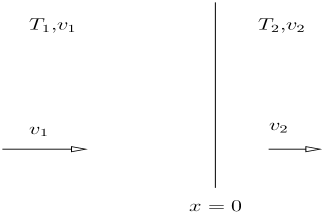
For a shock wave with a planar front, located for convenience at $x=0$, both $T^{tx}$ and $T^{xx}$ are constant throughout the fluid:

$${T^{tx}=4pu^{t}u^{x}=4p\frac{v}{1-v^{2}}\;,}$$

(4)

$${T^{xx}=p\left(1+4u_{x}^{2}\right)=p\frac{1+3v^{2}}{1-v^{2}}\;.}$$

(5)

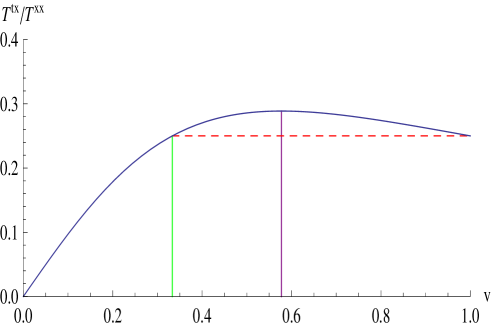
The possibility of a shock wave arises because there are different values of pressure and velocity that give the same value of $T^{tx}$ and $T^{xx}$. For example, the ratio $T^{tx}/T^{xx}$ depends only on the velocity and, as is seen from the plot in fig.(3) different velocities can give the same ratio $T^{tx}/T^{xx}$. More precisely, if we take that for $x\rightarrow-\infty$, $v=v_{1}$ and $T=T_{1}$ and for $x\rightarrow\infty$, $v=v_{2}$ and $T=T_{2}$ we can ensure that $T^{tx}$ and $T^{xx}$ are constant by imposing

$${v_{2}=\frac{1}{3v_{1}}\;,\quad p_{2}=p_{1}\frac{9v_{1}^{2}-1}{3(1-v_{1}^{2})}\;,\quad T_{2}=T_{1}\left(\frac{9v_{1}^{2}-1}{3(1-v_{1}^{2})}\right)^{1/4}\;.}$$

(6)

A particular case is $v_{1}=v_{2}=v_{s}$ where $v_{s}=\frac{1}{\sqrt{3}}$ is the speed of sound. In that case the jumps in $v$ and $T$ vanish. In general we have

$$1>v_{1}>\frac{1}{\sqrt{3}}>v_{2}>\frac{1}{3}$$ (7)

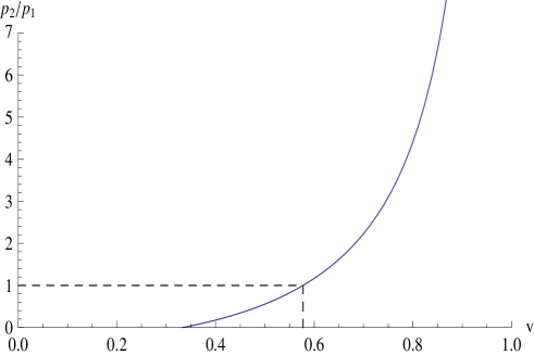
as can be seen from the relation $v_{1}v_{2}=\frac{1}{3}$. In particular, if $v_{2}=1/3$ on one side of the shock, the fluid on the other side moves at the speed of light. In principle, the conservation laws allow one to switch the values of the velocity between the front and back of the shock, i.e., take $v_{1}<v_{s}$ and $v_{2}>v_{s}$, but such solution would convert thermal energy into kinetic energy violating the second law of thermodynamics. In figure (4) we show the ratio of the pressures on the two sides. The supersonic side of the shock has a lower pressure which goes to zero when $v_{1}$ approaches one.

Figure 2: Sketch of a shock wave in the rest frame of the interface. For ideal hydrodynamics there is a discontinuity at $x=0$. Including the higher order terms in the expression of the stress energy tensor resolves the discontinuity. The conventions of the paper are that the fluid moves to the right. The left hand side is supersonic and the right hand side is subsonic since the opposite configuration violates the second law of thermodynamics.

For an object moving through the fluid this has the effect of changing the pressure that the object experiences. Indeed, defining the projector perpendicular to $u^{\mu}$ as $P^{\mu\nu}=\eta^{\mu\nu}+u^{\mu}u^{\nu}$ we obtain, from eq.(1):

$$P_{\mu\nu}\partial_{\alpha}T^{\alpha\nu}=0,\ \ \ \Rightarrow\ \ \ \ \partial_{\mu}T+u^{\nu}\partial_{\nu}\left(Tu_{\mu}\right)=0$$ (8)

For a stationary solution, taking the $\mu=0$ component we obtain:

$$u^{i}\partial_{i}\left(\gamma T\right)=0$$ (9)

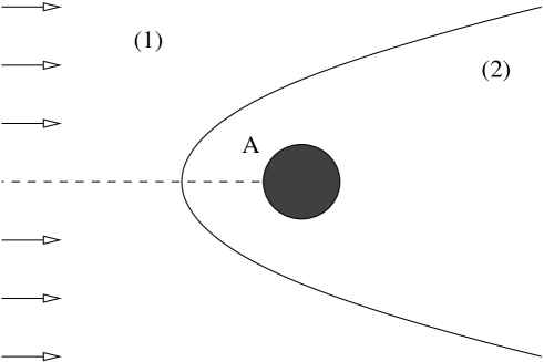
after replacing $u^{0}=\gamma$, where $\gamma$ is the Lorentz factor. We see that $\gamma T$ is conserved along a streamline. In particular for a situation as in fig.1 we can follow a streamline from infinity to the point $A$ and obtain, with and without a shock wave, the pressure:

$$p_{A}^{\mbox{(shock)}}=\gamma_{2}^{4}\,p_{2}=\frac{27v_{\infty}^{4}}{(9v_{\infty}^{2}-1)(1-v_{\infty}^{2})}p_{\infty},\ \ \ \ \ p_{A}^{\mbox{(no shock)}}=\gamma_{\infty}^{4}\,p_{\infty}=\frac{p_{\infty}}{(1-v_{\infty}^{2})^{2}}\;,$$ (10)

where we have used eq.(3) and the matching conditions (6) for the pressure and velocity across the shock wave.

Another interesting aspect of shock waves is the entropy production that is associated with them. In ideal hydrodynamics the entropy current is given by

$${s_{\mu}=4\pi^{4}T^{3}u_{\mu}\;,}$$

(11)

where we have chosen the normalization to give the entropy density of a fluid at rest. The difference between $s^{0}$ on the two sides of the shock is given by

$${\Delta s^{0}}$$

(12)

The entropy production comes from the difference of the two fluxes

$${\Delta s^{x}=s^{x}_{subsonic}-s^{x}_{supersonic}=\frac{4\pi^{2}T_{1}^{3}}{\sqrt{1-v_{1}^{2}}}\left(3^{-3/4}\left(\frac{9v_{1}^{2}-1}{1-v_{1}^{2}}\right)^{1/4}-v_{1}\right)\;.}$$

(13)

Kinetic energy from the supersonic side is transformed into thermal energy in the subsonic side and this creates entropy. Notice also that the ideal hydro is correct far from the shock, so this calculation gives the correct entropy production even if the fluid is not ideal.

Figure 3: The ratio $T^{tx}/T^{xx}$ for different velocities. For $v_{1}>\frac{1}{3}$ the equation $T^{tx}/T^{xx}=const.$ has two solutions and hence allows for a jump in velocity. When $v_{1}=\frac{1}{\sqrt{3}}$ there is no jump.

Figure 4: The ratio of pressure for the two sides of a shock wave as a function of the incident velocity $v_{1}$. When $v_{1}<1/3$ there is no shock. For $v_{1}<\frac{1}{\sqrt{3}}$,$v_{2}>\frac{1}{\sqrt{3}}$ the pressure and the temperature on the supersonic side $(2)$ are smaller than those on the subsonic side. Kinetic energy from the supersonic side is transformed to thermal energy on the subsonic side thereby increasing the entropy. The entropy production in this process is discussed further in section (2.3).

2.2 Viscous Hydrodynamics

The stress-energy tensor for relativistic hydrodynamics can be organized in a series expansion in powers of $\frac{1}{LT}$ where $L$ is a typical length scale over which the four-velocity changes and $T$ is the temperature. In such an expansion the first order term is the viscous term. Since the plasma we are interested in is conformal, its bulk viscosity is zero. The shear viscosity is given by $\frac{\eta}{s}=\frac{1}{4\pi}$ [51]. The stress energy tensor to the first order is given by

$${T^{\mu\nu}=(\pi T)^{4}\left(\eta^{\mu\nu}+4u^{\mu}u^{\nu}\right)-2(\pi T)^{3}\sigma^{\mu\nu}\;,}$$

(14)

where

$${P^{\mu\nu}=\eta^{\mu\nu}+u^{\mu}u^{\nu}\;,\quad\sigma^{\mu\nu}=P^{\mu\alpha}P^{\nu\beta}\partial_{(\alpha}u_{\beta)}-\frac{1}{3}P^{\mu\nu}\partial_{\alpha}u^{\alpha}\;.}$$

(15)

Notice that

$${T^{\mu\nu}u_{\nu}=-3(\pi T)^{4}u^{\mu}\;.}$$

(16)

which can be taken as the definition of $u^{\mu}$ and $T$, namely $u^{\mu}$ is a time like eigenvector of $T^{\mu\nu}$ whose eigenvalue is $-3(\pi T)^{4}$. This definition can be used at any order in the hydrodynamic expansion and is sometimes called the Landau frame.

Now we would like to see how a weak shock wave is resolved if the effects of viscosity are included. We consider a flow where the four-velocity and temperature are functions only of $x$:

$${T=T(x)\;,\quad u_{\mu}=(-\sqrt{1+u(x)^{2}},u(x),0,0)\;.}$$

(17)

As before, conservation of the energy-momentum tensor implies that the components $T^{tx}$ and $T^{xx}$ are constant throughout the fluid. They are now given by

$${T^{tx}=4(\pi T)^{4}u(x)\sqrt{1+u(x)^{2}}-\frac{4}{3}(\pi T)^{3}u(x)\sqrt{1+u(x)^{2}}u^{\prime}(x)=\bar{T}^{tx}\;,}$$

(18)

$${T^{xx}=(\pi T)^{4}(1+4u(x)^{2})-\frac{4}{3}(\pi T)^{3}(1+u(x)^{2})u^{\prime}(x)=\bar{T}^{xx}\;.}$$

(19)

The asymptotic behavior of $T,u(x)$ determines the constants $\bar{T}^{tx},\bar{T}^{xx}$. Conversely, in terms of $\bar{T}^{tx},\bar{T}^{xx}$ and $u(x)$ the temperature is given by

$${\pi T=\frac{1}{3^{1/4}}\left(\bar{T}^{tx}\frac{\sqrt{1+u(x)^{2}}}{u(x)}-\bar{T}^{xx}\right)\;,}$$

(20)

which is in fact valid to all orders in the hydrodynamic expansion since it follows from the definition (16).

Let us suppose that asymptotically on the supersonic side the temperature and velocity approach constants:

$${T_{1}=\lim_{x\rightarrow-\infty}T(x)=T_{(0)}\left(1-\frac{\sqrt{2}}{3}u_{\infty}\right)\;,\quad u_{1}=\frac{1}{\sqrt{2}}+u_{\infty}=\lim_{x\rightarrow-\infty}u(x)\;.}$$

(21)

Four-velocity $\frac{1}{\sqrt{2}}$ corresponds to the speed of sound in a conformal plasma. The remaining equation $T^{tx}=\bar{T}^{tx}$ gives a differential equation for $u(x)$. Since first-order hydrodynamics is valid only for weak shocks we expand in a power series in $u_{\infty}$. It then becomes clear that it is useful to define a new variable

$${\xi=\frac{4\pi T_{(0)}u_{\infty}}{3}x\;,}$$

(22)

in terms of which we have

$${u(\xi)=\frac{1}{\sqrt{2}}+u_{\infty}\delta u_{(1)}(\xi)+u_{\infty}^{2}\delta u_{(2)}(\xi)+\ldots\;.}$$

(23)

The equations of motion imply that $\delta u_{(1)}(\xi)$ satisfies the equation (primes denote derivation with respect to $\xi$)

$${\delta u_{(1)}^{\prime}=\delta u_{(1)}^{2}-1\;,}$$

(24)

with solution

$${\delta u_{(1)}=\tanh(-\xi)\;.}$$

(25)

This has the same form as the solution for a weak shock in nonrelativistic hydrodynamics [49], and indeed Eq. (24) coincides with the first integral of the Burgers equation, familiar in that context.

As we already noted, in ideal hydrodynamics one can freely exchange the two sides of the shock, so that in the rest frame of the shock the fluid’s velocity may change either from subsonic to supersonic or from supersonic to subsonic. However, the existence of friction in the first order hydrodynamics breaks this symmetry and only the latter solution is allowed.

The approach to the asymptotic values of $T$ and $u$ is described by $T(x)\sim T_{asympt.}+e^{iqx}\,\delta T$, $u(x)\sim u_{asympt.}+e^{iqx}\,\delta u$, where $T_{asympt.}$ is either $T_{1}$ or $T_{2}$, depending on which of the asymptotic regions we are looking at. Expanding the equations for conservation of energy and momentum to the first order in $\delta T,\delta u$ provides us with a system of two equations with two unknowns, $\delta T,\delta u$. Demanding that there is a non-zero solution determines $q$ to be

$${\frac{iq}{\pi T}=\frac{\sqrt{1-v^{2}}}{v}(3v^{2}-1)\,}$$

(26)

where we use $u_{asympt.}=\frac{v}{\sqrt{1-v^{2}}}$. For weak shocks, we expand (26) around the speed of sound $v\sim\frac{1}{\sqrt{3}}+\delta v$ to obtain

$${\frac{iq}{\pi T}=2\sqrt{6}\delta v\;,}$$

(27)

which agrees with the explicit solution (25). For strong shocks, for which $|q|$ is not small in comparison with $T$, there is no reason to expect (26) to be a good approximation. We compare it with other approximations in subsequent sections.

2.3 Second order hydrodynamics and Israel-Stewart theory

Let us now consider how shock waves are resolved in second order hydrodynamics and in Israel-Stewart theory. For the $\mathcal{N}=4$ plasma, the stress energy tensor has been computed to second order in [52, 50] (see also [53]), and is given by

$${T^{\mu\nu}=}$$

(28)

where

$${\sigma^{\mu\nu}=P^{\mu\alpha}P^{\nu\beta}\partial_{(\alpha}u_{\beta)}-\frac{1}{3}P^{\mu\nu}\partial_{\alpha}u^{\alpha}\;,\quad\mathcal{D}=u^{\alpha}\partial_{\alpha}}$$

(29)

$${T_{2a}^{\mu\nu}=\epsilon^{\alpha\beta\gamma(\mu}\sigma^{\nu)}_{\gamma}u_{\alpha}l_{\beta}\;,T_{2c}^{\mu\nu}=\partial_{\alpha}u^{\alpha}\sigma^{\mu\nu}\;,}$$

(30)

$${T_{2b}^{\mu\nu}=\sigma^{\mu\alpha}\sigma^{\nu}_{\alpha}-\frac{1}{3}P^{\mu\nu}\sigma^{\alpha\beta}\sigma_{\alpha\beta}\;,}$$

(31)

$${T_{2d}^{\mu\nu}=\mathcal{D}^{\mu}\mathcal{D}u^{\nu}-\frac{1}{3}P^{\mu\nu}\mathcal{D}u^{\alpha}\mathcal{D}u_{\alpha}\;,}$$

(32)

$${T_{2e}^{\mu\nu}=P^{\mu\alpha}P^{\nu\beta}\mathcal{D}\left(\partial_{(\alpha}u_{\beta)}\right)-\frac{1}{3}P^{\mu\nu}P^{\alpha\beta}\mathcal{D}\left(\partial_{\alpha}u_{\beta}\right)\;,}$$

(33)

$${l_{\mu}=\epsilon_{\alpha\beta\gamma\mu}u^{\alpha}\partial^{\beta}u^{\gamma}\;,}$$

(34)

We follow the conventions of [50] where $\epsilon_{0123}=1$ and the brackets denote symmetrization. The $T^{0x}$ and $T^{xx}$ components of the stress tensor are again constant but now given by

$${T^{0x}=}$$

(35)

$${T^{xx}=}$$

(36)

First, we carry out linear analysis near the asymptotics at $x\to\pm\infty$, where we expect

$${T(x)=T_{asympt.}+\delta Te^{iqx}\;,\quad u(x)=u_{asympt.}+\delta ue^{iqx}\;.}$$

(37)

Keeping only linear terms in $\delta T,\delta u$ we solve

$${T^{tx}=\bar{T}^{tx}\;,\quad T^{xx}=\bar{T}^{xx}}$$

(38)

where $\bar{T}^{tx},\bar{T}^{xx}$ are given by the asymptotic values

$${\bar{T}^{tx}=4(\pi T_{asympt.})^{4}u_{asympt.}\sqrt{1+u_{asympt.}^{2}}\;,\quad\bar{T}^{xx}=(\pi T_{asympt.})^{2}\left(1+4u_{asympt.}^{2}\right)\;.}$$

(39)

The 2 by 2 linear system for $\delta u,\delta T$ has a nonzero solution only if its determinant is zero. This condition determines $q$ to be

$${\frac{iq}{\pi T_{asympt.}}=\frac{\sqrt{1-v^{2}}\left(1-\sqrt{1-2\left(3v^{2}-1\right)(2-\log(2))}\right)}{v(2-\log(2))}\;,}$$

(40)

where $v=\frac{u_{asympt.}}{\sqrt{1+u_{asympt.}^{2}}}$. This is intended as an improvement on the first-order formula (26). Note that the argument of the square root becomes negative for velocities greater than

$${v>\sqrt{\frac{5-2\log(2)}{12-6\log(2)}}\approx 0.678871\;.}$$

(41)

This indicates that, not unexpectedly, computations in second order hydrodynamics should not be trusted beyond the weak shock regime, i.e., beyond velocities close to the speed of sound, $|v-v_{s}|\ll v_{s}$. Note that the velocity (41) is different from the velocity of discontinuity propagation in second order hydrodynamics and Israel-Stewart theory

$${v_{disc}=\sqrt{\frac{1}{2(2-\ln 2)}}\approx 0.618546\;.}$$

(42)

Next, we solve for the shock solution for speeds that are close to the speed of sound. To this end we have to use the solution of first order hydrodynamics (25) and expand to second order in $u_{\infty}$, the difference between the actual asymptotic speed and the speed of sound. Using (23) we now solve

$${T^{tx}=\bar{T}^{tx}\;,\quad T^{xx}=\bar{T}^{xx}\;.}$$

(43)

Again the temperature field is given by (20) and the second term in the expansion of the velocity must satisfy

$${\delta u_{2}^{\prime}=\frac{1}{3}\Bigg{(}\delta u_{1}\Big{(}}$$

(44)

where, as before, the derivatives are with respect to $\xi=\frac{4\pi}{3}u_{\infty}T_{1}x$. The solution is given by

$${\delta u_{2}(\xi)=\frac{1}{6}\left[4\sqrt{2}(1-\ln 2)\frac{\ln\cosh\xi}{\cosh^{2}\xi}+5\sqrt{2}\left(\tanh^{2}\xi+\tanh\xi+\frac{\xi}{\cosh^{2}\xi}\right)\right]\;.}$$

(45)

This solution agrees with the one derived in gravity in section (3), using the prescription of [50]. It also agrees with the linear analysis carried out above. Indeed, we can determine $q$ through

$${iq_{\pm}=\lim_{x\rightarrow\pm\infty}\frac{d^{2}u/dx^{2}}{du/dx}}$$

(46)

and compare them to the values following from (40). Since this derivation is identical to the one we use in section (3.1) we omit it here.

Finally, we examine the entropy production for this solution. The entropy current has been derived in [54, 55, 52]. For second order hydrodynamics the current and the entropy production are given by

$${s^{\mu}=4\pi\eta u^{\mu}-\frac{\tau_{\pi}\eta}{4T}\sigma^{\kappa\nu}\sigma_{\kappa\nu}u^{\mu}\;,}$$

(47)

$${\mathcal{\partial}_{\mu}s^{\mu}=\frac{\eta}{2T}\sigma^{\mu\nu}\sigma_{\mu\nu}\;.}$$

(48)

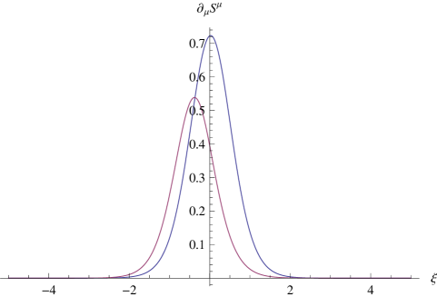
It is easy to check that the solution (45) satisfies (47)-(48). Interestingly, as seen in figure (5), the entropy production is larger on the supersonic side of the wave.

Figure 5: Entropy production as determined by the divergence of the first order entropy current $s^{\mu}=4\pi\eta u^{\mu}$ is plotted versus $\xi=\frac{4u_{\infty}x\pi T}{3}$. For the first order solution (25) (higher curve) the production is symmetric with respect to the front. For the second order solution (45) (lower curve) the entropy production is slightly displaced towards the supersonic side of the jet. The normalization of the vertical axis is such that the difference $\Delta s_{x}$ for the two sides for the first order solution is 1. Notice that the two curves do not have to integrate to the same number, since the asymptotic velocity and temperature differ for the first and second-order solutions, cf. Eqs. (25) and (45).

Similarly we can examine the asymptotic tail of shock waves in the Israel-Stewart theory [56, 57]. This is a theory originally proposed to cure the instantaneous propagation of discontinuities in first order relativistic hydrodynamics. A new tensor $\pi_{\mu\nu}$ is introduced that parametrizes the departure from the ideal fluid:

$${T^{\mu\nu}=p\left(\eta^{\mu\nu}+4u^{\mu}u^{\nu}\right)+\pi^{\mu\nu}\;.}$$

(49)

The tensor $\pi^{\mu\nu}$ is connected to the velocity and temperature fields by

$${\pi^{\mu\nu}+\tau_{\pi}u^{\lambda}\mathcal{D}_{\lambda}\pi^{\mu\nu}=-2\eta\sigma^{\mu\nu}+\tau_{\omega}\left(\omega^{\mu}_{\lambda}\pi^{\lambda\nu}+\omega^{\nu}_{\lambda}\pi^{\mu\lambda}\right)\;,}$$

(50)

where $\mathcal{D}_{\lambda}$ is the so called conformal derivative and $\tau_{\pi}$ (or alternatively $\tau_{\omega}$) is a parameter the value of which has to be determined from microscopics. One often uses the rescaled, dimensionless parameters $\bar{\eta}$ and $\bar{\tau}_{\pi}$ defined by

$${\eta=\bar{\eta}(\pi T)^{3}\;,\quad\tau_{\pi}=\frac{\bar{\tau}_{\pi}}{\pi T}\;.}$$

(51)

For the $\mathcal{N}=4$ superconformal plasma

$${\bar{\eta}=1,\quad\bar{\tau}_{\pi}=\frac{2-\ln 2}{2}\;.}$$

(52)

Alternatively, one may initially leave these parameters undetermined and then choose them to fit specific quantities. In the case of a shock wave $\omega^{\mu\nu}=0$. In order to examine the asymptotic falloff in a linearized theory we perturb the asymptotic values of $u,T$ with (37) and, in addition, one component of the $\pi^{\mu\nu}$ tensor with

$${\pi^{00}(x)=\delta\pi^{00}e^{iqx}\;.}$$

(53)

The resulting three by three system has a solution only if $q$ is given by

$${\frac{iq}{\pi T}=\frac{3v^{2}-1}{v}\frac{\sqrt{1-v^{2}}}{\bar{\eta}+\bar{\tau}_{\pi}\left(1-3v^{2}\right)}\;.}$$

(54)

Notice that there is a pole, which for the $\mathcal{N}=4$ values (52) is located in $v\sim.92$. On the other hand, the fully microscopic calculation based on the gravity dual (and described in section (4)) shows that $q$ remains finite at all $v<1$. This may lead one to choose $\bar{\eta},\bar{\tau}_{\pi}$ in such a way the pole in (54) is located at $v=1$. However, even with this choice the Israel-Stewart theory fails to capture the asymptotic behavior of $q$ at $v\rightarrow 1$. Equation (54) predicts that $q$ increases linearly with $\gamma=\frac{1}{\sqrt{1-v^{2}}}$, whereas the linearized gravity analysis of section (4) predicts $q\propto\gamma^{1/2}$.

2.4 Effective Hydrodynamics

Effective hydrodynamics is the approach where one attempts to model the effect of higher-order terms in the gradient expansion of $T^{\mu\nu}$ with terms that are high in derivatives but linear in velocity. Such an approach has been taken up in Ref. [58] and may seem an ideal way to encode results of a linearized theory. Effective hydrodynamics for a conformal theory in flat space can be summarized by writing the stress tensor as

$${T^{\mu\nu}=p\eta^{\mu\nu}+\left(\rho+p\right)u^{\mu}u^{\nu}+\Pi^{\mu\nu}\;,}$$

(55)

$${\Pi^{\mu\nu}=-2\int dt^{\prime}\int d^{3}x^{\prime}D(x-x^{\prime},t-t^{\prime})\sigma^{\mu\nu}(x^{\prime},t^{\prime})\;,}$$

(56)

$${D(x,t)=\int d\omega d^{3}ke^{-i\omega+ikx}\eta(\omega,k^{2})\;.}$$

(57)

The effective viscosity $\eta(\omega,k^{2})$ is taken to be a function of $\omega,k^{2}$ such that it correctly reproduces the location of the poles of the scalar, shear and sound modes up to the desired order. For the $\mathcal{N}=4$ plasma, it has been calculated up to the fifth order in [58] and found to be

$${\eta=\eta_{0}\left(1+i\eta_{0,1}\omega+\eta_{0,2}\omega^{2}+i\eta_{2,1}\omega k^{2}+i\eta_{0,3}\omega^{3}+\eta_{4,0}k^{4}+\eta_{2,2}\omega^{2}k^{2}+\eta_{0,4}\omega^{4}+\cdots\right)\;,}$$

(58)

$${\eta_{0}=\frac{\rho+p}{2}\;,\quad\eta_{0,1}=2-\ln 2\;,\quad\eta_{2,0}=-\frac{1}{2}\;,}$$

(59)

where we have not given the uncertainties of each coefficient. One can attempt to resum this fifth-order expression into a rational expression with one or two poles [58].

To compute the asymptotic tails of the shock in effective hydrodynamics, we consider again perturbations of the type (37) in the rest frame of the shock. The result is given by

$${\frac{iq}{\pi T}=\frac{3v^{2}-1}{v}\sqrt{1-v^{2}}\frac{\eta_{0}}{\eta(-\frac{vq}{\sqrt{1-v^{2}}},\frac{q^{2}}{1-v^{2}})}\;,}$$

(60)

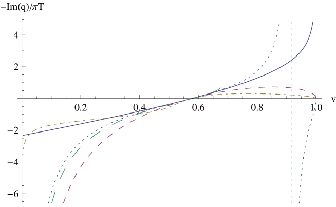
where $v$ is the speed of the fluid relative to the shock. The actual curve $q=q(v)$ is determined by linearized gravity and can only be found numerically; the result is shown in Fig. (6). A simple ansatz for the effective viscosity does not reproduce this curve very well. For example an effective viscosity with one or two poles will always give $q\rightarrow 0$ as $v\rightarrow 1$, in contrast to the behavior following from linearized gravity. On the other hand, as seen in Fig. (6), the expansion of Ref. [58] gives a reasonable approximation for $q$ on the subsonic side of the shock.

We can take the idea of effective hydrodynamics one step further by simply encoding our numerical curve into an expression for $T^{\mu\nu}$, so that agreement with linearized gravity is perfect by construction. In general, any hydrodynamic approximation amounts to reconstructing $T^{\mu\nu}$ from its timelike eigenvector $u^{\mu}$ (cf. Eq. (16)). Consider the fluid at rest with a sound wave of small amplitude $\varepsilon$ propagating along $x$ with momentum $k$ and (in general complex) frequency $\omega(k)$. From conservation of $T^{\mu\nu}$ and the traceless condition we find that the Fourier components of $\delta T^{\mu\nu}$ are given by

$$\delta T^{tt}=\varepsilon,\ \ \delta T^{tx}=\frac{\omega}{k}\varepsilon,\ \ \delta T^{xx}=\frac{\omega^{2}}{k^{2}}\varepsilon,\ \ \delta T^{yy}=\delta T^{zz}=\frac{k^{2}-\omega^{2}}{2k^{2}}\varepsilon\;.$$ (61)

It is now a simple matter to compute the timelike eigenvector of $T^{\mu\nu}$, identify $\delta u=\frac{\omega}{4qT_{0}^{4}}\varepsilon$ as the $x$ component of the four velocity and write $\delta T^{\mu\nu}$ as

$$\delta T^{\mu\nu}=\delta T_{(0)}^{\mu\nu}+\delta T_{(1)}^{\mu\nu}$$ (62)

where $\delta T_{(0)}^{\mu\nu}$ is the variation of the ideal fluid energy momentum tensor $T_{(0)}^{\mu\nu}=(\pi T_{0})^{4}\left(\eta^{\mu\nu}+4u^{\mu}u^{\nu}\right)$ and $\delta T_{(1)}^{\mu\nu}$ is an extra contribution given by

$$\delta T_{(1)}^{xx} = \frac{4}{3k\omega}\left(3\omega^{2}-k^{2}\right)T_{0}^{4}\delta u,$$ (63)

$$\delta T_{(1)}^{yy} = \delta T_{(1)}^{zz}=-\frac{2}{3\omega k}\left(3\omega^{2}-k^{2}\right)T_{0}^{4}\delta u.$$ (64)

In these expressions $\omega$ should be understood as a function of $k$ obtained by solving numerically the gravity equations for the sound wave. Notice that the function $\frac{3\omega^{2}-k^{2}}{\omega k}$ is regular for $k\rightarrow 0$, so $T_{(1)}^{\mu\nu}$ is a well defined function of $\delta u$. It is non-local since it involves an infinite number of derivatives. Nevertheless, in the linear approximation we can work with this energy momentum tensor that reproduces exactly the sound pole and the asymptotic behavior of the shock wave far from the shock. Later, in the numerical section we give an approximate result for the function $\omega(k)$ that could be used, if so desired, to further simplify and approximate $\delta T_{(1)}^{\mu\nu}$. Such effective hydrodynamics is still not sufficient to describe the center of the shock, where the linearized approximation is not applicable, but at least it summarizes all the information we were able to extract from gravity without attempting to find the full numerical solution to the Einstein equations in the bulk.

Figure 6: The solid (blue) line represents the numerical results discussed in section (4). The (purple) dashed line is the first order hydrodynamics result and the (green) dashed line is the second order result. The (blue) dotted line is the Israel-Stewart result and the dotted-dashed line is the result for the effective hydrodynamics theory of section (2.4). None of the theories captures the $v\rightarrow 1$ asymptotics of the numerical result.

3 Shock waves in the gravity-hydrodynamics correspondence

In a strong shock wave, the region near the shock is beyond the hydrodynamic approximation and can only be described as a jump in the hydrodynamic quantities. In the case of the strongly coupled ${\cal N}=4$ plasma, hydrodynamics ceases to be valid at distances shorter than the inverse temperature. However, at those distances the bulk description in terms of gravity does not break down suggesting that gravity can resolve the shock waves and provide a smooth description for them. However the velocity and temperature are not well defined in the region of the shock, so the best characterization is in terms of the energy density, namely $T^{tt}(x)$. In this section we first study such function in the case of weak or hydrodynamic shocks. In that case we can reproduce the results of the previous section and obtain the dual metric (within the hydrodynamic approximation). Afterwards we consider strong shocks and, by using linearized gravity, obtain the width of the shock, as determined by the exponential tails on both sides. This is detailed information that can only be obtained from a microscopic theory of the system. In principle, one would like to go further and obtain $T^{tt}(x)$ by solving the Einstein equations in the bulk numerically, but such a calculation is beyond the scope of this paper.

3.1 Weak shocks: an explicit solution in the fluid-gravity correspondence

The four conservation equations $\partial_{\mu}T^{\mu\nu}=0$ are not enough to determine the nine independent components of $T^{\mu\nu}$ in the boundary theory. Hydrodynamics amounts to a restriction on $T^{\mu\nu}$ by providing an expression for it in terms of four variables, the velocity $v_{i=1,2,3}$ and temperature $T$, which are then determined from the conservation equations. The expression for $T^{\mu\nu}$ is given as a derivative expansion, and its precise form can only be determined from a microscopic theory of the system.

From the dual gravitational point of view, the energy momentum tensor sets the boundary conditions for an asymptotically AdS metric and the conservation equations $\partial_{\mu}T^{\mu\nu}=0$ are necessary consistency conditions for the existence of a solution to the Einstein equations with such boundary data. As recently explained by Bhattacharyya et al. [50] those metrics generically have naked singularities. The condition of the metric being non-singular imposes a restriction to $T^{\mu\nu}$, which is a counterpart of the restriction seen in the hydrodynamic construction. In fact, when this analysis is done in a derivative expansion, as shown in [50], it provides a microscopic derivation of the hydrodynamic equations for the strongly coupled ${\cal N}=4$ plasma.

In this section we use the BHMR construction [50] to obtain the metric dual to the shock waves in the hydrodynamic regime up to terms which are third order in the derivative expansion.

Let us start by summarizing the procedure as adapted to our particular problem. The starting point is the boosted black brane in Eddington-Filkenstein coordinates:

$$ds_{(0)}^{2}=-2u_{\mu}dx^{\mu}dr+\frac{\left(\pi T(x)\right)^{4}}{r^{2}}u_{\mu}u_{\nu}dx^{\mu}dx^{\nu}+r^{2}\eta_{\mu\nu}dx^{\mu}dx^{\nu}\;,$$ (65)

where

$$u^{\mu}=(u^{0}(x),u(x),0,0),\ \ \ \ \ u^{0}(x)=\sqrt{1+u(x)^{2}}\;.$$ (66)

Since $u(x)$ and $T(x)$ are not constant this metric does not solve the Einstein equations

$$\bar{G}_{MN}=R_{MN}+4g_{MN}=0\;,$$ (67)

where $M,N=r,t,x,y,z$ denote 5-dimensional indices (whereas $\mu,\nu=t,x,y,z$ denote four-dimensional indices). To find a solution we introduce a formal parameter $\epsilon$ and expand

$$u^{\mu} = u_{\mu}^{(0)}+\epsilon u_{\mu}^{(1)}+\epsilon^{2}u_{\mu}^{(2)}+\epsilon^{3}u_{\mu}^{(3)}+{\cal O}(\epsilon^{4})\;,$$ (68)

$$T(x) = T_{(0)}(x)+\epsilon T_{(1)}(x)+\epsilon^{2}T_{(2)}(x)+\epsilon^{3}T_{(3)}(x)+{\cal O}(\epsilon^{4})\;.$$ (69)

At the same time, the metric is corrected by adding an expansion

$$ds^{2}=ds_{(0)}^{2}+\epsilon ds_{(1)}^{2}+\epsilon^{2}ds_{(2)}^{2}+{\cal O}(\epsilon^{3})\;.$$ (70)

The tensor $\bar{G}_{MN}$ is expanded in powers of $\epsilon$ with the rule that each $x$-derivative counts as one extra power of $\epsilon$. The equations are solved order by order. For that purpose it is convenient to introduce the vector

$$\tilde{u}^{\mu}=(u(x),u^{0}(x),0,0)\;,$$ (71)

orthogonal to $u^{\mu}$. In this way the metric corrections can be parametrized as

$$ds^{2}_{(n)} = (s_{1}^{(n)}+s_{2}^{(n)})u_{\mu}u_{\nu}dx^{\mu}dx^{\nu}+s_{2}^{(n)}\eta_{\mu\nu}dx^{\mu}dx^{\nu}+2s_{3}^{(n)}u_{\mu}dx^{\mu}dr+s_{V}^{(n)}\tilde{u}_{\mu}u_{\nu}dx^{\mu}dx^{\nu}$$ (72)

$$+s_{T}^{(n)}\left(\tilde{u}_{\mu}\tilde{u}_{\nu}dx^{\mu}dx^{\nu}-\frac{1}{2}(dy^{2}+dz^{2})\right)\;,$$

where the functions $s_{1,2,3}^{(n)},s_{V},s_{T}$ describe scalar, vector and tensor perturbations classified according to the local $SO(3)$ group that leaves $u^{\mu}$ invariant. Notice that each $ds^{2}_{(n)}$ should in turn be expanded using (68). Following [50] we make the gauge choice $g^{(n)}_{rr}=0$, $g^{(n)}_{\mu r}\sim u_{\mu}$ and $g_{(0)}^{\mu\nu}g^{(n)}_{\nu\mu}=0$ for all $n>0$. In that case it is convenient to parametrize the fluctuations as

$$s_{1}^{(n)}= \frac{1}{r^{2}}k^{(n)}(x,r),\ s_{2}^{(n)}=r^{2}h^{(n)}(x,r),\ s_{3}^{(n)}=\frac{3}{2}h^{(n)}(x,r),$$ (73)

$$\ s_{V}=\frac{1}{r^{2}}j^{(n)}(x,r),\ s_{T}^{(n)}=r^{2}\alpha^{(n)}(x,r)\;,$$ (74)

In order to solve the equations order by order it is convenient to decompose $\bar{G}_{MN}$ into its scalar, vector and tensor parts which decouples the equations. The procedure is in principle straightforward, and we proceed to describe the results.

Order 1.

The first equations that we obtain are $u_{0}^{\prime}=0$, $T_{(0)}^{\prime}=0$ implying that

$$u_{(0)}(x)=u_{(0)},\ \ \ T_{(0)}(x)=T_{(0)}\;,$$ (75)

namely they are constant functions. In that case the zero order metric is an exact solution and there is no first order correction to the metric:

$$h^{(1)}=k^{(1)}=j^{(1)}=\alpha^{(1)}=0\;.$$ (76)

The temperature however is corrected to

$$T^{(1)}=-\frac{\sqrt{2}}{3}T_{(0)}u_{(1)}\;.$$ (77)

Order 2.

The first equation we find is

$$u_{(1)}^{\prime}(2u_{(0)}^{2}-1)=0\;.$$ (78)

We can take $u_{(1)}$ constant which leads us to a trivial solution, or otherwise we require $u_{(0)}=\frac{1}{\sqrt{2}}$ implying that the zero order solution describes a fluid moving at the speed of sound, which is the appropriate starting point to describe shocks in the hydrodynamic approximation. The other equations give:

$$h^{(2)}=0,\ \ k^{(2)}=\frac{2}{3}r^{3}u_{(1)}^{\prime},\ \ j^{(2)}=-\frac{2}{\sqrt{3}}r^{3}u_{(1)}^{\prime},\ \ \alpha^{(2)}=\frac{u_{(1)}^{\prime}}{3\pi T_{(0)}}F_{1}\left(\frac{r}{\pi T_{(0)}}\right)\;,$$ (79)

where

$$F_{1}(y)=\ln\left(\frac{(1+y^{2})(1+y)^{2}}{y^{4}}\right)-2\arctan y+\pi\;.$$ (80)

Notice that at this order $u_{(1)}$ is undetermined. This is a particular property of our solution that requires us to go to higher orders to obtain the metric.

Order 3.

The first equation we obtain is

$$u_{(1)}^{\prime\prime}=\frac{8}{3}\pi T_{(0)}u_{(1)}u_{(1)}^{\prime}\;,$$ (81)

which allows us to solve for $u_{(1)}$ as we do further below. The components of the metric are corrected by

$${h^{(3)}}$$

(82)

with

$$F_{2}(y) = \frac{1}{2}(y^{4}-1)\left(2\arctan y+\ln\left(\frac{1+y^{2}}{(1+y)^{2}}\right)\right)-\frac{1}{2}\pi y^{4}+y^{3}+y^{2}-\frac{25}{12}\;,$$ (83)

$$F^{\prime}_{3}(y) = \frac{1}{y^{5}-y}\left\{2(1-y^{3})\left(\arctan y-\frac{\pi}{2}-\ln(1+y)\right)+(1+y^{3})\ln(1+y^{2})\right.$$ (84)

$$\left.-4y^{3}\ln y+7-2\ln 2-\frac{2(1+y)}{1+y^{2}}-\frac{2}{1+y}-4y^{2}\right\}\;.$$

We give the derivative of $F_{3}$ since it is the function that enters in subsequent calculations. It can be integrated explicitly in terms of dilogarithms but the expression is not very illuminating. The temperature is given by

$$\pi T_{(2)}=-\frac{\sqrt{2}}{3}\pi T_{(0)}u_{(2)}+\frac{1}{3}u_{(1)}^{\prime}\;.$$ (85)

We want to write the metric up to order $\epsilon^{2}$ which requires computing $u_{(2)}$. Since it is undetermined at this order we continue the expansion.

Order 4.

At this order we only look for the equation determining $u_{(2)}$. However we need to include and keep track of the terms $u_{(3)}$, $T_{(3)}$ , $h_{(4)}$ etc. to be sure that they do not appear in such equation. What we get is

$$u_{(2)}^{\prime\prime}-\frac{8}{3}\pi T_{(0)}(u_{(1)}u_{(2)})^{\prime}=\frac{\sqrt{2}}{3}(7-2\ln 2)u_{(1)}^{\prime}{}^{2}-\frac{4\sqrt{2}}{9}\pi T_{(0)}u_{(1)}^{2}u_{(1)}^{\prime}(1+4\ln 2)\;.$$ (86)

The last equation, together with (81), can be easily solved to obtain, at this order

$$u = u_{(0)}+u_{(1)}+u_{(2)}\;,$$ (87)

$$u_{(0)} = \frac{1}{\sqrt{2}}\;,$$ (88)

$$u_{(1)} = -u_{\infty}\tanh\xi\;,$$ (89)

$$u_{(2)} = \frac{u_{\infty}^{2}}{6}\left[4\sqrt{2}(1-\ln 2)\frac{\ln\cosh\xi}{\cosh^{2}\xi}+5\sqrt{2}\left(\tanh^{2}\xi+\tanh\xi+\frac{\xi}{\cosh^{2}\xi}\right)\right]\;,$$ (90)

where

$$\xi=\frac{4\pi T_{(0)}u_{\infty}}{3}\,x\;,$$ (91)

and we set the formal parameter $\epsilon=1$. It is interesting to note that the equation for $u_{(1)}$ determines that the fluid reaches the shock wave supersonically and leaves subsonically. In other words, we are not free to exchange the subsonic and supersonic sides of the shock. The reason is that are choosing gravity solutions which are regular in the infalling Eddington-Filkenstein coordinates as appropriate for a black hole. The constant $u_{\infty}$ is arbitrary and determines the amplitude of the shock, namely, the asymptotic value of the velocity. For consistency of the approximation we require $u_{\infty}\ll\frac{1}{\sqrt{2}}$. In fact, $u_{\infty}$ plays the role of the small parameter, as can be seen from the fact that the velocity depends on $x$ through $\xi$ and so each $x$ derivative brings in an extra power of $u_{\infty}$. The behavior at infinity is given by

$$u(x\rightarrow\pm\infty) \simeq \frac{1}{\sqrt{2}}\mp u_{\infty}\pm 2u_{\infty}e^{\mp 2\xi}\left(1+\frac{1}{3}u_{\infty}(4\sqrt{2}-4\ln 2\pm 5\sqrt{2})\xi\right)$$ (92)

$$\simeq \frac{1}{\sqrt{2}}\mp u_{\infty}\pm 2u_{\infty}e^{\mp 2\xi+\frac{1}{3}u_{\infty}(4\sqrt{2}-4\ln 2\pm 5\sqrt{2})\xi}\;.$$ (93)

We write the correction in the exponential form for an easier comparison with the hydrodynamic result. For the temperature we have

$$T(x\rightarrow\pm\infty)=T_{(0)}\pm\frac{\sqrt{2}}{3}T_{(0)}u_{\infty}\;.$$ (94)

For the velocity we have

$$v(x\rightarrow\infty) \simeq \frac{1}{\sqrt{3}}+\delta v_{+}=\frac{1}{\sqrt{3}}-\frac{2\sqrt{2}}{3\sqrt{3}}u_{\infty}+\frac{14}{9\sqrt{3}}u_{\infty}^{2}\;,$$ (95)

$$v(x\rightarrow-\infty) \simeq \frac{1}{\sqrt{3}}+\delta v_{-}=\frac{1}{\sqrt{3}}+\frac{2\sqrt{2}}{3\sqrt{3}}u_{\infty}-\frac{2}{3\sqrt{3}}u_{\infty}^{2}\;.$$ (96)

The first check is that the condition (6)

$$v(-\infty)v(+\infty)=\frac{1}{3}+{\cal O}(u_{\infty}^{3})\;,$$ (97)

is satisfied to the considered order. From eq. (93), the exponential tail is given by

$$v(x\rightarrow\pm\infty)=\frac{1}{\sqrt{3}}+\delta v_{\pm}+c_{\pm}e^{iq_{\pm}x}\;,$$ (98)

for some constants $c_{\pm}$ and the penetration depth determined by

$$\frac{iq_{\pm}}{\pi T_{\pm}}=2\sqrt{6}\delta v_{\pm}+6\sqrt{2}\delta v_{\pm}^{2}(1-\ln 2)\;,$$ (99)

in complete agreement with the hydrodynamic calculation. This is not surprising since the hydrodynamic equations arise from gravity. The calculation in this section, however, allows us to compute in addition the dual metric, which to this order is given by

$$ds^{2} = -2u_{\mu}dx^{\mu}dr+\frac{1}{r^{2}}((\pi T)^{4}+k)u_{\mu}u_{\nu}dx^{\mu}dx^{\nu}+r^{2}\eta_{\mu\nu}dx^{\mu}dx^{\nu}+\frac{1}{r^{2}}j\tilde{u}_{\mu}u_{\nu}dx^{\mu}dx^{\nu}$$ (101)

$$+\alpha r^{2}(\tilde{u}_{\mu}\tilde{u}_{\nu}dx^{\mu}dx^{\nu}-\frac{1}{2}(dy^{2}+dz^{2}))\;,$$

where $u^{\mu}=(\sqrt{1+u^{2}},u,0,0)$, $\tilde{u}^{\mu}=(u,\sqrt{1+u^{2}},0,0)$ and $u$ should be expanded as $u=u_{(0)}+u_{(1)}+u_{(2)}$ using the $u_{(n)}$ computed in (90). The temperature is also expanded as

$$T=T_{(0)}-\frac{\sqrt{2}}{3}T_{(0)}u_{(1)}-\frac{\sqrt{2}}{3}T_{(0)}u_{(2)}+\frac{1}{3\pi}u_{(1)}^{\prime}\;,$$ (102)

whereas the other functions entering the metric are given by

$$k = \frac{2}{3}r^{3}(u_{(1)}^{\prime}+u_{(2)}^{\prime})-\frac{\sqrt{2}}{3}r^{2}u_{(1)}^{\prime\prime}\;,$$ (103)

$$j = -\frac{2}{\sqrt{3}}\,r^{3}(u_{(1)}^{\prime}+u_{(2)}^{\prime})+\frac{4\sqrt{2}}{3\sqrt{3}}u_{(1)}u_{(1)}^{\prime}(\pi T_{(0)})^{3}F_{2}\!\left(\frac{r}{\pi T_{(0)}}\right),$$ (104)

$$\alpha = \frac{u_{(1)}^{\prime}+u_{(2)}^{\prime}}{3\pi T_{(0)}}F_{1}\!\left(\frac{r}{\pi T_{(0)}}\right)-\frac{4\sqrt{2}}{9\pi T_{(0)}}u_{(1)}u_{(1)}^{\prime}F_{3}\!\left(\frac{r}{\pi T_{(0)}}\right)\;,$$ (105)

with the $F_{1,2,3}$ as defined above. The expansion parameter is the strength of the shock as determined by the constant $u_{\infty}$ appearing in $u_{(n)}$.

4 Strong shocks: the linearized gravity approximation

Strong shocks are characterized by large gradients of velocity and temperature and cannot be studied within hydrodynamics: we can say that hydrodynamics does not resolve their profiles. However, the gauge-gravity correspondence is not limited to small gradients, and so the gravity side of it should contain information about strong shocks as well. We now discuss how that information can be extracted.

In principle, we expect that there are exact solutions to the 5-dimensional Einstein equations, and those solutions describe strong shocks exactly. This belief is based on the observation that the asymptotic values of $u_{\mu}$ and $T$ on the far left and far right of the shock have vanishing gradients and are therefore well reproduced even by the ideal hydro (see Sec. 2). On the gravity side, to each of these asymptotics, there corresponds a 5-dimensional AdS black brane, suitably boosted and with a suitable value of the temperature. Then, there must be a 5d solution describing a stationary wave that smoothly interpolates between these two regions—the gravity dual of a strong shock.

The exact solution (assuming it exists) described in the preceding paragraph would tell us all there is to know about a strong shock, in particular, the profile of the average energy density, $\epsilon(x)$. So far, however, we have not been able to find any such solution explicitly. In this section, we provide partial information about the profile of a strong shock, obtained by looking at linearized gravity on the backgrounds corresponding to each of the two asymptotic regions ($x\to\pm\infty$).

4.1 Equations of linearized gravity

In linearized gravity, one writes the metric in the form $g_{\mu\nu}=g^{(0)}_{\mu\nu}+h_{\mu\nu}$, where $g^{(0)}_{\mu\nu}$ is the metric of the AdS black brane, and $h_{\mu\nu}$ is a perturbation, and works to the first order in the perturbation. Solutions to the linearized Einstein equations are known as quasinormal modes. In this paper, we consider solutions that depend only on the coordinate ($x$) along the direction in which the shock propagates and, possibly, time. In this section we adopt the convention $\pi T=1$, the temperature dependence can be recovered by multiplying the modes by $\pi T$. Due to the translational invariance along the brane directions, we can search for these solutions in the form

$$h_{\mu\nu}(t,x,r)=r^{2}H_{\mu\nu}(r)e^{-i\omega t+iqx}\,.$$

We adopt the convention that $\omega$ and $q$ refer to the boosted frame, moving at the speed of the shock, and their primed counterparts, $\omega^{\prime}$ and $q^{\prime}$, to the unboosted frame, connected with the fluid. Note that there are actually two such unboosted frames (the fluid on the two sides of the shock moves with different velocities), but in the linearized approximation the two sides are disconnected and can be considered separately.

Linearized gravity has by now become a familiar tool in studies of the kinetics of the strongly coupled ${\cal N}=4$ plasma but in a setting that is typically different from ours. In many cases (as, for example, in the computation of the viscosity [51]) one considers relaxation of an initial perturbation. Then, one picks a real wavenumber $q$ and looks for the corresponding (complex) frequencies. Here, in contrast, we are interested in propagation of a boundary disturbance, that is, in how far a perturbation with a given frequency extends into the plasma on either side of the shock. For this, we pick a real $\omega$ and look for the corresponding (complex) $q$. Specifically, we will be interested in perturbations with $\omega=0$, as we expect these to describe the behavior of the average energy density of a shock wave sufficiently far away from it.

A classification of the quasinormal modes of an (unboosted) AdS black brane has been given in [59]; a comprehensive recent review of quasinormal modes is [60] . According to that classification, metric fluctuations group into several channels, corresponding to different gauge-invariant combinations of the components of $H_{\mu\nu}$. Here, we are interested in the sound channel. The corresponding quasinormal modes satisfy the equation [59]

$$Z^{\prime\prime}+P(u)Z^{\prime}+Q(u)Z=0\,,$$ (106)

where primes denote derivatives with respect to $u=r_{0}^{2}/r^{2}$,

$$P(u) = -\frac{3{\omega^{\prime}}^{2}(1+u^{2})+{q^{\prime}}^{2}(2u^{2}-3u^{4}-3)}{uf(u)[3{\omega^{\prime}}^{2}+{q^{\prime}}^{2}(u^{2}-3)]}\,,$$

$$Q(u) = -\frac{4{q^{\prime}}^{2}u^{2}}{f(u)[3{\omega^{\prime}}^{2}+{q^{\prime}}^{2}(u^{2}-3)]}+\frac{3{\omega^{\prime}}^{4}+{q^{\prime}}^{4}(u^{4}-4u^{2}+3)+{\omega^{\prime}}^{2}{q^{\prime}}^{2}(4u^{2}-6)}{4uf^{2}(u)[3{\omega^{\prime}}^{2}+{q^{\prime}}^{2}(u^{2}-3)]}\,,$$

and $f(u)=1-u^{2}$. Remember that in these expressions, $\omega^{\prime}$ and $q^{\prime}$ are in units of $\pi T$ and refer to the unboosted frame. They are related to the frequency and wavenumber in the boosted frame by the Lorentz transformation

$$\omega^{\prime} = \omega\cosh\beta-q\sinh\beta\,,$$ (107)

$$q^{\prime} = -\omega\sinh\beta+q\cosh\beta\,,$$ (108)

where $\tanh\beta=v$, the speed of the shock. For static perturbations, we set $\omega=0$ and substitute the resulting expressions for $\omega^{\prime}$ and $q^{\prime}$ into Eq. (106), to obtain:

$$P(u) = \frac{3+3u^{2}-5\gamma^{2}u^{2}+3\gamma^{2}u^{4}}{uf(u)(\gamma^{2}u^{2}-3)}\,,$$ (109)

$$Q(u) = -\frac{4\gamma^{2}u^{2}}{f(u)(\gamma^{2}u^{2}-3)}+q^{2}\frac{\gamma^{2}u^{2}-1}{4uf^{2}(u)}\,,$$ (110)

where we have used the shorthand $\gamma=\cosh\beta$.

The same expressions can be obtained by starting directly in the boosted frame. In this case, the unperturbed metric is

$$ds^{2}_{0}=r^{2}\eta_{\mu\nu}dx^{\mu}dx^{\nu}+\frac{r_{0}^{4}}{r^{2}}(dt\cosh\beta-dx\sinh\beta)^{2}+\frac{dr^{2}}{r^{2}(1-r_{0}^{4}/r^{4})}\,,$$

and the perturbation reads

$$ds^{2}_{1}=r^{2}\left[H_{00}dt^{2}+H_{11}dx^{2}+2H_{01}dtdx+H(dy^{2}+dz^{2})\right]e^{iqx}$$

(all $H_{\mu\nu}$ are functions of $r$ only). The relevant gauge-invariant combination (at $\omega=0$) is

$${Z(r)=H_{00}(r)+\left(1+\frac{r_{0}^{2}}{r^{4}}\gamma^{2}\right)H(r)\;,}$$

(111)

and satisfies Eq. (106) with the coefficient functions given by Eqs. (109) and (110).

For computation of properties of the plasma via the gauge-gravity correspondence, we only need to consider Eq. (106) in the region outside the horizon, $r_{0}<r<\infty$, which we will refer to as the physical region. In terms of the variable $u$, it corresponds to $0<u<1$. A noteworthy property of the coefficient functions (109) and (110) is that, at sufficiently large boost velocities,

$$\cosh\beta>\cosh\beta_{\rm cr}=\sqrt{3}\,,$$ (112)

$P$ and $Q$ both have poles inside the physical region, at

$${u=u_{1}\equiv\frac{\sqrt{3}}{\cosh\beta}\,.}$$

(113)

From the outset, we might have anticipated that we would need to impose boundary conditions at the boundaries of the physical region, $u\to 0$ and $u\to 1$, but not at any interior point. We therefore need to explore the nature of the singularity at $u=u_{1}$ in more detail.

Let us search for solutions near $u=u_{1}$ in the form $Z\sim(u-u_{1})^{s}$. For the exponent $s$, we find two roots,

$${s=0\mbox{ or }3.}$$

(114)

Fuchs’s theorem [61] guarantees that the larger root correspond to a regular solution, expandable in powers of $w=u-u_{1}$ as follows: $Z=w^{3}+O(w^{4})$. As for the solution corresponding to the smaller root, in general, we expect it to have the form

$$Z(u)=c_{0}+c_{1}w+c_{2}w^{2}+c_{3}w^{3}+c_{3}^{\prime}w^{3}\ln w+\ldots$$ (115)

The recursion equation for the coefficients $c_{n}$, which is obtained by substituting Eq. (115) in Eq. (106), degenerates at the order (and only at the order) at which the second solution appears, in our case the order $w^{3}$. Whether or nor the logarithmic term in (115) is nonzero then depends on the precise values of the coefficients of all the terms up to $O(w)$ order in the expansions of $P(u)$ and $Q(u)$. As it turns out, there is a curious cancellation among these terms, such that $c_{3}^{\prime}=0$ for all values of $\gamma$ and $q$. We conclude that both solutions are regular at $u=u_{1}$, and a boundary condition there is not required.

4.2 Boundary conditions. Irreversibility

The choice of boundary conditions for quasinormal modes that is suitable for applications of the gauge-gravity duality to kinetic theory has been discussed in the literature (see, for example, Ref. [51]), and we do not deviate from it here. Our computation, however, requires an analytical continuation of these boundary conditions, which is the subject of this subsection.

At $u\to 0$ (the boundary of the AdS space) we use the standard

$${Z(0)=0\,.}$$

(116)

At $u\to 1$ (the near-horizon region), we first consider real $\omega^{\prime}$ and pick, as usual, the wave infalling with respect to the black brane:

$${Z(u\to 1)\sim(1-u)^{-i\omega^{\prime}/4}\,.}$$

(117)

For the present problem, having to do with propagation of a perturbation in space, rather than in time, we need to analytically continue this expression to complex $\omega^{\prime}$ given by the Lorentz transformation (107) ($\omega^{\prime}$ is complex because so is $q$). In particular, for the static case ($\omega=0$), we have $\omega^{\prime}=-q\sinh\beta$ and thus

$${Z(u\to 1)\sim(1-u)^{\frac{1}{4}iq\sinh\beta}\,.}$$

(118)

This choice is equivalent to choosing the solution that is regular in infalling Eddington-Filkenstein coordinates as done in section 3.1. There is an exceptional case $\beta=\beta_{\rm cr}$, the critical value given by Eq. (112). For this value of $\beta$, the analytical continuation to $\omega=0$ causes confluence of the singularities at $u=1$ and $u=u_{1}$, which modifies the asymptotic behavior near $u=1$. We consider this case separately later in this subsection.

Recall that $Z(u)$ corresponds, via the gauge-gravity duality, to a perturbation in the plasma that depends on $x$ as $\exp(iqx)$. On physical grounds, we expect that perturbations corresponding to the tails of a shock at $x\to\pm\infty$ decay away from the shock. This means that we must pick $q$ with a positive (negative) $\mbox{Im}~{}q$ for the fluid at positive (negative) $x$. Recall also that positive (negative) $x$ correspond to the subsonic (supersonic) side of the shock. Thus, according to Eq. (118), $Z(u)$ is regular at the horizon on the supersonic side but singular on the subsonic one.

Formulating a boundary problem for the regular case presents no difficulty: the second solution to Eq. (106) diverges at $u\to 1$, and the boundary condition (118) selects the one that does not. The singular case (${\rm Im}q>0$) is a bit trickier: we wish to retain the divergent solution and reject the convergent one. To achieve that, we peel off the singular part, as follows:

$${Z(u)=(1-u)^{s}\Psi(u)\,,}$$

(119)

where

$${s=-\frac{1}{4}i\omega^{\prime}=\frac{1}{4}iq\sinh\beta}$$

(120)

(${\rm Re}s<0$), and demand that $\Psi(u)$ is analytic at $u=1$. This works whenever

$${2s\neq\mbox{integer}\;.}$$

(121)

Indeed, the regular solution behaves as $(1-u)^{-s}$, and the corresponding $\Psi$ as $(1-u)^{-2s}$. Provided the inequality (121) is satisfied, this is not analytic and is rejected by our boundary condition.

Note that the inequality (121) is sufficient but not necessary for the singular boundary problem to make sense. Suppose (121) is not satisfied for some values of $q$ and $\beta$, but both solutions for $\Psi$ are regular at $u=1$. We consider such a $q$ to be an eigenvalue of our problem (at that particular $\beta$), because we can always form a linear combination of the two regular solutions that satisfies the second boundary condition (116). On the other hand, it is a priori possible that (121) fails in such a way that one of the solutions for $Z$ contains a logarithm of $1-u$. In this case, we truly have no recourse; indeed, the singular part cannot even be peeled off as in (119). Interestingly, the condition (121) never breaks down for the “main” branch of $q(v)$, as defined below.

We anticipate that there is more than one eigenvalue of $q$ for each value of the shock’s speed $v$. We refer to these as different branches and denote them as $q_{n}(v)$. Let us mention some of the properties of these eigenvalues for the case $\omega=0$.

First, setting $q=-i\kappa$ makes all the coefficients in the equation (106) real and turns the condition (118) real as well. We conclude that the eigenvalues $q_{n}(v)$ are all purely imaginary, and $s$ all purely real. (This is not the case at $\omega\neq 0$.)

Second, while the functions (109) and (110) do not depend on the sign of $q$, the condition (118) does. Hence, the set of the eigenvalues $q_{n}(v)$ at a nonzero $v$ is not symmetric about $q=0$. The reflection $q\to-q$, without changing the direction of the shock’s velocity, is equivalent to reflection of both space and time: $x\to-x$ and $t\to-t$. In particular, it exchanges the subsonic and supersonic sides of the shock. The absence of symmetry under $q\to-q$ corresponds to the condition (already noted in Sec.(2.2)) that the fluid must be supersonic in front of the shock and subsonic behind it, and never vice versa—a condition that reflects, ultimately, the second law of thermodynamics. In calculations on the gravity side, the source of this irreversibility is the choice of the infalling wave in Eq. (117).

The main branch. The branch $q_{0}(v)$, for which $\exp(iqx)$ decays away from the shock the slowest, will be referred to as the “main” branch and often denoted simply as $q(v)$. This is the branch that crosses zero at $v=1/\sqrt{3}$ and is the only one seen in the small-gradient (hydrodynamic) approximation discussed in Sec. 2.

The exceptional case. The preceding discussion of the boundary conditions does not apply to the exceptional case $\omega=0$, $\beta=\beta_{\rm cr}$, when the singularities at $u=1$ and $u=u_{1}$ coincide. This case needs to be considered separately. At $\omega=0$ and $\beta=\beta_{\rm cr}$, Eq. (106) becomes

$${Z^{\prime\prime}+\frac{3u^{2}-1}{uf(u)}Z^{\prime}+\frac{1}{f^{2}(u)}\left(4u^{2}+q^{2}\frac{3u^{2}-1}{4u}\right)Z=0\,.}$$

(122)

Solutions near $u=1$ are of the form $Z(u)\sim(1-u)^{s}$ with

$${s=1\pm i\frac{q}{2\sqrt{2}}\,.}$$

(123)

Consider the substitution

$${Z(u)=(1-u^{2})^{1/2}\Phi(u)\,.}$$

(124)

Eq. (122) becomes

$${\Phi^{\prime\prime}-\frac{1}{u}\Phi^{\prime}+\frac{4u^{3}+q^{2}(3u^{2}-1)}{4uf^{2}(u)}\Phi=0\,.}$$

(125)

Note that for $q^{2}=-2$ the coefficients in Eq. (122) are all regular at $u=1$. Hence, $q=\pm i\sqrt{2}$ are eigenvalues of the boundary problem. Since $\beta=\beta_{\rm cr}$ is supersonic, only

$${q=-i\sqrt{2}}$$

(126)

is physical; it lies on the main branch. Curiously, although the behavior at $u=1$ prescribed by Eq. (123) is in general different from that prescribed by Eq. (118), for $q=-i\sqrt{2}$ (and $s=1/2$) they coincide. As a result, the curve $q(v)$ corresponding to the main branch is continuous at $v=v_{\rm cr}$.

For branches above the main branch, $iq_{n}(v_{\rm cr})$ is large, so that only one of the solutions to Eq. (122) is regular at $u=1$. The boundary condition is to choose the regular solution, which corresponds to choosing the plus sign in Eq. (123). This is equivalent to using

$${Z(u)=(1-u)^{iq/2\sqrt{2}}\Psi(u)}$$

(127)

[cf. Eq. (118)] but allowing $\Psi(u)$ to vanish (linearly) at $u=1$. Indeed, as $v$ goes through $v_{\rm cr}$, $\Psi(1)$ goes continuously through zero. Thus, these other branches are also continuous at $v=v_{\rm cr}$.

4.3 Quasinormal modes for special values of $v$

4.3.1 $v=0$ (fluid at rest)

The case of a plasma at rest has already been studied. In particular, as argued for example in [62], the eigenvalue $q$ is given by the lowest glueball mass in Witten’s $QCD_{3}$ construction [63]. The reason is that, in the Euclidean space, both finite temperature $\mathcal{N}=4$ and $QCD_{3}$ are dual to the same $AdS$ black hole. For the channel we are considering, the glueball mass was computed in [64] giving $iq=2.3361$ in perfect agreement with our numerical results. This provides a nice check of the calculation although we should point out that, in the frame where the shock wave is at rest, the velocity of the fluid is always $v>\frac{1}{3}$ so $v=0$ is not directly relevant to our problem.

4.3.2 $v=1/\sqrt{3}$ (the speed of sound)

This is the limit when the strength of the shock (as measured by changes in various quantities between the left and right of the shock) vanishes. As we have seen in section (2), in this limit $q=0$. The corresponding solution to Eq. (106) is

$$Z(u)=u^{2}\,.$$

4.3.3 $v=\sqrt{2/3}$ (the singular point)

In this case the pole corresponding to the horizon $u=1$ merges with the one at $u=u_{1}$ since $v=\sqrt{2/3}$ implies $u=u_{1}$. Interestingly in this case we can find the exact eigenvalue $iq=\sqrt{2}$ and the eigenfunction is given in terms of a hypergeometric function:

$$y(u)=u\sqrt{1-u^{2}}\left(\frac{1+u}{u}\right)^{\frac{1+i}{2}}F_{2,1}\left(\frac{3+i}{2},\frac{-1+i}{2};1+i;1+\frac{1}{u}\right)\;.$$ (128)

With this definition we find

$$Z(u)=-\mbox{Re}(y(u))+C_{1}\mbox{Im}(y(u))\;,$$ (129)

where $C_{1}$ is a constant that we evaluate numerically to be $C_{1}=0.38898$ from the boundary conditions.

4.3.4 $v\rightarrow 1$ (ultrarelativistic limit)

Numerical solution (described in the next subsection) shows that the values of $s$, Eq. (120), for the physical branches become large in the limit $v\to 1$, and the maxima of the eigenfunctions scale towards $u=0$. This suggests that we can obtain an equation applicable in the ultrarelativistic limit by neglecting $u$ in comparison with unity in the coefficient functions (109) and (110). We obtain

$${P(u)=\frac{3-5\gamma^{2}u^{2}}{u(\gamma^{2}u^{2}-3)}\;,}$$

(130)

$${Q(u)=-\frac{4\gamma^{2}u^{2}}{\gamma^{2}u^{2}-3}+q^{2}\frac{\gamma^{2}u^{2}-1}{4u}\;.}$$

(131)

These expressions suggest further that we define a new variable $x$, as follows:

$$x=\frac{u^{2}}{u_{1}^{2}}=\frac{1}{3}u^{2}\cosh^{2}\beta\,,$$ (132)

and take the formal limit $\cosh\beta\to\infty$ while keeping $x$ fixed. Eq. (106) becomes

$$Z^{\prime\prime}+\frac{2}{1-x}Z^{\prime}+\frac{p^{2}}{16}\left(3-\frac{1}{x}\right)\frac{1}{\sqrt{x}}Z=0\,,$$ (133)

where primes now denote derivatives with respect to $x$, and

$$p^{2}\equiv q^{2}u_{1}=\frac{q^{2}\sqrt{3}}{\cosh\beta}\,.$$ (134)

The change of variables (132) and the limit $\cosh\beta\to\infty$ map the physical region $0<u<1$ to $0<x<\infty$, with the Dirichlet boundary conditions at both ends. As before, the point $x=1$ (formerly $u=u_{1}$) is a singular point of the equation but not of either of the two linearly independent solutions. Thus, in numerical integrations we can circumvent this point by first displacing it into the complex plane, i.e., replacing $1-x$ in with $1-x+i\epsilon$ in Eq. (133) (the sign of $\epsilon$ does not matter), and then taking the limit of the solution at $\epsilon\to 0$.

It follows from Eq. (133) that all solutions must have extrema (maxima, if we agree to choose the overall sign of $Z$ in a certain way) at $x=1$. The solutions vanish linearly at $x=0$ and, provided $\mbox{Im}~{}p<0$, exponentially at $x\to\infty$:

$$Z(x\to\infty)\sim x^{9/8}\exp(-i\frac{1}{\sqrt{3}}px^{3/4})\,.$$ (135)

In Fig. 7, we plot the eigenfunctions corresponding to the smallest two values of $|\mbox{Im}~{}p|$. According to Eq. (134), these determine the asymptotics of the main (lowest) and the next lowest branches of $q_{n}(v)$ in the ultrarelativistic limit $v\to 1$. Numerically, we find

$$iq_{0}(v) = 1.895\sqrt{\gamma}\,,$$

$$iq_{1}(v) = 5.424\sqrt{\gamma}\,.$$

Note that numerical solution is needed only to determine the coefficients in these formulas: the scaling with $\gamma$ follows directly from Eq. (134) and the fact that Eq. (133) contains no parameters.

Figure 7: The wavefunctions (arbitrarily normalized) corresponding to the ground state (solid line) and the first excited state (dashed line) of Eq. (133).

4.4 Numerical results

Apart from the very few values of $v$ (discussed earlier) for which we have found analytical solutions to Eq. (106), we have resorted to solving this equation numerically. We have used two numerical methods: (i) the shooting method and (ii) the series expansion. Where their domains of applicability overlap, these methods have produced equivalent results.

In the shooting method, we peel off the non-analytic part as in (119) and set up an initial value problem for $\Psi(u)$ at $u$ close to 1. From (106), the expansion of $\Psi(u)$ near $u=1$ is

$${Z(u\to 1)=(1-u)^{s}\left[1+A(1-u)+\ldots\right]\,,}$$

(136)

where $s$ is given by (120) and

$${A=\frac{1}{8(2s+1)}\left({q^{\prime}}^{2}-{\omega^{\prime}}^{2}-4s+\frac{16{q^{\prime}}^{2}(2s-1)}{2{q^{\prime}}^{2}-3{\omega^{\prime}}^{2}}\right)\,.}$$

(137)

The initial value problem is

$$\Psi(1-\delta) = 1\,,$$ (138)

$$\Psi^{\prime}(1-\delta) = -A\,.$$ (139)

We can then adjust $q$ (on which both $q^{\prime}$ and $\omega^{\prime}$ depend) so that the boundary condition (116) at the other end is satisfied. The limit $\delta\to 0$ is expected to be smooth whenever the boundary conditions (138)–(139) are sufficient to reject the second solution. This is always the case for the regular problem (${\rm Re}s>0$), but not for the singular one (${\rm Re}s<0$). In the latter case, (138)–(139) are sufficient only if

$${\mbox{Re}s>-\frac{1}{2}\,,}$$

(140)

which is a stronger condition than (121).

Another caveat is that we need to develop a way for circumventing the singular point $u=u_{1}$, in the case when the shock velocity (relative to the fluid) exceeds the critical value given by (112), and the singularity moves into the physical region $0<u<1$. Even though, as we have seen, solutions to Eq. (106) are always regular at $u=u_{1}$, the singularity in the coefficient functions precludes passing through this point by means of a numerical integration. The approach we adopt here is to consider solutions that are not exactly static in the boosted frame but oscillate with a small (real) frequency $\omega$. A nonzero $\omega$ displaces the singularity into the complex plane, so that the equation can be integrated numerically. The eigenvalues and eigenfunctions at $\omega=0$ can then be obtained as limits of those at $\omega\neq 0$ as $\omega\to 0$. The absence of singularity in the solutions guarantees that these limits are smooth.

In the series expansion method, one develops two power series expansions, one near $u=0$, the other near $u=1$, starting with the terms prescribed by the boundary conditions (116) and (118) (after peeling off the non-analytic behavior at $u\to 1$ as in (119)). The logarithmic derivatives of these two expansions are then matched at an intermediate point of the interval $0<u<1$. One expects that, if the expansions near the endpoints are taken to sufficiently high orders, the results will be insensitive to the precise value of $u$ at which the matching occurs. This method does not require any special device to circumvent the singular point $u=u_{1}$. Indeed, that can be verified by developing a third series around the point $u=u_{1}$ and then matching the logarithmic derivatives with the two series developed around $u=0$, $u=1$. The results are indistinguishable numerically.

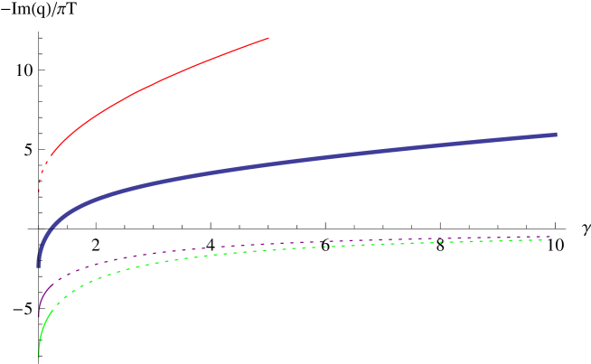
In Fig. (8) we show several branches of $q_{n}(v)$ obtained by these methods. It is interesting to note that a good approximation to the main branch is given by

$${\frac{iq}{\pi T}=4\left(\frac{3}{2}\right)^{\frac{1}{4}}\sqrt{\gamma}\left(v-\frac{1}{\sqrt{3}}\right)\;.}$$

(141)

A better approximation can be found by including more parameters in the fit. Including one more parameter, the curve

$${\frac{iq}{\pi T}=\sqrt{\gamma}\frac{1-v\sqrt{3}}{Fv+G}\;,}$$

(142)

where

$${F=\frac{1}{2}\left(\frac{3}{2}\right)^{3/4}(2^{1/4}-1)^{2}\;,\quad G=-\frac{3^{1/4}(1+2^{1/2}-2^{3/4})}{2^{5/4}}\;,}$$

(143)

gives a better approximation close to the speed of sound and the large $\gamma$ asymptotics.

These approximations can also be used to obtain an approximate function $\omega^{\prime}(q^{\prime})$ (the dispersion law) for the sound waves. Transforming to the unboosted frame and using $v=-\frac{\omega^{\prime}}{q^{\prime}}$, we find that the approximation (141) provides us with the following implicit equation for $\omega^{\prime}(q^{\prime})$:

$${q^{\prime}(q^{\prime 2}-\omega^{\prime 2})^{3/2}=16\left(\frac{3}{2}\right)^{\frac{1}{2}}\left(\omega^{\prime}+\frac{q^{\prime}}{\sqrt{3}}\right)\;.}$$

(144)

The other fit can also be used in this way, but the resulting equation is more complicated and we omit it here.

Figure 8: Imaginary parts of $q/(\pi T)$ versus $\gamma=\frac{1}{\sqrt{1-v^{2}}}$ are plotted. The main branch crosses $0$ at the speed of sound. The dotted sections of the curves denote unphysical values of $q$—those that are discarded as they correspond to perturbations growing exponentially at the respective asymptotic infinities. The solid sections denote physical values (corresponding to $-\mathop{\rm Im}\nolimits(q)<0$ for subsonic $\gamma$ and $-\mathop{\rm Im}\nolimits(q)>0$ for supersonic). The asymptotics for $\gamma\rightarrow\infty$ for the main branch and the one above it are discussed in section (4.3.4).

5 Discussion

In this work we have used the AdS/CFT correspondence to study shock waves propagating in a strongly coupled plasma. Shock waves appear quite generically when the motion of the fluid is supersonic and produce dissipation and drag even for zero viscosity. In the case of ideal fluids they are associated with surfaces where the velocity and pressure are discontinuous. The discontinuity indicates a failure of the hydrodynamic approximation and should generically be resolved by a microscopic description of the system which, in this context, is provided by the dual gravity description. An exception is the case of weak shocks, which propagate close to the speed of sound, where the inclusion of dissipation, namely, viscosity, resolves the shock. In this case, the dual metric can be found using an expansion in the strength of the shock. On the other hand, strong shocks are beyond the hydrodynamic approximation. They can only be resolved by finding the dual gravity solution which should be a smooth wave propagating without deformation on the horizon of the black hole. Far from the shock, the solution differs slightly from a boosted black hole which allows for a perturbative study of the solution. In particular, we have computed, in the rest frame of the shock, the exponential tail of the solution, namely, the width or penetration depth of the shock. It is a function of the velocity, which we have determined numerically. In particular, when the speed of the incoming fluid approaches the speed of light, the penetration depth ahead of the shock goes to zero as the inverse square root of the gamma factor, $\ell\sim\gamma^{-\frac{1}{2}}$. Since the length scale goes to zero, this scaling exponent is an ultraviolet property of the theory, as can also be seen from the bulk calculation, where the exponent is determined by the properties of the metric near the boundary. It would be of interest for future work to establish the value of this exponent for other backgrounds in the context of AdS/CFT or perhaps even directly from perturbative gauge theory calculations, for example, in QCD. More generically, since shock waves probe microscopic properties of the system, they are an ideal tool to study the transition from the microscopic to an effective hydrodynamic description. For example, we have shown that, for strong shocks, the dependence of the penetration depth on the velocity of the incoming fluid is not correctly reproduced either by second order hydrodynamics or by the Israel-Stewart theory. It is possible to encode our results into effective linearized hydrodynamics of the type proposed in [58], but with effective viscosity given by a numerically determined function of $\omega^{\prime}$ and $q^{\prime}$. The linearized description, however, is valid only far from the shock. It would be interesting to see if an improved effective description exists that can correctly capture the main properties of shock waves in the nonlinear region.

Although we have understood several basic properties of shock waves in the context of AdS/CFT, there are many interesting questions that we have not addressed here and would be interesting to pursue. One important question is if the full solutions dual to shock waves can be found analytically or by numerical methods. They are interesting objects in gravity since they correspond to black branes with different asymptotic temperatures on the two sides of the wave. Such waves propagate without deformation and generate entropy by expanding the area of the horizon. Perhaps they are quite a generic phenomenon not restricted only to examples appearing in the context of AdS/CFT. Other, perhaps simpler problems to consider are related to the introduction of dynamical quarks by means of probe branes [65] in the background of the shock. A shock should appear on the brane giving rise to a force on quarks and meson emission from the shock. Finally, the introduction of dynamical quarks can also provide a closer point of contact with the quark-gluon plasma experiments at RHIC where generation of a Mach cone by a heavy quark propagating in the plasma has been recently suggested [66]. For that reason, it would be of great interest to understand the conditions under which a moving quark generates a strong shock such as the one studied in the present paper.

6 Acknowledgements

We are grateful to Denes Molnar and Fuqiang Wang for suggestions and discussions. This work was supported in part by DOE under grant DE-FG02-91ER40681. The work of M.K. was also supported in part by the Alfred P. Sloan Foundation and by NSF under grant PHY-0805948.

Appendix A The equations of motion for the perturbations

In this appendix we derive the equations of motion for various perturbations of the metric. The background metric is given by

$${ds^{2}_{0}=r^{2}\eta_{\mu\nu}dx^{\mu}dx^{\nu}+\frac{r_{0}^{4}}{r^{2}}(dt\frac{1}{\sqrt{1-v^{2}}}-dx\frac{v}{\sqrt{1-v^{2}}})^{2}+\frac{dr^{2}}{r^{2}(1-r_{0}^{4}/r^{4})}\,,}$$

(145)

and the perturbation by

$${ds^{2}_{1}=r^{2}e^{iqx}\left(H_{00}dt^{2}+H_{11}dx^{2}+2H_{01}dtdx+H(dy^{2}+dz^{2})\right)\;.}$$

(146)

There are seven independent equations coming from

$${\tilde{G}_{MN}=R_{MN}+4g_{MN}=0\;.}$$

(147)

We form the linear combination

$${\mathcal{L}=A^{MN}\tilde{G}_{MN}\;,}$$

(148)

where the only non zero entries for the $A$ matrix are the linearly independent equations, which are the $rr,rt,rx,tt,xx,yy,xt$ components of $\tilde{G}_{MN}$ . After choosing four entries for $A_{MN}$, namely $A_{rr},A_{rx},A_{xx},A_{yy}$, one can eliminate $H_{01},H_{11}$ and their derivatives from $\mathcal{L}$. Only four constants are needed since two of the equations are first order. After this operation $\mathcal{L}$ is a function of only $H_{00},H$ and their derivatives. One cannot use the three remaining constants to eliminate one of the functions and it’s derivatives. The reason is that only two constants are free, the third one can be thought of as an overall rescaling of $\mathcal{L}$ and there are three coefficients to eliminate, the three factors multiplying $H,H^{\prime},H^{\prime\prime}$. A redefinition

$${H_{00}(r)=Z(r)-g(r)H(r)\;,}$$

(149)

and choosing $g(r)$ such that the coefficient of $H^{\prime\prime}$ vanishes allows us to write a decoupled equation for $Z(r)$. With the choice of

$${g(r)=1+\frac{r_{h}^{4}}{r^{4}}\frac{1}{1-v^{2}}\;,}$$

(150)

the final equation for $Z(r)$ is

$${Z^{\prime\prime}(r)+Z^{\prime}(r)}$$

(151)

This equation coincides with the equation for the sound pole [59] when one boosts to the frame where the black hole is moving. Now we can trace back the equations and find the equations of motion for the rest of the perturbation components. Tracing back the procedure to derive the equation for $Z(r)$ we find that

$${H^{\prime}(r)=H(r)\frac{2r_{h}^{4}}{r(r^{4}-r_{h}^{4})}-Z^{\prime}(r)\frac{r^{4}(1-v^{2})}{r_{h}^{4}-3r^{4}(1-v^{2})}+Z(r)\frac{2r^{3}r_{h}^{4}(1-v^{2})}{(r^{4}-r_{h}^{4})(r_{h}^{4}-3r^{4}(1-v^{2}))}\;,}$$

(152)

$${H_{00}^{\prime}(r)=H_{00}(r)}$$

(153)

We can treat the $Z(r),Z^{\prime}(r)$ terms as a source since $Z(r)$ satisfies a decoupled equation. For the last two perturbations $H_{01},H_{11}$ it is easier to define a linear combination of them

$${\tilde{H}(r)=vH_{11}(r)+2H_{01}(r)\;.}$$

(154)

Treating terms containing $H(r),Z(r)$ as sources $\tilde{H}$ satisfies

$${\tilde{H}^{\prime}(r)=}$$

(155)

Having determined $\tilde{H}(r)$ the last two perturbations satisfy

$${H_{01}^{\prime}(r)=}$$

(156)

$${H_{11}^{\prime}(r)=}$$

(157)

We can now find the asymptotic behavior for all perturbations close to the horizon and close to the boundary. The results are summarized in table (1).

	$r\rightarrow\infty$	$r\rightarrow r_{h}$	$r\rightarrow r_{f}$
$Z(r)$	$r^{-4}$	$(r-r_{h})^{-i\frac{qv}{4r_{h}\sqrt{(1-v^{2})}}}$	$\zeta_{0}+\zeta_{1}(r-r_{f})+\zeta_{2}(r-r_{f})^{2}+\cdots$
$H_{00}(r)$	$r^{-4}$	$\frac{2v^{2}}{3v^{2}-2}(r-r_{h})^{-i\frac{qv}{4r_{h}\sqrt{(1-v^{2})}}}$, $v<\sqrt{\frac{2}{3}}$	$h^{(0)}_{0}+h^{(0)}_{1}(r-r_{f})+\cdots$
$H(r)$	$r^{-4}$	$\frac{1-v^{2}}{3v^{2}-2}(r-r_{h})^{-i\frac{qv}{4r_{h}\sqrt{(1-v^{2})}}}$, $v<\sqrt{\frac{2}{3}}$	$h_{0}+h_{1}(r-r_{f})+\cdots$
		$\tilde{C}_{1}\sqrt{r-r_{h}}$, $v\geq\sqrt{\frac{2}{3}}$
$\tilde{H}(r)$	$r^{-9}$	$-\frac{2iv(-iqv+2(1-2v^{2})\sqrt{1-v^{2}}-q^{2}(1-v^{2})^{3/2})}{(3v^{2}-2)(qv-4i\sqrt{1-v^{2}})}\cdot$	$\tilde{h}_{0}+\tilde{h}_{1}(r-r_{f})+\cdots$
		$\cdot(r-r_{h})^{-i\frac{qv}{4r_{h}\sqrt{(1-v^{2})}}}$, $v<\sqrt{\frac{2}{3}}$
		$\tilde{C}_{2}\sqrt{r-r_{h}}$ ,$v\geq\sqrt{\frac{2}{3}}$
$H_{01}(r)$	$r^{-9}$		$h^{(01)}_{0}+h^{(01)}_{1}(r-r_{f})+\cdots$
$H_{11}(r)$	$r^{-9}$		$h^{(11)}_{0}+h^{(11)}_{1}(r-r_{f})+\cdots$

Table 1: The behavior of the perturbations close to the boundary, the horizon and the pole of the equation (151) is given. Here, $r_{f}=\frac{1}{3^{1/4}}\frac{r_{h}}{(1-v^{2})^{1/4}}$ is the location of the pole of (151). The boundary conditions for the perturbations at the boundary $r\rightarrow\infty$ are that the metric is unchanged from the Minkowski metric. At the horizon the condition is that the asymptotic behavior corresponds to an infalling graviton in the unboosted black hole. In the linearized approximation the overall scaling factor does not appear and we only show the power law behavior. The normalization of the perturbations close to the horizon are relative to the normalization of $Z(r)$. The normalization of $Z(r)$ is taken to be $1$ for the factor multiplying $(r-r_{h})^{-i\frac{qv}{4r_{h}\sqrt{(1-v^{2})}}}$. For $v\geq\sqrt{\frac{2}{3}}$ the relative coefficients $\tilde{C}_{1,2}$ are not computed. The asymptotic behavior of $H_{01},H_{11}$ is not shown for brevity but can be easily inferred from (156)-(157).

The behavior of $H_{01}$ and $H_{11}$ close to the boundary are consistent with the equations of motion for the boundary stress energy tensor. The last can be rewritten as

$${\delta T^{01}=0\;,\quad\delta T^{11}=0\;,}$$

(158)

where $\delta T^{\mu\nu}$ denote the perturbations away from the ideal boosted fluid stress energy tensor. From the $AdS/CFT$ dictionary we know that

$${\delta T^{01}=\lim_{r\rightarrow\infty}r^{2}H^{01}(r)=0\;,\quad\delta T^{00}=\lim_{r\rightarrow\infty}r^{2}H^{11}(r)=0\;.}$$

(159)

in agreement with (158).

Appendix B Expansion near the boundary

Given a conserved boundary energy momentum tensor the boundary conditions for an asymptotic AdS metric are fixed. There is a procedure [67] that allows one to find such metric expanded in powers of $\frac{1}{r}$ where $r$ is the radial coordinate in the Poincare AdS patch, such that $r=0$ is the horizon and $r=\infty$ the boundary. In our case the procedure simplifies. We fix the energy momentum tensor to be

$$T^{tt}=\varepsilon(x),\ \ T^{tx}=C_{1},\ \ T^{xx}=C_{2},\ \ T^{yy}=T^{zz}=\frac{1}{2}\varepsilon-\frac{1}{2}C_{2}\;,$$ (160)

which is obviously conserved ($\partial_{\mu}T^{\mu\nu}=0$). The energy density $\varepsilon(x)$ has to be computed from the hydrodynamic equations or a guess can be made. In any case this fixes the boundary condition and allows us to extend the metric as:

$$g_{tt} = \framebox{$\displaystyle-r^{2}-\frac{\varepsilon}{r^{2}}$}+\frac{\varepsilon^{\prime\prime}}{12r^{4}}+\frac{1}{r^{6}}\left(\frac{\varepsilon C_{2}}{24}-\frac{7\varepsilon^{2}}{16}+\frac{C_{2}^{2}}{16}+\frac{5C_{1}^{2}}{48}-\frac{\varepsilon^{iv}}{384}\right)$$ (161)

$$+\frac{1}{r^{8}}\left(\frac{3}{40}\varepsilon\varepsilon^{\prime\prime}-\frac{7}{360}C_{2}\varepsilon^{\prime\prime}-\frac{1}{480}\varepsilon^{\prime}{}^{2}+\frac{1}{23040}\varepsilon^{vi}\right)+\frac{1}{r^{10}}\left(\frac{C_{2}^{2}\varepsilon}{48}-\frac{29\varepsilon^{\prime\prime}{}^{2}}{9216}+\frac{77C_{2}\varepsilon^{iv}}{69210}-\frac{11\varepsilon\varepsilon^{iv}}{4608}\right.$$

$$\left.-\frac{\varepsilon^{viii}}{2211840}+\frac{11C_{1}^{2}\varepsilon}{144}+\frac{C_{1}^{2}C_{2}}{24}+\frac{C_{2}\varepsilon^{2}}{72}-\frac{7\varepsilon^{3}}{48}+\frac{\varepsilon^{\prime}\varepsilon^{\prime\prime\prime}}{4608}\right)+{\cal O}\left(\frac{1}{r^{12}}\right)\;,$$

$$2g_{tz} = \framebox{$\displaystyle\frac{C_{1}}{r^{2}}$}+\frac{C_{1}(C_{2}+\varepsilon)}{2r^{6}}-\frac{1}{20}\frac{C_{1}\varepsilon^{\prime\prime}}{r^{8}}+\frac{1}{r^{10}}\left(\frac{C_{1}\varepsilon^{iv}}{576}-\frac{5C_{1}^{3}}{144}+\frac{7C_{1}C_{2}^{2}}{48}+\frac{11C_{1}C_{2}\varepsilon}{72}+\frac{7C_{1}\varepsilon^{2}}{48}\right)$$ (162)

$$-\frac{C_{1}}{161280r^{12}}\left(5\varepsilon^{vi}+48\varepsilon^{\prime}{}^{2}+4512\varepsilon\varepsilon^{\prime\prime}+736C_{2}\varepsilon^{\prime\prime}\right)+{\cal O}\left(\frac{1}{r^{14}}\right)\;.$$

$$g_{xx} = \framebox{$\displaystyle r^{2}+\frac{C_{2}}{r^{2}}$}+\frac{1}{r^{6}}\left(-\frac{C_{2}\varepsilon}{24}-\frac{\varepsilon^{2}}{16}+\frac{7}{16}C_{2}^{2}-\frac{5}{48}C_{1}^{2}\right)+\frac{1}{r^{8}}\left(\frac{1}{240}\varepsilon^{\prime\prime}C_{2}+\frac{1}{80}\varepsilon\varepsilon^{\prime\prime}-\frac{1}{160}\varepsilon^{\prime}{}^{2}\right)$$ (163)

$$+\frac{1}{r^{10}}\left(-\frac{C_{2}^{2}\varepsilon}{72}-\frac{3\varepsilon^{\prime\prime}{}^{2}}{5120}-\frac{C_{2}\varepsilon^{iv}}{7680}-\frac{\varepsilon\varepsilon^{iv}}{2560}-\frac{C_{1}^{2}\varepsilon}{24}-\frac{11C_{1}^{2}C_{2}}{144}+\frac{7C_{2}^{3}}{48}-\frac{C_{2}\varepsilon^{2}}{48}+\frac{\varepsilon^{\prime}\varepsilon^{\prime\prime\prime}}{1536}\right)$$

$$+{\cal O}\left(\frac{1}{r^{12}}\right)\;,$$

$$g_{yy} = g_{zz}=\framebox{$\displaystyle r^{2}-\frac{C_{2}}{2r^{2}}-\frac{\varepsilon}{2r^{2}}$}+\frac{\varepsilon^{\prime\prime}}{24r^{4}}+\frac{1}{r^{6}}\left(\frac{5}{24}C_{2}\varepsilon+\frac{\varepsilon^{2}}{16}+\frac{C_{2}^{2}}{16}+\frac{C_{1}^{2}}{48}-\frac{\varepsilon^{iv}}{768}\right)$$ (164)

$$+\frac{1}{r^{8}}\left(\frac{1}{480}\varepsilon^{\prime}{}^{2}+\frac{1}{46080}\varepsilon^{vi}-\frac{19}{720}C_{2}\varepsilon^{\prime\prime}-\frac{1}{80}\varepsilon\varepsilon^{\prime\prime}\right)+\frac{1}{r^{10}}\left(-\frac{13C_{2}^{2}\varepsilon}{288}+\frac{5\varepsilon^{\prime\prime}{}^{2}}{9216}+\frac{19C_{2}\varepsilon^{iv}}{17280}\right.$$

$$\left.+\frac{\varepsilon\varepsilon^{iv}}{2304}-\frac{\varepsilon^{viii}}{4423680}-\frac{C_{1}^{2}\varepsilon}{288}-\frac{C_{1}^{2}C_{2}}{288}-\frac{C_{2}^{3}}{96}-\frac{13C_{2}\varepsilon^{2}}{288}-\frac{\varepsilon^{3}}{96}-\frac{\varepsilon^{\prime}\varepsilon^{\prime\prime\prime}}{4608}\right)+{\cal O}\left(\frac{1}{r^{12}}\right)\;,$$

where the boxed terms are fixed by the boundary conditions and the rest can be computed from solving the Einstein equations. In the absence of an exact metric for the shock wave, this expansion provides more information about it and could possible be used in the future as a check of given solutions and as a starting point for a numerical method. Although we show a few terms, it should be noted that using a computer algebra program we found easily the expansion up to order $\frac{1}{r^{30}}$ although it is too lengthy to display here. These are enough terms to attempt a reconstruction of the metric using Padé approximants. The condition that determines the function $\varepsilon(x)$ then comes from demanding that the metric does not develop a singularity. In fact, in Fefferman-Graham coordinates the $AdS$-Schwarzschild black hole metric becomes degenerate at the horizon and one cannot go beyond the horizon in these coordinates.

References

- [1] J. M. Maldacena, “The large N limit of superconformal field theories and supergravity,” Adv. Theor. Math. Phys. 2 (1998) 231–252, hep-th/9711200.
- [2] S. S. Gubser, I. R. Klebanov, and A. M. Polyakov, “Gauge theory correlators from non-critical string theory,” Phys. Lett. B428 (1998) 105–114, hep-th/9802109.
- [3] E. Witten, “Anti-de Sitter space and holography,” Adv. Theor. Math. Phys. 2 (1998) 253–291, hep-th/9802150.
- [4] O. Aharony, S. S. Gubser, J. M. Maldacena, H. Ooguri, and Y. Oz, “Large N field theories, string theory and gravity,” Phys. Rept. 323 (2000) 183–386, hep-th/9905111.
- [5] G. ’t Hooft, “A planar diagram theory for strong interactions,” Nucl. Phys. B72 (1974) 461.
- [6] D. T. Son and A. O. Starinets, “Viscosity, Black Holes, and Quantum Field Theory,” Ann. Rev. Nucl. Part. Sci. 57 (2007) 95–118, 0704.0240.
- [7] E. Shuryak, “Physics of Strongly coupled Quark-Gluon Plasma,” Prog. Part. Nucl. Phys. 62 (2009) 48–101, 0807.3033.
- [8] T. Schafer and D. Teaney, “Nearly Perfect Fluidity: From Cold Atomic Gases to Hot Quark Gluon Plasmas,” Rept. Prog. Phys. 72 (2009) 126001, 0904.3107.
- [9] S. S. Gubser and A. Karch, “From gauge-string duality to strong interactions: a Pedestrian’s Guide,” Ann. Rev. Nucl. Part. Sci. 59 (2009) 145–168, 0901.0935.
- [10] S. S. Gubser, S. S. Pufu, F. D. Rocha, and A. Yarom, “Energy loss in a strongly coupled thermal medium and the gauge-string duality,” 0902.4041.
- [11] L. D. Landau, “On the multiparticle production in high-energy collisions,” Izv. Akad. Nauk SSSR Ser. Fiz. 17 (1953) 51–64.
- [12] S. S. Gubser, S. S. Pufu, and A. Yarom, “Entropy production in collisions of gravitational shock waves and of heavy ions,” Phys. Rev. D78 (2008) 066014, 0805.1551.
- [13] E. Avsar, E. Iancu, L. McLerran, and D. N. Triantafyllopoulos, “Shockwaves and deep inelastic scattering within the gauge/gravity duality,” JHEP 11 (2009) 105, 0907.4604.
- [14] G. Beuf, “Gravity dual of N=4 SYM theory with fast moving sources,” Phys. Lett. B686 (2010) 55–58, 0903.1047.
- [15] J. L. Albacete, Y. V. Kovchegov, and A. Taliotis, “Modeling Heavy Ion Collisions in AdS/CFT,” JHEP 07 (2008) 100, 0805.2927.
- [16] P. C. Aichelburg and R. U. Sexl, “On the Gravitational field of a massless particle,” Gen. Rel. Grav. 2 (1971) 303–312.
- [17] T. Dray and G. ’t Hooft, “The Gravitational Shock Wave of a Massless Particle,” Nucl. Phys. B253 (1985) 173.
- [18] M. Hotta and M. Tanaka, “Shock wave geometry with nonvanishing cosmological constant,” Class. Quant. Grav. 10 (1993) 307–314.
- [19] K. Sfetsos, “On gravitational shock waves in curved space-times,” Nucl. Phys. B436 (1995) 721–746, hep-th/9408169.
- [20] J. Podolsky and J. B. Griffiths, “Impulsive waves in de Sitter and anti-de Sitter space- times generated by null particles with an arbitrary multipole structure,” Class. Quant. Grav. 15 (1998) 453–463, gr-qc/9710049.
- [21] G. T. Horowitz and N. Itzhaki, “Black holes, shock waves, and causality in the AdS/CFT correspondence,” JHEP 02 (1999) 010, hep-th/9901012.
- [22] R. Emparan, “Exact gravitational shockwaves and Planckian scattering on branes,” Phys. Rev. D64 (2001) 024025, hep-th/0104009.
- [23] G. Arcioni, S. de Haro, and M. O’Loughlin, “Boundary description of Planckian scattering in curved spacetimes,” JHEP 07 (2001) 035, hep-th/0104039.
- [24] W. A. Horowitz, “Shock Treatment: Heavy Quark Energy Loss in a Novel AdS/CFT Geometry,” Nucl. Phys. A830 (2009) 773c–776c, 0907.4845.
- [25] W. A. Horowitz and Y. V. Kovchegov, “Shock Treatment: Heavy Quark Drag in a Novel AdS Geometry,” Phys. Lett. B680 (2009) 56–61, 0904.2536.
- [26] J. J. Friess, S. S. Gubser, G. Michalogiorgakis, and S. S. Pufu, “The stress tensor of a quark moving through N = 4 thermal plasma,” Phys. Rev. D75 (2007) 106003, hep-th/0607022.
- [27] S. S. Gubser, S. S. Pufu, and A. Yarom, “Energy disturbances due to a moving quark from gauge- string duality,” JHEP 09 (2007) 108, 0706.0213.
- [28] S. S. Gubser, S. S. Pufu, and A. Yarom, “Sonic booms and diffusion wakes generated by a heavy quark in thermal AdS/CFT,” Phys. Rev. Lett. 100 (2008) 012301, 0706.4307.
- [29] P. M. Chesler and L. G. Yaffe, “The wake of a quark moving through a strongly-coupled supersymmetric Yang-Mills plasma,” Phys. Rev. Lett. 99 (2007) 152001, 0706.0368.
- [30] P. M. Chesler and L. G. Yaffe, “The stress-energy tensor of a quark moving through a strongly-coupled N=4 supersymmetric Yang-Mills plasma: comparing hydrodynamics and AdS/CFT,” Phys. Rev. D78 (2008) 045013, 0712.0050.
- [31] W. Scheid, H. Muller, and W. Greiner, “Nuclear Shock Waves in Heavy-Ion Collisions,” Phys. Rev. Lett. 32 (1974) 741–745.
- [32] H. G. Baumgardt et al., “Shock Waves and MACH Cones in Fast Nucleus-Nucleus Collisions,” Z. Phys. A273 (1975) 359–371.
- [33] H. H. Gutbrod, A. M. Poskanzer, and H. G. Ritter, “Plastic ball experiments,” Rept. Prog. Phys. 52 (1989) 1267.
- [34] H. H. Gutbrod et al., “Squeezeout of nuclear matter as a function of projectile energy and mass,” Phys. Rev. C42 (1990) 640–651.
- [35] STAR Collaboration, J. Adams et al., “Transverse momentum and collision energy dependence of high p(T) hadron suppression in Au + Au collisions at ultrarelativistic energies,” Phys. Rev. Lett. 91 (2003) 172302, nucl-ex/0305015.
- [36] PHENIX Collaboration, A. Adare et al., “Suppression pattern of neutral pions at high transverse momentum in Au+Au collisions at and constraints on medium transport coefficients,” Phys. Rev. Lett. 101 (2008) 232301, 0801.4020.
- [37] STAR Collaboration, F. Wang, “Measurement of jet modification at RHIC,” J. Phys. G30 (2004) S1299–S1304, nucl-ex/0404010.
- [38] STAR Collaboration, J. Adams et al., “Distributions of charged hadrons associated with high transverse momentum particles in p p and Au + Au collisions at s(NN)**(1/2) = 200-GeV,” Phys. Rev. Lett. 95 (2005) 152301, nucl-ex/0501016.
- [39] PHENIX Collaboration, S. S. Adler et al., “Modifications to di-jet hadron pair correlations in Au + Au collisions at s(NN)**(1/2) = 200-GeV,” Phys. Rev. Lett. 97 (2006) 052301, nucl-ex/0507004.
- [40] STAR Collaboration, J. G. Ulery, “Two- and three-particle jet correlations from STAR,” Nucl. Phys. A774 (2006) 581–584, nucl-ex/0510055.
- [41] PHENIX Collaboration, N. N. Ajitanand, “Extraction of jet topology using three particle correlations,” Nucl. Phys. A783 (2007) 519–522, nucl-ex/0609038.
- [42] PHENIX Collaboration, A. Adare et al., “Dihadron azimuthal correlations in Au+Au collisions at ,” Phys. Rev. C78 (2008) 014901, 0801.4545.
- [43] H. Stoecker, “Collective Flow signals the Quark Gluon Plasma,” Nucl. Phys. A750 (2005) 121–147, nucl-th/0406018.
- [44] J. Ruppert and B. Muller, “Waking the colored plasma,” Phys. Lett. B618 (2005) 123–130, hep-ph/0503158.
- [45] V. Koch, A. Majumder, and X.-N. Wang, “Cherenkov Radiation from Jets in Heavy-ion Collisions,” Phys. Rev. Lett. 96 (2006) 172302, nucl-th/0507063.
- [46] J. Casalderrey-Solana, E. V. Shuryak, and D. Teaney, “Conical flow induced by quenched QCD jets,” J. Phys. Conf. Ser. 27 (2005) 22–31, hep-ph/0411315.
- [47] I. Bouras et al., “Relativistic shock waves in viscous gluon matter,” Phys. Rev. Lett. 103 (2009) 032301, 0902.1927.
- [48] I. Bouras et al., “Relativistic Shock Waves and Mach Cones in Viscous Gluon Matter,” 1004.4615.
- [49] L. D. Landau and E. M. Lifshitz, Fluid Mechanics. Elsevier, Oxford GB, 2nd ed., 2009.
- [50] S. Bhattacharyya, V. E. Hubeny, S. Minwalla, and M. Rangamani, “Nonlinear Fluid Dynamics from Gravity,” JHEP 02 (2008) 045, 0712.2456.
- [51] G. Policastro, D. T. Son, and A. O. Starinets, “The shear viscosity of strongly coupled N = 4 supersymmetric Yang-Mills plasma,” Phys. Rev. Lett. 87 (2001) 081601, hep-th/0104066.
- [52] R. Baier, P. Romatschke, D. T. Son, A. O. Starinets, and M. A. Stephanov, “Relativistic viscous hydrodynamics, conformal invariance, and holography,” JHEP 04 (2008) 100, 0712.2451.
- [53] M. Natsuume and T. Okamura, “Causal hydrodynamics of gauge theory plasmas from AdS/CFT duality,” Phys. Rev. D77 (2008) 066014, 0712.2916.
- [54] R. Loganayagam, “Entropy Current in Conformal Hydrodynamics,” JHEP 05 (2008) 087, 0801.3701.
- [55] S. Bhattacharyya et al., “Local Fluid Dynamical Entropy from Gravity,” JHEP 06 (2008) 055, 0803.2526.
- [56] W. Israel, “Nonstationary irreversible thermodynamics: A Causal relativistic theory,” Ann. Phys. 100 (1976) 310–331.
- [57] W. Israel and J. M. Stewart, “Transient relativistic thermodynamics and kinetic theory,” Ann. Phys. 118 (1979) 341–372.
- [58] M. Lublinsky and E. Shuryak, “Improved Hydrodynamics from the AdS/CFT,” Phys. Rev. D80 (2009) 065026, 0905.4069.
- [59] P. K. Kovtun and A. O. Starinets, “Quasinormal modes and holography,” Phys. Rev. D72 (2005) 086009, hep-th/0506184.
- [60] E. Berti, V. Cardoso, and A. O. Starinets, “Quasinormal modes of black holes and black branes,” Class. Quant. Grav. 26 (2009) 163001, 0905.2975.
- [61] G. Arfken and H. Weber, Mathematical methods for physicists. Elsevier, 2005.
- [62] U. H. Danielsson, E. Keski-Vakkuri, and M. Kruczenski, “Vacua, Propagators, and Holographic Probes in AdS/CFT,” JHEP 01 (1999) 002, hep-th/9812007.
- [63] E. Witten, “Anti-de Sitter space, thermal phase transition, and confinement in gauge theories,” Adv. Theor. Math. Phys. 2 (1998) 505–532, hep-th/9803131.
- [64] R. C. Brower, S. D. Mathur, and C.-I. Tan, “Glueball Spectrum for QCD from AdS Supergravity Duality,” Nucl. Phys. B587 (2000) 249–276, hep-th/0003115.
- [65] F. Bigazzi et al., “D3-D7 Quark-Gluon Plasmas,” JHEP 11 (2009) 117, 0909.2865.
- [66] STAR Collaboration, B. I. Abelev et al., “Indications of Conical Emission of Charged Hadrons at RHIC,” Phys. Rev. Lett. 102 (2009) 052302, 0805.0622.
- [67] S. de Haro, S. N. Solodukhin, and K. Skenderis, “Holographic reconstruction of spacetime and renormalization in the AdS/CFT correspondence,” Commun. Math. Phys. 217 (2001) 595–622, hep-th/0002230.