On the Interpretation of Supernova Light Echo Profiles and Spectra

Abstract

The light echo systems of historical supernovae in the Milky Way and local group galaxies provide an unprecedented opportunity to reveal the effects of asymmetry on observables, particularly optical spectra. Scattering dust at different locations on the light echo ellipsoid witnesses the supernova from different perspectives and the light consequently scattered towards Earth preserves the shape of line profile variations introduced by asymmetries in the supernova photosphere. However, the interpretation of supernova light echo spectra to date has not involved a detailed consideration of the effects of outburst duration and geometrical scattering modifications due to finite scattering dust filament dimension, inclination, and image point-spread function and spectrograph slit width. In this paper, we explore the implications of these factors and present a framework for future resolved supernova light echo spectra interpretation, and test it against Cas A and SN 1987A light echo spectra. We conclude that the full modeling of the dimensions and orientation of the scattering dust using the observed light echoes at two or more epochs is critical for the correct interpretation of light echo spectra. Indeed, without doing so one might falsely conclude that differences exist when none are actually present.

1. Introduction

The first light echoes (LEs) were discovered around Nova Persei 1901 (Ritchey, 1901a, b, 1902; Kapteyn, 1902). Since then, LEs (whereby we mean a simple scattering echo rather than fluorescence or dust re-radiation) have been seen in the Galactic Nova Sagittarii 1936 (Swope, 1940) and the eruptive variable V838 Monocerotis (e.g., Bond et al., 2003). LEs have also been observed from extragalactic supernovae (SNe), with SN 1987A (Kunkel87) being the most famous case (Crotts, 1988; Suntzeff et al., 1988; Bond et al., 1990; Xu et al., 1995; Sugerman et al., 2005a, b; Newman & Rest, 2006), but also including SNe 1991T (Schmidt et al., 1994; Sparks et al., 1999), 1993J (Sugerman & Crotts, 2002; Liu et al., 2003), 1995E (Quinn et al., 2006), 1998bu (Cappellaro et al., 2001), 2002hh (Meikle et al., 2006; Welch, 2007), 2003gd (Sugerman, 2005; Van Dyk et al., 2006), and 2006X (Wang et al., 2008).

The suggestion that historical SNe might be studied by their scattered LEs was first made by Zwicky (1940) and attempted by van den Bergh (1965, 1966). The first LEs of centuries-old SNe were discovered in the Large Magellanic Cloud (LMC) (Rest et al., 2005b). They found three LE complexes associated with three small and therefore relatively young SN remnants (SNRs) in the LMC which were subsequently dated as being between 400–1000 years old using the LMC distance and LE feature positions and apparent motions (Rest et al., 2005b). These findings provided the extraordinary opportunity to study the spectrum of the SN light that reached Earth hundreds of years ago and had never been recorded visually or by modern scientific instrumentation. A spectrum of one of the LEs associated with SNR 0509-675 revealed that the reflected LE light came from a high-luminosity SN Ia (Rest et al., 2008a), similar to SN 1991T (Filippenko et al., 1992; Phillips et al., 1992) and SN 1999aa (Garavini et al., 2004) — the first time that an ancient SNe was classified using its LE spectrum. Analysis of ASCA X-ray data of SNR 0509-675 led Hughes et al. (1995) to suggest that this SNR likely came from a SN Ia. Recent analysis of its Chandra X-ray spectra by Badenes et al. (2008) also supported the classification of this object as a high-luminosity SN Ia.

The interpretation of LEs, however, is fraught with subtleties. Krause et al. (2005), for example, identified moving Cas A features (called “infrared echoes” or “IR echoes”) using mid-IR imaging from the Spitzer Space Telescope. IR echoes are the result of dust absorbing the outburst light, warming and re-radiating at longer wavelengths. The main scientific conclusion of Krause et al. (2005) was that most of the IR echoes were caused by a series of recent X-ray outbursts from the compact object in the Cas A SNR based on their apparent motions. However, the analysis was flawed because it did not account for the fact that the apparent motion strongly depends on the inclination of the scattering dust filament (Dwek & Arendt, 2008; Rest11_casamotion). Dwek & Arendt (2008) also showed that X-ray flares are not energetic enough to be the source of these IR echoes, but that instead the LEs must have been generated by an intense and short burst of EUV-UV radiation associated with the break out of the shock through the surface of the Cas A progenitor star. Therefore, the most likely source of all LEs associated with Cas A, both infrared and scattered, is the Cas A SN explosion itself. The need to properly analyze the growing collection of LE spectra is what motivated the present work.

The first scattered LEs of Galactic SNe associated with Tycho’s SN and the Cas A SN were discovered by Rest et al. (2007, 2008b). Contemporaneously, Krause et al. (2008) obtained a spectrum of a scattered optical LE spatially coincident with one of the Cas A IR echoes, and identified the Cas A SN to be of Type IIb. Because Rest et al. (2008b) discovered several LEs with multiple position angles relative to the SNRs, there is a new opportunity for observational SN research — the ability to measure the spectrum of the same SN from several different directions. At any given instant after the SN light has reached an observer by the direct path, an ellipsoidal surface exists where scattered light from the SN may reach the observer, whose arrival to the observer is delayed by the additional path length. Interstellar dust concentrations must lie at one or more locations on the ellipsoid for the scattered LE to be detectable. Since each LE is at a unique position on the ellipsoid, each LE has a unique line of sight to the SN. Therefore, the scattered spectral light can provide spectral information on the asymmetry of the SN photosphere. In the limiting case of dust on the ellipsoid opposite the observer, the spectrum of the scattered LE carries the signature of conditions on the SN hemisphere usually hidden from the observer. As the time since the explosion increases, the scattering ellipsoid surface expands and may intersect additional dust concentrations. We present a framework on how to interpret observed LE spectra depending on the scattering dust properties, seeing, and spectrograph slit width and position.

In this paper, we examine the pitfalls of previous analyses, suggest improvements for future studies, and present the application of our methods to data. In Section 2, we describe how the properties of the scattering dust can cause significant differences to observed LE spectra, and show a specific example of how this has been overlooked in the past. In Section 3, we quantify how observed LE spectra depend on potential differences in dust characteristics (thickness and inclination), as well as observational characteristics (seeing and spectroscopic slit size and orientation). We then apply this framework to observations of Cas A (Section 4) and SN 1987A (Section 5). In Section 6, we discuss how differences in the dust and observing conditions can effect an analysis of LE spectra and suggest future applications of LE observations. We conclude in Section 7.

2. A Case Study: The Krause et al. (2008) Cas A Light Echo Spectrum

A common assumption is that an observed LE spectrum is equivalent to the light-curve weighted integration of the spectra at individual epochs (e.g., Rest et al., 2008a; Krause et al., 2008). However, Figure 1 illustrates how slit width, dust filament width and inclination significantly influence the observed LE spectrum. We consider a LE from a 300-year-old event 10,000 light years away that lasts 150 days (yellow shaded area), with a rising and declining arm of 30 and 120 days, respectively. The peak of the event is indicated with the red line. We place the origin of our coordinate system $\rho,z$ at the source event. The $z$-axis is the distance of the dust to the source event along the line of sight. The $\rho$-axis is in the plane of the sky from the source event to the LE position. The quadratic relation between the parameters $z$, $\rho$, and the time since explosion $t$ is described by the well-known LE equation (Couderc, 1939) (see Section A for details).

The scattering dust filament (brown shaded area) is located at $(\rho,z)=(300,0)$ ly with an inclination of $\alpha=0$^∘ where $\alpha$ is the angle with respect to the plane of the sky (see Equation A3). The dust width is 0.02 ly, 0.2 ly, and 0.6 ly from left to right, respectively. The rightmost panel of Figure 1 shows the flux of the LE that we would observe with these dust filaments versus $\rho$. We denote these as the LE profiles, which essentially are cuts through the LE along the axis pointing toward the source event. In order to be able to directly compare the LE profiles to the dust and LE pulse geometry, we show the flux and $\rho$ as the x- and y-axis, respectively. Note that for very thin dust filaments like the one with $\sigma_{d}=0.02$ ly, the LE profile is the the projected light curve.

A spectroscopic slit with a width of $1\hbox{${}^{\prime\prime}$}$ is indicated with the gray shaded area. In the leftmost panel, the dust filament has a dust width of 0.02 ly (0.006 pc). Only light that is in the intersection of the event pulse, dust, and slit (indicated with the thick black rectangle) contributes to the observed spectra. In this case, only 20% of the event (30 out of 150 days, indicated by the dashed blue lines) contribute to the spectrum. The second panel from the left shows the same example, but this time the dust filament has a width of 0.2 ly (0.06 pc), and $\sim\!\!$ 51% of the event pulse (77 out of 150 days) contributes to the spectrum. Only if the dust width is at least 0.6 ly (0.18 pc) thick (third panel from the left), the full event contributes to the spectrum.

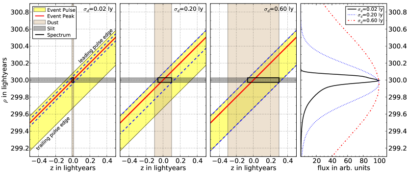
Figure 1.— Illustration of how the dust filament width, $\sigma_{d}$, influences the observed LE spectrum. The yellow shaded area indicates a 300-year-old SN event that lasts 150 days, with a rising and declining arm of 30 and 120 days, respectively. The peak is indicated with a red line. The scattering dust filament (light grey shaded region) is located in the plane of the sky crossing the event position ($z=0.0$ ly), with an inclination of $\alpha=0$^∘. The dust width is 0.02 ly, 0.2 ly, and 0.6 ly from left to right, respectively, and the left panel shows the respective LE profiles. A spectroscopic slit with a width of $1\hbox{${}^{\prime\prime}$}$ is indicated with the dark gray shaded area. Only light that is within the intersection of the event pulse, dust, and slit (indicated with the thick black rectangle) contributes to the observed spectrum. The blue dashed lines indicate which part of the light pulse is probed by the spectrum.

This clearly demonstrates that the observed LE spectrum is not necessarily the full light-curve weighted integrated spectrum when the scattering dust filament is sufficiently thin. The effect of a thin filament of dust on the interpretation of a LE spectrum is best appreciated by considering the difference in persistence of spectral features at early and late time. Naively, one might expect that the faintness of a SN at late times would not result in spectral features from those phases contributing to the integrated spectrum in a significant way. However, in the late nebular phases, most of the flux is typically concentrated in very few lines. The top panel of Figure 2 portrays the spectra of SN 1993J, the very well-observed and prototypical example of the SN IIb class (e.g., Filippenko93; Richmond et al., 1994; Filippenko94; Matheson00), at 6, 39, 88, and 205 days after peak brightness from the bottom to the top, respectively (Jeffery94; Barbon95; Fransson05). During the late phases, a significant fraction of flux is radiated in the [O I] $\lambda\lambda 6300$, 6364 doublet, which completely dominates the spectra for times later than 200 days. The bottom panel shows the light-curve weighted integrated spectra of SN 1993J with different integration limits. The integration limits of these spectra are from 20 days before peak brightness to $P_{\rm max}$, where $P_{\rm max}$ ranges from 5 to 300 days after peak brightness from the bottom to the top. The most significant difference between the integrated spectra with early and late integration limits is the emergence of the [O I] doublet. We use the SN 1993J lightcurve from Richmond96 as weights for the integration.

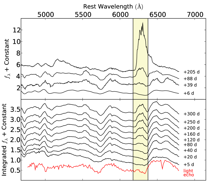
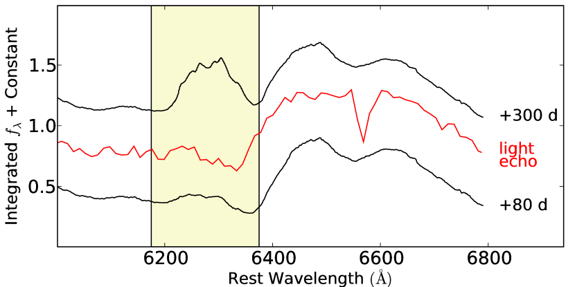
Figure 2.— Top panel: Spectra of SN 1993J at $+6$, $+39$, $+88$, and $+205$ days relative to peak brightness from the bottom to the top, respectively. During the late phases ($\gtrsim 40$ days after peak), a significant fraction of flux is emitted in the [O I] $\lambda\lambda 6300$, 6364 doublet, which dominates the spectra after $\sim\!\!$ 200 days. The [O I] doublet is indicated by the yellow-shaded region. Middle panel: light-curve weighted integrated spectra of SN 1993J. The integration limits of these spectra are from $-20$ days relative to peak brightness to $P_{\max}$, where $P_{\max}$ ranges from $+5$ to $+300$ days from the bottom to the top. The most significant difference between the integrated spectra with early and late integration limits is the emergence of the [O I] doublet. The Cas A LE spectrum of Krause et al. (2008) is shown in red, which does not show a prominent [O I] doublet feature. Bottom panel: light-curve weighted integrated spectra of SN 1993J in the wavelength region near the [O I] doublet and H$\alpha$ features. The integrated spectra have integration limits of $+80$ days and $+300$ days are compared to the Cas A LE spectrum of Krause et al. (2008, red curve). The integrated SN 1993J spectrum with the $+80$ day integration limit is a better fit to the [O I] doublet in the observed Cas A spectrum.

SNe IIb are not unique in this regard. The nebular spectra of all SNe are dominated by strong emission lines. Specifically, SNe Ia have strong [Fe II] and [Fe III] lines, SNe Ib/c have strong [O I], [Mg I], Ca II, and [Ca II] lines, and SNe II have strong hydrogen Balmer lines. See Filippenko (1997) for a review of SN spectroscopy.

The perils of not properly accounting for differences in dust filament thickness are clear — the strength of features in observed LE spectra can be significantly altered by the width of the scattering dust on the sky.

In Figure 2, we display the LE spectrum of Cas A by Krause et al. (2008) in red. This spectrum has a weak [O I] doublet, consistent with the integrated spectra of SN 1993J, but only if integrated until $\sim\!\!$ 80 days after peak brightness. The full integrated spectra of SN 1993J have a much stronger [O I] feature. If the LE spectrum is the full light-curve weighted integrated spectrum of Cas A, then Cas A and SN 1993J have a significant difference at wavelengths near the [O I] feature. The alternative is that the LE spectrum does not contain light from the late-time portion of the SN light curve, i.e., the weighting function is truncated at late times.

In their comparison to the observed Cas A LE, Krause et al. (2008) also used an integrated SN 1993J spectrum — but only integrated to 83 days after peak brightness. This seemingly prudent choice was not explained in the text, but presumably they found this integration time to yield the best comparison. However, this analysis leaves an open question: Was the Cas A SN different from SN 1993J in this regard or are the differences due to the properties of the scattering dust? In the following sections, we attempt to answer this question and its more general counterpart for all LEs.

3. Light Echo Profile Modeling

In Appendix A, we derive that the observed LE profile shape, $P$, strongly depends on the dust thickness, dust inclination, and seeing. We also show that this may have a significant impact on the observed LE spectra (see Appendix B and C). Here we investigate the magnitude of each of these effects on observed LE spectra.

For this analysis, we examine a toy model of a LE that, despite its simplicity in some respects, appears to be representative of actual LE situations. The toy model is a LE from a 300-year-old event 10,000 ly from the observer. For the event light curve, we choose a “sail” shape, with the peak at phase 0.0 years and then decreasing to zero flux at a phase of 0.3 years and $-0.1$ years (see the dotted curves in the right-hand panel of Figures 3 through 7 for a representation of this light curve), sharing the characteristic short rise and long decline of a SN light curve. The scattering dust filament intercepts the LE paraboloid at $(\rho_{0},z_{0})=(300,0)$ ly. For the dust model, we use a dust filament that is locally planar and perpendicular to the $(\rho,z)$ plane, with a boxcar width profile. In the following subsections, we vary the properties of a single parameter while holding the others constant. We are therefore able to determine the effects of each parameter on the observed LE and its spectrum.

3.1. Dust Thickness

As described above, the dust thickness can significantly alter the LE spectrum. Using our toy model, we can quantify this effect.

Figure 3 presents LE profiles, window functions, and effective light curves for the toy model with different dust widths. The left column shows the LE profiles for each dust thickness. The $x$-axis is $\Delta\rho=\rho-\rho_{0}$, where ($\rho_{0},z_{0}$) is the position where the dust intersects with the LE paraboloid at phase 0.0 years of the event. We choose a dust filament inclination of $\alpha=45$^∘, since it is perpendicular to the LE paraboloid and thus most representative of typical inclinations. Centering a $1.0\hbox{${}^{\prime\prime}$}$ spectroscopic slit on the peak of the LE profile, we calculate the associated window function (middle column) and effective light curves (right column), which are simply the light curve convolved with the window function. The different rows show different dust widths.

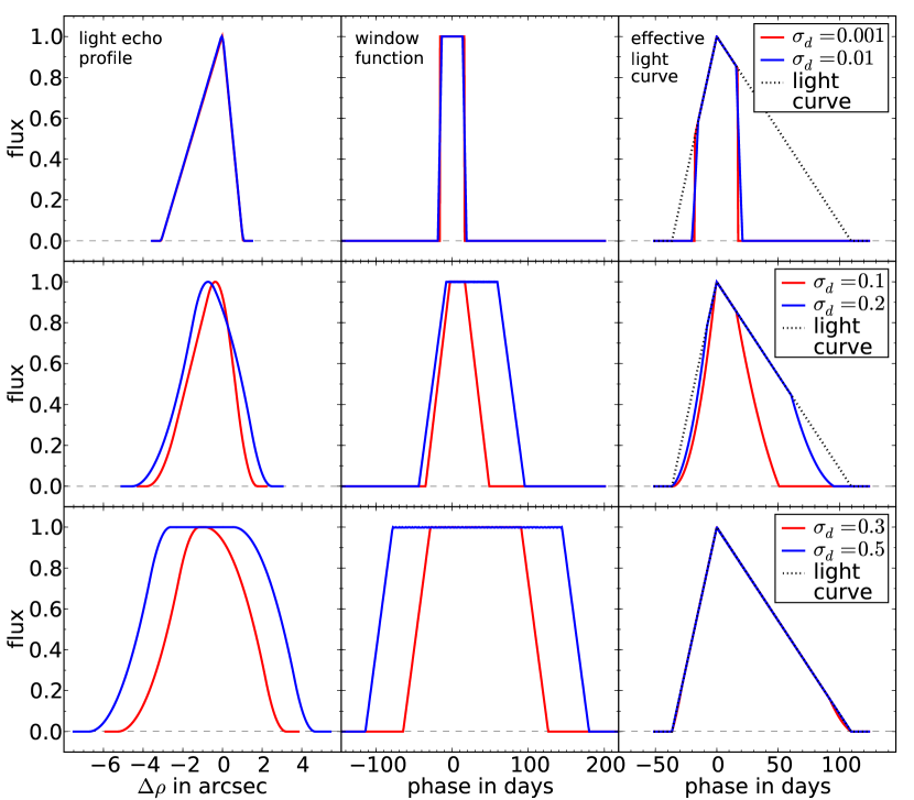
Figure 3.— Modeled LE profiles (left column), window functions (middle column), and effective light curves (right column) for our toy model as a function of dust width. All models in all rows have the same parameters except for the dust width; the separation into three rows is only for clarity. $\Delta\rho$ is with respect to the position where the dust intersects the light pulse. The toy model is a 300-year-old event with a “sail” shape as described in the text. The scattering dust filament intersects the event pulse paraboloid at $z=0.0$, and has an inclination of $\alpha=45$^∘.

There are two distinct regimes where a modest change in the dust width has little effect on the effective light curve or integrated spectrum. The first one is shown in the top panels, where the dust width is so thin that the observed LE profile is effectively the projected initial light curve (corresponding to the left panel of Figure 1). The other limit is a very thick dust sheet (corresponding to the right panel of Figure 1).

In the former case (top row of Figure 3), changing the dust width from $\sigma_{d}=0.001$ ly to $\sigma_{d}=0.01$ ly only marginally modifies the effective light curve. Centering a spectroscopic slit on the LE profile results in a box-car window function, and the effective light curve is truncated to the region near maximum brightness. In the latter case (bottom row of Figure 3), the dust width is large enough that the LE profile is dominated by the dust width. The LE profile has a flat top, and only the edges are impacted by the original light curve profile. Centering a spectroscopic slit on the LE profile results in very wide window functions, and the effective light curve is essentially the same as original light curve (see the right panel of Figure 1 for an illustration).

As we show in Sections 4 and 5, our observations of LEs have been a mixture of both regimes. The middle row of Figure 3 shows the light curves, window functions, and effective light curves for dust widths of $\sigma_{d}=0.1$ ly (0.03 pc) and $\sigma_{d}=0.2$ ly (0.06 pc). The effective light curve is still heavily weighted to the time near maximum, but with increasing dust width the effective light curve slowly transitions to the full light curve.

3.2. Dust Inclination

The dust inclination has a large effect on the LE profile. This is simply a projection effect; as the dust sheet rotates, the projection of the light curve on the sky can change significantly. Turning to our toy model, we quantify this effect.

We fix the dust width to $\sigma_{d}=0.1$ ly. Figure 4 shows modeled LE profiles, window functions, and effective light curves for several examples that only differ by the inclination of the scattering dust filament. As expected, we find that the filament inclination has a profound impact on the LE profile width. For inclinations close to $90$^∘ (see $\alpha=70$^∘ in the top row of Figure 4), the dust filament is aligned along the line of sight, while the light curve projected into $\rho$ space is compressed. Consequently, the window function has large wings, and the effective light curve is very similar to the full light curve. However, for inclination angles corresponding to dust sheets close to the tangent plane of the LE paraboloid (for $z_{0}=0.0$ ly is $-45$^∘), the LE profile subtends a larger angle on the sky (see $\alpha=-30$^∘ in bottom row of Figure 4). As a result, a spectroscopic slit will cover a very small portion of the light curve, and the window function is approximately a box car with a small width.

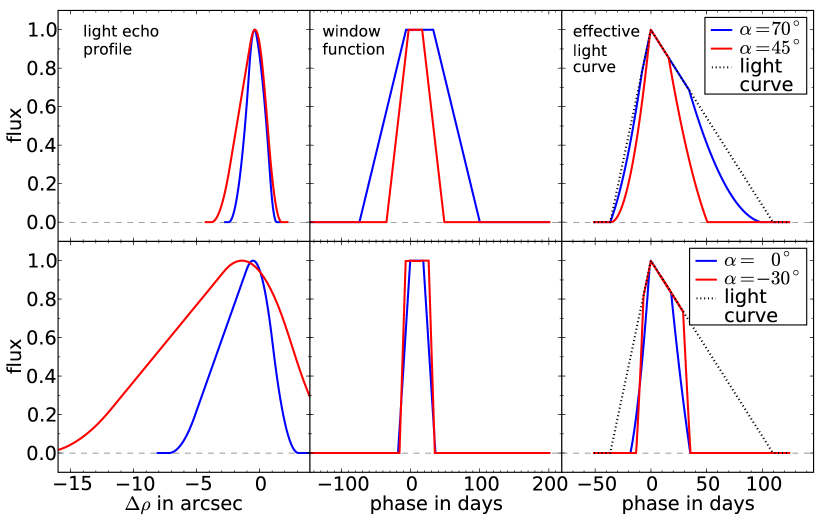
Figure 4.— Same as Figure 3, but for varying dust filament inclinations, $\alpha$, and constant dust width. The width of the dust filament is $\sigma_{d}=0.1$ ly. Note that the LE profile gets “stretched” when the inclination of the dust filament approaches the tangential angle of the LE ellipsoid, which is $\alpha=-45$^∘ for $z=0$ ly.

It is clear that the determining the dust inclination is very important, but fortunately it is straightforward to do so from the observations in cases where the location of the SN and date of outburst are known. In Appendix E and in more detail in Rest et al. (in prep.), we derive the dust inclination from the apparent motion of the LE in difference images, and discuss its sources of uncertainty. We discuss the impact the dust inclination has on the possibility of sampling the spectra within different age intervals for the same SN, as well as the possibility of constraining the SN light curve shape in Section 6.2 and 6.3, respectively.

3.3. Point-Spread Function Size

Observations of resolved sources must always account for the point-spread function (PSF). LEs are no exception since degradation of an image by a large PSF will not only smear the LE across the sky, but will also smear the LE in time. Again, we turn to our toy model, and vary the PSF to determine its effect on the interpretation of LEs.

Figure 5 shows our toy model with dust inclination of $\alpha=45$^∘. We examine a Gaussian PSF with four different full-widths at half-maximum (FWHMs): $0.0\hbox{${}^{\prime\prime}$}$ (corresponding to a $\delta$ function PSF), $0.4\hbox{${}^{\prime\prime}$}$, $1\hbox{${}^{\prime\prime}$}$, and $2\hbox{${}^{\prime\prime}$}$. Each row of Figure 5 represents a different dust thickness, with the top, middle, and bottom rows corresponding to $\sigma_{d}=0.001$, $0.1$, and $0.3$ ly, respectively. For small dust widths ($\lesssim 0.1$ ly), and thus thin LE profiles, the effective light curve depends significantly on the seeing. However, for larger dust widths, the seeing has very little effect on the effective light curve. This insight provides guidance for prioritizing targets for spectroscopic follow-up observations based on the conditions at the telescope.

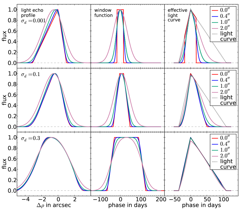
Figure 5.— Same model as in Figure 3, but with varying the dust filament width and seeing. The dust width presented are $\sigma_{d}=0.001$ ly (top row), $\sigma_{d}=0.1$ ly (middle row), and $\sigma_{d}=0.3$ ly (bottom row). Seeing of $0.0\hbox{${}^{\prime\prime}$}$, $0.4\hbox{${}^{\prime\prime}$}$, $1.0\hbox{${}^{\prime\prime}$}$, and $2.0\hbox{${}^{\prime\prime}$}$ is indicated with red, blue, yellow, and green lines, respectively.

3.4. Slit Offset

Thus far, we have assumed for our toy model that the spectroscopic slit was centered on the peak of the LE profile. However, LEs are usually both very faint and extended. Additionally, their apparent motion on the sky makes perfect alignment of a spectroscopic slit unlikely - especially when there is a significant delay between the time of mask preparation and observations. Figure 6 shows the effect of having the slit offset from the LE profile peak. As before, we choose a representative dust inclination of $\alpha=45$^∘, and the three rows, from top-to-bottom, correspond to dust widths of $\sigma_{d}=0.001$, $0.1$, and $0.3$ ly, respectively. The red, blue, and green shaded areas indicate $1\hbox{${}^{\prime\prime}$}$ slits with $0.0\hbox{${}^{\prime\prime}$}$, $-1.1\hbox{${}^{\prime\prime}$}$, and $-2.2\hbox{${}^{\prime\prime}$}$ offsets from the peak, respectively. Clearly a $1\hbox{${}^{\prime\prime}$}$ offset has a significant impact on the effective light curve for all but the thickest dust widths (but even in that case, it could still result in a significant difference if the spectroscopic features in the outburst spectra are changing rapidly with time). Figure 7 shows the same scenario as Figure 6, but with the addition of a $1\hbox{${}^{\prime\prime}$}$ PSF to the model.

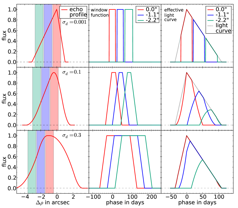
Figure 6.— Same as Figure 3, but with slits that are offset by $0.0\hbox{${}^{\prime\prime}$}$, $-1.1\hbox{${}^{\prime\prime}$}$, and $-2.2\hbox{${}^{\prime\prime}$}$ from the peak of the LE profile. The $1\hbox{${}^{\prime\prime}$}$ slits are indicated with the shaded areas in the left column.

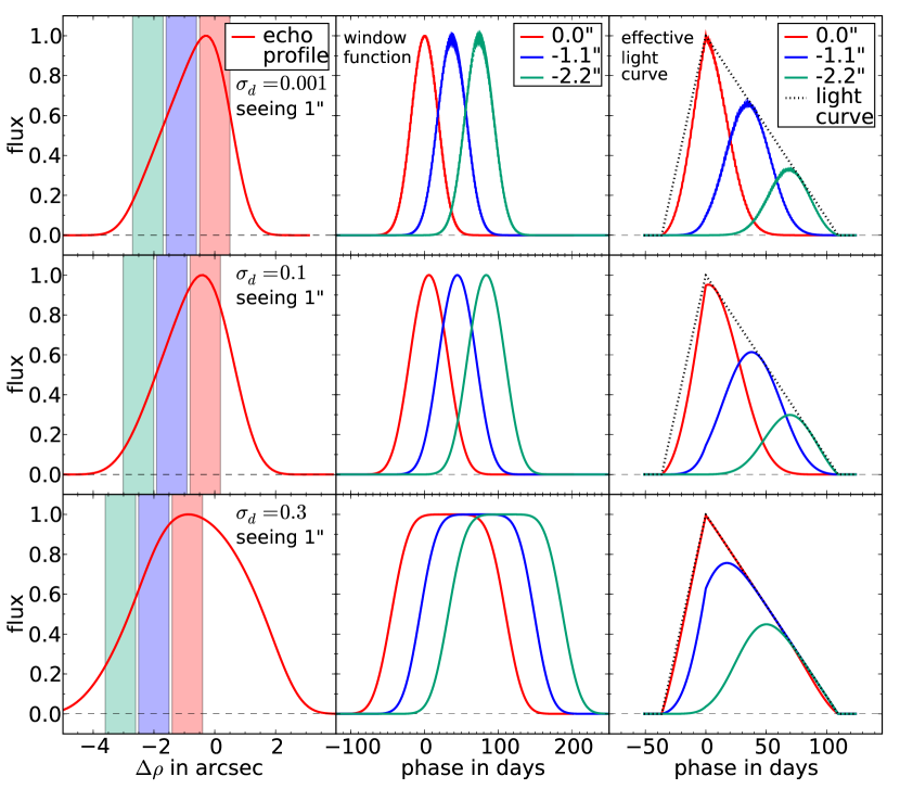
Figure 7.— Same as Figure 6 but in $1\hbox{${}^{\prime\prime}$}$ seeing.

Figure 8 illustrates the application of this model to a “real world” set of conditions. We define a coordinate system ($\Delta\rho,u$), where as before $\Delta\rho=\rho-\rho_{0}$, and $u$ is orthogonal to the $\rho$-axis through $\Delta\rho=0.0$ in the plane of the sky. For a dust filament that is locally planar and perpendicular to the ($\rho,z$) plane, i.e. parallel to $u$, the LE is aligned with the $u$ axis. However, if it is tilted with respect to $u$ by an angle of $\delta_{1}$, then the LE will also be tilted by the same angle (see gray shaded area in illustration). We consider a slit (red box in Figure 8) that is misaligned with the LE by an angle $\delta_{2}$, and also offset along the $\rho$ axis by $\Delta s$.

In this situation, we can recover the proper LE window functions. To do so, we can split the slit into multiple subslits, (in this example, we show this with the horizontal dotted lines). For each of these subslits, we determine the LE profile, calculate the offset of the subslit to the LE using $\delta_{2}$ and $\Delta s$ as described in Appendix C, and determine the window function for each subslit. The total window function for the full slit is then the flux-weighted average of the subslit window functions.

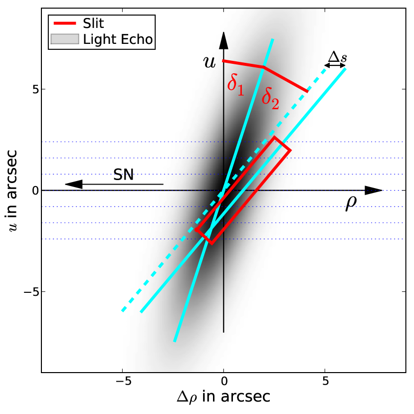
Figure 8.— Toy model of a LE and spectroscopic slit configuration where the slit is misaligned both in angle and offset relative to the LE. The LE is indicated with the shaded area. We define a coordinate system ($\rho,u$) in the plane of the sky centered at the LE, where the $\rho$ axis is in the direction to the source event, and $u$ is perpendicular to $\rho$, with the positive direction along positive position angle of LE-SNR. The LE is along the $u$ axis if the dust filament is perpendicular to the ($\rho,z$) plane. In this example he angle $\delta_{1}$ between the LE and the $u$-axis is 18^∘, and the angle $\delta_{2}$ between slit and LE is 22^∘. Six subslits of width $0.8\hbox{${}^{\prime\prime}$}$ are indicated with the blue dotted lines. The offset $\Delta s$ is $1.0\hbox{${}^{\prime\prime}$}$.

4. Cas A Light Echoes

4.1. Observations

As a case study, we investigate LEs discovered in a multi-season campaign beginning in October 2006 on the Mayall 4 m telescope at Kitt Peak National Observatory (Rest et al., 2008b). The MOSAIC imager on the Mayall 4 m telescope, which operates at the f/3.1 prime focus at an effective focal ratio of f/2.9, was used with the Bernstein “$V\!R$” broad filter ($\lambda_{c}=595$ nm, $\delta\lambda=212$ nm; NOAO Code k1040). The imaging data was kernel- and flux-matched, aligned, subtracted, and masked using the SMSN pipeline (Rest et al., 2005a; Garg et al., 2007; Miknaitis et al., 2007). We investigate the three Cas A SN light echoes LE2116, LE2523, and LE3923, for which we presented spectra in Rest et al. (2010). Figure 9 shows the difference images and the slit position for these three LEs, and Table 1 lists the positions, lengths, and position angles for each slit. LE2116 was previously reported by Rest et al. (2008b), whereas LE2521 and LE3923 were discovered on 2009 September 14 and 16, respectively. For the analysis of LE2116, we use images from 2009 September 14, while we use the discovery images for LE2521 and LE3923.

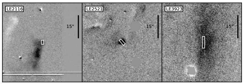
Figure 9.— Difference image cutouts for LE2116, LE2521, and LE3923 from left to right, respectively. For all image stamps north is up and east is left. Excess flux in the first and second epoch is white and black, respectively. The position and size of the spectroscopic slit is indicated by the white rectangle.

Table 1

		RA	Dec	PA SNR-LE	Seeing	Width	Length	PA
LE	Telescope	(J2000)	(J2000)	(∘)	(′′)	(′′)	(′′)	(∘)
LE2116	Keck	23:02:27.10	+56:54:23.4	237.83	0.81	1.5	2.69	00.0
LE2521	Keck	23:12:03.86	+59:34:59.3	299.11	0.79	1.5	4.32	41.0
LE3923	Keck	00:21:04.97	+61:15:37.3	065.08	0.89	1.5	7.72	00.0

4.2. Cas A Light Echo Template Spectra

There are several LEs associated with the Cas A SN. Here we examine three LEs for which we have spectra. Their profiles are shown in Figure 10. To fit the LE profiles, we numerically solve the model defined by Equation A14 for the observed data. To do this, we assume that the explosion occurred in the year $1681\pm 19$ (Fesen et al., 2006), determine the scattering dust coordinates $\rho_{0}$ and $z_{0}$ by using Equation A1 with the measured angular separation between the LE and the SNR, and we determine the dust inclination from the apparent motion of the LEs (this process is defined in Appendix E and described in more detail by Rest et al., in prep.). The remaining free model parameters are the LE profile peak height and position and the dust filament width, which has physical implications. For the three LEs presented above, we display their best fit model profiles in Figure 10.

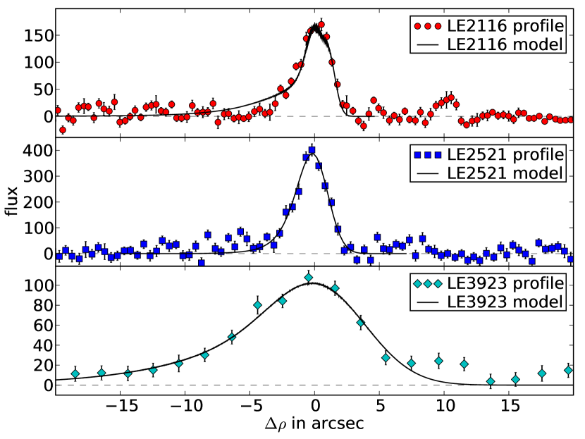
Figure 10.— LE profiles for LE2116, LE2521, and LE3923 from top to bottom, respectively. The model fit is indicated with the black lines.

To numerically fit the model parameters, we determine the best fitting profile by calculating the reduced $\chi^{2}$ for a 3-dimensional grid of the three fit parameters. For each parameter, we marginalize over the other parameters to obtain the best-fitting value. The initial step sizes of the parameter grid are often too large for a proper marginalization. To ensure a proper determination of the parameters, we iterate this process three times adjusting the grid spacing, guided by the fitted parameters and their uncertainties from the previous iteration. In all but the lowest signal-to-noise ratio cases, the probability density functions have a well-behaved Gaussian shape. Figure 11 shows as examples the marginal probability density functions (PDFs) for the peak position and dust width of the LE2521 LE profile at $u=0.5\hbox{${}^{\prime\prime}$}$.

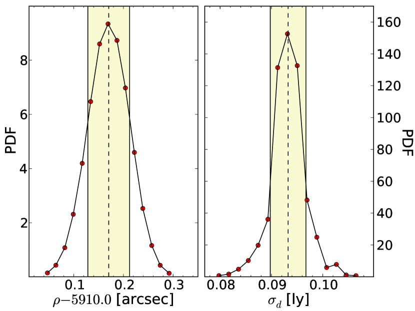
Figure 11.— Probability density functions (PDFs) for the peak position (left) and dust width (right) of LE2521 at $u=0.5\hbox{${}^{\prime\prime}$}$. The most likely value is indicated with a dashed line, and the yellow shaded region indicates the 1-$\sigma$ interval.

Table 2 shows the input and fitted parameters of these three LE profiles. These profiles are for subslits with $u=0.5\hbox{${}^{\prime\prime}$}$, i.e., close to the center of the spectroscopic slit. The definition of the ($\rho,u$) coordinate system and how it relates to the LE and the subslits is explained in detail in Section 3.4, Appendix C and Figure 8. LE2116 and LE2521 have profiles with a similar width. The profile of LE3923, however, has a significantly larger width. Note that the model fits the data very well.

Table 2

	Image	Seeing	$\alpha$	$\delta_{1}$	$\delta_{2}$	$\Delta\rho_{\rm offset}$	$\rho_{0}$	$z_{0}$	$\sigma_{d}$	$S\!B$	$\sigma_{s,{\rm eff}}$
LE	UT Date	(′′)	(∘)	(∘)	(∘)	(′′)	(ly)	(ly)	(ly)	(mag)	(′′)
LE2116	20090914	0.97	09(5)	-07.80	$-39.97$	$-0.42$	0627.9561(18)	0437.11	0.031(10)	22.82(02)	1.77
LE2521	20090914	1.13	54(5)	$-10.98$	0$-0.91$	$-0.01$	0317.9613(23)	00$-9.89$	0.093(04)	21.83(02)	1.53
LE3923	20090916	1.65	07(5)	-10.44	$-35.36$	$-0.35$	1203.8904(76)	2045.38	0.614(53)	23.35(04)	1.65

Note. — All the values are for the subslits with $u=0.5$.

Figure 12 shows the fitted LE peak position $\rho_{0}$, dust width $\sigma_{d}$, and peak surface brightness $S\!B$ for all subslits of each of the three LEs. Panels A–C show $\rho_{0}$ for the three LEs, with the spectroscopic slit overplotted (black solid lines). The dashed line indicates a straight line fit to the subslits that are within the spectroscopic slit. Even though there is some structure in the $\rho_{0}$ versus $u$ relation, locally the LE position can be approximated very well with a straight line. Panel D shows the dust width $\sigma_{d}$. The dust width of LE3923 is nearly constant over $20\hbox{${}^{\prime\prime}$}$ and is an order of magnitude larger than the dust width of the other two LEs. The dust width for LE2116 decreases and then increases over only $\sim\!\!$ $2\hbox{${}^{\prime\prime}$}$. The width decreases to $\sigma_{d}=0.03$ ly for $u\geq 0.5$, making this portion of the LE2116 filament the thinnest yet observed. We discuss potential scientific opportunities for a LE with such a thin dust width in Section 6.3. Panel E shows the surface brightness. LE2521 has a surface brightness brighter than 21 mag/arcsec^-2 and is the brightest Cas A LE yet reported. However, it is spatially small. On the other hand, LE3923 is relatively faint, but its large size makes spectroscopy productive.

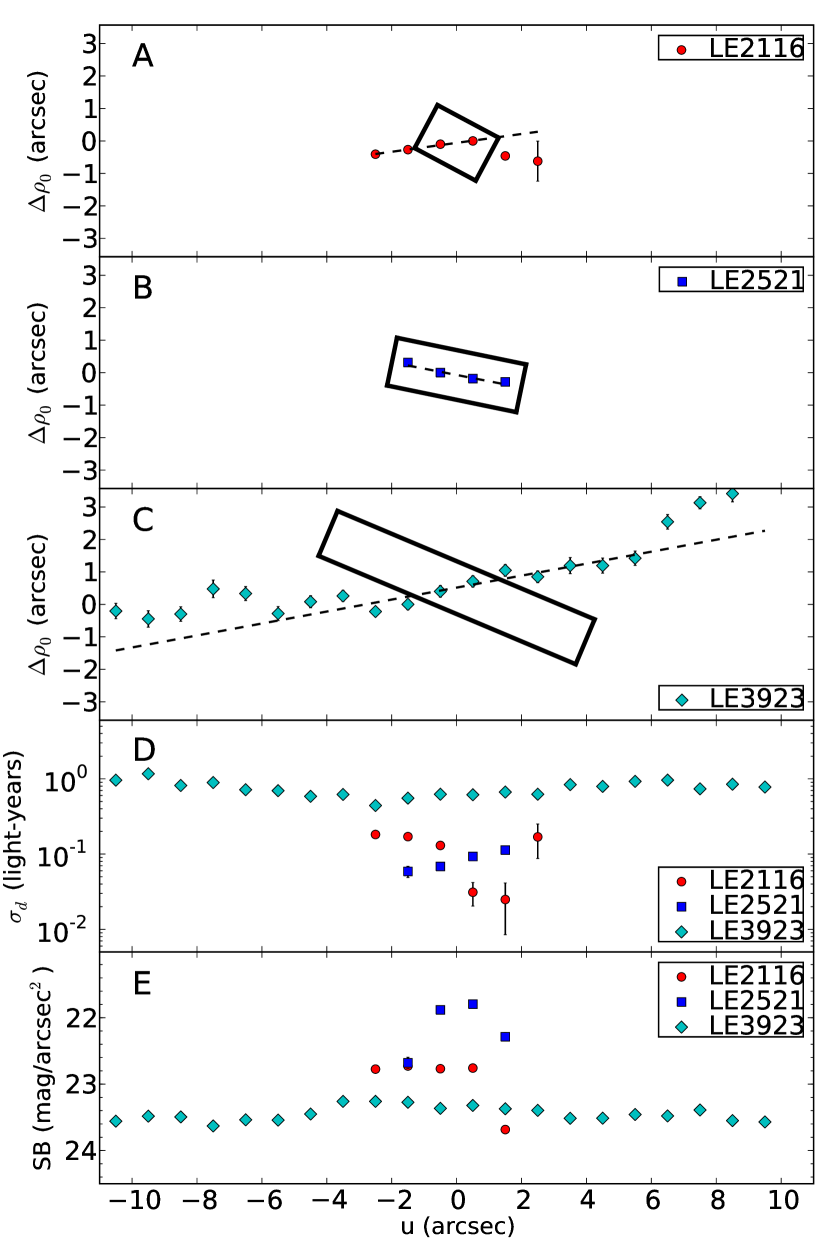
Figure 12.— Panel A, B, and C show the positions of the LE profile peaks for the different subslits for LE2116, LE2521, and LE3923, respectively. $\Delta\rho_{0}(u)$ is defined as $\rho_{0}(u)-\rho_{0}(0)$, and $u$ is orthogonal to the $\rho$-axis through $\rho_{0}(0)$. Red, blue, and cyan symbols indicate LE2116, LE2521, and LE3923, respectively. Panel D shows the fitted dust widths, $\sigma_{d}$, and Panel E shows the surface brightnesses.

For the spectra presented by Rest et al. (2010), the profile fits had not been completed when slit masks were designed. As a result, the alignment between the LEs and the slit were not optimal. In particular, there is a large misalignment in angle for LE3923; however, that LE has a large profile (${\rm FWHM}\approx 10\hbox{${}^{\prime\prime}$}$; see bottom panel of Figure 10) and therefore an offset at the 1–2^′′ scale does not decrease the total amount of flux by a significant amount. However, it does affect the observed spectra since the window function and effective light curves strongly depend on these offsets.

For each LE, we calculate the window function by fitting the observed LE profile with the numerical model as described above. The spectroscopic slit is applied to the fitted LE profile using Equations B1–B4 as described in Appendix B. It is important to note that now the seeing from the spectroscopic observation is used instead of the seeing from the image used to determine the LE profile. For each slit, the weighted average of all subslits is calculated using Equations C1 – C4 in Appendix C.

The top panel of Figure 13 shows the window functions for the three LEs for which we have spectra. The middle panel shows the SN 1993J light curve and the effective light curves for each LE (using the LE profiles and assuming that their light curves are the same as SN 1993J).

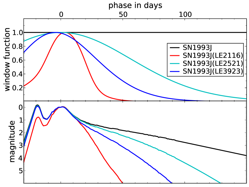
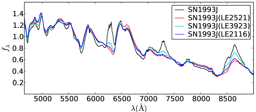
Figure 13.— Top: window function for the different LEs. Middle: effective light curves of SN 1993J for the LEs. The unmodified light curve of SN 1993J is shown in black. Bottom: integrated SN 1993J spectra, where the integration is weighted by the respective effective light curve. Red, cyan, and blue curves represent LE2116, LE2521, and LE3923, respectively. The black spectrum is weighted by the original, unmodified SN 1993J light curve. The differences in the spectra are mainly due to the strong [O I] $\lambda\lambda 6300$, 6363, [Ca II] $\lambda\lambda 7291$, 7324, and Ca II NIR triplet features in the late-phase spectra.

Even though LE2521 and LE2116 have comparable dust widths, the dust inclination for LE2521 is significantly larger, resulting in a wider window function than LE2116. This also causes the projected SN light-curve shape to be “squashed.” LE3923 has a similar inclination to that of LE2116, but its scattering dust is thicker, also leading to a wider window function. Note that the three window functions, and therefore also the effective light curves (see middle panel in Figure 13), have significantly dropped off after 100 days past maximum. However, the decline time of SN is significantly longer, and consequently the contribution of spectra with phases $\geq 100$ days is cut off - a fact illustrated in the bottom panel of Figure 13, which shows the integrated spectra for SN 1993J. The late type spectra of SN IIb like SN 1993J are dominated by [O I] $\lambda\lambda 6300$, 6363, [Ca II] $\lambda\lambda 7291$, 7324, and the Ca II NIR triplet. Note that the black spectrum, which is weighted by the original, un-modified light curve, is much stronger at the position of these lines compared to the other spectra, which are integrated using the effective light curves. We conclude that a perfectly symmetrical SN observed at different position angles might be erroneously interpreted as asymmetrical if scattering dust properties, seeing, and slit width are not taken into account.

4.3. Light Echo Spectra: Systematics

We have shown in Section 3 with simulated light curves and dust filaments how the LE spectra are influenced by the dust properties and observing conditions, and in Section 4.2 we have applied this to the real-world example of the Cas A LEs. In this section, we investigate how changing these properties impacts the LE spectra. We start with the fit to the Cas A LE profiles of LE2521 described in Section 4.2, and create a window function, effective light curve, and LE spectrum using using the spectroscopic and photometric library of SN 1993J as a template. We then vary dust width, dust inclination, and seeing while keeping all other parameters fixed.

Figure 14 shows the effective light curves (left panels) and integrated SN 1993J spectra (right panels). In the top panel, we vary the dust width, $\sigma_{d}$. We find that, consistent with the simulations in Section 3, the nebular [O I] and [Ca II] lines in the integrated spectra have a strong dependence on the dust width. For $\sigma_{d}\lesssim 0.1$ ly, the [O I] and [Ca II] emission lines are weak, whereas for larger values the integrated spectrum quickly approaches the limit of the integrated spectrum without any window function applied with strong [O I] and [Ca II] emission lines. We find similar results for the dust inclination: the difference between the integrated spectra is small and the [O I] and [Ca II] lines are weak for $\alpha\lesssim 60$^∘, but then rapidly approaches the integrated spectrum without any window function applied for $\alpha$ close to 90^∘. We find that the seeing (bottom panel) only has a very strong impact on the observed LE spectrum if the dust width is very small as discussed in Section 6.2 and 6.3.

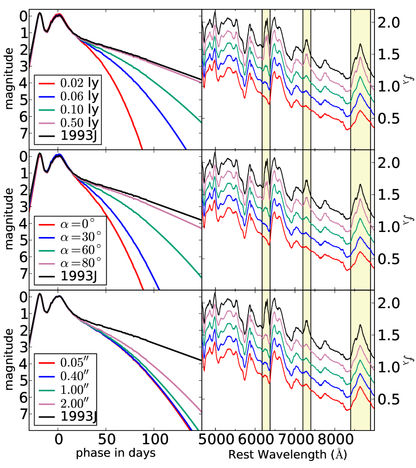
Figure 14.— Effective light curves and integrated SN 1993J spectra varying the dust width, $\sigma_{d}$ (top row), the dust inclination, $\alpha$ (middle row), and the seeing (bottom row) for LE2521. For a given row, only one parameter varies, with the other parameters are set by the fit described above and shown in Figure 10. The black line indicates the original SN 1993J light curve and the corresponding integrated spectra.

We also investigate how uncertainties in the dust inclination impact the derived integrated spectra template. To do this, we fixed the dust inclination from 0^∘ to 80^∘for LE2521, and fit the LE profile. Figure 15 shows the fitted dust width, $\sigma_{d}$, with respect to the input dust inclination, $\alpha$. Three examples of the fitted LE profiles are shown in the top panel of Figure 16. The bottom panels show the corresponding effective light curves (left) and integrated spectrum (right).

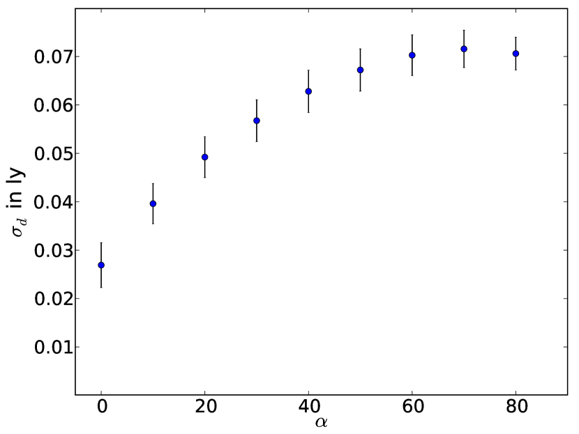
Figure 15.— Fitted dust width, $\sigma_{d}$, for the LE2521 LE profile for different input dust inclination, $\alpha$.

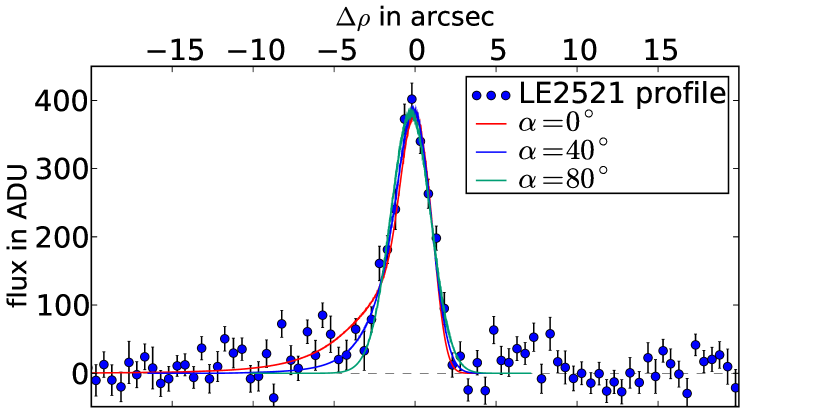
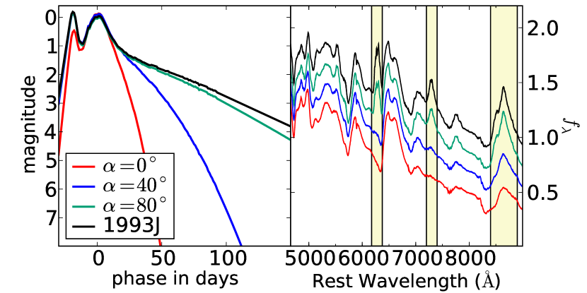
Figure 16.— Top: LE2521 profile and model fits for varying inclination angles, $\alpha$. Bottom: Effective light curves (left) and the corresponding integrated spectra (right). The black line indicates the original SN 1993J light curve and the corresponding integrated spectra.

Note that while the LE profile fit is very good in all cases, the effective light curves are different, and thus the integrated spectra differ significantly in [O I] and [Ca II] line strengths. The reason for these differences is the degeneracy between the dust inclination and the dust width. For decreasing dust inclination (i.e., the dust inclination gets closer to the tangential of the LE paraboloid), the projected light curve is “stretched.” This effect can be nullified by decreasing the dust width, resulting in a similar fit to the LE profile with significantly different parameters (see Figure 15).

For inclinations close to 90^∘, the LE profile is dominated by the dust profile and not by the projected light-curve profile. Such a situation manifests itself in a LE profile that is symmetrical (see green line in top panel of Figure 16) in contrast to the asymmetrical LE profile shape (see red line in top panel of Figure 16) that still reveals indications of the original light curve. Similarly, the fitted $\sigma_{d}$ is essentially constant for $\alpha\approx 90\hbox{${}^{\circ}$}$.

The tests in this section have shown that an incorrect dust inclination can systematically bias the interpretation of SN properties from LE spectra. We discuss the sources of uncertainty in the determination of the inclination in Appendix E.

5. SN 1987A Light Echoes

5.1. Observations

Beginning in 2001, the SuperMACHO Project microlensing survey employed the CTIO 4 m Blanco telescope with its 8K $\times$ 8K MOSAIC imager (plus its atmospheric dispersion corrector) to monitor the central portion of the LMC every other night for 5 seasons (September through December). The images were taken through our custom “$V\!R$” filter ($\lambda_{c}=625$ nm, $\delta\lambda=220$ nm; NOAO Code c6027). SN 1987A and its LEs are in field sm77, which was observed with exposure times between 150 and 200 seconds. We have continued monitoring this field since the survey ended. The difference imaging reduction process was identical to the KPNO Cas A imaging.

5.2. Profile Modeling

The ring-shaped LEs associated with SN 1987A have previously been studied in great detail, mapping the dust structure surrounding the SN (e.g., Sugerman et al., 2005b). Unlike historical SNe, a complete spectral and photometric history of the SN is available for SN 1987A. This historical database allows an observed LE spectrum to be modeled unambiguously against a spherically symmetric model for the explosion. In addition, the high signal-to-noise ratio of the SN 1987A LEs make them ideal for our tests.

We consider an example LE from SN 1987A corresponding to a unique position angle on the sky. The spectrum associated with this LE was taken using the Gemini Multi-Object Spectrograph (GMOS; Hook et al., 2004) on Gemini-South, using the R400 grating. The spectroscopic slit was $1.0\hbox{${}^{\prime\prime}$}$ wide and $2.16\hbox{${}^{\prime\prime}$}$ long, with the slit tilted to be tangential to the observed LE ring. The upper panel of Figure 17 shows the apparent motion of the LE monitored over more than a year. The motion on the sky is constant on such time scales ($4.09\pm 0.02$ ^′′/year), indicating constant inclination of the dust structure. To determine the angle of inclination, $\alpha$, we translate ($\rho,t$) into $(z,\rho)$ as described in Appendix E, resulting in a dust inclination of $\alpha=30.4\pm 0.8$^∘ (see lower panel of Figure 17).

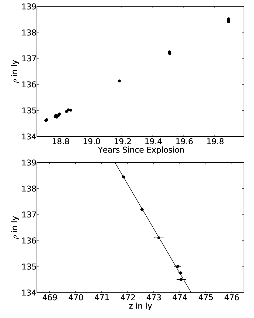
Figure 17.— Top: Apparent motion of a single position angle of the LE system of SN 1987A. The uniform motion of the LE on the sky indicates a unique inclination for the dust structure. The superluminal motion of the LE is $4.09\pm 0.02~{}\hbox{${}^{\prime\prime}$}$/year. Bottom: The above $(\rho,t)$ data is binned when observations are taken within 10 days of each other, and converted to the $(z,\rho)$ plane using equation A1. The resulting fit (solid line) gives an inclination of $\alpha=30.4\pm 0.8$^∘.

A high signal-to-noise ratio difference image is used to model the effect of the dust on the spectroscopic slit. Input parameters are the inclination ($\alpha=30.4$^∘), observed seeing for the image ($1.22\hbox{${}^{\prime\prime}$}$), and delay time since explosion ($ct=19.9$ years). The photometric data of SN 1987A (Hamuy et al., 1988; Suntzeff et al., 1988; Hamuy & Suntzeff, 1990) are used to model the LE profile observed on the sky, with the best-fitting model shown in the left panel of Figure 18. The dust structure model is able to recreate the observed LE profile exceedingly well. The window function and resulting effective light curve associated with the spectroscopic slit (convolved to the seeing at time of spectroscopy) are shown in the middle and right panels of Figure 18, respectively. The average dust width associated with the spectroscopic slit is $\sigma_{d}=4.26\pm 0.06$ ly ($1.31\pm 0.02$ pc). We note that at the inclination and dust widths observed here, the model is less sensitive to uncertainties in $\alpha$. Testing of the model shows that at such inclinations, uncertainties in $\alpha$ on the order of 5^∘ have little impact on the window function and resulting integrated spectrum (see Section 3.2).

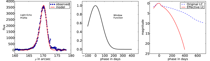
Figure 18.— Left: observed profile for the SN 1987A LE, with the best-fit model profile over-plotted. Middle: resulting window function associated with the $1.0\hbox{${}^{\prime\prime}$}$ wide spectroscopic slit. Right: effective light curve from the model compared with the original light curve of SN 1987A.

The impact of the scattering dust is clear when fitting the model to the observed spectrum. To integrate the spectral history of SN 1987A we take advantage of the extensive spectral database from SAAO and CTIO observations after the explosion (Menzies et al., 1987; Catchpole et al., 1987, 1988; Whitelock et al., 1988; Catchpole et al., 1989; Whitelock et al., 1989; CTIO_87aspec1; CTIO_87aspec2). Figure 19 shows the observed LE spectrum (black), the model spectrum (red), and the full light-curve integrated spectrum (blue dashed). Note that the observed LE spectrum includes strong nebular emission lines that are not associated with the SN. Both the model spectrum and the full light-curve weighted integrated spectrum show a good fit for features blueward of 5500 Å. However, the lower panel of Figure 19 shows that the spectrum redward of 5500 Å, and in particular the H$\alpha$ feature, are best fit by the spectrum corresponding to the best-fit LE profile model. From Figure 18, it is clear that the strength of the H$\alpha$ feature in the integrated spectrum is highly dependent on the window function. At late times, the spectra of SN 1987A are dominated by strong H$\alpha$ emission. The excellent fit to the LE spectrum of SN 1987A validates our method of determining the effective light curve from the LE profile.

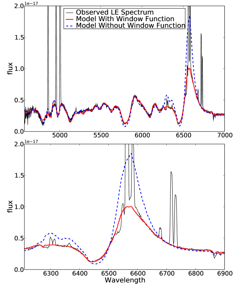
Figure 19.— Top: Observed LE spectrum of SN 1987A (black) with the best-fit model (using the window function from Figure 18) integrated spectrum (red) and the full light-curve weighted integrated spectrum (blue). Bottom: Detail of the spectra near the H$\alpha$ feature. Note that the narrow lines dominating the emission peak of the profile are strong nebular emission lines, and are not associated with the SN. The best-fit model integrated spectrum fits the observed LE spectrum well in this region, while the full light-curve weighted integrated spectrum is a poor fit.

5.3. Impact of Dust Parameters on Observed Spectrum

Similar to the analysis performed in Section 4.3, we vary the three free parameters of our model to determine their impact on the observed LE spectrum for SN 1987A. Figure 20 shows the effective light curves (left column) and integrated SN 1987A spectra (right column). The top, middle, and bottom rows show the model varying the dust width ($\sigma_{d}$), dust inclination ($\alpha$), and seeing, respectively, while holding the other parameters constant. To emphasize the differences in the integrated spectra, the figure focuses on the H$\alpha$ feature. The advantage of the SN 1987A observations over those of Cas A is that there is a complete linking between the LE and the final integrated spectrum via observation, since we have a priori knowledge of the SN creating the observed LE profile.

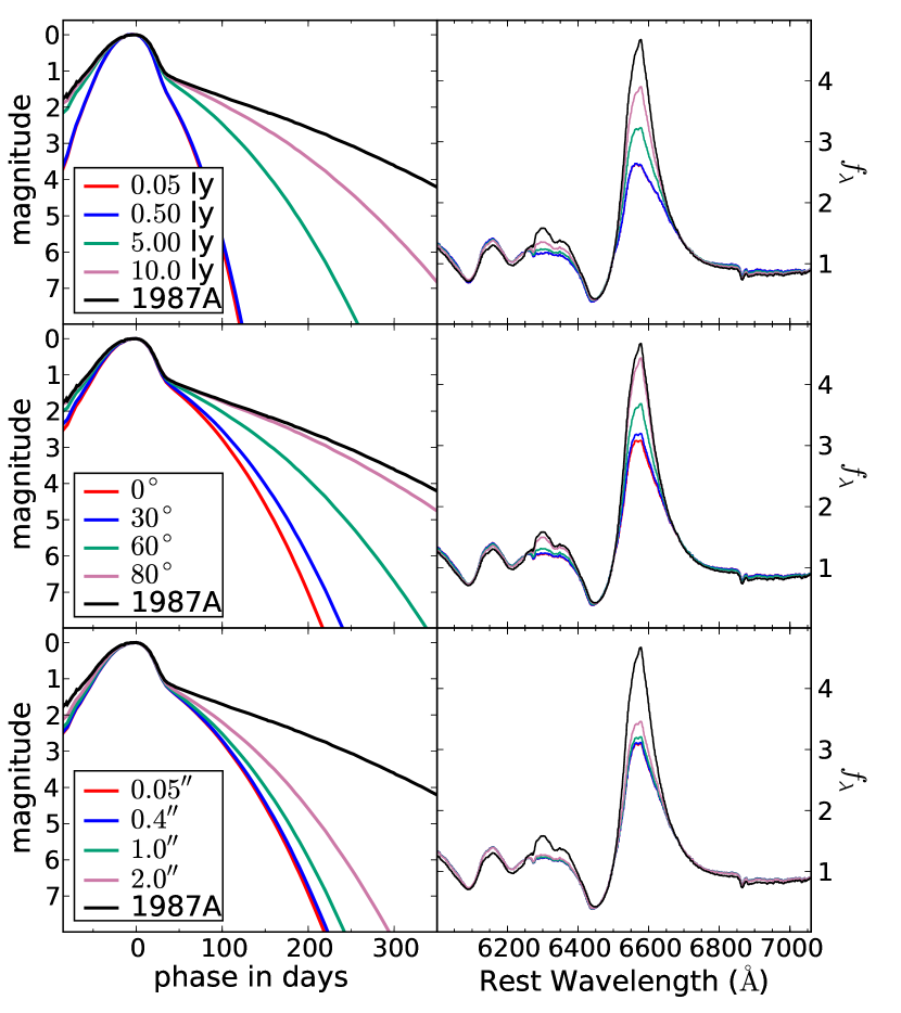
Figure 20.— Effective light curves (left column) and integrated spectra (right column) for SN 1987A, varying the dust width, $\sigma_{d}$ (top row), the dust inclination, $\alpha$ (middle row), and the seeing (bottom row). For a given row, only one parameter varies, with the other parameters are set by the fit described above and shown in Figure  18.

The dependence on the integrated spectra of SN 1987A are similar to that of SN 1993J (see Figure 14), where increasing the dust width, inclination, or seeing all share the result of stretching the weight function closer to the $wf=1$ case, resulting in an effective light curve approaching that of the original SN 1987A light curve. Figure 20 allows us to rank the impact of the dust parameters on the observed LE spectrum. Seeing has the least significance on the spectrum, although we note that poor image quality should still be taken into account. Dust inclination has a large effect, although the sensitivity is small if the dust is close to perpendicular to the observer. The dust width has the greatest impact on the spectrum, which is particularly noteworthy since this quantity has been ignored until now. For SN 1987A, the H$\alpha$ peak height increases by about 20% if the dust thickness is 10 ly instead of 5 ly, indicating a sensitivity that exceeds that of the other parameters.

Figure 20, as well as the SN 1987A spectrum presented in Section 5.2, clearly show the danger in interpreting spectroscopic data from LEs without proper modeling. Any interpretation of LE spectra based on relative line strengths must be accompanied by a careful analysis of the dust properties associated with the LE.

6. Discussion

In the previous sections, we have presented the LE model, the dependency of the model on various parameters, and have applied that model to multiple real-world cases. In this section, we discuss how we can use our new understanding of LEs and the scattering dust to perform additional observations that will provide new insight into historical SNe.

6.1. Verification of Model Parameters And Systematic Biases

The analysis of SN 1987A LEs has the added benefit that the validity of our dust models and their impact on the observed LE profiles and spectra can be tested, since the spectrophotometric evolution of the SN itself has been monitored extensively. We show in Section 5 and in more detail in Sinnott et al. (2011) that the observed LE profile, apparent motion, and spectra can all be brought in excellent accordance with what is predicted using the SN 1987A spectrophotometric library and our dust model locally parameterized as a planar filament with a Gaussian density profile. This shows that at least in the case of SN 1987A, the Gaussian dust model is a good approximation of the true dust profile.

In general, dust structures are filamentary in nature, which is easily visible in its effect on the shapes of LEs, which often show twists and furcations. However, on the few arcsecond scale, most of the shape and profiles of LEs change slowly over months and even years. For example, the dust width, $\sigma_{d}$, for LE3923 and LE2521 is nearly constant over 20^′′ (see second panel from the bottom in Figure 12) and smoothly increasing, respectively. In order to account for small changes in the dust parameters, we split the slit into 1^′′ sections and fit the dust parameters separately for each of these sections.

If there are significant deviations from the Gaussian dust density model (e.g., if there is substructure in the density on small scales), the window function can potentially be biased, which in turn, can cause spectral differences that would be interpreted as intrinsic to the SN. We can test and guard against these systematic biases: LEs often come in “groups”; i.e., there are often several distinct LEs separated by tens of arcseconds for LEs of Galactic SNe. The scattering dust filaments likely belong to the same dust structure, but are tens of light years apart. Therefore any substructure in these filaments is uncorrelated. For LEs of the same source event only tens or hundred of arcseconds apart, the physical properties of the source event are the same. An upper limit on the systematic bias can be set by the differences in the observed spectra which are not accounted for by the differences in fitted dust parameters. In all data obtained by our team, we have not found any evidence that there are significant biases in our analysis due to substructure in the dust or deviation from the dust model. This is particularly important for the two novel methods that we describe in the next two sections.

If LEs from two different SNe are reflected off the same dust, then the dust thickness measured from our method should be the same for both sets of LEs. Such a scenario is a direct test of the model fits. Fortunately, this situation occurs for LEs from Cas A and Tycho, and a comparison of the derived values will be presented in a future work. Since this situation was discovered in a relatively small and low filling factor survey, it is reasonable to expect other such regions of the sky exist where dust is at the intersection of two historical SN LE ellipsoids.

6.2. Temporally Resolving Light Echo Spectra

One of the most exciting opportunities LEs present is to use them to temporally resolve the SN spectrum: If a slit is aligned perpendicular to a LE profile instead of parallel, different parts of the slit probe different epochs of the SN light curve.

As an example, we imagine a SN LE where the SN is a carbon copy of SN 1993J, the dust filament is at $z=400$ ly with an inclination of 0^∘ and a width of 0.02 ly. With a Hubble Space Telescope-like (HST) PSF FWHM of $0.05\hbox{${}^{\prime\prime}$}$, the projected light curve would have minimal distortion. If a spectrum is taken with the slit perpendicular to the LE arc (i.e., parallel to the line from the LE to the SNR) with $0.05\hbox{${}^{\prime\prime}$}$ seeing, then the spatially resolved spectrum (i.e., moving along the axis perpendicular to the wavelength direction) corresponds to a temporally resolved spectrum. The left panel of Figure 21 shows the effective light curves for this situation if spectra are extracted from $1\hbox{${}^{\prime\prime}$}$ long parts of the slit. The offset from the peak of the LE are $1.0\hbox{${}^{\prime\prime}$}$, $0.0\hbox{${}^{\prime\prime}$}$, and $-1.0\hbox{${}^{\prime\prime}$}$ along the $\rho$-axis. The right panel shows the corresponding integrated spectra. The three spectra show clear differences, in particular the spectra with $\Delta\rho_{\rm offset}=1.0$ is very blue since it is dominated by the first peak of the light curve.

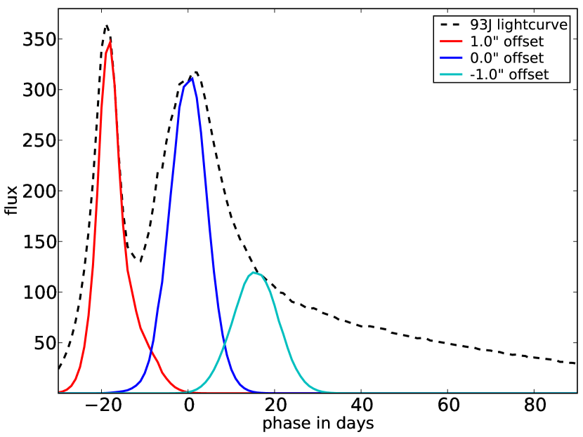
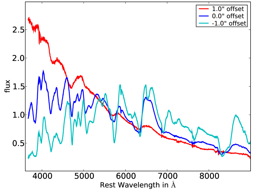
Figure 21.— Left: Effective light curves for LE2116 with a $1\hbox{${}^{\prime\prime}$}$ slit and offsets, $\Delta\rho_{\rm offset}$, of $-1.0\hbox{${}^{\prime\prime}$}$, $0.0\hbox{${}^{\prime\prime}$}$, and $1.0\hbox{${}^{\prime\prime}$}$ shown in red, blue, and cyan, respectively. Right: Integrated spectra corresponding to the effective light curves in the left panel.

Aligning the slit perpendicular to the LE can significantly reduce the amount of light within the slit, and therefore, this method is best applied to the brightest LEs. To maximize the temporal resolution of the LE spectra, the LE should have the following properties:

1. The dust filament is very thin— on the order of 0.01 ly.

2. The inclination is close to the LE ellipsoid tangential. This “stretches” the projected light curve along the $\rho$-axis.

3. The LE is bright.

4. The PSF of the spectroscopic observation is small.

Even though there are no known Galactic LEs that fulfill all of these criteria, we note that the existing surveys are far from complete. Additionally, even in non-ideal conditions, some temporal information could be obtained. The ability to temporally resolve the SN spectra will allow us to follow the evolution of the explosion, specifically measure velocity gradients of spectral features, and potentially probing the abundances of elements in the ejecta.

6.3. Constraining Supernova Light-Curve Shapes

Under similar circumstances needed to temporally resolve the LE spectra (see Section 6.2), we will also be able to spatially resolve the temporal characteristics of the source event light curve. The most important requirements are that the dust width has to be thin, the inclination close to the LE ellipsoid tangential, and the PSF needs to be significantly smaller than the width of the LE profile. Note that in contrast to temporally resolving the LE spectra, constraining the LE shape can be done with LEs that have a significantly lower signal-to-noise ratio.

Unfortunately, there is a degeneracy between the dust width and the light curve parameters (e.g., peak width and height; peak ratio if double-peaked) which can be broken if different areas of the LE have different dust widths. Since the light curve must be the same for all LEs in a given direction, any difference in the shape must be from the dust. If this degeneracy cannot be broken, LEs can still provide interesting constraints. First, the light curve can only be broadened by the dust, so any profile will provide some constraint on the light-curve shape. Additionally, by comparing the profile to known SN light curves, the properties of the SN can be further constrained.

The light-curve shape of a SN can give important insights into the nature of the SN explosion. SNe Ia, for example, show a clear relationship between the width of their light curves and their intrinsic brightness (e.g., Phillips, 1993). Another example is if the shock break-out of a core-collapse SN is resolved in the light curve, which would provide a measurement (or strict constraints) on the radius of the progenitor star. We will discuss this in more detail in the following paragraphs.

After the gravitational collapse of the core of a massive star, the core bounces, sending a shock wave out through the outer layers of the star, exploding the star (Woosley & Weaver, 1986). When the shock wave reaches the surface of the star, a flash (at optical wavelengths, it has a thermal spectrum) is generated that decays over hours to days (Colgate, 1974; Klein & Chevalier, 1978). This has been seen for SNe IIP (Gezari et al., 2008; Schawinski et al., 2008), but was best observed recently with SN Ib 2008D (Soderberg et al., 2008; Modjaz et al., 2009). As the stellar envelope cools, the optical emission fades away. This subsequent fading was first detected in SN 1987A (e.g., Woosley et al., 1987; Hamuy et al., 1988), which had a shock break-out cooling phase that was unusually long. This cooling phase has been detected for a handful of other SNe, notably SN 1993J (e.g., Richmond et al., 1994), a SN IIb similar to Cas A.

The duration, luminosity, and SED of the shock break-out phase depends on a handful of parameters such as the presence of a stellar wind and the ejecta mass (Matzner & McKee, 1999), but is most dependent on the progenitor radius (Calzavara & Matzner, 2004). The peak brightness of the subsequent fading is dependent on the ejecta mass, kinetic energy, and progenitor radius, while the timescale for the fading is proportional to both the radius of the photosphere and its temperature (Waxman et al., 2007). One caveat is that interaction of the shock with shells of material outside the star can produce prompt emission similar to a shock breakout.

The disadvantage of using LEs to observe the shock break-out is that if the resolution of the image is poor or the dust thickness is too large, it is impossible to distinguish between a shock break-out, subsequent fading, and normal radioactive-decay powered SN light curve, and a somewhat broader radioactive-decay powered SN light curve. For Cas A, where we might expect to see a shock break-out, we are unable to separate the light curve into multiple components in ground-based images with moderate seeing ($<1$^′′). However, as shown in Figure 22, if the dust thickness is sufficiently small, we should detect a luminous shock break-out with the resolution of HST, if it exists. This will allow us to constrain the radius of the progenitor and its mass loss history, linking the physical properties of a star with its SNR.

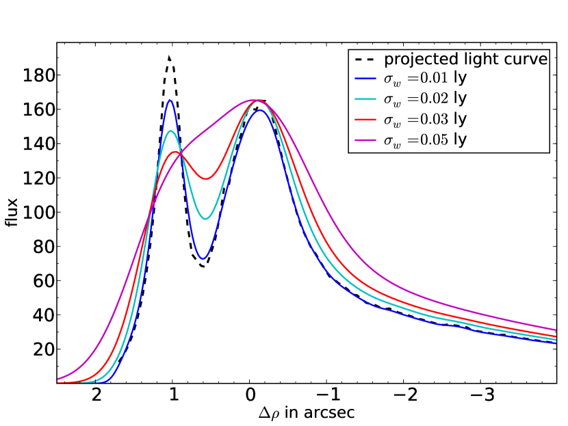
Figure 22.— Simulated LE profiles of SN 1993J assuming different scattering dust widths. The scattering dust filament for the simulations is at $z=400$ ly with an inclination of 0^∘, and the PSF FWHM is $0.05\hbox{${}^{\prime\prime}$}$, similar to what can be expected from space-based imaging. The black dashed line is the projected SN 1993J light curve.

7. Conclusions

In recent years, LEs of SNe have offered the rare opportunity to spectroscopically classify the SN type hundreds of years after the light of the explosion first reached the Earth (e.g., Rest et al., 2008a). Recently, we have obtained the first spectroscopic observations of a historical SN from different lines of sight using LEs (Rest et al., 2010). These observations provide the unique opportunity to examine a SN from different directions, with the light for each LE coming from slightly different hemispheres of the SN. In this paper, we have demonstrated that to properly separate differences in the observed LE spectra caused by intrinsic asymmetries in the SN from those caused by scattering dust, seeing, and spectroscopic slit position, it is necessary to properly model the latter.

Throughout this paper, we have shown how to both determine the properties of the scattering dust and their influence, as well as that of the PSF and spectroscopic slit position, on the observed LE spectra. We found that the dust width and inclination are the dominant factors, especially when the dust filament is thin. These two factors can be degenerate with respect to the LE profile shape; therefore, it is essential to determine the dust filament inclination independently using the LE proper motion from images taken at two (or more) epochs. The slit width and its misalignment with the major axis of the LE are is also a significant factor. The image PSF smears out the observed LE and thus also impacts the observed LE spectrum. Taking all of these factors into account, we found that the observed LE spectrum is not the light-curve weighted integration of the spectra at all epochs, but rather the integration of the spectra weighted by an effective light curve. This effective light curve is the original light curve convolved with a window function, and it is different for every LE location. In general, the most significant difference between the effective light curves and the original light curve was that later epochs tend to be truncated in the effective light curves.

We used fits to the LE profiles of Cas A and SN 1987A to test the consistency and veracity of our model. We fit the model to the observed LE profiles, where the three free parameters were the LE profile peak height, LE position, and – physically most important – the dust filament width. The model reproduced the observed LE profiles very well, and we found that it was possible to determine all factors influencing the observed LE spectrum a priori just from images, without using the observed spectrum.

We constructed window functions and effective light curves for the Cas A LEs using SN 1993J as a template. We found a much better match of the SN 1993J spectra template to the observed Cas A LE spectrum if we used the effective light curve instead of the real light curve for weighting. The most significant difference was in the late-phase emission lines [O I] $\lambda\lambda 6300$, 6363, [Ca II] $\lambda\lambda 7291$, 7324, and the Ca II NIR triplet, consistent with our expectation from the model. Although we do not have access to the Krause et al. (2008) images, we find that their Cas A spectrum is consistent with an integrated spectrum weighted with a light curve truncated at 80 days. Our expectation is that the majority of differences between the Cas A LE spectrum and the full light-curve weighted SN 1993J spectrum are due to scattering dust properties.

We also constructed a window function and effective light curve for a SN 1987A LE which constitutes a special test case since the light curve and spectral data of the SN are available. With this data, we constructed a LE spectrum from the original SN and compared it to the observed LE spectrum. We found that the constructed LE spectrum correctly predicted the line strength of the H$\alpha$ line, while a simple integration weighted by the light curve was a poor fit.

We presented several additional investigations that can be attempted with LEs in the near future. Two of these studies, temporally resolved spectra and spatially resolved light curves, require thin dust filaments. Until now, the assumption of thick scattering dust prevented such studies.

Appendix A Light Echo Profiles

The LE equation (Couderc, 1939),

$$z=\frac{\rho^{2}}{2ct}-\frac{ct}{2},$$ (A1)

relates the depth coordinate, $z$, the LE-SN distance projected along the line-of-sight, to the LE distance $\rho$ perpendicular to the line of sight, and the time $t$ since the initial (undelayed) arrival of SN photons. Then the distance $r$ from the scattering dust to the source event is $r^{2}=\rho^{2}+z^{2}$, and $\rho$ is

$$\rho=(D-z)\sin\gamma,$$ (A2)

where $D$ is the distance from the observer to the source event, and $\gamma$ is the angular separation between the source event and the scattering dust, which yields the three-dimensional position of the dust associated with the arclet.

Tylenda (2004) elegantly derives the apparent expansion of a LE ring caused by a thin plane-parallel sheet of dust. In a very similar manner, we derive how the dust filament inclination influences the observed LE profile. Because of the symmetry around the $z$-axis, we define our coordinate system so that the dust sheet is normal in the ($\rho,z$) plane. This allows us to do all our calculations in the two-dimensional ($\rho,z$) space. We define the dust sheet as

$$z=z_{d}-a\rho,$$ (A3)

where $a=\tan\alpha$. We define $\alpha$ as the angle of the dust sheet with respect to the $\rho$ axis, where positive angles go from the positive $\rho$ axis towards the negative $z$ axis. The dust sheet intersects with the $z$ axis at $z=z_{d}$. The two intersections of the dust sheet with the reflection paraboloid defined in Equation A1 are then

$$\rho_{\pm}(t,z_{d},a) =-act\pm\xi,\mbox{ where}$$ (A4)

$$\xi =\sqrt{\left(1+a^{2}\right)\left(ct\right)^{2}+2z_{0}ct}.$$ (A5)

Now consider a LE caused by a source event with a peak at $t_{0}$ at an angular separation $\gamma$ from the source. Assuming a distance $D$ to the source event, we can then calculate the position of the scattering dust $(\rho_{0},z_{0})$ using Equation A1 and A2. The dust sheet defined in Equation A3 goes through ($\rho_{0},z_{0}$) if

$$z_{d}=z_{0}+a\rho_{0}.$$ (A6)

There are two special dust inclinations. We denote the inclination angle of the dust sheet tangential and orthogonal to the LE ellipse as $\alpha_{\parallel}$ and $\alpha_{\perp}$, respectively. Then the slopes of the dust sheets are $a_{\parallel}=\tan{\alpha_{\parallel}}$, and $a_{\perp}=\tan{\alpha_{\perp}}$, and we can calculate them as

$$a_{\parallel} =-\left(1+\frac{2z_{0}}{ct}\right)^{1/2}=-\frac{\rho_{0}}{ct};$$ (A7)

$$a_{\perp} =-a_{\parallel}^{-1}=\left(1+\frac{2z_{0}}{ct}\right)^{-1/2}=\frac{ct}{\rho_{0}}.$$ (A8)

The intersection of the dust sheet with the LE ellipsoid is then at

$$\rho_{0}=\begin{cases}0&\mbox{for }\alpha=90\hbox{${}^{\circ}$}\\ \rho_{+}&\mbox{for }a>a_{\parallel}\\ \rho_{-}&\mbox{for }a<a_{\parallel}\end{cases}.$$ (A9)

Now consider a dust sheet with a finite width defined by a density $D(\Delta r)$, and a light curve $f_{\rm source}(\Delta t)$, where $\Delta r$ is the distance orthogonal to the dust sheet, and $\Delta t=t-t_{0}$ (see Section D for a more detailed description of the dust model $D(\Delta r)$). The flux from the source event at time $t$ is reflected by the part of the dust sheet at a distance $\Delta r$ to the center of the dust sheet, and makes a relative contribution to the LE signal of

$$f_{\rm LE}=D(\Delta r)f_{\rm source}(\Delta t)$$ (A10)

at the position

$$\rho_{\rm LE}=\begin{cases}\rho_{+}(t_{0}+\Delta t,z_{d}+\Delta r/\cos{\alpha},a)&\mbox{if }\rho_{0}=\rho_{+}\\ \rho_{-}(t_{0}+\Delta t,z_{d}+\Delta r/\cos{\alpha},a)&\mbox{if }\rho_{0}=\rho_{-}\end{cases}.$$ (A11)

The reason for choosing $+$ and $-$ is based on the choice made for $\rho_{0}$. For all practical purposes, $\Delta r$ and $\Delta t$ are small, and therefore the sign should be the same. Exceptions are $\alpha\approx 0.0$ and $a\approx a_{\parallel}$. We define

$$\Delta\rho=\rho_{\rm LE}-\rho_{0}.$$ (A12)

By examining the relative contribution for all values of $\Delta r$ and $\Delta t$ and using Equation A10 – A12, we can calculate a cumulative grid of fluxes, $F^{\prime}_{\rm LE}(\Delta t,\Delta\rho)$.

The model must now account for seeing. We describe the data PSF as a Gaussian with a FWHM of $x$ arcsec and Gaussian width of $\sigma_{\rm PSF}=x/(2\sqrt{2\ln(2)})\approx x/2.35$. Then the cumulative grid of fluxes convolved with the seeing is

$$F_{\rm LE}(\Delta t,\Delta\rho)=\sum_{\Delta\rho^{\prime}}F^{\prime}_{\rm LE}(\Delta t,\Delta\rho^{\prime})\frac{1}{\sqrt{2\pi\sigma_{\rm PSF}^{2}}}\exp{\left(\frac{(\Delta\rho-\Delta\rho^{\prime})^{2}}{2\sigma_{\rm PSF}^{2}}\right)}.$$ (A13)

Integrating over $\Delta t$ returns the LE flux profile with respect to $\rho$:

$$P_{\rm LE}(\Delta\rho)=\int F_{\rm LE}(\Delta t,\Delta\rho)\mathrm{d}t.$$ (A14)

Appendix B Dependence of the Light Echo Spectrum on Light Echo Profile

We now examine the LE flux for a spectroscopic observation. Consider a slit positioned at $\rho_{s}$ with a effective width of $\sigma_{s,{\rm eff}}$. The reason that this is the effective slit width and its relation to the real, physical slit width $\sigma_{s}$ is explained below in Appendix C. We define the offset between the slit and the LE measured parallel to the $\rho$ axis as $\Delta\rho_{\rm offset}=\rho_{s}-\rho_{0}$. The slit then subtends from

$$\Delta\rho_{\min} =\Delta\rho_{\rm offset}-\sigma_{s,{\rm eff}}/2\mbox{ to}$$ (B1)

$$\Delta\rho_{\max} =\Delta\rho_{\rm offset}+\sigma_{s,{\rm eff}}/2.$$ (B2)

We can then calculate the relative contribution, $H(\Delta t)$, of the source event at time $\Delta t$ to the spectra with

$$H(\Delta t)=\int_{\Delta\rho_{\min}}^{\Delta\rho_{\max}}F_{\rm LE}(\Delta t,\Delta\rho)\mathrm{d}\Delta\rho.$$ (B3)

$H(\Delta t)$ is also the effective light curve. We define the window function $w(\Delta t)$ as the fractional difference between the effective light curve and the real light curve,

$$w(\Delta t)=f_{\rm source}(\Delta t)/H(\Delta t).$$ (B4)

The observed LE spectrum $S_{\rm LE}(\lambda)$ is then

$$S_{\rm LE}(\lambda)=\int S(\lambda,\Delta t)H(\Delta t)\mathrm{d}\Delta t,$$ (B5)

where $S(\lambda,\Delta t)$ is the spectrum of the source event at the given phase $\Delta t$.

Appendix C Dependence of the Light Echo Spectrum on Slit Position

The position and inclination of the slit with respect to the LE has a major impact on the observed spectrum. We illustrate this in Figure 8. We define a coordinate system ($\rho,u$), where $u$ is orthogonal to $\rho$ through $\Delta\rho=0.0$ in the plane of the sky. For a dust filament that is locally planar and perpendicular to the ($\rho,z$) plane (i.e., parallel to $u$), the LE is aligned with the $u$ axis. However, if it is tilted with respect to $u$ by an angle of $\delta_{1}$, then the LE will also be tilted by the same angle (see gray shaded area in Figure 8).

Now consider a slit (red box in Figure 8) that is misaligned with the LE by an angle $\delta_{2}$, and also offset along the $\rho$ axis by $\Delta s$. We split the slit into subslits, indicated with the dotted blue lines in Figure 8. For each of these subslits, we determine the LE profile in Figure 8. The offset $\Delta\rho_{{\rm offset},i}$ of the subslit $i$ centered at $u_{i}$ to the LE is

$$\Delta\rho_{{\rm offset},i}=u_{i}\sin(\delta_{2})+\Delta s,$$ (C1)

where $\delta_{2}$ is the angle between the slit and the LE, and $\Delta s$ is the offset of the center of the slit to the LE (see Figure 8). The effective slit width $\sigma_{s,{\rm eff}}$ depends on the physical slit width $\sigma_{s}$ and is

$$\sigma_{s,{\rm eff}}=\sigma_{s}/\cos(\delta_{2}).$$ (C2)

The effective light curve $H_{i}$ and window function $w_{i}$ for each subslit $i$ can be calculated plugging $\Delta\rho_{{\rm offset},i}$ into Equation B1 and B2. The total window function $w_{\rm slit}$ for the full slit is then the weighted average of the subslit window functions, where the weight is the flux $f_{w}$ that falls into the subslit is

$$f_{w,i} =\int_{\Delta\rho_{\min}}^{\Delta\rho_{\max}}P_{\rm LE}(\Delta\rho)\mathrm{d}\Delta\rho\mbox{ with}$$ (C3)

$$w_{\rm slit} =\frac{\sum_{i}w_{i}f_{w,i}^{-2}}{\sum_{i}f_{w,i}^{-2}}.$$ (C4)

The integrated spectrum can then be calculated by using $w_{\rm slit}$ in Equations B4 and B5.

Appendix D Dust Model

For simplicity in our simulations, we choose a box-car dust density profile $D(\Delta r)$. A more realistic density profile is a Gaussian, and therefore when fitting observed LE profiles we use a profile

$$D(\Delta r)=\frac{c}{\sqrt{2\pi\sigma_{d}^{2}}}\exp{\left(\frac{\Delta r^{2}}{2\sigma_{d}^{2}}\right)},$$ (D1)

where $\sigma_{d}$ is the width of the Gaussian, and $c$ is a normalization factor. Note that the physical dust density profile width $\sigma_{d,{\rm phys}}$ is different from the nominal fitted $\sigma_{d}$ if $\delta_{1}\neq 0$. They are related through

$$\sigma_{d,{\rm phys}}=\sigma_{d}\cos(\delta_{1}).$$ (D2)

Appendix E Dust Filament Inclination

We refer the reader to a more thorough and detailed discussion about the apparent motion and its dependence on the dust filament inclination by Rest et al. (in prep.). However, we present an initial treatment of the process here. We define the dust filament inclination $\alpha$ as

$$\alpha=\tan^{-1}\left(-\frac{z(t_{2})-z(t_{1})}{\rho(t_{2})-\rho(t_{1})}\right)$$ (E1)

with $t_{2}>t_{1}$, and with $z$ calculated from Equation A1 for a measured $\rho$ and given $t$. Note that a dust filament in the plane of the sky has $\alpha=0\hbox{${}^{\circ}$}$, and dust filaments tilted away from the observer have positive $\alpha$. If more than two epochs are available, fitting a straight line through ($\rho,z$) increases the accuracy of $\alpha$.

There are several sources that can introduce errors into the measurement of the dust inclination, specifically:

• Poisson uncertainty in the apparent motion of the LE, especially for the fainter LEs

• A small number of epochs

• Intrinsic differences in the filament inclination with $\rho$

The first two mainly increase the Poisson noise in the inclination. The last one, however, is the most significant one since it can introduce systematic uncertainties. If the dust filament has additional substructure, such as twisted dust on small scales, then the inclination of the scattering dust changes on small scales and a correct constraint on the dust inclination at the time of spectroscopy can only be done if there are several epochs close to the time of the spectroscopy.

References

- Badenes et al. (2008) Badenes, C., Hughes, J. P., Cassam-Chenaï, G., & Bravo, E. 2008, ApJ, 680, 1149
- Bond et al. (1990) Bond, H. E., Gilmozzi, R., Meakes, M. G., & Panagia, N. 1990, ApJ, 354, L49
- Bond et al. (2003) Bond, H. E., et al. 2003, Nature, 422, 405
- Calzavara & Matzner (2004) Calzavara, A. J., & Matzner, C. D. 2004, MNRAS, 351, 694
- Cappellaro et al. (2001) Cappellaro, E., et al. 2001, ApJ, 549, L215
- Catchpole et al. (1987) Catchpole, R. M., et al. 1987, MNRAS, 229, 15P
- Catchpole et al. (1988) ——. 1988, MNRAS, 231, 75P
- Catchpole et al. (1989) ——. 1989, MNRAS, 237, 55P
- Colgate (1974) Colgate, S. A. 1974, ApJ, 187, 333
- Couderc (1939) Couderc, P. 1939, Annales d’Astrophysique, 2, 271
- Crotts (1988) Crotts, A. 1988, IAU Circ., 4561, 4
- Dwek & Arendt (2008) Dwek, E., & Arendt, R. G. 2008, ApJ, 685, 976
- Fesen et al. (2006) Fesen, R. A., et al. 2006, ApJ, 645, 283
- Filippenko (1997) Filippenko, A. V. 1997, ARA&A, 35, 309
- Filippenko et al. (1992) Filippenko, A. V., et al. 1992, ApJ, 384, L15
- Garavini et al. (2004) Garavini, G., et al. 2004, AJ, 128, 387
- Garg et al. (2007) Garg, A., et al. 2007, AJ, 133, 403
- Gezari et al. (2008) Gezari, S., et al. 2008, ApJ, 683, L131
- Hamuy & Suntzeff (1990) Hamuy, M., & Suntzeff, N. B. 1990, AJ, 99, 1146
- Hamuy et al. (1988) Hamuy, M., Suntzeff, N. B., Gonzalez, R., & Martin, G. 1988, AJ, 95, 63
- Hook et al. (2004) Hook, I. M., Jørgensen, I., Allington-Smith, J. R., Davies, R. L., Metcalfe, N., Murowinski, R. G., & Crampton, D. 2004, PASP, 116, 425
- Hughes et al. (1995) Hughes, J. P., et al. 1995, ApJ, 444, L81
- Kapteyn (1902) Kapteyn, J. C. 1902, Astronomische Nachrichten, 157, 201
- Klein & Chevalier (1978) Klein, R. I., & Chevalier, R. A. 1978, ApJ, 223, L109
- Krause et al. (2008) Krause, O., Birkmann, S. M., Usuda, T., Hattori, T., Goto, M., Rieke, G. H., & Misselt, K. A. 2008, Science, 320, 1195
- Krause et al. (2005) Krause, O., et al. 2005, Science, 308, 1604
- Liu et al. (2003) Liu, J.-F., Bregman, J. N., & Seitzer, P. 2003, ApJ, 582, 919
- Matzner & McKee (1999) Matzner, C. D., & McKee, C. F. 1999, ApJ, 510, 379
- Meikle et al. (2006) Meikle, W. P. S., et al. 2006, ApJ, 649, 332
- Menzies et al. (1987) Menzies, J. W., et al. 1987, MNRAS, 227, 39P
- Miknaitis et al. (2007) Miknaitis, G., et al. 2007, ApJ, 666
- Modjaz et al. (2009) Modjaz, M., et al. 2009, ApJ, 702, 226
- Newman & Rest (2006) Newman, A. B., & Rest, A. 2006, PASP, 118, 1484
- Phillips (1993) Phillips, M. M. 1993, ApJ, 413, L105
- Phillips et al. (1992) Phillips, M. M., Wells, L. A., Suntzeff, N. B., Hamuy, M., Leibundgut, B., Kirshner, R. P., & Foltz, C. B. 1992, AJ, 103, 1632
- Quinn et al. (2006) Quinn, J. L., Garnavich, P. M., Li, W., Panagia, N., Riess, A., Schmidt, B. P., & Della Valle, M. 2006, ApJ, 652, 512
- Rest et al. (2007) Rest, A., et al. 2007, in Bulletin of the American Astronomical Society, Vol. 38, Bulletin of the American Astronomical Society, 935–+
- Rest et al. (2010) Rest, A., et al. 2010, ArXiv e-prints, 1003.5660
- Rest et al. (2008a) ——. 2008a, ApJ, 680, 1137
- Rest et al. (2005a) ——. 2005a, ApJ, 634, 1103
- Rest et al. (2005b) ——. 2005b, Nature, 438, 1132
- Rest et al. (2008b) ——. 2008b, ApJ, 681, L81
- Richmond et al. (1994) Richmond, M. W., Treffers, R. R., Filippenko, A. V., Paik, Y., Leibundgut, B., Schulman, E., & Cox, C. V. 1994, AJ, 107, 1022
- Ritchey (1901a) Ritchey, G. W. 1901a, ApJ, 14, 293
- Ritchey (1901b) ——. 1901b, ApJ, 14, 167
- Ritchey (1902) ——. 1902, ApJ, 15, 129
- Schawinski et al. (2008) Schawinski, K., et al. 2008, Science, 321, 223
- Schmidt et al. (1994) Schmidt, B. P., Kirshner, R. P., Leibundgut, B., Wells, L. A., Porter, A. C., Ruiz-Lapuente, P., Challis, P., & Filippenko, A. V. 1994, ApJ, 434, L19
- Sinnott et al. (2011) Sinnott, B., et al. 2011, in prep.
- Soderberg et al. (2008) Soderberg, A. M., et al. 2008, Nature, 453, 469
- Sparks et al. (1999) Sparks, W. B., Macchetto, F., Panagia, N., Boffi, F. R., Branch, D., Hazen, M. L., & della Valle, M. 1999, ApJ, 523, 585
- Sugerman (2005) Sugerman, B. E. K. 2005, ApJ, 632, L17
- Sugerman & Crotts (2002) Sugerman, B. E. K., & Crotts, A. P. S. 2002, ApJ, 581, L97
- Sugerman et al. (2005a) Sugerman, B. E. K., Crotts, A. P. S., Kunkel, W. E., Heathcote, S. R., & Lawrence, S. S. 2005a, ApJ, 627, 888
- Sugerman et al. (2005b) ——. 2005b, ApJS, 159, 60
- Suntzeff et al. (1988) Suntzeff, N. B., Heathcote, S., Weller, W. G., Caldwell, N., & Huchra, J. P. 1988, Nature, 334, 135
- Swope (1940) Swope, H. H. 1940, Harvard College Observatory Bulletin, 913, 11
- Tylenda (2004) Tylenda, R. 2004, A&A, 414, 223
- van den Bergh (1965) van den Bergh, S. 1965, PASP, 77, 269
- van den Bergh (1966) ——. 1966, PASP, 78, 74
- Van Dyk et al. (2006) Van Dyk, S. D., Li, W., & Filippenko, A. V. 2006, PASP, 118, 351
- Wang et al. (2008) Wang, X., Li, W., Filippenko, A. V., Foley, R. J., Smith, N., & Wang, L. 2008, ApJ, 677, 1060
- Waxman et al. (2007) Waxman, E., Mészáros, P., & Campana, S. 2007, ApJ, 667, 351
- Welch (2007) Welch, D. L. 2007, ApJ, 669, 525
- Whitelock et al. (1989) Whitelock, P. A., et al. 1989, MNRAS, 240, 7P
- Whitelock et al. (1988) ——. 1988, MNRAS, 234, 5P
- Woosley et al. (1987) Woosley, S. E., Pinto, P. A., Martin, P. G., & Weaver, T. A. 1987, ApJ, 318, 664
- Woosley & Weaver (1986) Woosley, S. E., & Weaver, T. A. 1986, ARA&A, 24, 205
- Xu et al. (1995) Xu, J., Crotts, A. P. S., & Kunkel, W. E. 1995, ApJ, 451, 806
- Zwicky (1940) Zwicky, F. 1940, Reviews of Modern Physics, 12, 66