Empirical Comparison of Algorithms for
Network Community Detection

Abstract

Detecting clusters or communities in large real-world graphs such as large social or information networks is a problem of considerable interest. In practice, one typically chooses an objective function that captures the intuition of a network cluster as set of nodes with better internal connectivity than external connectivity, and then one applies approximation algorithms or heuristics to extract sets of nodes that are related to the objective function and that “look like” good communities for the application of interest.

In this paper, we explore a range of network community detection methods in order to compare them and to understand their relative performance and the systematic biases in the clusters they identify. We evaluate several common objective functions that are used to formalize the notion of a network community, and we examine several different classes of approximation algorithms that aim to optimize such objective functions. In addition, rather than simply fixing an objective and asking for an approximation to the best cluster of any size, we consider a size-resolved version of the optimization problem. Considering community quality as a function of its size provides a much finer lens with which to examine community detection algorithms, since objective functions and approximation algorithms often have non-obvious size-dependent behavior.

Categories and Subject Descriptors: H.2.8 Database Management: Database applications – Data mining

General Terms: Measurement; Experimentation.

Keywords: Community structure; Graph partitioning; Conductance; Spectral methods; Flow-based methods.

1 Introduction

Detecting clusters or communities in real-world graphs such as large social networks, web graphs, and biological networks is a problem of considerable practical interest that has received a great deal of attention [16, 17, 13, 8, 19]. A “network community” (also sometimes referred to as a module or cluster) is typically thought of as a group of nodes with more and/or better interactions amongst its members than between its members and the remainder of the network [30, 16].

To extract such sets of nodes one typically chooses an objective function that captures the above intuition of a community as a set of nodes with better internal connectivity than external connectivity. Then, since the objective is typically NP-hard to optimize exactly [24, 4, 31], one employs heuristics [16, 20, 9] or approximation algorithms [25, 33, 2] to find sets of nodes that approximately optimize the objective function and that can be understood or interpreted as “real” communities. Alternatively, one might define communities operationally to be the output of a community detection procedure, hoping they bear some relationship to the intuition as to what it means for a set of nodes to be a good community [16, 29]. Once extracted, such clusters of nodes are often interpreted as organizational units in social networks, functional units in biochemical networks, ecological niches in food web networks, or scientific disciplines in citation and collaboration networks [16, 30].

In applications, it is important to note that heuristic approaches to and approximation algorithms for community detection often find clusters that are systematically “biased,” in the sense that they return sets of nodes with properties that might be substantially different than the set of nodes that achieves the global optimum of the chosen objective. For example, many spectral-based methods tend to find compact clusters at the expense that they are not so well separated from the rest of the network; while other methods tend to find better-separated clusters that may internally be “less nice.” Moreover, certain methods tend to perform particularly well or particularly poorly on certain kinds of graphs, e.g., low-dimensional manifolds or expanders. Thus, drawing on this experience, it is of interest to compare these algorithms on large real-world networks that have many complex structural features such as sparsity, heavy-tailed degree distributions, small diameters, etc. Moreover, depending on the particular application and the properties of the network being analyzed, one might prefer to identify specific types of clusters. Understanding structural properties of clusters identified by various algorithmic methods and various objective functions can guide in selecting the most appropriate graph clustering method in the context of a given network and target application.

In this paper, we explore a range of different community detection methods in order to elucidate these issues and to understand better the performance and biases of various network community detection algorithms on different kinds of networks. To do so, we consider a set of more than 40 networks; 12 common objective functions that are used to formalize the concept of community quality; and 8 different classes of approximation algorithms to find network communities. One should note that we are not primarily interested in finding the “best” community detection method or the most “realistic” formalization of a network community. Instead, we aim to understand the structural properties of clusters identified by various methods, and then depending on the particular application one could choose the most suitable clustering method.

We describe several classes of empirical evaluations of methods for network community detection to demonstrate the artifactual properties and systematic biases of various community detection objective functions and approximation algorithms. We also discuss several meta-issues related to community detection algorithms in very large graphs, including whether or not existing algorithms are sufficiently powerful to recover interesting communities and whether or not meaningful communities exist at all. Also in contrast to previous attempts to evaluate community detection algorithms and/or objective functions, we consider a size-resolved version of the typical optimization problem. That is, rather than simply fixing an objective and asking for an approximation to the best cluster of any size or some fixed partitioning, we ask for an approximation to the best cluster for every possible size. This provides a much finer lens with which to examine community detection algorithms, since objective functions and approximation algorithms often have non-obvious size-dependent behavior.

The rest of the paper is organized as follows. Section 2 gives the background and surveys the rich related work in the area of network community detection. Then, in Section 3.1, we compare structural properties of clusters extracted by two clustering methods based on two completely different computational paradigms—a spectral-based graph partitioning method Local Spectral and a flow-based partitioning algorithm Metis+MQI; and in Section 3.2, we extend the analyses by considering related heuristic-based clustering algorithms that in practice perform very well. Section 4 then focuses on 11 different objective functions that attempt to capture the notion of a community as a set of nodes with better intra- than inter-connectivity. To understand the performance of various community detection algorithms at different size scales we compute theoretical lower bounds on the conductance community-quality score in Section 5. We conclude in Section 6 with some general observations.

2 Related Work and Background

Here we survey related work and summarize our previous work, with an emphasis on technical issues that motivate this paper.

2.1 Related work

A great deal of work has been devoted to finding communities in large networks, and much of this has been devoted to formalizing the intuition that a community is a set of nodes that has more and/or better links between its members than with the remainder of the network. Very relevant to our work is that of Kannan, Vempala, and Vetta [18], who analyze spectral algorithms and describe a community concept in terms of a bicriterion depending on the conductance of the communities and the relative weight of between-community edges. Flake, Tarjan, and Tsioutsiouliklis [11] introduce a similar bicriterion that is based on network flow ideas, and Flake et al. [10] defined a community as a set of nodes that has more edges pointing inside the community than to the rest of the network. Similar edge-counting ideas were used by Radicchi et al. [30] to define and apply the notions of a strong community and a weak community.

Within the “complex networks” community, Girvan and Newman [16] proposed an algorithm that used “betweenness centrality” to find community boundaries. Following this, Newman and Girvan [29] introduced modularity as an a posteriori measure of the overall quality of a graph partition. Modularity measures internal (and not external) connectivity, but it does so with reference to a randomized null model. Modularity has been very influential in recent community detection literature, and one can use spectral techniques to approximate it [34, 28]. However, Guimerà, Sales-Pardo, and Amaral [17] and Fortunato and Barthélemy [13] showed that random graphs have high-modularity subsets and that there exists a size scale below which modularity cannot identify communities.

Finally, we should note several other lines of related work. First, the Local Spectral Algorithm of Andersen, Chung, and Lang [2] was used by Andersen and Lang [3] to find (in a scalable manner) medium-sized communities in very large social graphs. Second, other recent work has also focused on developing local and/or near-linear time heuristics for community detection include [7]. Third, there also exists work which views communities from a somewhat different perspective. For recent reviews of the large body of work in this area, see [14, 31, 12, 21].

2.2 Background and motivation

Figure 1: NCP plot (middle) of a small network (left). NCP of LiveJournal network computed using two different methods.

We model each network by an undirected graph, in which nodes represent entities and edges represent interactions between pairs of entities. We perform the evaluation of community detection algorithms in a large corpus of over $100$ social and information networks. The networks we studied range in size from tens of nodes and scores of edges up to millions of nodes and tens of millions of edges; and they were drawn from a wide range of domains, including large social networks, citation networks, collaboration networks, web graphs, communication networks, citation networks, internet networks, affiliation networks, and product co-purchasing networks. In the present work we focus on a subset of these. In particular, we consider a bipartite authors-to-papers network of DBLP (AuthToPap-DBLP), Enron email network (email-enron), a co-authorship network of Arxiv Astro physics papers (CoAuth-astro-ph), and a social network of Epinions.com (Epinions). See [1] for further information and properties of these networks.

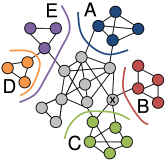
Even though we consider various notions of community score we will primarily work with conductance, which arguably is the simplest notion of cluster quality, as it can be simply thought of as the ratio between the number of edges inside the cluster and the number of edge leaving the cluster [32, 18]. More formally, conductance $\phi(S)$ of a set of nodes $S$ is $\phi(S)=c_{S}/\min(\mbox{Vol}(S),\mbox{Vol}(V\setminus S))$, where $c_{S}$ denotes the size of the edge boundary, $c_{S}=|\{(u,v):u\in S,v\notin S\}|$, and $\mbox{Vol}(S)=\sum_{u\in S}d(u)$, where $d(u)$ is the degree of node $u$. Thus, in particular, more community-like sets of nodes have lower conductance. For example in Figure 1(left), sets $A$ and $B$ have conductance $\phi(A)=\frac{2}{14}>\phi(B)=\frac{1}{11}$, so the set of nodes $B$ is more community-like than the set $A$. Conductance captures a notion of “surface area-to-volume,” and thus it is widely-used to capture quantitatively the gestalt notion of a good network community as a set of nodes that has better internal- than external-connectivity [14, 31].

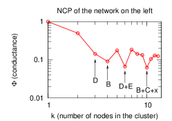
We then generalize the notion of the quality of a single cluster into a size resolved version. Using a particular measure of network community quality $f(S)$, e.g., conductance or one of the other measures described in Section 4, we then define the network community profile (NCP) [27, 26] that characterizes the quality of network communities as a function of their size. For every $k$ between $1$ and half the number of nodes in the network, we define $\Phi(k)=\min_{|S|=k}f(S)$. That is, for every possible community size $k$, $f(k)$ measures the score of the most community-like set of nodes of that size, and the NCP measures $\Phi(k)$ as a function of $k$.

For example, in Figure 1(middle) we use conductance as a measure of cluster quality and for $k=4$, among all sets of $4$-nodes, $B$ has best conductance, and thus $\Phi(4)=\frac{1}{11}$. Similarly, $D$ and $D$+$E$ denote the best conductance sets on $3$ and $6$ nodes, respectively.

Just as the magnitude of the conductance provides information about how community-like is a set of nodes, the shape of the NCP provides insight into how well expressed are network communities as a function of their size. Moreover, the NCP also provides a lens to examine the quality of clusters of various sizes. Thus in the majority of our experiments we will examine and compare different clustering algorithms and objective functions through various notions of the NCP plot and other kinds of structural metrics of clusters and how they depend/scale with the size of the cluster.

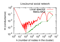
Moreover, the shape of the NCP is also interesting for a very different reason. It gives us a powerful way to quantify and summarize the large-scale community structure of networks. We [27, 26] found that the NCP behaves in a characteristic manner for a range of large social and information networks: when plotted on log-log scales, the NCP tends to have a universal “V” shape (Figure 1(right)). Up to a size scale of about $100$ nodes, the NCP decreases, which means that the best-possible clusters are getting progressively better with the increasing size. The NCP then reaches the minimum at around $k=100$ and then gradually increases again, which means that at larger size scales network communities become less and less community-like. (This should be contrasted with behavior for mesh-like networks, road networks, common network generation models, and small commonly-studied networks, for which the NCP is either flat or downward-sloping [27, 26].) The shape of the NCP can be explained by an onion-like “nested core-periphery” structure, where the network consists of a large core (slightly denser and more expander-like than the full graph, but which itself has a core-periphery structure) and a large number of small very well-connected communities barely connected to the core [27, 26]. In this context, it is important to understand the characteristics of various community detection algorithms in order to make sure that the shape of NCP is a property of the network rather than an artifact of the approximation algorithm or the function that formalizes the notion of a network community.

3 Comparison of algorithms

We compare different clustering algorithms and heuristics. We focus our analyses on two aspects. First, we are interested in the quality of the clusters that various methods are able to find. Basically, we would like to understand how well algorithms perform in terms of optimizing the notion of community quality (conductance in this case). Second, we are interested in quantifying the structural properties of the clusters identified by the algorithms. As we will see, there are fundamental tradeoffs in network community detection—for a given objective function, approximation algorithms are often biased in a sense that they consistently find clusters with particular internal structure.

We break the experiments into two parts. First, we compare two graph partitioning algorithms that are theoretically well understood and are based on two very different approaches: a spectral-based Local Spectral partitioning algorithm, and the flow-based Metis+MQI. Then we consider several heuristic approaches to network community detection that work well in practice.

3.1 Flow and spectral methods

In this section we compare the Local Spectral Partitioning algorithm [2] with the flow-based Metis+MQI algorithm. The latter is a surprisingly effective heuristic method for finding low-conductance cuts, which consists of first using the fast graph bi-partitioning program Metis [20] to split the graph into two equal-sized pieces, and then running MQI, an exact flow-based technique [15, 23] for finding the lowest conductance cut whose small side in contained in one of the two half-graphs chosen by Metis.

Each of those two methods (Local Spectral and Metis+MQI) was run repeatedly with randomization on each of our graphs, to produce a large collection of candidate clusters of various sizes, plus a lower-envelope curve. The lower-envelope curves for the two algorithms were the basis for the plotted NCP’s in the earlier paper [27]. In the current paper the lower-envelope curves for Local Spectral and Metis+MQI are plotted respectively as a red line and a green line in Figure 1(right), and as pairs of black lines in Figure 2(top) and Figures 4 and 7. Note that the Metis+MQI curves are generally lower, indicating that this method is generally better than Local Spectral at the nominal task of finding cuts with low conductance.

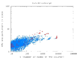
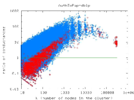
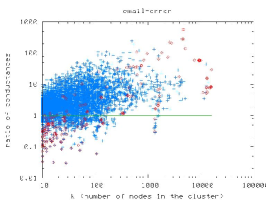
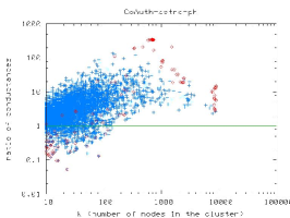
However, as we will demonstrate using the scatter plots of Figure 2, the clusters found by the Local Spectral Method often have other virtues that compensate for their worse conductance scores. As an extreme example, many of the raw Metis+MQI clusters are internally disconnected, which seems like a very bad property for an alleged community. By contrast, the Local Spectral Method always returns connected clusters. Acknowledging that this is a big advantage for Local Spectral, we then modified the collections of raw Metis+MQI clusters by splitting every internally disconnected cluster into its various connected components. Then, in all scatter plots of Figure 2, blue dots represent raw Local Spectral clusters, which are internally connected, while red dots represent broken-up Metis+MQI clusters, which are also internally connected.

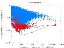
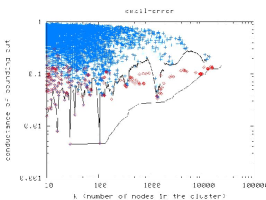
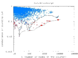
Conductance of connected clusters found by Local Spectral (blue) and Metis+MQI (red)

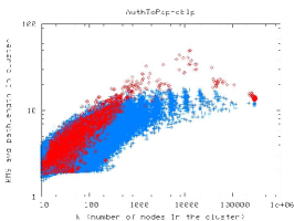
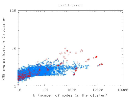
Cluster compactness: average shortest path length

Cluster compactness: external vs. internal conductance

Figure 2: Comparison of Local Spectral (blue) and Metis+MQI (red) on connected clusters. Top: the conductance of the bounding cut. Middle: the average shortest path length in the cluster. Bottom: the ratio of the external conductance to the internal conductance. Generally Metis+MQI yields better cuts while Local Spectral yields clusters that are more compact: they have shorter path lengths and better internal connectivity.

Let us now consider the top row of scatter plots of Figure 2 which compares the conductance scores (as a function of cluster size) of the collections of clusters produced by the two algorithms. The cloud of blue points (Local Spectral clusters) lies generally above the cloud of red points (Metis+MQI clusters), again illustrating that Local Spectral tends to be a weaker method for minimizing conductance score. In more detail, we find that Local Spectral and Metis+MQI tend to identify similar pieces at very small scales, but at slightly larger scales a gap opens up between the red cloud and the blue cloud. At those intermediate size scales, Metis+MQI is finding lower conductance cuts than Local Spectral.

However, the Local Spectral algorithm returns pieces that are internally more compact. This is shown in the middle row of Figure 2 where for each of the (connected) pieces for which we plotted a conductance in the top row, we are now plotting the average shortest path length between random node pairs in that piece. In these plots, we see that in the same size range where Metis+MQI is generating clearly lower conductance connected sets, Local Spectral is generating pieces with clearly shorter internal paths, i.e., smaller diameter sets. In other words, the Local Spectral pieces are more “compact.” This effect is especially pronounced in the DBLP affiliation network, while it also shows up in the Enron email network and the astrophysics collaboration network. Moreover, we made similar observations also for many other datasets (plots not shown).

Finally, in the bottom row of Figure 2 we introduce the topic of internal vs. external cuts, which is something that none of the existing algorithms is explicitly optimizing. These are again scatter plots showing the same set of Local Spectral and Metis+MQI pieces as before, but now the $y$-axis is external conductance divided by internal conductance. External conductance is the quantity that we usually plot, namely the conductance of the cut which separates the cluster from the graph. Internal conductance is the score of a low conductance cut inside the cluster. That is, we take the induced subgraph on the cluster’s nodes and then find best conductance cut inside the cluster.

We then compare the ratios of the conductance of the bounding cut and the internal conductance. Intuitively, good and compact communities should have small ratios, ideally below 1.0, which would mean that those clusters are well separated from the rest of the network and that they are also internally well-connected and hard to cut again. However, the three bottom-row plots of Figure 2 show the ratios. Points above the horizontal line are clusters which are easier to cut internally than they were to be cut from the rest of the network; while points below the line are clusters that were relatively easy to cut from the network and are internally well-connected. Notice that here the distinction between the two methods is less clear. On the one hand, Local Spectral finds clusters that have worse (higher) bounding cut conductance, while such clusters are also internally more compact (have internal cuts of higher conductance). On the other hand, Metis+MQI finds clusters that have better (lower) bounding cut conductance but are also internally easy to cut (have internal cut of lower conductance). Thus when one takes the ratio of the two quantities we observe qualitatively similar behaviors. However, notice that Local Spectral seem to return clusters with higher variance in the ratio of external-to-internal conductance. At small size scales Metis+MQI tends to give clusters of slightly better (lower) ratio, while at larger clusters the advantage goes to Local Spectral. This has interesting consequence for the applications of graph partitioning since (depending on the particular application domain and the sizes and properties of clusters one aims to extract) either Local Spectral or Metis+MQI may be the method of choice.

Also, notice that there are mostly no ratios well below $1.0$, except for very small sizes. This is important, as it seems to hint that large clusters are relatively hard to cut from the network, but are then internally easy to split into multiple sub-clusters. This shows another aspect of our findings: small communities below $\approx 100$ nodes are internally compact and well separated from the remainder of the network, whereas larger clusters are so hard to separate that cutting them from the network is more expensive than cutting them internally. Community-like sets of nodes that are better connected internally than externally don’t seem to exist in large real-world networks, except at very small size scales.

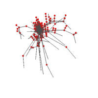
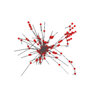
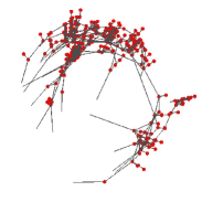
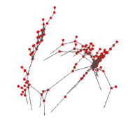
Last, in Figure 3, we further illustrate the differences between spectral and flow-based clusters by drawing some example subgraphs. The two subgraphs shown on the left of Figure 3 were found by Local Spectral, while the two subgraphs shown on the right of Figure 3 were found by Metis+MQI. These two pairs of subgraphs have a qualitatively different appearance: Metis+MQI pieces look longer and stringier than the Local Spectral pieces. All of these subgraphs contain roughly 500 nodes, which is about the size scale where the differences between the algorithms start to show up. In these cases, Local Spectral has grown a cluster out a bit past its natural boundaries (thus the spokes), while Metis+MQI has strung together a couple of different sparsely connected clusters. (We remark that the tendency of Local Spectral to trade off cut quality in favor of piece compactness isn’t just an empirical observation, it is a well understood consequence of the theoretical analysis of spectral partitioning methods.)

Figure 3: Two examples of clusters found by the LocalSpectral algorithm (on the left) and two from the Metis+MQI algorithm (on the right). Note that the Local Spectral clusters are more compact—they are tighter and have smaller diameter since the algorithm has difficulty pushing probability mass down long extended paths—while the Metis+MQI clusters are more sprawling—they have larger diameter and more diverse internal structure, but better conductance scores. In both cases, we have shown communities with ca. $500$ nodes (many of nodes overlap at resolution of this figure).

3.2 Other algorithms

Next we consider various other, mostly heuristic, algorithms and compare their performance in extracting clusters of various sizes. As a point of reference we use results obtained by the Local Spectral and Metis+MQI algorithms.

We have extensively experimented with several variants of the global spectral method, both the usual eigenvector-based embedding on a line, and an SDP-based embedding on a hypersphere, both with the usual hyperplane-sweep rounding method and a flow-based rounding method which includes MQI as the last step. In addition, special post-processing can be done to obtain either connected or disconnected sets.

We also experimented with a practical version of the Leighton-Rao algorithm [24, 25], similar to the implementation described in [22, 23]. These results are especially interesting because the Leighton-Rao algorithm, which is based on multi-commodity flow, provides a completely independent check on Metis, and on spectral methods generally. The Leighton-Rao algorithm has two phases. In the first phase, edge congestions are produced by routing a large number of commodities through the network. We adapted our program to optimize conductance (rather than ordinary ratio cut score) by letting the expected demand between a pair of nodes be proportional to the product of their degrees. In the second phase, a rounding algorithm is used to convert edge congestions into actual cuts. Our method was to sweep over node orderings produced by running Prim’s Minimum Spanning Tree algorithm on the congestion graph, starting from a large number of different initial nodes, using a range of different scales to avoid quadratic run time. We used two variations of the method, one that produces connected sets, and another one that can also produce disconnected sets.

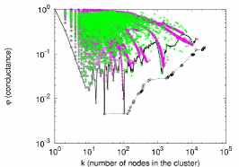
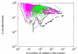
In top row of Figure 4, we show Leighton-Rao curves for three example graphs. Local Spectral and Metis+MQI curves are drawn in black, while the Leighton-Rao curves for connected and possibly disconnected sets are drawn in green and magenta respectively. For small to medium scales, the Leighton-Rao curves for connected sets resemble the Local Spectral curves, while the Leighton-Rao curves for possibly disconnected sets resemble Metis+MQI curves. This further confirms the structure of clusters produced by Local Spectral and Metis+MQI, as discussed in Section 3.1.

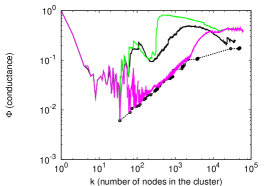
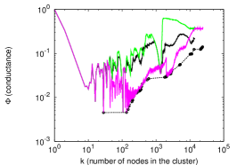
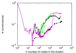
Leighton-Rao: connected clusters (green), disconnected clusters (magenta).

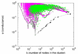
NCP plots obtained by Graclus and Newman’s Dendrogram algorithm.

Figure 4: Comparison of various algorithms on Epinions, Email-Enron, and CA-astro-ph. Top row: NCP plots for connected (green) and disconnected (magenta) pieces from our implementation of the Leighton-Rao algorithm. Bottom row: conductance of cuts found by Graclus and by Newman’s Dendrogram algorithm. Notice the qualitative shape of the NCP plots remains practically unchanged regardless of what particular community detection algorithm we use. Small clusters tend to be connected, while for clusters larger than about 100 nodes connected clusters have around 5 times worse conductance score than disconnected clusters.

At large scales, the Leighton-Rao curves shoot up and become much worse than Local Spectral or Metis+MQI. That Leighton-Rao has troubles finding good big clusters is not surprising because expander graphs are known to be the worst case input for the Leighton-Rao approximation guarantee. Large real networks contain an expander-like core which is necessarily encountered at large scales. We remark that Leighton-Rao does not work poorly at large scales on every kind of graph. (In fact, for large low-dimensional mesh-like graphs, Leighton-Rao is a very cheap and effective method for finding cuts at all scales, while our local spectral method becomes impractically slow at medium to large scales.) This means that based on the structure of the network and sizes of clusters one is interested in different graph partitioning methods should be used. While Leighton-Rao is an appropriate method for mesh-like graphs, it has troubles in the intermingled expander-like core of large networks.

Finally, in addition to the above approximation algorithms-based methods for finding low-conductance cuts, we also experimented with a number of more heuristic approaches that tend to work well in practice. In particular, we compare Graclus [9] and Newman’s modularity optimizing program (we refer to it as Dendrogram) [16]. Graclus attempts to partition a graph into pieces bounded by low-conductance cuts using a kernel $k$-means algorithm. We ran Graclus repeatedly, asking for $2,3,\dots,i,i*\sqrt{2},...$ pieces. Then we measured the size and conductance of all of the resulting pieces. Newman’s Dendrogram algorithm constructs a recursive partitioning of a graph (that is, a dendrogram) from the bottom up by repeatedly deleting the surviving edge with the highest betweenness centrality. A flat partitioning could then be obtained by cutting at the level which gives the highest modularity score, but instead of doing that, we measured the size of conductance of every piece defined by a subtree in the dendrogram.

The bottom row of Figure 4 presents these results. Again our two standard curves are drawn in black. The lower-envelopes of the Graclus or Dendrogram points are roughly similar to those produced by Local Spectral, which means both methods tend to produce rather compact clusters at all size scales. Generally, Graclus tends to produce a variety of clusters of better conductance than Newman’s algorithm. Moreover, notice that in case of Epinions social network and the astrophysics coauthorship network Graclus tends to prefer larger clusters than the Newman’s algorithm. Also, Graclus seems to find clusters of ten or more nodes, while Newmans’s algorithm also extracts very small pieces. In general, clusters produced by either Graclus or Dendrogram are qualitatively similar to those produced by Local Spectral. This means that even though Local Spectral is computationally cheaper and easily scales to very large networks, the quality of identified clusters is comparable to that returned by techniques such as Graclus and Dendrogram that are significantly more expensive on large networks such as those we considered.

4 Comparison of objective functions

In the previous sections, we used conductance since it corresponds most closely to the intuition that a community is a set of nodes that is more and/or better connected internally than externally. In this section, we look at other objective functions that capture this intuition and/or are popular in the community detection literature.

In general there are two criteria of interest when thinking about how good of a cluster is a set of nodes. The first is the number of edges between the members of the cluster, and the second is the number of edges between the members of the cluster and the remainder of the network. We group objective functions into two groups. The first group, that we refer to as Multi-criterion scores, combines both criteria (number of edges inside and the number of edges crossing) into a single objective function; while the second group of objective functions employs only a single of the two criteria (e.g., volume of the cluster or the number of edges cut).

4.1 Multi-criterion scores

Let $G(V,E)$ be an undirected graph with $n=|V|$ nodes and $m=|E|$ edges. Let $S$ be the set of nodes in the cluster, where $n_{S}$ is the number of nodes in $S$, $n_{S}=|S|$; $m_{S}$ the number of edges in $S$, $m_{S}=|\{(u,v):u\in S,v\in S\}|$; and $c_{S}$, the number of edges on the boundary of $S$, $c_{S}=|\{(u,v):u\in S,v\not\in S\}|$; and $d(u)$ is the degree of node $u$.

We consider the following metrics $f(S)$ that capture the notion of a quality of the cluster. Lower value of score $f(S)$ (when $|S|$ is kept constant) signifies a more community-like set of nodes.

• Conductance: $f(S)=\frac{c_{S}}{2m_{S}+c_{S}}$ measures the fraction of total edge volume that points outside the cluster [32, 18].

• Expansion: $f(S)=\frac{c_{S}}{n_{S}}$ measures the number of edges per node that point outside the cluster [30].

• Internal density: $f(S)=1-\frac{m_{S}}{n_{S}(n_{S}-1)/2}$ is the internal edge density of the cluster $S$ [30].

• Cut Ratio: $f(S)=\frac{c_{S}}{n_{S}(n-n_{S})}$ is the fraction of all possible edges leaving the cluster [12].

• Normalized Cut: $f(S)=\frac{c_{S}}{2m_{S}+c_{S}}+\frac{c_{S}}{2(m-m_{S})+c_{S}}$ [32].

• Maximum-ODF (Out Degree Fraction):
  $\max_{u\in S}\frac{|\{(u,v):v\not\in S\}|}{d(u)}$ is the maximum fraction of edges of a node pointing outside the cluster [10].

• Average-ODF: $f(S)=\frac{1}{n_{S}}\sum_{u\in S}\frac{|\{(u,v):v\not\in S\}|}{d(u)}$ is the average fraction of nodes’ edges pointing outside the cluster [10].

• Flake-ODF: $f(S)=\frac{|\{u:u\in S,|\{(u,v):v\in S\}|<d(u)/2\}|}{n_{S}}$ is the fraction of nodes in $S$ that have fewer edges pointing inside than to the outside of the cluster [10].

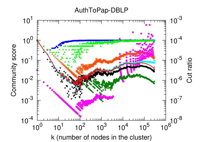
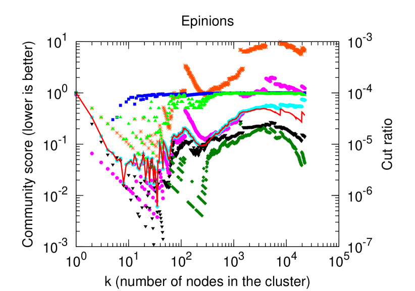
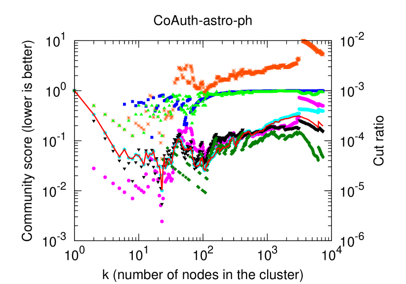
We then generalize the NCP plot: for every cluster size $k$ we find a set of nodes $S$ ($|S|=k$) that optimizes the chosen community score $f(S)$. We then plot community score as a function of $k$. It is not clear how to design an optimization procedure that would, given a cluster size $k$ and the community score function $f(S)$, find the set $S$ that minimizes the function, i.e., is the best community. Operationally, we perform the optimization the following way: we use the Local Spectral method which starts from a seed node and then explores the cluster structure around the seed node; running Local Spectral from each node, we obtain a millions of sets of nodes of various sizes, many of which are overlapping; and then for each such set of nodes, we compute the community score $f(S)$ and find the best cluster of each size.

Figure 5 considers the above eight community scores. Notice that even though scores span different ranges they all experience qualitatively similar behavior, where clusters up to size ca. 100 have progressively better scores, while the clusters above ca. 100 nodes become less community-like as their size increases. This may seem surprising at the first sight, but it should be somewhat expected, as all these objective functions try to capture the same basic intuition—they reward sets of nodes that have many edges internally and few pointing out of the clusters.

There are, however, subtle differences between various scores. For example, even though Flake-ODF follows same general trend as conductance, it reaches the minimum about an order of magnitude later than conductance, normalized cut, cut ratio score or the Average-ODF. On the other hand, Maximum-ODF exhibits the opposite behavior as it clearly prefers smaller clusters and is basically flat for clusters larger than about several hundred nodes. This is interesting as this shows the following trend: if one scores the community by the “worst-case” node using the Out Degree Fraction (i.e., Maximum-ODF) then only small clusters have no outliers and thus give good scores. When one considers the average fraction of node’s edges pointing outside the cluster (Average-ODF) the objective function closely follows the trend of conductance. On the other hand, if one considers the fraction of nodes in the cluster with more of their edges pointing inside than outside the cluster (Flake-ODF), then large clusters are preferred.

Next, focusing on the cut ratio score we notice that it is not very smooth, in the sense that even for large clusters its values seem to fluctuate quite a lot. This indicates that clusters of similar sizes can have very different numbers of edges pointing to the rest of the network. In terms of their internal density, the variations are very small—the internal density reaches the maximum for clusters of sizes around 10 nodes and then quickly raises to 1, which means larger clusters get progressively sparser. For large clusters this is not particularly surprising as the normalization factor increases quadratically with the cluster size. This can be contrasted with the Expansion score that measures the number of edges pointing outside the cluster but normalizes by the number of nodes (not the number of all possible edges).

These experiments suggest that Internal Density and Maximum-ODF are not particularly good measures of community score and the cut ratio score may not be preferred due to high variance. Flake-ODF seems to prefer larger clusters, while conductance, expansion, normalized cut, and Average-ODF all exhibit qualitatively similar behaviors and give best scores to similar clusters.

In addition, we performed an experiment where we extracted clusters based on their conductance score but then also computed the values of other community scores (for these same clusters). This way we did not optimize each community score separately, but rather we optimized conductance and then computed values of other objective functions on these best-conductance pieces. The shape of the plots remained basically unchanged, which suggests that same sets of nodes achieve relatively similar scores regardless of which particular notion of community score is used (conductance, expansion, normalized cut, or Average-ODF). This shows that these four community scores are highly correlated and in practice prefer practically the same clusters.

Figure 5: Various notions of community score as a function of cluster size. All community scores (see main text for descriptions) have qualitatively similar behaviors. They tend to decrease at first, which means clusters get increasingly more community like as their size increases. After that the score tends to degrade (it increases), which means clusters larger than about 100 nodes get progressively less community like.

4.2 Single criterion scores

Next we also consider community scores that consider a single criteria. One such example is Modularity [28], which is one of the most widely used methods to evaluate the quality of a division of a network into modules or communities. For a given partition of a network into clusters, modularity measures the number of within-community edges, relative to a null model of a random graph with the same degree distribution.

Here we consider the following four notions of a quality of the community that are based on using one or the other of the two criteria of the previous subsection:

• Modularity: $\frac{1}{4m}(m_{S}-E(m_{S}))$, where $E(m_{S})$ is the expected number of edges between the nodes in set $S$ in a random graph with the same node degree sequence.

• Modularity ratio: $\frac{m_{S}}{E(m_{S})}$ is alternative definition of the modularity, where we take the ratio of the number of edges between the nodes of $S$ and the expected number of such edges under the null-model.

• Volume: $\sum_{u\in S}d(u)$ is sum of degrees of nodes in $S$.

• Edges cut: $c_{S}$ is number of edges needed to be removed to disconnect nodes in $S$ from the rest of the network.

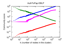
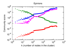
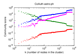
Figure 6 shows the analog of the NCP plot where now instead of conductance we use these four measures. A general observation is that modularity tends to increase roughly monotonically towards the bisection of the network. This should not be surprising since modularity measures the “volume” of communities, with (empirically, for large real-world networks) a small additive correction, and the volume clearly increases with community size. On the other hand, the modularity ratio tends to decrease towards the bisection of the network. This too should not be surprising, since it involves dividing the volume by a relatively small number. Results in Figure 6 demonstrate that, with respect to the modularity, the “best” community in any of these networks has about half of all nodes; while, with respect to the modularity ratio, the “best” community in any of these networks has two or three nodes.

Leaving aside debates about community-quality objective functions, note that, whereas the conductance and related measures are discriminative, in that they prefer different kinds of clusters, depending on the type of network being considered, modularity tends to follow the same general pattern for all of these classes of networks. That is, even aside from community-related interpretations, conductance (as well as several of the other bi-criterion objectives considered in Section 4.1) has qualitatively different types of behaviors for very different types of graphs (e.g., low-dimensional graphs, expanders, large real-world social and information networks), whereas modularity and other single-criterion objectives behave in qualitatively similar ways for all these diverse classes of graphs.

Figure 6: Four notions of community quality based on modularity. The curves do not exhibit any particularly interesting non-monotonic trends. Partitions of roughly half the network tend to have best modularity.

5 Computing lower bounds

So far we have examined various heuristics and approximation algorithms for community detection and graph partitioning. Common to these approaches is that they all only approximately find good cuts, i.e., they only approximately optimize the value of the objective function. Thus the clusters they identify provide only an upper bound on the true minimum best clusters. To get a better idea of how good those upper bounds are, we compute theoretical lower bounds. Here we discuss the spectral lower bound [6] on the conductance of cuts of arbitrary balance, and a related SDP-based lower bound [5] on the conductance of any cut that divides the graph into two pieces of equal volume.

Lower bounds are usually not computed for practical reasons, but instead are used to gain insights into partitioning algorithms and properties of graphs where algorithms perform well or poorly. Also, note that the lower bounds are “loose,” in the sense that they do not guarantee that a cluster of a particular score exists; rather they are just saying that there exists no cluster of better score.

First, we introduce the notation: $\vec{d}$ is a column vector of the graph’s node degrees; $D$ is a square matrix whose only nonzero entries are the graph’s node degrees on the diagonal; $A$ is the adjacency matrix of $G$; $L=D-A$ is then the non-normalized Laplacian matrix of $G$; 1 is vector of 1’s; and $A\bullet B=trace(A^{T}B)$ is the matrix dot-product operator. Now, consider the following optimization problem (which is well known to be equivalent to an eigenproblem):

$$\lambda_{G}={\rm min}\left\{\frac{x^{T}Lx}{x^{T}Dx}:x\perp\vec{d},x\neq 0\right\}.$$

Let $\hat{x}$ be a vector achieving the minimum value $\lambda_{G}$. Then $\frac{\lambda_{G}}{2}$ is the spectral lower bound on the conductance of any cut in the graph, regardless of balance, while $\hat{x}$ defines a spectral embedding of the graph on a line, to which rounding algorithms can be applied to obtain actual cuts that can serve as upper bounds at various sizes.

Next, we discuss an SDP-based lower bound on cuts which partition the graph into two sets of exactly equal volume. Consider:

$$\mathcal{C}_{G}={\rm min}\left\{\frac{1}{4}L\bullet Y:diag(Y)={\bf 1},Y\bullet(\vec{d}\,\vec{d}^{\,T})=0,Y\succeq 0\right\},$$

and let $\hat{Y}$ be a matrix achieving the minimum value $\mathcal{C}_{G}$. Then $\mathcal{C}_{G}$ is a lower bound on the weight of any cut with perfect volume balance, and $2\mathcal{C}_{G}/{\rm Vol}(G)$ is a lower bound on the conductance of any cut with perfect volume balance. We briefly mention that since $Y\succeq 0$, we can view $Y$ as a Gram matrix that can be factored as $RR^{T}$. Then the rows of $R$ are the coordinates of an embedding of the graph on a hypersphere. Again, rounding algorithms can be applied to the embedding to obtain actual cuts that can serve as upper bounds.

The spectral and SDP embeddings defined here were the basis for the extensive experiments with global spectral partitioning methods that were alluded to in Section 3. In this section, it is the lower bounds that concern us. Figure 7 shows the spectral and SDP lower bounds for three example graphs. The spectral lower bound, which applies to cuts of any balance, is drawn as a horizontal red line which appears near the bottom of each plot. The SDP lower bound, which only applies to cuts separating a specific volume, namely ${\rm Vol}(G)/2$, appears as an red triangle near the right side of the each plot. (Note that plotting this point required us to use volume rather than number of nodes for the x-axis of these plots.)

Clearly, for these graphs, the lower bound at ${\rm Vol}(G)/2$, is higher than the spectral lower bound which applies at smaller scales. More importantly, the lower bound at ${\rm Vol}(G)/2$, is higher than our upper bounds at many smaller scales. This demonstrates two important points: (1) It shows that best conductance clusters are orders of magnitude better than best clusters consisting of half the edges; and (2) It demonstrates that graph partitioning algorithms perform well at various size scales. For all graph partitioning algorithms, the minimum of their NCP plot is close to the spectral lower bound, and the clusters at half the volume are again close to theoretically best possible clusters. This suggests that graph partitioning algorithms we considered here do a good job both at finding best possible clusters and at bisecting the network.

Figure 7: Lower bounds on best conductance cut. In black we plot conductance curves as obtained by Local Spectral and Metis+MQI. Lower bounds on conductance of any cut (Spectral lower bound, dashed line) and the cut separating the graph in half (SDP lower bound, red triangle) show that both algorithms do a good job on finding best possible and best balanced cut of the network.

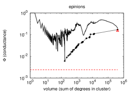
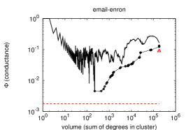
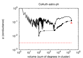
Take, for example, the first plot of Figure 7, where in black we plot the conductance curves obtained by our (Local Spectral and Metis+MQI) algorithms. With a red dashed line we plot the lower bound on the best possible cut in the network, and with red triangle we plot the lower bound for the cut that separates the graph in two equal volume parts. Thus, the true conductance curve (which is intractable to compute) lies below black but above red line and red triangle. From practical perspective this demonstrates that the graph partitioning algorithms (Local Spectral and Metis+MQI in particular) do a good job of extracting clusters at all size scales. The lower bounds tell us that the conductance curve which starts at upper left corner first has to go down and reach the minimum close to the horizontal dashed line (Spectral lower bound) and then sharply rise and ends up above the red triangle (SDP lower bound). This verifies several things: (1) graph partitioning algorithms perform well at all size scales, as the extracted clusters have scores close to the theoretical optimum; (2) the qualitative shape of the NCP is not an artifact of graph partitioning algorithms or particular objective functions, but rather it is an intrinsic property of these large networks; and (3) the lower bounds at half the size of the graph indicate that our inability to find large good-conductance communities is not a failings of our algorithms. Instead such large good-conductance “communities” simply do not exist in these networks.

Finally, in Table 1 we list for about 40 graphs the spectral and SDP lower bounds on overall conductance and on volume-bisecting conductance, and also the ratio between the two. It is interesting to see that for these graphs this ratio of lower bounds does a fairly good job of discriminating between declining-NCP-plot graphs, which have a small ratio, and V-shape-NCP-plot graphs, which have a large ratio. Small networks (like CollegeFootball, ZacharyKarate and MonksNetwork) have downward NCP plot [27, 26] and a small ratio of the SDP and Spectral lower bounds. On the other hand large networks (e.g., Epinions or Answers-3) have downward and then upward NCP plot (as in Figure 1(right)) have large ratio of the two lower bounds. This hints that in small networks “large” clusters (i.e., clusters of around half the network) tend to have best conductances. On the contrary, in large networks small clusters have good conductances, while large clusters (of the half the network size) tend to have much worse conductances, and thus high ratios of lower bounds as shown in the left table of Table 1.

	Spectral	SDP	ratio
	lowerbnd	lowerbnd	of
	on $\phi$,	on $\phi$, at	lower
Network	any size.	${\rm Vol}(G)/2$	bnds
CollegeFootball [newman_netdata]	0.068402	0.091017	1.330624
MonksNetwork [newman_netdata]	0.069660	0.117117	1.681269
ZacharyKarate [newman_netdata]	0.066136	0.127625	1.929736
PowerGrid	0.000136	0.000268	1.978484
PoliticalBooks [newman_netdata]	0.018902	0.038031	2.011991
PoliticalBlogs [newman_netdata]	0.040720	0.084052	2.064157
RB-Hierarchical [ravasz03_hierarchical]	0.011930	0.030335	2.542792
Email-InOut	0.038669	0.113367	2.931752
NetworkScience [newman_netdata]	0.001513	0.004502	2.974695
As-Oregon	0.012543	0.042976	3.426417
Blog-nat05-6m	0.031604	0.108979	3.448250
Imdb-India	0.009104	0.033318	3.659573
Cit-hep-ph	0.007858	0.029243	3.721553
Bio-Proteins	0.033714	0.126137	3.741358
As-RouteViews	0.018681	0.070462	3.771821
Gnutella-31	0.029946	0.118711	3.964127
Imdb-Japan	0.003327	0.013396	4.026721
Gnutella-30	0.030621	0.124929	4.079853
DolphinsNetwork [newman_netdata]	0.019762	0.103676	5.246171
As-Newman	0.009681	0.058952	6.089191
AtP-gr-qc	0.000846	0.006040	7.141270
Cit-hep-th	0.009193	0.068880	7.492522
AtP-cond-mat	0.001703	0.013452	7.897650

	Spectral	SDP	ratio
	lowerbnd	lowerbnd	of
	on $\phi$,	on $\phi$, at	lower
Network	any size.	${\rm Vol}(G)/2$	bnds
Gnutella-25	0.014185	0.131032	9.237332
Answers-2	0.009660	0.107422	11.120081
CA-cond-mat	0.003593	0.047064	13.098027
Answers-1	0.011896	0.159251	13.386528
Imdb-France	0.003462	0.048010	13.867591
Answers-5	0.008714	0.124703	14.311255
Imdb-Mexico	0.003893	0.070345	18.067513
CA-gr-qc	0.000934	0.017421	18.659710
AtP-hep-th	0.000514	0.009714	18.899660
AtP-hep-ph	0.000723	0.013770	19.040287
Imdb-WGermany	0.003025	0.065158	21.538867
AtP-astro-ph	0.001183	0.027256	23.036835
CA-hep-th	0.001561	0.041125	26.350412
CA-astro-ph	0.003143	0.086890	27.648094
Imdb-UK	0.001283	0.036572	28.514376
Imdb-Germany	0.000661	0.021017	31.810460
Blog-nat06all	0.002361	0.092908	39.350874
Imdb-Italy	0.000679	0.031954	47.077242
Email-Enron	0.001763	0.089876	50.965424
CA-hep-ph	0.000889	0.052249	58.755927
Epinions	0.002395	0.150242	62.739252
Answers-3	0.002636	0.185340	70.306807
Imdb-Spain	0.000562	0.046327	82.397702

Table 1: Lower bounds on the conductance for our network datasets. Spectral lower bound applies to any cut, while the SDP lower bound applies to cuts at a specified volume fraction, taken here to be half. As small networks have low ratio of lower bounds, large networks have much higher ratios which demonstrates that in large networks good clusters tend to be relatively small. Description and the statistics of the networks are available at supporting website: http://snap.stanford.edu/ncp.

6 Conclusion

In this paper we examined in a systematic way a wide range of network community detection methods originating from theoretical computer science, scientific computing, and statistical physics. Our empirical results demonstrate that determining the clustering structure of large networks is surprisingly intricate. In general, algorithms nicely optimize the community score function over a range of size scales, and the scores of obtained clusters are relatively close to theoretical lower bounds. However, there are classes of networks where certain algorithms perform sub-optimally. In addition, although many common community quality objectives tend to exhibit similar qualitative behavior, with very small clusters achieving the best scores, several community quality metrics such as the commonly-used modularity behave in qualitatively different ways.

Interestingly, intuitive notions of cluster quality tend to fail as one aggressively optimizes the community score. For instance, by aggressively optimizing conductance, one obtains disconnected or barely-connected clusters that do not correspond to intuitive communities. This suggests the rather interesting point (that we described in Section 3.1) that approximate optimization of the community score introduces a systematic bias into the extracted clusters, relative to the combinatorial optimum. Many times, as in case of Local Spectral, such bias is in fact preferred since the resulting clusters are more compact and thus correspond to more intuitive communities. This connects very nicely to regularization concepts in machine learning and data analysis, where separate penalty terms are introduced in order to trade-off the fit of the function to the data and its smoothness. In our case here, one is trading off the conductance of the bounding cut of the cluster and the internal cluster compactness. Effects of regularization by approximate computation are pronounced due to the extreme sparsity of real networks. How to formalize a notion of regularization by approximate computation more generally is an intriguing question raised by our findings.

References

- [1] Supporting website. http://snap.stanford.edu/ncp/.
- [2] R. Andersen, F. Chung, and K. Lang. Local graph partitioning using PageRank vectors. In FOCS ’06: Proceedings of the 47th Annual IEEE Symposium on Foundations of Computer Science, pages 475–486, 2006.
- [3] R. Andersen and K. Lang. Communities from seed sets. In WWW ’06: Proceedings of the 15th International Conference on World Wide Web, pages 223–232, 2006.
- [4] S. Arora, S. Rao, and U. Vazirani. Expander flows, geometric embeddings and graph partitioning. In STOC ’04: Proceedings of the 36th annual ACM Symposium on Theory of Computing, pages 222–231, 2004.
- [5] S. Burer and R. Monteiro. A nonlinear programming algorithm for solving semidefinite programs via low-rank factorization. Mathematical Programming (series B), 95(2):329–357, 2003.
- [6] F. Chung. Spectral graph theory, volume 92 of CBMS Regional Conference Series in Mathematics. American Mathematical Society, 1997.
- [7] A. Clauset. Finding local community structure in networks. Physical Review E, 72:026132, 2005.
- [8] A. Clauset, M. Newman, and C. Moore. Finding community structure in very large networks. Physical Review E, 70:066111, 2004.
- [9] I. Dhillon, Y. Guan, and B. Kulis. Weighted graph cuts without eigenvectors: A multilevel approach. IEEE Transactions on Pattern Analysis and Machine Intelligence, 29(11):1944–1957, 2007.
- [10] G. Flake, S. Lawrence, and C. Giles. Efficient identification of web communities. In KDD ’00: Proceedings of the 6th ACM SIGKDD International Conference on Knowledge Discovery and Data Mining, pages 150–160, 2000.
- [11] G. Flake, R. Tarjan, and K.Tsioutsiouliklis. Graph clustering and minimum cut trees. Internet Mathematics, 1(4):385–408, 2003.
- [12] S. Fortunato. Community detection in graphs. arXiv:0906.0612, June 2009.
- [13] S. Fortunato and M. Barthélemy. Resolution limit in community detection. Proceedings of the National Academy of Sciences of the United States of America, 104(1):36–41, 2007.
- [14] M. Gaertler. Clustering. In U. Brandes and T. Erlebach, editors, Network Analysis: Methodological Foundations, pages 178–215. Springer, 2005.
- [15] G. Gallo, M. Grigoriadis, and R. Tarjan. A fast parametric maximum flow algorithm and applications. SIAM Journal on Computing, 18(1):30–55, 1989.
- [16] M. Girvan and M. Newman. Community structure in social and biological networks. Proceedings of the National Academy of Sciences of the United States of America, 99(12):7821–7826, 2002.
- [17] R. Guimerà, M. Sales-Pardo, and L. Amaral. Modularity from fluctuations in random graphs and complex networks. Physical Review E, 70:025101, 2004.
- [18] R. Kannan, S. Vempala, and A. Vetta. On clusterings: Good, bad and spectral. Journal of the ACM, 51(3):497–515, 2004.
- [19] B. Karrer, E. Levina, and M. Newman. Robustness of community structure in networks. Physical Review E, 77:046119, 2008.
- [20] G. Karypis and V. Kumar. A fast and high quality multilevel scheme for partitioning irregular graphs. SIAM Journal on Scientific Computing, 20:359–392, 1998.
- [21] A. Lancichinetti and S. Fortunato. Community detection algorithms: a comparative analysis. arXiv:0908.1062, August 2009.
- [22] K. Lang and S. Rao. Finding near-optimal cuts: an empirical evaluation. In SODA ’93: Proceedings of the 4th annual ACM-SIAM Symposium on Discrete algorithms, pages 212–221, 1993.
- [23] K. Lang and S. Rao. A flow-based method for improving the expansion or conductance of graph cuts. In IPCO ’04: Proceedings of the 10th International IPCO Conference on Integer Programming and Combinatorial Optimization, pages 325–337, 2004.
- [24] T. Leighton and S. Rao. An approximate max-flow min-cut theorem for uniform multicommodity flow problems with applications to approximation algorithms. In FOCS ’88: Proceedings of the 28th Annual Symposium on Foundations of Computer Science, pages 422–431, 1988.
- [25] T. Leighton and S. Rao. Multicommodity max-flow min-cut theorems and their use in designing approximation algorithms. Journal of the ACM, 46(6):787–832, 1999.
- [26] J. Leskovec, K. Lang, A. Dasgupta, and M. Mahoney. Community structure in large networks: Natural cluster sizes and the absence of large well-defined clusters. arXiv:0810.1355, October 2008.
- [27] J. Leskovec, K. Lang, A. Dasgupta, and M. Mahoney. Statistical properties of community structure in large social and information networks. In WWW ’08: Proceedings of the 17th International Conference on World Wide Web, pages 695–704, 2008.
- [28] M. Newman. Modularity and community structure in networks. Proceedings of the National Academy of Sciences of the United States of America, 103(23):8577–8582, 2006.
- [29] M. Newman and M. Girvan. Finding and evaluating community structure in networks. Physical Review E, 69:026113, 2004.
- [30] F. Radicchi, C. Castellano, F. Cecconi, V. Loreto, and D. Parisi. Defining and identifying communities in networks. Proceedings of the National Academy of Sciences of the United States of America, 101(9):2658–2663, 2004.
- [31] S. Schaeffer. Graph clustering. Computer Science Review, 1(1):27–64, 2007.
- [32] J. Shi and J. Malik. Normalized cuts and image segmentation. IEEE Transcations of Pattern Analysis and Machine Intelligence, 22(8):888–905, 2000.
- [33] D. Spielman and S.-H. Teng. Spectral partitioning works: Planar graphs and finite element meshes. In FOCS ’96: Proceedings of the 37th Annual IEEE Symposium on Foundations of Computer Science, pages 96–107, 1996.
- [34] S. White and P. Smyth. A spectral clustering approach to finding communities in graphs. In SDM ’05: Proceedings of the 5th SIAM International Conference on Data Mining, pages 76–84, 2005.