An Independent Analysis of Kepler-4b through Kepler-8b$\dagger$$\dagger$affiliation: Based on archival data of the Kepler telescope.
Abstract
We present two independent, homogeneous, global analyses of the transit lightcurves, radial velocities and spectroscopy of Kepler-4b, Kepler-5b, Kepler-6b, Kepler-7b and Kepler-8b, with numerous differences over the previous methods. These include: i) improved decorrelated parameter fitting set used, ii) new limb darkening coefficients, iii) time stamps modified to BJD for consistency with RV data, iv) two different methods for compensating for the long integration time of Kepler LC data, v) best-fit secondary eclipse depths and excluded upper limits, vi) fitted mid-transit times, durations, depths and baseline fluxes for individual transits. We make several determinations not found in the discovery papers: i) We detect a secondary eclipse for Kepler-7b of depth ppm and statistical significance 3.5-. We conclude reflected light is a much more plausible origin than thermal emission and determine a geometric albedo of . ii) We find that an eccentric orbit model for the Neptune-mass planet Kepler-4b is detected at the 2- level with . If confirmed, this would place Kepler-4b in a similar category as GJ 436b and HAT-P-11b as an eccentric, Neptune-mass planet. iii) We find weak evidence for a secondary eclipse in Kepler-5b of 2- significance and depth ppm. The most plausible explanation is reflected light caused by a planet of geometric albedo . iv) A 2.6- peak in Kepler-6b TTV periodogram is detected and is not easily explained as an aliased frequency. We find that mean-motion resonant perturbers, non-resonant perturbers and a companion extrasolar moon all provide inadequate explanations for this signal and the most likely source is stellar rotation. v) We find different impact parameters relative to the discovery papers in most cases, but generally self-consistent when compared to the two methods employed here. vi) We constrain the presence of mean motion resonant planets for all five planets through an analysis of the mid-transit times. vii) We constrain the presence of extrasolar moons for all five planets. viii) We constrain the presence of Trojans for all five planets.
Subject headings:
planetary systems — stars: individual (Kepler-4, Kepler-5, Kepler-6, Kepler-7, Kepler-8) techniques: spectroscopic, photometric1. Introduction
The Kepler Mission was successfully launched on March 7th 2009 and began science operations on May 12th of the same year. Designed to detect Earth-like transits around Sun-like stars, the required photometric precision is at the level of ppm over 6.5 hours integration on 12th magnitude stars and early results indicate this impressive precision is being reached (Borucki et al., 2009). In 2010, the first five transiting exoplanets (TEPs) to be discovered by the Kepler Mission were announced by the Kepler Science Team (Borucki et al., 2010a), known as Kepler-4b, Kepler-5b, Kepler-6b, Kepler-7b and Kepler-8b (Borucki et al. (2010b); Koch et al. (2010); Dunham et al. (2010); Latham et al. (2010); Jenkins et al. (2010a)). These expanded the sample of known transiting exoplanets to about 75 at the time of announcement.
The main objective of the Kepler Mission is to discover Earth-like planets, but the instrument naturally offers a vast array of other science opportunities including detection of gas giants, searches for thermal emission (Deming et al., 2005) and/or reflection from exoplanets, detection of orbital phase curves (Knutson et al., 2007) and ellipsoidal variations (Welsh et al., 2010), asteroseismology (Christensen-Dalsgaard et al., 2010) and transit timing (Agol et al., 2005), to name a few. Confirmation and follow-up of exoplanet transits is known to be a resource intensive activity and since the detection of new planets is Kepler’s primary objective, it is logical for many of these other scientific tasks to be conducted by the astronomical community as a whole.
Independent and detailed investigations of the Kepler photometry provides an “acid-test” of the methods employed by the Kepler Science Team. Indeed, the distinct analysis of any scientific measurement has always been a fundamental corner stone of the scientific method. In this paper, we present two independent analyses of the discovery photometry for the first five Kepler planets. We aim to not only test the accuracy of the methods used in the discovery papers, but also test our own methods by performing two separate studies. Both methods will be using the same original data, as published in the discovery papers.
Some additional data-processing tasks are run through the Kepler reduced data, which we were not used in the original analyses presented in the discovery papers, and are discussed in §3. In this section, we also discuss the generation of new limb darkening coefficients and methods for compensating for the long integration time of the Kepler long-cadence photometry. We also perform individual transit fits for all available Kepler transits in order to search for transit timing variations (TTV), transit duration variations (TDV) and other possible changes. These will be used to provide a search for perturbing planets and companion exomoons.
2. Fitting Methodology
2.1. Method A
In this work, the two of us adopt different algorithms for fitting the observational data. The first code has been written by D. Kipping and is a Markov Chain Monte Carlo (MCMC) code (for a brief introduction on this method, consult appendix A of Tegmark et al. (2004)) with a Metropolis-Hastings algorithm, written in Fortran 77/90. The lightcurve model is generated using the analytic quadratic limb darkening Mandel & Agol (2002) routine, treating the specific stellar intensity with:
| (1) |
The quadratic limb darkening coefficients and are known to be highly correlated (Pál, 2008b), but a principal component analysis provides a more efficient fitting set:
| (2) | ||||
| (3) |
We also implement conditions to ensure the brightness profile is everywhere positive and monotonically decreasing from limb to center: and (Carter et al., 2008).
Quantities relating to time differences are computed by solving the bi-quartic equation for the various true anomalies of interest following the methods detailed in Kipping (2008) and Kipping (2010a). These quantities include:
-
•
The transit duration between the first and fourth contact, .
-
•
The transit duration between the second and third contact, .
-
•
The ingress and egress transit durations, and respectively.
-
•
The secondary eclipse full duration, .
-
•
The time of the predicted secondary eclipse, .
-
•
The offset time between when the radial velocity possesses maximum gradient (for the instance closest to the time of conjunction) and the primary mid-transit, .
The latter two on this list are particularly important. For example, the RV offset time provides a strong constraint on .
The principal fitting parameters for the transit model are the orbital period, , the ratio-of-radii squared, , the Kipping (2010a) transit duration equation, , the impact parameter, , the epoch of mid-transit, and the Lagrange eccentricity parameters and . is used as it describes the duration between the planet’s centre crossing the stellar limb and exiting under the same condition and this is known to be a useful decorrelated parameter for light curve fits (Carter et al., 2008). We also note that an approximate form is required as the exact expression requires solving a bi-quartic equation which is not easily invertible. In contrast, may be inverted to provide using (Kipping, 2010a):
| (4) | ||||
| (5) |
Blending is accounted for using the prescription of Kipping & Tinetti (2010) where we modify the formulas for an independent blend rather than a self-blend. The nightside pollution effect of the planet is at least an order of magnitude below the detection sensitivity of Kepler due to the visible wavelength bandpass of the instrument. Therefore, the only blending we need account for are stellar blends. In addition, the model allows for an out-of-transit flux level () to be fitted for. Unlike method B (see later), we fix to be a constant during the entire orbital phase of the planet. Secondary eclipses are produced using the Mandel & Agol (2002) code with no limb darkening and the application of a transformation onto the secondary eclipse lightcurve which effectively squashes the depth by a ratio such that the new depth is equal to (planet dayside flux to stellar flux ratio) in the selected bandpass. This technique ensures the secondary eclipse duration and shape are correctly calculated. The observed flux is therefore modeled as:
| (6) |
This model so far accounts for primary and secondary eclipses but an additional subroutine has been written to model the radial velocity variations of a single planet. Modeling the RV in conjunction with the transit data gives rise to several potential complications. Firstly, we could try fits using either an eccentric orbit or a fixed circular orbit model. An eccentric fit will always find a non-zero eccentricity due to the boundary condition that (Lucy & Sweeney, 1971). The effects of fitting versus not-fitting for eccentricity are explored in this work by presenting both fits for comparison.
A second complication is the possible presence of a linear drift in the RVs due a distant massive planet. This drifts can give rise to artificial eccentricity if not accounted for but their inclusion naturally increases the uncertainty on all parameters coming from the RV fits. Thirdly, an offset time, , between when then RV signal has maximum gradient (for the instance nearest the time of conjunction) and the mid-transit time can be included. For eccentric orbits, a non-zero offset always exists due to the orbital eccentricity. In our code this is calculated and denoted as and is calculated exactly by solving for the relevant true anomalies and computing the time interval using the duration function of Kipping (2008). However, an additional offset can also exist, , which may due to a massive body in a Trojan orbit (i.e. we have ). This offset was first predicted by Ford & Holman (2007) and the detection of a non-zero value of would indicate a Trojan. For eccentric orbits, the error in is often very large and dominates the error budget in , washing out any hints of a Trojan.
The question exists as to when one should include these two additional parameters. Their perenial inclusion would result in very large errors for poorly characterized orbits and this is clearly not desirable. We therefore choose to run a MCMC + simplex fit for all possible models and extract the lowest for the RV signal. This minimum is then used to compute the Bayesian Information Criterion, or BIC (see Schwarz (1978); Liddle (2007)). BIC compares models with differing numbers of free parameters (), heavily penalizing those with more and the preferred model is given that yielding the lowest BIC, where:
| (7) |
Where is the number of data points. In total, there exists four possible models for the circular and four possible models for the eccentric fit by switching on/off these two parameters. For both the circular and eccentric fits, we select the model giving the lowest BIC. Therefore, if for example the lowest BIC was that of a zero but non-zero , we would fix the gradient term but let the offset be freely fitted in the final results. The results of these preliminary investigations can be found in Table 14 of the Appendix.
The favored solution is generally the eccentric model over the circular model. This is because the light curve derived stellar density, which we will later use in our stellar evolution models, has a strong dependence on the eccentricity. In general, fixing leads to unrealistically small error on . However, in some cases sparse RV phase coverage can lead to artificially large values.
The code is executed as a global routine, fitting all the RV and photometry simultaneously with a total of free parameters: , , , , , , , , , , , and . The inclusion of and is reviewed on a case-by-case basis, as discussed. Additionally, the blending factor, which we denote as , is allowed to float around its best fit value in a Gaussian distribution of standard deviation equal to the uncertainty in . These values are reported in the original discovery papers.
The final fit is then executed with 125,000 trials with the first 20% of trials discarded to allow for burn-in. This leaves us with 100,000 trials to produce each a posteriori distribution, which is more than adequate. The Gelman & Rubin (1992) statistic is calculated for all fitted parameters to ensure good mixing. The final quoted values are given by the median of the resultant MCMC trials. We define the posian and negian as the maximum and minimum confidence limits of the median respectively. The negian may be found by sorting the list and extracting the entry which is 34.13% of the total list length. The posian is given by the entry which occurs at 68.27% of the total list length. These values may be then be used to determine the confidence bounds on the median.
After the global fitting is complete, we produce the distribution of the lightcurve derived stellar density and a Gaussian distribution for the SME-derived effective temperature and metallicity around the values published in the discovery papers and based on SME analysis of high resolution spectra. These distributions consist of 100,000 values and thus may be used to derive 100,000 estimates of the stellar properties through a YY-isochrone analysis (Yi et al., 2001). For errors in and , we frequently adopted double that which was quoted in the discovery papers, as experience with HAT planets has revealed that SME often underestimates these uncertainties. Finally, the planetary parameters and their uncertainties were derived by the direct combination of the a posteriori distributions of the lightcurve, RV and stellar parameters. The stellar jitter squared is found by taking the best-fit RV model residuals and calculating the variance and subtracting the sum of the measurement uncertainties squared.
2.2. Method B
The second method builds on the codes developed under the HATNet project, mostly written in C and shell scripts. These have been used for the analysis of HATNet planet discoveries, such as Pál et al. (2008a); Bakos et al. (2009); Pál (2009b), and have been heavily modified for the current case of Kepler analysis. We used a model for describing the flux of the star plus planet system through the full orbit of the planet, from primary transit to occultation of the planet. In our initial analysis we assumed a periodic model, and later we considered the case of variable parameters as a function of transit number. The flux was a combination of three terms:
| (8) | |||||
Here (the first term) is the brightness (phase-curve) of the star+planet+blend system without the effect of the transit and occultation. The drop in flux due to the transit is reflected by the second term, and the equivalent drop due to the occultation of the planet by the third term. The phase-curve is a rather simple step-function of three levels; within times the duration of the transit around the transit center, within times the duration of the occultation around the center of the occultation, and in between. For simplicity, we adopted . Because the transit and occultation centers and durations also enter the formula, depends on a number of other parameters, namely the time, mid-transit time, period, the parameter that is characteristic of the duration of the transit, planet to star radius ratio, impact parameter, and and Lagrangian orbital parameters. The location and total duration of the transit and occultation are fully determined by the above parameters. In general, the combined brightness of the star plus planet would smoothly vary from outside of the primary transit to outside of the occultation, typically as a gradual brightening as the planet shows its star-lit face towards the observer. If the night-side brightness of the planet is (Kipping & Tinetti, 2010), and the day-side brightness of the planet is , and is the flux of a blend contributing light to the system, then and (both equations normalized by ), i.e. there is a constraint between and . The reason for introducing all three of , and for characterizing the data was because the Kepler lightcurve, as provided by the archive, was “de-trended”, removing the (possible) brightening of the phase-curve due to the planet. Because of this, we found that introducing a more complex phase function was not warranted. We note that while such de-trending may be necessary to eliminate systematic effects, it also removes real physical variations of small amplitude.

The second term characterizes the dimming of the combined light of the star, blend and planet during the primary transit. The loss of stellar flux was modeled using the analytic formula based on Mandel & Agol (2002) for the eclipse of a star by a planet (Bakos et al., 2009), where the stellar flux was described by quadratic limb-darkening. The quadratic limb-darkening coefficients were derived by evaluating the stellar flux as a function of (where is the angle between the stellar surface normal vector and the line-of-sight) using the quadratic , coefficients. The formula takes into account the blending (constant flux contribution by other sources), the night-side illumination of the planet (normalized by ), and the out-of-transit flux level that was normalized by an arbitrary constant.111Had the flux been normalized by the brightness of the star, without blending and other sources, would hold.
Finally, the third term characterizes the dimming of the combined light of the star, blend and planet during the occultation of the planet. The day-side flux of the planet is gradually lost as it moves behind the star. This is modeled by a zero limb-darkening model of the secondary eclipse using the same Mandel & Agol (2002) formalism. This term also takes into account the blending, and the daytime flux of the system.
Our global modeling also included the radial velocity data. Following the formalism presented by Pál (2009), the RV curve was parametrized by an eccentric Keplerian orbit with semi-amplitude , Lagrangian orbital elements , and systemic velocity .
The Kepler photometry and radial velocity data are connected in a number of ways. For example, we assumed that there is a strict periodicity in the individual transit times222Note that we also performed a global analysis under method B by allowing the parameters of the individual transits (such as the transit centers) to vary., and the same and ephemeris of the system describes the photometric and RV variations. Another example: the Lagrangian orbital parameters and were not only determined by the RV data, but also by the phase of the occultation of the planets in the Kepler data.
Altogether, the 13 parameters describing the physical model were (the of the first transit in the Kepler data), (the same parameter for the last transit), , , , , , , , , , , and . The blending factor was kept fixed at the values published in the Kepler discovery papers (Borucki et al. (2010b); Koch et al. (2010); Dunham et al. (2010); Latham et al. (2010); Jenkins et al. (2010a)). We adopted for the night-side emission of the planet. Fitting for and would require data with exceptional quality.
The joint fit on the photometry and radial velocity data was performed as described in Bakos et al. (2009). We minimized in the parameter space by using a hybrid algorithm, combining the downhill simplex method (AMOEBA; see Press et al., 1992) with the classical linear least squares algorithm. Uncertainties for the parameters were derived using the Markov Chain Monte-Carlo method (MCMC, see Ford, 2006). The a priori distributions of the parameters for these chains were chosen from a generic Gaussian distribution, with eigenvalues and eigenvectors derived from the Fisher covariance matrix for the best-fit value. The Fisher covariance matrix is calculated analytically using the partial derivatives given by Pál (2009).
Stellar parameters were also determined in a Monte-Carlo fashion, using the tools and methodology described in e.g. Bakos et al. (2009). Basically, we used the MCMC distribution of and corresponding , a Gaussian distribution of and around the values published in the discovery papers and based on SME analysis of high resolution spectra. For errors in and we typically adopted double that of quoted in the discovery papers. Finally, the planetary parameters and their uncertainties were derived by the direct combination of the a posteriori distributions of the lightcurve, RV and stellar parameters.
Throughout this text, the final value for any given parameter is the median of the distribution derived by the Monte-Carlo Markov Chain analysis. Error is the standard deviation around the final value. Asymmetric error-bars are given if the negative and positive standard deviations differ by 30%. Parameter tables also list the RV “jitter,” which is a component of assumed astrophysical noise intrinsic to the star that we add in quadrature to the RV measurement uncertainties in order to have from the RV data for the global fit.
2.3. Parameter variation search method
2.3.1 Individual fits
In addition to global fits, we will search for variations in the lightcurve parameters for each transit. Searching for changes in the mid-transit time, commonly known as transit timing variations (TTV), can be used to search for perturbing planets (Agol et al., 2005; Holman & Murray, 2005) or companion moons (Sartoretti & Schneider, 1999; Kipping, 2009a). Similarly, transit duration variations (TDV) provide a complementary method of searching for exomoons (Kipping, 2009a, b). We also look for depth changes and baseline variations which may aid in the analysis of any putative signals.
Transit timing and duration measurements are made by splitting the time series into individual transits and fitting independently. In these individual fits, we only fit for , , , and and float all other parameters around their global best-fit determined value with their a posteriori distribution. The limb darkening coefficients are fixed to the theoretical values for these fits, since epoch to epoch variation in the LD coefficients is not expected. We choose to use method A for the individual fits as the parameter is more likely to have a uniform prior than (as used in method B), from geometric considerations. As for the global fits, we perform 125,000 trials for each fit with the first 25,000 (20%) trials being used as a burn-in.
For the TDV, we define our transit duration as the time for the sky-projection of the planet’s center to move between overlapping the stellar disc and exiting under the same condition, . This value was first proposed by Carter et al. (2008) due to its inherently low correlations with other parameters. As a result, this definition of the duration may be determined to a higher precision than the other durations. has the property that its uncertainty is exactly twice that of the mid-transit time for a trapezoid approximated lightcurve. In reality, limb darkening will cause this error to be slightly larger. Nevertheless, this property means that a useful definition of TDV is to halve the actual variations to give TDV = where is the globally-fitted value of . The factor of 0.5 means that we expect the r.m.s. scatter of the TDV to be equal to, or slightly larger than, the TTV scatter. It is also worth noting that in reality we could use any factor we choose rather than 0.5, because TDV is really a measurement of the fractional variation in duration and is not absolute in the sense that TTV is.
2.3.2 Periodograms
When analyzing the TTV and TDV signals, we first compute the of a model defined by a static system, i.e. constant duration and linear ephemeris. This value is naturally computed from the MCMC uncertainties for each transit. In practice, these errors tend to be overestimates. This is because the MCMC only produces accurate errors if it is moving around the true global minimum. In reality, slight errors in the limb darkening laws, the finite resolution of our integration-time compensation techniques and the error in the assumed photometric weights themselves mean that our favorite solution is actually slightly offset from the true solution. Consequently, the MCMC jumps sample a larger volume of parameter space than if they were circling the true solution.
Despite the wide-spread use and therefore advocation of the MCMC method for transit analysis, it is also unclear whether the MCMC method does produce completely robust errors, particularly in light of the inevitable hidden systemic effects. Therefore searching for excess variance in the values may not be a completely reliable method of searching for signals, echoed recently by Gibson et al. (2009). Concordantly, in all of our analyses, we compare the of a static model versus that of a signal and compute the F-test. The F-test has the advantage that it does care not about the absolute values, only the relative changes. Furthermore, it penalizes models which are overly complex (Occam’s razor).
We therefore compute periodograms by moving through a range of periods in small steps of 1/1000 of the transit period and then fitting for a sinusoidal signal’s amplitude and phase in each case. We compute the of the new fit and then use an F-test to compute the false alarm probability (FAP) to give the F-test periodogram. Any peaks below 5% FAP are investigated further and we define a formal detection limit of 3- confidence. Compared to the generalized Lomb-Scargle periodogram, the F-test is more conservative as it penalizes models for being overly-complex and therefore offers a more prudent evaluation of the significance of any signal. Conceptually, we can see that the difference is that a Lomb-Scargle periodogram computes the probability of obtaining a periodic signal by chance whereas the F-test periodogram computes the statistical significance of preferring the hypothesis of a periodic signal over a null hypothesis.
2.3.3 Analysis of variance
In general, there are two types of periodic signals we are interested in searching for; those of period greater than the sampling rate (long-period signals) and those of periods shorter than the sampling rate (short-period signals). An example of a long-period signal would be an exterior perturbing planet and a short-period signal example would be a companion exomoon. Periodograms are well suited for detecting long period signals above the Nyquist frequency, which is equal to twice the sampling period. Short-period signals cannot be reliably seeked below the Nyquist frequency. First of all, a period equal to the sampling rate will always provide a strong peak. Periods of an integer fraction of this frequency will also present strong significances (e.g. 1/2, 1/3, 1/4, etc). As the interval between these aliases becomes smaller, very short-period signals become entwined. If a genuine short-period signal was present, it would exhibit at least partial frequency mixing with one of these peaks to create a plethora of short-period peaks. As a result, peaks in the periodogram below cannot be considered as evidence for authentic signals. Therefore, we only plot our periodograms in the range of to twice the total temporal coverage.
To resolve this issue, it is possible to derive an exomoon’s period by taking the ratio of the TTV to TDV r.m.s. amplitudes (Kipping, 2009a, b). Since both of these signals are very short period, the data would ostensibly be seen as excess scatter. These excess scatters can be used to infer the r.m.s. amplitude of each signal and then derive the exomoon’s period from the ratio. Excess scatter, or variance, may be searched for by applying a simple test of the data, assuming a null-hypothesis of no signal being present. If a signal is found, or we wish to place constraints on the presence of putative signal amplitudes, we use the -distribution due to both Gaussian noise plus an embedded high frequency sinusoidal signal to model the variation.
2.3.4 Phasing
An unusual aspect of the individual data sets is that consecutive data points are 30 minutes apart. Despite accounting for the long integration times in our modeling (see later in §3.5), we consider the possibility that the long cadence data could produce artificial signals in the parameter variation search. We propose that one method of monitoring the effects of the long integration time is what we denote as phasing.
Using the globally fitted ephemeris, we know the mid-transit time for all transits (assuming a non-variable system). We may compare the difference between this mid-transit time and the closest data point in a temporal sense. This time difference can take a maximum value of minutes (assuming no data gaps) and will vary from transit to transit. We label this time difference as the phasing. In all searches for parameter variations, a figure showing the phasing will also be presented. This allows us to check whether any putative signals are correlated to the phasing, which would indicate a strong probability the signal is spurious.
3. Data processing
3.1. Barycentric Julian Dates
The radial velocity data from Kepler is provided in barycentric Julian date (BJDUTC) but the photometry is given in heliocentric Julian data (HJDUTC). For consistency, we calculate the difference between HJD and BJD for every time stamp and apply the appropriate correction. We use the JPL Horizons ephemeris to perform this correction, which is important given that the difference between HJD and BJD can be a few seconds. We do not correct times from the UTC system to TDB/TT (Eastman et al., 2010) as the difference is effectively a constant systematic due to leap seconds which accumulate over decades timescale. Further, recent Kepler data products (e.g. Kepler Data Release 5) use the BJDUTC system and thus there is a preference to remain consistent with the probable future data format.
3.2. Measurement uncertainties
Unfortunately, the Kepler pipeline output did not include photometric uncertainties which forces us to evaluate the measurement errors ourselves. For Kepler-4b, Kepler-5b, Kepler-6b and Kepler-7b, we found that the r.m.s. scatter was constant over the observational period. In order to estimate the standard deviation, we use the median absolute deviation (MAD) from Gauss (1816) due to its robustness against outliers. Assuming Gaussian errors, the standard deviation is given by 1.4286 multiplied by the MAD value. This value for the standard deviation is then assigned to all data points as their measurement uncertainty.
For Kepler-8b, this approach was no possible since the r.m.s. scatter varies with time. To estimate the errors, we calculate the standard deviation using MAD in 50 point bins, excluding the transits and secondary eclipses. This binning window is shifted along by one data point and then repeated until we reach the end of the time series. The MAD-derived standard deviations are then plotted as a function of median time stamp from the binning window. Finally, we find that a quadratic fit through the data provides an excellent estimation of the trend. This formula is then used to generate all measurement uncertainties.
3.3. Outliers
Although the data has been ‘cleaned’ by the Kepler pipeline (Jenkins et al., 2010b), we run the data through a highly robust outlier detection algorithm developed by Beaulieu et al. (2010) using the MAD method. Essentially, we use MAD to estimate the standard deviation and then estimate a sigma clipping level. This is found by setting the sigma clipping level to a value such that if all the errors were Gaussian, we would only expect to reject one valid data point by accident, which is a function of the array length.
For each system we use MAD to estimate the outlier-robust standard deviation to be ppm, ppm, ppm and ppm for Kepler-4b through 7b respectively. For Kepler-8b we find that the standard deviation of the photometry is variable as described in the previous subsection. We present the list of rejected outlier points in Table 2 of the appendix.
3.4. Limb Darkening
Accurate limb darkening coefficients were calculated for the Kepler bandpass for each planet. For the Kepler-bandpass, we used the high resolution Kepler transmission function found at http://keplergo.arc.nasa.gov/CalibrationResponse.shtml. We adopted the SME-derived stellar properties reported in the original discovery papers. We employed the Kurucz (2006) atmosphere model database providing intensities at 17 emergent angles, which we interpolated linearly at the adopted and values. The passband-convolved intensities at each of the emergent angles were calculated following the procedure in Claret (2000). To compute the coefficients we considered the following expression:
| (9) |
where is the intensity, is the cosine of the emergent angle, and are the coefficients. The final coefficients resulted from a least squares singular value decomposition fit to 11 of the 17 available emergent angles. The reason to eliminate 6 of the angles is avoiding excessive weight on the stellar limb by using a uniform sampling (10 values from 0.1 to 1, plus ), as suggested by Díaz-Cordovés et al. (1995). This whole process is performed by a Fortran code written by I. Ribas (Beaulieu et al., 2010). The coefficients are given in the final parameter tables for each planet.
3.5. Integration Time
The Kepler long-cadence (LC) photometry is produced by the onboard stacking of 270 images of 6.02 seconds exposure. There is a 0.52 second read-time on-top of the exposure time which leads to a net duty-cycle of 91.4%. The duty cycle is sufficiently high that we can consider the LC photometry to be equivalent to one long exposure of 29.4244 minutes. As a result of such a long integration, sharp changes in the photometry, due to say a transit ingress, are smeared out into broader morphologies. In itself, this does not pose a problem since the nature of this smearing is well understood and easily predicted.
Kipping (2010b) discusses in detail the consequences of finite integration times, with particular focus on Kepler’s LC photometry. The effects of the smearing may be accounted for by using a time-integrated flux model for the lightcurve, as opposed to an instantaneous flux model. If we denote the flux predicted at any instant by , the time-integrated flux by and the integration time by , the observed flux will be given by:
| (10) |
Kipping (2010b) proposes two methods of numerically integrating this expression; Simpson’s composite rule and re-sampling. In this work, both of us compensate for the effect in different ways. Method A employs Simpson’s composite rule and method B employs re-sampling. In both cases, we use the expressions of Kipping (2010b), given below in equations (5) and (6) to choose our numerical resolution such that the maximum photometric error induced by the finite numerical resolution is less than the observed photometric uncertainties, as seen in Table 1.
| (11) | |||||
| (12) |
, where is the transit depth, is ingress duration, and is the integration time.
| Planet | Required for | used for | Required | used |
|---|---|---|---|---|
| Comp. Simp. Rule | Comp. Simp. Rule | for Resampling | for Resampling | |
| Kepler-4b | 0.9434 | 2 | 1.6339 | 4 |
| Kepler-5b | 1.7108 | 2 | 2.9632 | 4 |
| Kepler-6b | 2.1848 | 2 | 3.7839 | 4 |
| Kepler-7b | 1.7199 | 2 | 2.9790 | 4 |
| Kepler-8b | 1.0810 | 2 | 1.8723 | 4 |
4. Kepler-4b
4.1. Global Fits
The discovery of Kepler-4b was made by Borucki et al. (2010b). The planet is particularly interesting for joining the club of HAT-P-11b and GJ 436b as a Neptune-mass transiting exoplanet. Kepler-4b exhibits a sub-mmag transit around a magnitude star, which leads to relatively large uncertainties on the system parameters but demonstrates the impressive performance of the Kepler photometry.
However, the combination of the course sampling (e.g. the ingress/egress duration is 3-4 times shorter than the cadence of the observations), the very low RV amplitude and a sub-mmag transit make Kepler-4b the most challenging object to determine reliable system parameters for in this paper. The BIC test for the approriate RV model prefers the simplest description possible, reflecting the low signal-to-noise levels encountered for the radial velocities.
The largest difference between our own fits and that of Borucki et al. (2010b) is the retrieved and impact parameter, . Borucki et al. (2010b) find an equatorial transit solution whereas our method A circular fit, and both modes of method B, place Kepler-4b at an impact parameter of 0.5-0.6. Curiously, the eccentric fit of method A prefers an even larger impact parameter than this, as a result of letting the limb darkening be fitted.
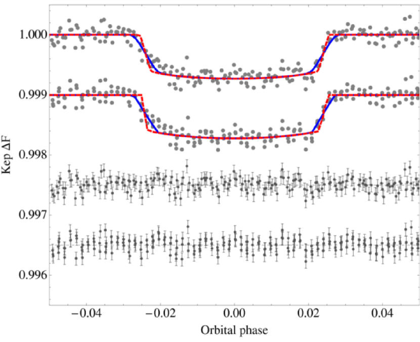
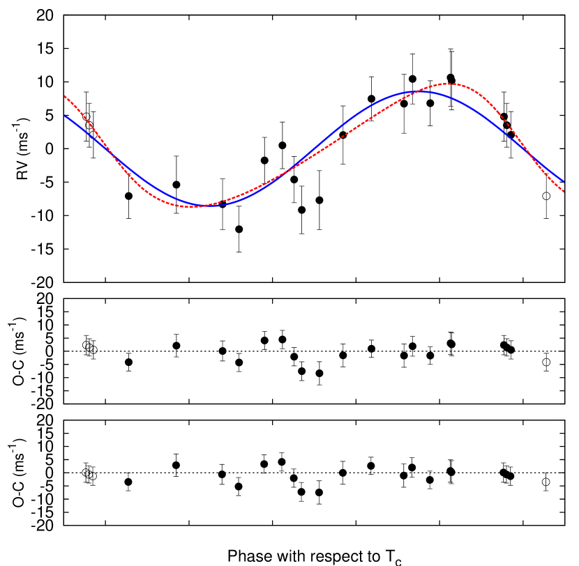
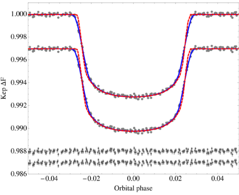
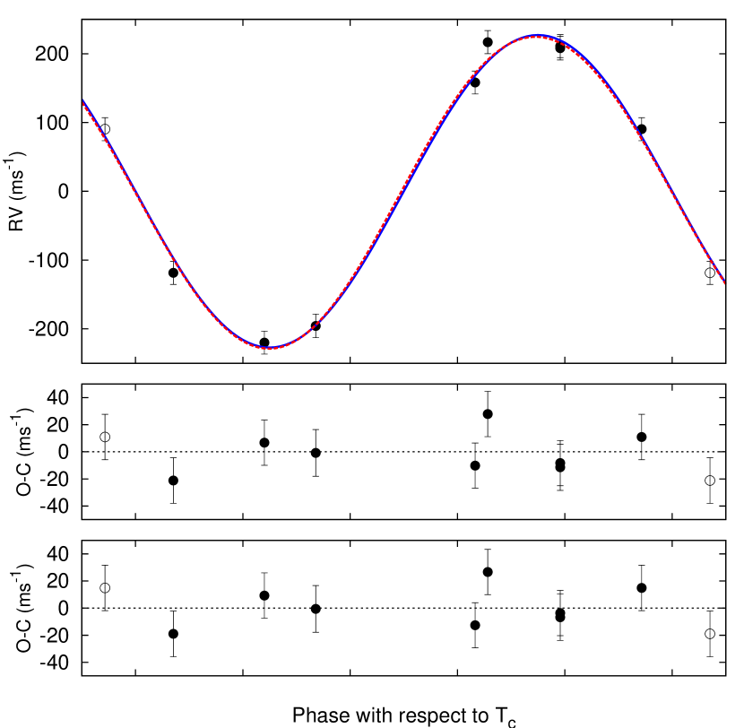
Due to the well-known negative correlation between and (Carter et al., 2008), these larger values lead to lower values and consequently a significantly lower lightcurve derived stellar density, . Indeed, the lower stellar density results in one of the largest stellar radii out of all the known transiting systems. The fitted models on the phase-folded lightcurves are shown on Figure 2 using method B. Correlated noise was checked for in the residuals using the Durbin-Watson statistic, which finds , well inside the 1% critical boundary of . The orbital fits to the RV points are shown in Fig. 3 (method B), depicting both the circular and eccentric fits. The final table of all results are shown in Table 2.
4.1.1 Eccentricity
From Table 14 of the Appendix, the circular fit with no other free parameters is the preferred model to describe the radial velocities of Kepler-4b. We may perform other tests aside from the BIC model selection though. The global circular fit, using method A, yields a and the eccentric fit obtains . These values correspond to the lowest solution of the simplex global fit, but for the RV points only, which dominate the eccentricity determination. Assuming the period and epoch are essentially completely driven by the photometry, the number of free parameters are 2 and 4 for the circular and eccentric fits respectively. Therefore, based upon an F-test, the inclusion of two new degrees of freedom to describe the eccentricity is justified at the 1.7- level (91.5% confidence). Another test we can implement is the Lucy & Sweeney (1971) test, where the significance of the eccentric fit is given by:
| (13) |
Where is the modal value of and is the error (in the negative direction). We find that this gives a significance of 88.2% or 1.6-, in close agreement with the F-test result. We also computed the posterior distribution of the distance of the pericentre passage, in units of the stellar radius, and found for method A. Therefore, if the eccentric fit is the true solution, Kepler-4b would make an extremely close pericentre passage.
We note that Borucki et al. (2010b) found a best-fit eccentricity of (no quoted uncertainty) but the authors concluded the eccentric fit was not statistically significant, but provided no quantification. Based upon the current observations, it is not possible to make a reliable conclusion as to whether Kepler-4b is genuinely eccentric or not. At best, it can be considered a - marginal detection of eccentricity. The only assured thing we can say is that to 95% confidence. Despite the ambiguity of the eccentricity, it is interesting to consider the consequences of this object possessing .
For the eccentric fit, the extreme proximity of this planet to the star raises the issue of tidal circularization. Let us continue under the assumption that no third body is responsible for pumping the eccentricity of Kepler-4b. For a planet initially with , the eccentricity decreases to after circularization timescales. This means the maximum number of circularization timescales which have transpired is given by . Since (age of the system divided by circularization timescale) then we may write . Using the method of Adams & Laughlin (2006), the tidal circularization time may be written as:
| (14) |
Given that , we may compute the minimum possible value of through re-arrangement:
| (15) |
The final term, may be neglected since we are interested in the minimum limit of and this term only acts to further increase the for non-zero . The advantage of doing this is that is a function of time and thus we can eliminate a term which would otherwise have to be integrated over time. Taking the posterior distribution of the equation for method A yields . We find that 99.9% of the MCMC trials correspond to for the eccentric fit. Thus, if the eccentric fit was genuine, Kepler-4b would exhibit very poor tidal dissipation. This is somewhat reminiscent of GJ 436b (Deming et al., 2007) and HAT-P-11b (Bakos et al., 2009) for which a large value is also predicted and raises the interesting question as to whether hot-Neptune generally possess larger values than their Jovian counterparts. We also note that WASP-18b has also been proposed to possess a greater-than-Jovian- (Hellier et al., 2009).
This discussion highlights the importance of obtaining more statistics regarding the eccentricity of transiting hot-Neptunes, which may reveal some fundamental insights into the origin of these objects.
4.1.2 Secondary eclipse
We here consider the circular model only since the eccentric fit is not unambiguously accepted. Global fits do not find any significant detection of the secondary eclipse. Secondary depths ppm are excluded to 3- confidence, which corresponds to geometric albedos greater than unity and thus this places no constraints on the detectability of reflected light from the planet. The thermal emission is limited by this constraint such that K, which places no constraints on redistribution.
4.1.3 Properties of the parent star Kepler-4
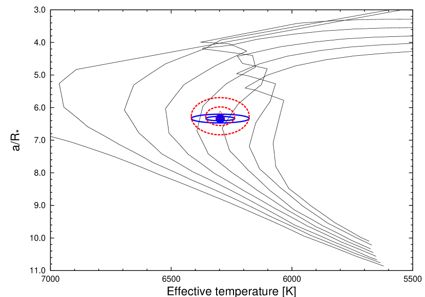
The Yonsei-Yale model isochrones from Yi et al. (2001) for metallicity = are plotted in Figure 4, with the final choice of effective temperature and marked, and encircled by the 1 and 2 confidence ellipsoids, both for the circular and the eccentric orbital solution from method B. Here the MCMC distribution of comes from the global modeling of the data. Naturally, errors of the stellar parameters for the eccentric solution are larger, due to the larger error in , which, in turn, is due to the uncertainty in the Lagrangian orbital parameters and (as opposed to fixing these to zero in the circular solution).
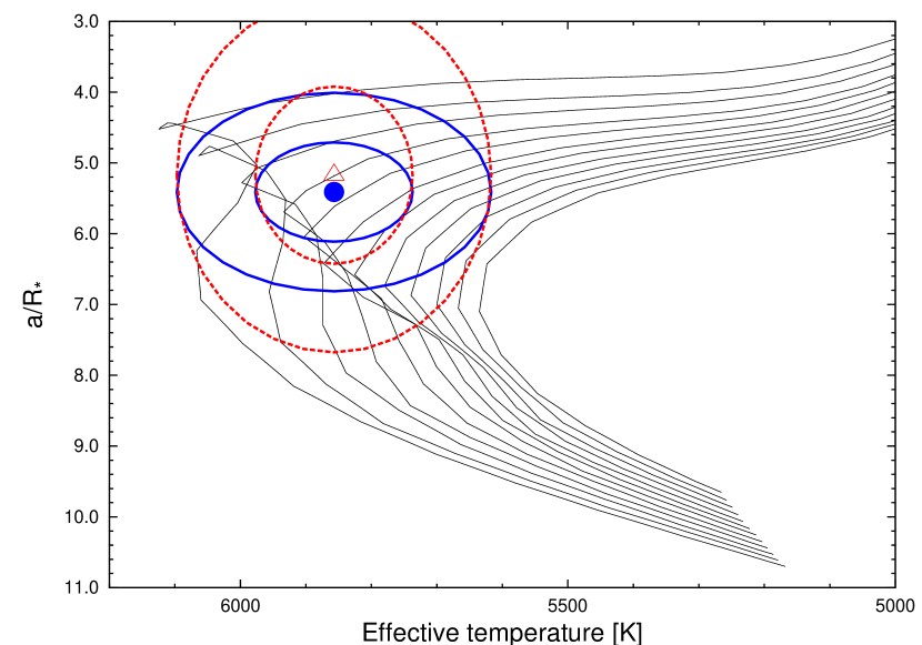
The stellar evolution modeling provides color indices that may be compared against the measured values as a sanity check. The best available measurements are the near-infrared magnitudes from the 2MASS Catalogue (Skrutskie et al., 2006). For Kepler-4, these are: , and ; which we have converted to the photometric system of the models (ESO system) using the transformations by Carpenter (2001). The resulting measured color index is . This is within 2- of the predicted value from the isochrones of (see 2). The distance to the object may be computed from the absolute magnitude from the models () and the 2MASS magnitude, which has the advantage of being less affected by extinction than optical magnitudes. The result is pc, where the uncertainty excludes possible systematics in the model isochrones that are difficult to quantify.
| Parameter | Discovery | Method A.c | Method A.e | Model B.c | Model B.e |
|---|---|---|---|---|---|
| Fitted params. | |||||
| days | |||||
| (BJD-2,454,000) | |||||
| /s | - | ||||
| /s | - | ||||
| /s | - | ||||
| /% | - | ||||
| - | |||||
| /days-1 | - | ||||
| /ppm | - | ||||
| 0∗ | 0∗ | 0∗ | |||
| 0∗ | 0∗ | 0∗ | |||
| /ms-1 | - | ||||
| /ms-1 | |||||
| /ms-1day-1 | 0∗ | 0∗ | 0∗ | 0∗ | 0∗ |
| /days | 0∗ | 0∗ | 0∗ | 0∗ | 0∗ |
| SME derived params. | |||||
| /K | |||||
| log | |||||
| (dex) | |||||
| () | |||||
| - | ∗ | ∗ | |||
| - | ∗ | ∗ | |||
| Model indep. params. | |||||
| /∘ | |||||
| 0∗ | 0∗ | 0∗ | |||
| /∘ | - | - | - | ||
| RV jitter () | - | 1.7 | 1.0 | ||
| /gcm-3 | |||||
| log | |||||
| /s | - | ||||
| /(BJD-2,454,000) | - | ||||
| Derived stellar params. | |||||
| log | |||||
| /mag | |||||
| Age/Gyr | |||||
| Distance/pc | |||||
| Derived planetary params. | |||||
| /gcm-3 | |||||
| /AU | |||||
4.2. Transit timing analysis
4.2.1 Analysis of variance
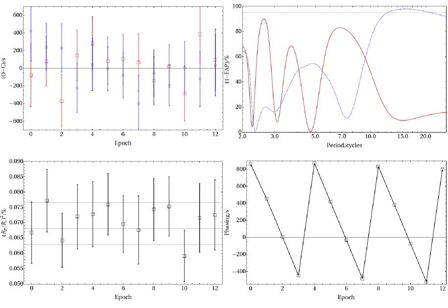
We find TTV residuals of 207.8 seconds and TDV residuals of 217.0 seconds using method A. Repeating the TTV analysis for method B finds best-fit times of consistently less than 0.25- deviance (we note that similar results were found for all planets). The TTV indicates timings consistent with a linear ephemeris, producing a of 5.7 for 11 degrees of freedom. This is somewhat low with a probability of 10.9% of occurring by coincidence. This may be an indication that the MCMC methods adopted here yield artificially large error bars, perhaps due to our choice of free-fitting every lightcurve rather than fixing certain parameters. However, we prefer to remain on the side prudence by overestimating such errors rather than underestimating them. The TDV too is consistent with a non-variable system exhibiting a of 6.4 for 12 degrees of freedom (10.6% probability of random occurrence).
Under the assumption that the timing uncertainties are accurate or overestimated, it is possible for us to determine what signal amplitudes are excluded for waveforms of a period less than the temporal baseline. For the TTV, we note that for 11 degrees of freedom, excess scatter producing a of 28.5 would be detected to 3- confidence. This therefore excludes a short-period signal of r.m.s. amplitude seconds. Similarly, for the TDV, we exclude scatter producing a of 30.1, or a short-period r.m.s. amplitude of seconds, to 3- confidence. This constitutes a 4.9% variation in the transit duration.
These limits place constraints on the presence of perturbing planets, moons and Trojans. For the case a 2:1 mean-motion resonance perturbing planet, the libration period would be cycles (2.9 years) and thus we do not possess sufficient baseline to look for such perturbers yet. However, this libration period is less than the mission lifetime of Kepler (3.5 years) and so assuming the same timing precision for all measurements, the TTV will be sensitive to a 0.14 perturber.
The current TTV data rules out an exomoon at the maximum orbital radius (for retrograde revolution) of mass . The TDV data rules an exomoon of at a minimum orbital distance.
Using the expressions of Ford & Holman (2007) and assuming , the expected libration period of Kepler-4b induced by Trojans at L4/L5 is 50.5 cycles and therefore we do not yet possess sufficient temporal baseline to look for the TTVs. However, inspection of the folded photometry at from the transit centre excludes Trojans of effective radius to 3- confidence.
4.2.2 Periodograms
As discussed in section §2.3.2, we may use an F-test periodogram to search for periodic signals, as this negates any problems introduced by underestimating or overestimating timing uncertainties. Whilst a search for excess variance is sensitive to any period below the temporal baseline, periodograms are limited to a range of .
There are no peaks in the TTV periodogram below 5% FAP. The TDV does seem to exhibit a significant peak, which can also be seen by eye in the TDV plot itself, at a period of cycles, amplitude seconds and FAP 2.1% (2.3-). A linear trend in the durations could be confused with a long period signal. Fitting a simple model yields seconds and seconds/cycle with FAP 2.6% (2.2-). Therefore, the two models yield very similar significances and it is difficult to distinguish between these two scenarios. The linear drift model seems improbable due to the very rapid change in duration the trend implies. The gradient equates to a change of around one hour per year in the half-duration, i.e. two hours per year in . The period of the signal is too large to be caused by an exomoon and TDV is generally insensitive to perturbing planets, meaning that any planet which could produce such a large effect would dominate the radial velocity. Other TDV effects, for example apsidal precession, are not expected to occur on timescales of 10-20 days which puts the reality of the signal in question.
The phasing of the measurements, as defined in §2.3.4, yields a clear periodic waveform of period 4 cycles. Therefore one possible explanation for the TDV signal is a mixing of this phasing frequency with the Nyquist frequency to produce a signal of period 16 cycles, which is consistent with the value determined earlier. The analysis of further measurements is evidently required to assess the reality of the putative signal.
4.3. Depth and OOT Variations
The transit depth is consistent with the globally fitted value yielding a of 4.3 for 12 degrees of freedom. Similarly, the OOT levels are flat yielding a of 6.1 for 12 degrees of freedom.
| Epoch | /(BJD-2,454,000) | /s | ||
|---|---|---|---|---|
| 0 | ||||
| 1 | ||||
| 2 | ||||
| 3 | ||||
| 4 | ||||
| 5 | ||||
| 6 | ||||
| 7 | ||||
| 8 | ||||
| 9 | ||||
| 10 | ||||
| 11 | ||||
| 12 |
5. Kepler-5b
5.1. Global fits
5.1.1 Comparison to discovery paper
Kepler-5b was discovered by Koch et al. (2010). Our global fits reveal Kepler-5b to be a planet on an orbit consistent with that of a circular orbit, transiting the host star at a near-equatorial impact parameter. The fitted models for method B of the phase-folded lightcurves are shown on Figure 6. Correlated noise was checked for in the residuals using the Durbin-Watson statistic, which finds , which is well within the 1% critical level of . The orbital fits to the RV points are shown in Fig. 9 for method B, depicting both the circular and eccentric solutions. We obtain transit parameters broadly consistent with that of the discovery paper, except for where method A favors an equatorial transit and method B favors a near-equatorial transit, whereas Koch et al. (2010) found . The final parameters are summarized in Table 4. Lightcurve fits reveal that the theoretical limb darkening values differ from the fitted values by a noticeable amount and the residuals of method B do reveal some structure as a consequence. Future SC mode observations will pin down the limb darkening to a much higher precision.
5.1.2 Eccentricity
The global circular fit of method A yields a for the RVs and the eccentric fit obtains . Based on an F-test, the inclusion of two new degrees of freedom to describe the eccentricity is justified below the 1- level and is therefore not significant. We therefore conclude that the system is consistent with a circular orbit and constrain to 95% confidence.
5.1.3 Secondary eclipse
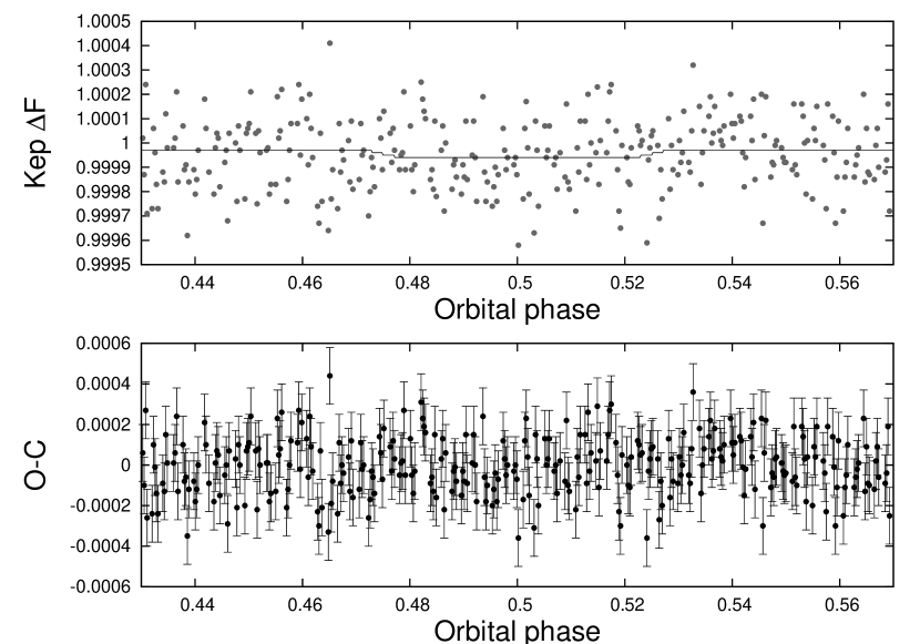
We here only consider the circular fits since the eccentric solution is not statistically significant. Method B provides the more accurate constraints due the use of multiple baseline scalings. Proceeding with method B, the secondary eclipse is weakly detected in our analysis to 93.4% confidence, or 1.8-, with a depth of ppm.
The MCMC distribution of the values is shown in Figure 8. The discovery paper reported a weak 2.0- detection of the eclipse but did not provide an amplitude for the signal. An eclipse of depth ppm is excluded at the 3- level, which excludes a geometric albedo to the same level.
If due to thermal emission, we find that by integrating a Planck function with the Kepler response function, the planetary brightness temperature would have to be K, which is inconsistent with that expected for the equilibrium temperature of K. Assuming negligible albedo and solving for the redistribution factor implies a factor of 3.7, which surpasses the maximal physically permitted value of 8/3 (corresponding to 2300K). Internal heating also seems to be unlikely as the heat source would have to be able to generate a surface temperature of 2300 K alone, or have an intrinsic luminosity of which is approximately that of a M7V star. Tidal heating from eccentricity seems improbable given that the orbit is consistent with a circular orbit. However, using our best-fit eccentricity and the equations of Peale & Cassen (1978), we estimate that tidal heating could induce for and . In order to get enough tidal heating, we require , which is much less than the typical values expected. Furthermore, such a low leads to very rapid circularization which somewhat nullifies the argument.
If the eclipse was due to reflection, we estimate a required geometric albedo of . This latter option does offer a plausible physical origin for the secondary eclipse and therefore should be considered as a possible explanation for the observation. Although there has been a general impression that hot-Jupiters must have low albedos after the remarkable MOST constraints of for HD 209458b by Rowe et al. (2008), a recent study by Cowan & Agol (2010) finds evidence for hot-Jupiters having much higher albedos () in a statistical sample of 20 exoplanets. Therefore, a geometric albedo of 0.15 is not exceptional in such a sample and offers much more reasonable explanation that thermal emission. However, at this stage, the 2- significance is too low to meet the requirements for formal detection.

5.1.4 Properties of the parent star Kepler-5
The Yonsei-Yale model isochrones from Yi et al. (2001) for metallicity = are plotted in Figure 10, with the final choice of effective temperature and marked, and encircled by the 1 and 2 confidence ellipsoids, both for the circular and the eccentric orbital solution. Here the MCMC distribution of comes from the global modeling of the data.
| Parameter | Discovery | Method A.c | Method A.e | Model B.c | Model B.e |
|---|---|---|---|---|---|
| Fitted params. | |||||
| days | |||||
| (BJD-2,454,000) | |||||
| /s | - | ||||
| /s | - | ||||
| /s | - | ||||
| /% | - | ||||
| - | |||||
| /days-1 | - | ||||
| /ppm | - | ||||
| 0∗ | 0∗ | 0∗ | |||
| 0∗ | 0∗ | 0∗ | |||
| /ms-1 | |||||
| /ms-1 | |||||
| /ms-1day-1 | 0∗ | 0∗ | 0∗ | ||
| /days | 0∗ | 0∗ | 0∗ | 0∗ | 0∗ |
| SME derived params. | |||||
| /K | |||||
| log | |||||
| (dex) | |||||
| () | |||||
| - | ∗ | ∗ | |||
| - | ∗ | ∗ | |||
| Model indep. params. | |||||
| /∘ | |||||
| 0∗ | 0∗ | 0∗ | |||
| /∘ | - | - | - | ||
| RV jitter () | - | 8.2 | 7.7 | ||
| /gcm-3 | |||||
| log | |||||
| /s | - | ||||
| /(BJD-2,454,000) | - | ||||
| Derived stellar params. | |||||
| log | |||||
| /mag | - | ||||
| Age/Gyr | |||||
| Distance/pc | - | ||||
| Derived planetary params. | |||||
| /gcm-3 | |||||
| /AU | |||||
5.2. Transit timing analysis
5.2.1 Analysis of variance
We find TTV residuals of 30.1 seconds and TDV residuals of 35.6 seconds. The TTV indicates timings consistent with a linear ephemeris, producing a of 8.7 for 10 degrees of freedom. The TDV is also consistent with a non-variable system exhibiting a of 10.5 for 11 degrees of freedom.
For the TTV, we note that for 10 degrees of freedom, excess scatter producing a of 26.9 would be detected to 3- confidence. This therefore excludes a short-period signal of r.m.s. amplitude seconds. Similarly, for the TDV, we exclude scatter producing a of 28.5, or a short-period r.m.s. amplitude of seconds, to 3- confidence. This constitutes a 0.60% variation in the transit duration.
These limits place constraints on the presence of perturbing planets, moons and Trojans. For the case a 2:1 mean-motion resonance perturbing planet, the libration period would be cycles and thus we do not possess sufficient temporal baseline to look for such perturbers yet. However, a 3:2 resonance would produce a libration period of 15.4 cycles and thus we would expect the effects to be visible over the 12 observed cycles so far. This therefore excludes a 3:2 resonant perturber of mass to 3- confidence.
The current TTV data rules out an exomoon at the maximum orbital radius (for retrograde revolution) of . The current TDV data rules an exomoon of at a minimum orbital distance.
Using the expressions of Ford & Holman (2007) and assuming , the expected libration period of Kepler-5b induced by Trojans at L4/L5 is 10.0 cycles and therefore we can search for such TTVs. We find such Trojans of cumulative mass at angular displacement are excluded by our timings. Inspection of the folded photometry at from the transit centre excludes Trojans of effective radius to 3- confidence.
5.2.2 Periodograms
An F-test periodogram of the TTV reveals only one significant peaks which is very close to Nyquist frequency. We therefore disregard this frequency as being significant.
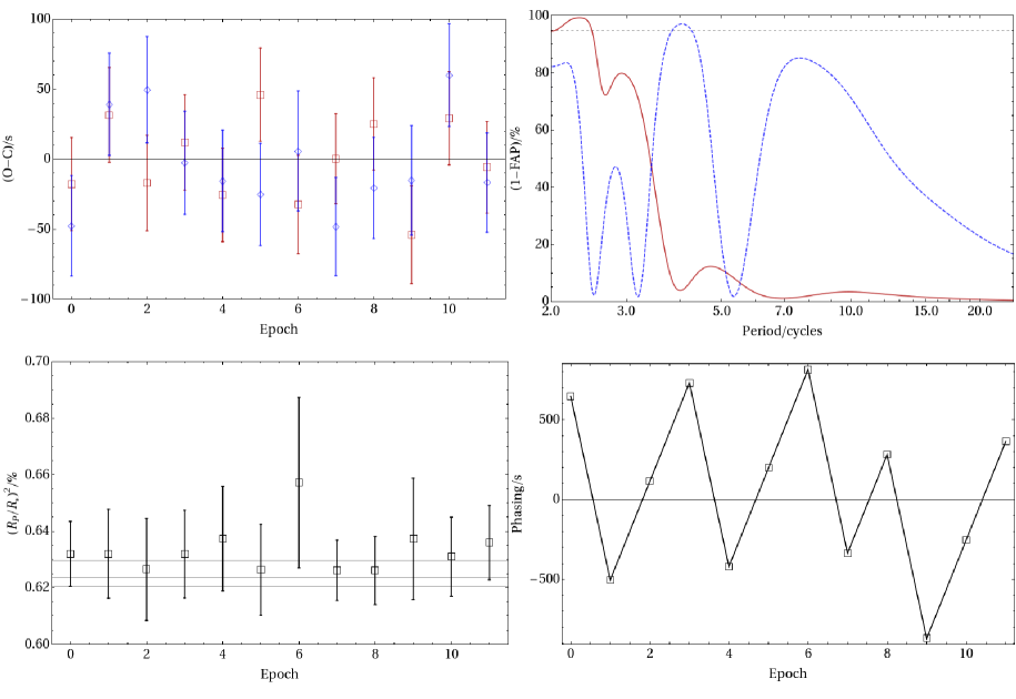
The TDV F-test periodogram reveals a significant peak at cycles with amplitude seconds with significance 2.2-. We again note that the period is not in the range which would be expected due to the known physical sources. The phasing effect has a period of 3 cycles and thus a mixing between the phasing and Nyquist frequency again offers a reasonable explanation for this signal, especially since peaks occur at 2 and 3 cycles in the TDV periodogram as well.
5.3. Depth and OOT Variations
The transit depth is consistent with the globally fitted value yielding a of 7.9 for 11 degrees of freedom. Similarly, the OOT levels are flat yielding a of 4.0 for 11 degrees of freedom.
| Epoch | /(BJD-2,454,000) | /s | ||
|---|---|---|---|---|
| 0 | ||||
| 1 | ||||
| 2 | ||||
| 3 | ||||
| 4 | ||||
| 5 | ||||
| 6 | ||||
| 7 | ||||
| 8 | ||||
| 9 | ||||
| 10 | ||||
| 11 |
6. Kepler-6b
6.1. Global Fits
6.1.1 Comparison to the discovery paper
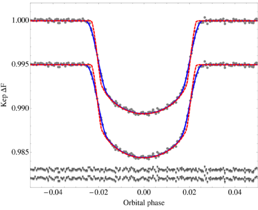
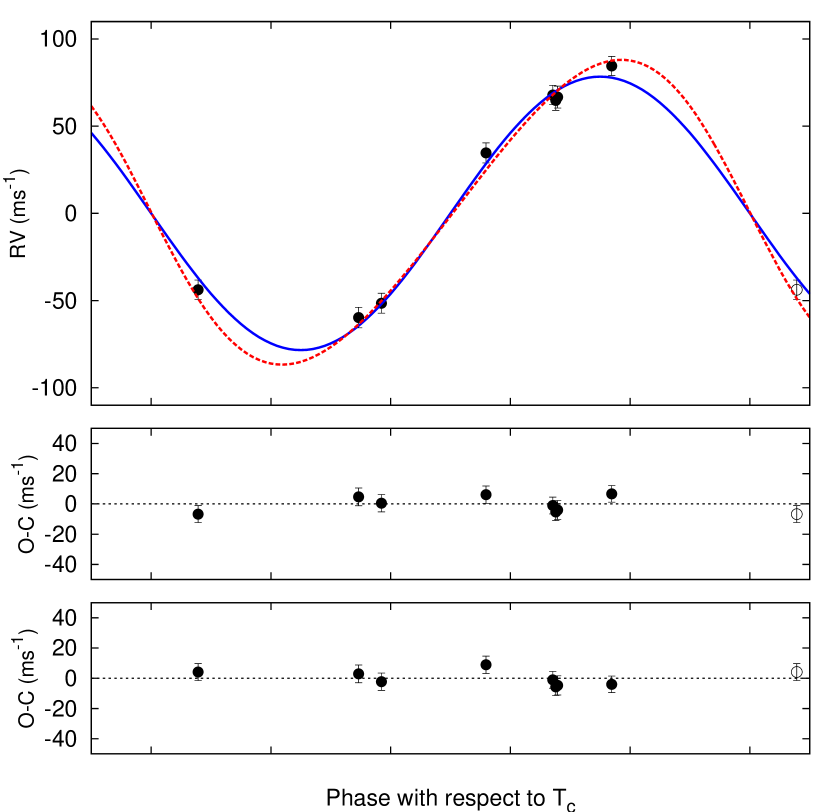
Kepler-6b was discovered by Dunham et al. (2010). In a similar manner to the other planets, we find consistent values for most parameters when compared to the Dunham et al. (2010) analysis. The fitted models on the phase-folded lightcurves for method B are shown on Figure 12. Correlated noise was checked for in the residuals using the Durbin-Watson statistic, which finds which is well within the 1% critical level of . The orbital fits to the RV points using method B are shown in Fig. 13, depicting both the circular and eccentric fits. The final planetary parameters are summarized at the bottom of Table 6.
6.1.2 Eccentricity
The global circular fit yields a and the eccentric fit obtains for the RVs. Based on an F-test, the inclusion of two new degrees of freedom to describe the eccentricity is justified with a significance of - The system is therefore best described with a circular orbit with the current observations. We constrain to 95% confidence.
6.1.3 Secondary eclipse
We here only consider the circular fit since the eccentric solution is not statistically significant. We find no evidence for a secondary eclipse detection for Kepler-6b. However, our analysis does exclude secondary eclipses of depth ppm or greater to 3- confidence, which excludes a geometric albedo to the same level. This therefore excludes the possibility of a planet covered in reflective clouds. A brightness temperature of K is ruled out to the same level, which places no constraints on the redistribution.
6.1.4 Properties of the parent star Kepler-6
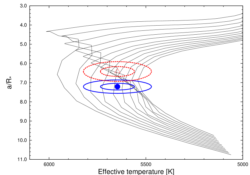
The Yonsei-Yale model isochrones from Yi et al. (2001) for metallicity = are plotted in Figure 14, with the final choice of effective temperature and marked, and encircled by the 1 and 2 confidence ellipsoids, both for the circular and the eccentric orbital solution. Here the MCMC distribution of comes from the global modeling of the data.
| Parameter | Discovery | Method A.c | Method A.e | Model B.c | Model B.e |
|---|---|---|---|---|---|
| Fitted params. | |||||
| /days | |||||
| (BJD-2,454,000) | |||||
| /s | - | ||||
| /s | - | ||||
| /s | - | ||||
| /% | - | ||||
| - | |||||
| /days-1 | - | ||||
| /ppm | - | ||||
| 0∗ | 0∗ | 0∗ | |||
| 0∗ | 0∗ | 0∗ | |||
| /ms-1 | |||||
| /ms-1 | |||||
| /ms-1day-1 | 0∗ | 0∗ | 0∗ | 0∗ | 0∗ |
| /days | 0∗ | 0∗ | 0∗ | 0∗ | |
| SME derived params. | |||||
| /K | |||||
| log | |||||
| (dex) | |||||
| () | |||||
| - | ∗ | ∗ | |||
| - | ∗ | ∗ | |||
| Model indep. params. | |||||
| /∘ | |||||
| 0∗ | 0∗ | 0∗ | |||
| /∘ | - | - | - | ||
| RV jitter () | - | 0.6 | 0.0 | ||
| /gcm-3 | |||||
| log | |||||
| /s | - | ||||
| /(BJD-2,454,000) | - | ||||
| Derived stellar params. | |||||
| log | |||||
| /mag | - | ||||
| Age/Gyr | |||||
| Distance/pc | - | ||||
| Derived planetary params. | |||||
| /gcm-3 | |||||
| /AU | |||||
6.2. Transit timing analysis
6.2.1 Analysis of variance
We find TTV residuals of 17.4 seconds and TDV residuals of 25.4 seconds. The TTV indicates timings consistent with a linear ephemeris, producing a of 7.8 for 11 degrees of freedom. The TDV is also consistent with a non-variable system exhibiting a of 11.4 for 12 degrees of freedom.
For the TTV, we note that for 11 degrees of freedom, excess scatter producing a of 28.5 would be detected to 3- confidence. This therefore excludes a short-period signal of r.m.s. amplitude seconds. Similarly, for the TDV, we exclude scatter producing a of 30.1, or a short-period r.m.s. amplitude of seconds, to 3- confidence. This constitutes a 0.53% variation in the transit duration.
These limits place constraints on the presence of perturbing planets, moons and Trojans. For the case a 2:1 mean-motion resonance perturbing planet, the libration period would be cycles and thus we do not possess sufficient baseline to look for such perturbers yet. However, a 4:3 resonance would produce a libration period of cycles and thus we would expect the effects to be visible over the 14 observed cycles so far. This therefore excludes a 4:3 resonant perturber of mass to 3- confidence.
The current TTV data rules out an exomoon at the maximum orbital radius (for retrograde revolution) of . The current TDV data rules an exomoon of at a minimum orbital distance.
Using the expressions of Ford & Holman (2007) and assuming , the expected libration period of Kepler-6b induced by Trojans at L4/L5 is 16.7 cycles and therefore we can search for such TTVs. We find such Trojans of cumulative mass at angular displacement are excluded by our timings. Inspection of the folded photometry at from the transit centre excludes Trojans of effective radius to 3- confidence.
6.2.2 Periodograms
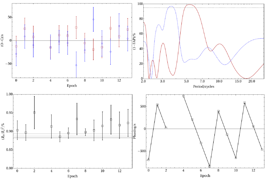
The TTV periodogram reveals a significant peak of period cycles with amplitude seconds and FAP 2.6-, which is one of our highest significances found, yet still below our formal detection threshold of 3-. Nevertheless, the signal warrants a more detailed investigation as it does not appear to land on any of the probable aliasing frequencies.
Given that Trojans should induce libration of period 16.7 cycles, this hypothesis can be instantly discounted. For two planets in a : mean motion-resonance, we may set the TTV signal’s period to be equal to the expression for the expected libration period (from Agol et al. (2005)) and solve for . This yields , or a period ratio of , which does not appear to be a resonant configuration. Barnes & Greenberg (2006) used the Hill criterion to provide an expression for estimating period ratios which are not guaranteed to be dynamically stable (equation 2). Using this expression, we estimate period ratios of and are unlikely to be stable for masses above . This makes the hypothesis of a mean-motion resonance unlikely.
For an out-of-resonant signal, the period of the TTV is more variable, depending on the difference between the perturber’s period and the nearest resonant position, quantified by the parameter in Agol et al. (2005). For a completely non-resonant system, and the period ratio is 6.34. As we move closer to resonance, this period ratio decreases. For the maximally non-resonant configuration, the perturber would require a mass of to generate the putative TTV signal. Given that this is approximately the same mass as the transiting planet and the period ratio is not large, it is clear that such a signal would be evident in the RV data. This makes the hypothesis of a non-resonant perturber unlikely but not completely excluded due to the possibility of out-of-the-plane perturbers (see Nesvorny & Beauge (2010); Veras et al. (2010)).
If such a signal was due to an aliasing of an exomoon’s orbital period, the maximum amplitude would occur for a moon at the maximum orbital separation given by Domingos et al. (2006), for a retrograde configuration. A moon of mass could generate such a signal and closer moons require larger masses. Such a moon should produce a photometric dip of between 40ppm and 170ppm, depending on its composition. Following the method outlined in Kipping (2009c), we may use the phasing predicted by the TTV fit to folded the individual transit residuals for cases where maximum planet-moon separation is predicted; epochs 1, 7 & 11 and the time-reversed epochs 4 & 9. Inspection of this folded residual rules out exomoons of to 2- confidence.
An additional method of confirming a moon would be through a TDV analysis. The TDV periodogram does have one significant peak at days though but with a weaker significance of - and amplitude seconds. Using the ratio of the TTV and TDV amplitude, Kipping (2009a) showed a solution for the exomoon period is possible. Following this method and assuming both the TTV peak and the TDV peak are genuinely due to a moon, we estimate an exomoon period of hours which would place the moon at a semi-major axis of planetary radii, i.e. within the planet’s volume. Although there is a large uncertainty on this, we conclude that the hypothesis of an exomoon inducing both the TTV and TDV putative signals is highly improbable.
The TDV peak is quite likely to be spurious due to the proximity of the periodogram peak to twice the Nyquist frequency. The exomoon hypothesis can be further interrogated by evaluating the range of dynamically stable moons around Kepler-6b. Assuming Jovian-like tidal dissipation values of and , the expression of Barnes & O’Brien (2002) indicate that a single moon could only be stable for the age of the system if it has a mass below . In contrast, the TTV could only be produced by moons suggesting we would require to make the two compatible. In conclusion, there is no confirming evidence for the moon hypothesis and at thus we cannot assign this explanation to the TTV peak.
The TTV signal’s period of 17.3 days is similar to that what we might expect for the star’s rotational period and thus could be due to the motion of star spots across the stellar surface, as observed by Alonso et al. (2008) for CoRoT-2b. Based upon the projected rotation of the star and the inferred stellar radius, we estimate the rotation period to be days which is compatible with the period of the TTV signal. A bisector analysis is not possible due to the very low cadence but will be possible once short-cadence data becomes available. We propose that this is the most likely explanation for the signal, based upon the current evidence.
The phasing signal has a period of 4 cycles, which is close to both periods found in the TTV and TDV periodograms. This therefore detracts credence to the hypothesis that these signals are genuine. Further observations, particularly in short-cadence mode, where phasing will not be a significant issue, will clarify the reality of these signals.
6.3. Depth and OOT Variations
The transit depth is consistent with the globally fitted value yielding a of 10.1 for 12 degrees of freedom. Similarly, the OOT levels are flat yielding a of 5.1 for 12 degrees of freedom.
| Epoch | /(BJD-2,454,000) | /s | /% | |
|---|---|---|---|---|
| 0 | ||||
| 1 | ||||
| 2 | ||||
| 3 | - | - | - | - |
| 4 | ||||
| 5 | ||||
| 6 | ||||
| 7 | ||||
| 8 | ||||
| 9 | ||||
| 10 | ||||
| 11 | ||||
| 12 | ||||
| 13 |
7. Kepler-7b
7.1. Global fits
7.1.1 Comparison to the discovery paper
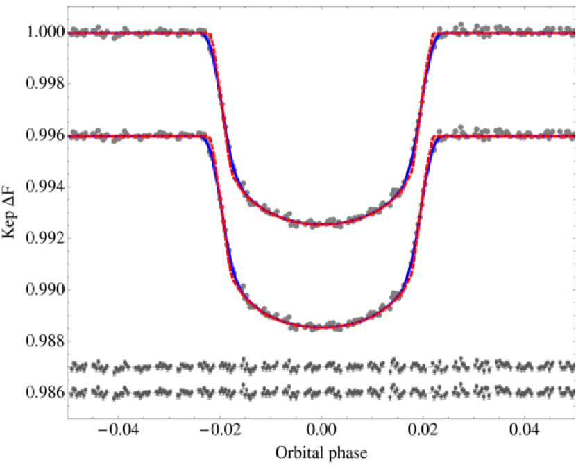
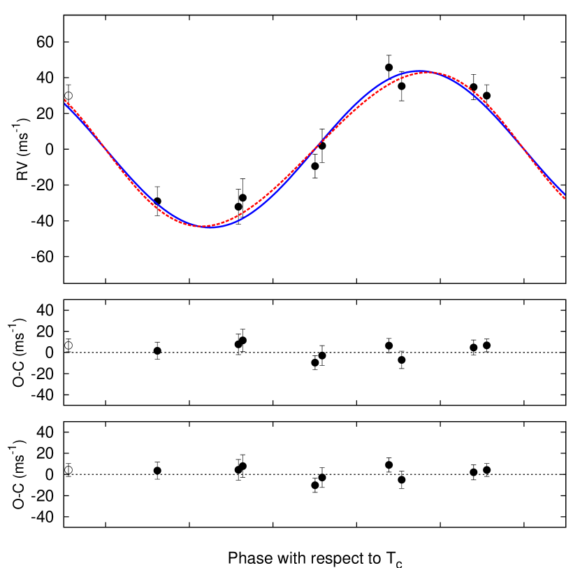
Kepler-7b was discovered by Latham et al. (2010). The planet is noteworthy for its very low density and thus significant inflation. Our global fits find highly consistent results with the original discovery paper. We note that the Latham et al. (2010) values are the most consistent with our own values out of any of discovery papers discussed in this work. The fitted models on the phase-folded lightcurves are shown on Figure 16 for method B. Correlated noise was checked for in the residuals using the Durbin-Watson statistic, which finds , at the border of the 1% critical level of , suggesting correlated noise is marginal. The orbital fits to the RV points are shown in Fig. 19, depicting both the circular and eccentric fits using method B. Unusually, both methods A and B found stellar jitter levels consistent with zero, which suggests the publicly available RV measurements have perhaps overestimated errors. The final planetary parameters are summarized at the bottom of Table 8.
7.1.2 Eccentricity
The global circular fit of method A yields a and the eccentric fit obtains for the RVs. An F-test finds that the eccentric fit has a significance of 79.4%. Therefore, we conclude that the eccentric fit does not meet our detection criteria and we constrain to 95% confidence.
One obvious question at this point is whether the range of allowed eccentricities could explain the bloated radius of Kepler-7b through tidal heating. The value of the planet is an element of large uncertainity here but we can constrain ’s minimum limit using the same method we adopted for Kepler-4b. We find that . One may argue that this is only valid under the assumption that the eccentric model is selected over the circular one, but we would counter that in the circular model case the tidal heating is zero anyway and thus the hypothesis of tidal heating being the origin of the bloated radius is invalid.
Using the posterior distribution of the minimum allowed value, we can translate this to a maximum allowed tidal energy dissipation using the expressions of Peale & Cassen (1978):
| (16) |
We divide this value by the amount of power hitting the planetary surface, found by to give us the posterior of the fraction of maximum allowed tidal heating relative to the incoming radiation and find . We therefore conclude that tidal heating plays a negligible role in the heating of Kepler-7b and the planet’s inflated radius.
7.1.3 Secondary eclipse
As before, method B is the better tool to constrain secondaries due to its rescaling method. Method B detects a secondary eclipse in the circular fits of depth ppm and significance 3.5- (99.96%). We note that Latham et al. (2010) reported a 2.4- weakly detected eclipse but did not report a depth estimate. The MCMC distribution of the values for method B is shown in Figure 18.
Inspection of the method A and Latham et al. (2010) values relative to the method B result reveals a clear difference and we must consider why we obtain such different numbers. All of the fits are circular and thus the orbital solutions are nearly identical with the eclipse occuring at the same phase in each case. The only difference between them is the definition of the out-of-eclipse baseline. Method A assumes the same baseline level for both primary and secondary transit whereas method B uses a simplified phase curve model as described in §2.2. If the secondary eclipse local baseline is different from the primary transit baseline, method A would move towards an average solution and actually attenuate the eclipse depth. The same attenuation also occurs in the Latham et al. (2010) which utilizes the same technique as method A (D. Latham, personal communication).
To investigate this futher, we may compare the three baseline levels found by method B: , and . The first two values are compatible with a constant but the baseline surrounding the secondary eclipse is clearly larger. If the secondary eclipse baseline is larger, method A would favor a lower average baseline due to and and thus find a lower secondary eclipse. This seems to be the explanation with method A finding . We believe this explains the discrepancy between the two methods.
Using the method B results only, the difference in baselines indicates a day-night contrast. Using our MCMC trials, we estimate a nightside flux ppm which is of 2.4- significance. We can also calculate the day-night difference explicitly and we find ppm. Since nightside flux cannot be due to reflected light, this supports the hypothesis of thermal emission as a source for both the secondary eclipse and the phase curve.
There is a very strong caveat to bear in mind for the day-night contrast. The data we have analyzed has been processed by the Kepler pipeline which involves numerous data manipulation processes. Time trends of very low amplitude and of time periods of days may be affected by this processing, with the most probable behaviour being that of a long-cut filter. As a result, a strong-day night contrast could be attenuated by the act of passing through this filter. It is therefore still possible that the day-night contrast is 100% (i.e. equal to the secondary eclipse depth) and thus the light we are seeing is reflected light, rather than thermal emission, but the phase curve is artificially distorted by the pipeline processing.
If the secondary eclipse was due to thermal emission, we may estimate the brightness temperature by integrating the Planck function of the planet over the Kepler response function, divided by that of the star. We repeat this for planetary brightness temperatures from 2000K to 3000K in 1K steps and calculate in each case. We find that a best-fit brightness temperature of K, which is much larger than the equilibrium temperature of K. Even the nightside flux of ppm would require a temperature for the nightside of K. These very large temperatures do not seem consistent with the energy budget of the planet, particularly as tidal heating has already been shown to offer a negligible contribution to the energy budget of this planet. From stellar irradiation only, the redistribution factor would have to be 7.48 to re-create the dayside eclipse, which is greater than the maximum physically permitted value of 8/3. The only remaining possibility is internal heating, for which we find a heat source responsible for 2440 K could explain both the dayside and nightside fluxes. This would require an internal heat source of , which is equivalent to the luminosity of an M6-M7 star. For example, LHS 292 (M6.5) and VB8 (M7) have luminosities of and respectively.
Whilst other sources of heating are possible apart from tidal, for example radioactivity, the magnitude required detracts credence from the hypothesis of thermal emission as the principal origin for the eclipse depth.
If due to reflection, method B finds a geometric albedo of , which is somewhat larger than the value found for Kepler-5b of , but not greatly different from the albedos of Jupiter and Saturn (0.52 and 0.47 respectively) and consistent with the study of Cowan & Agol (2010). We believe this latter hypothesis, as with Kepler-5b, is a more plausible scenario for the secondary eclipse measurement. As a consequence, we should not expect any nightside flux, which bears some questions on the apparent non-zero nightside flux detected in this study. There are two possible explanations which are consistent with reflection: i) the nightside flux is not statistically significant at 2.4- ii) the phase curve has been attenuated due to the Kepler pipeline producing effects which mimic a long-cut filter iii) is increased away from zero nightside flux due to the phase curve of the planet i.e. reflected light from the viewable crescent. In reality, a combination of these seems probable. Once more transits become available for analysis, a more sophisticated phase curve model can be fitted to the data set to resolve this question.


7.1.4 Properties of the parent star Kepler-7
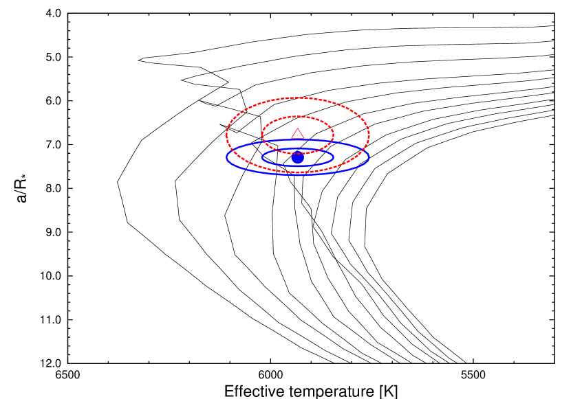
The Yonsei-Yale model isochrones from Yi et al. (2001) for metallicity = are plotted in Figure 20, with the final choice of effective temperature and marked, and encircled by the 1 and 2 confidence ellipsoids, both for the circular and the eccentric orbital solution. Here, the MCMC distribution of comes from the global modeling of the data.
| Parameter | Discovery | Method A.c | Method A.e | Model B.c | Model B.e |
|---|---|---|---|---|---|
| Fitted params. | |||||
| days | |||||
| (BJD-2,454,000) | |||||
| /s | - | ||||
| /s | - | ||||
| /s | - | ||||
| /% | - | ||||
| - | |||||
| /days-1 | - | ||||
| /ppm | - | ||||
| 0∗ | 0∗ | 0∗ | |||
| 0∗ | 0∗ | 0∗ | |||
| /ms-1 | |||||
| /ms-1 | 0 | ||||
| /ms-1day-1 | 0∗ | 0∗ | 0∗ | 0∗ | 0∗ |
| /days | 0∗ | 0∗ | 0∗ | 0∗ | 0∗ |
| SME derived params. | |||||
| /K | |||||
| log | |||||
| (dex) | |||||
| () | |||||
| - | ∗ | ∗ | |||
| - | ∗ | ∗ | |||
| Model indep. params. | |||||
| /∘ | |||||
| 0∗ | 0∗ | 0∗ | |||
| /∘ | - | - | - | ||
| RV jitter () | - | 0.0 | 0.0 | ||
| /gcm-3 | |||||
| log | |||||
| /s | - | ||||
| /(BJD-2,454,000) | - | ||||
| Derived stellar params. | |||||
| log | |||||
| /mag | - | ||||
| Age/Gyr | |||||
| Distance/pc | - | ||||
| Derived planetary params. | |||||
| /gcm-3 | |||||
| /AU | |||||
7.2. Transit timing analysis
7.2.1 Analysis of variance
We find TTV residuals of 32.1 seconds and TDV residuals of 22.2 seconds. The TTV indicates timings consistent with a linear ephemeris, producing a of 9.1 for 7 degrees of freedom (75.1% significance of excess). The TDV is also consistent with a non-variable system exhibiting a of 4.1 for 8 degrees of freedom (84.9% significance of being too low).
For the TTV, we note that for 7 degrees of freedom, excess scatter producing a of 21.8 would be detected to 3- confidence. This therefore excludes a short-period signal of r.m.s. amplitude seconds. Similarly, for the TDV, we exclude scatter producing a of 23.6, or a short-period r.m.s. amplitude of seconds, to 3- confidence. This consitutes a 0.50% variation in the transit duration.
These limits place constraints on the presence of perturbing planets, moons and Trojans. For the case a 2:1 mean-motion resonance perturbing planet, the libration period would be cycles and thus we do not possess sufficient baseline to look for such perturbers yet. After a further 102 cycles have been obtained at the same photometric quality, the presence of a 2:1 resonant perturber of mass may be constrained.
The current TTV data rules out an exomoon at the maximum orbital radius (for retrograde revolution) of . The current TDV data rules an exomoon of at a minimum orbital distance.
Using the expressions of Ford & Holman (2007) and assuming , the expected libration period of Kepler-7b induced by Trojans at L4/L5 is 21.4 cycles and therefore we do not yet possess sufficient baseline to search for these TTVs. Inspection of the folded photometry at from the transit centre excludes Trojans of effective radius to 3- confidence.
What is peculiar about this system is that the TTV produces a slight excess variance whilst the TDV does the opposite. The error on the TDV data points, and thus the scatter, should be exactly the same as the TTV points, or in fact slightly larger due to limb darkening effects. Thus, the observation of the TTV scatter being much larger than the TDV scatter is curious. We note for all other planets we studied we found the TDV scatter is greater than or equal to the TTV scatter. Also, for several planets we find the observed scatter is much lower than the uncertainties predict, suggesting we have overestimated our errors. If this is true for the Kepler-7b system, the TDV scatter indicates that the measurement uncertainties should be scaled by a factor of 0.71. This factor should be common to the TTV, which would change the observed from 9.1 to 17.7, for 7 degrees of freedom. The scaled would have a significance of 98.7%, or 2.5-, which is still below our formal detection threshold. Nevertheless, we identify Kepler-7b as an important target for continued transit timing analysis.
7.2.2 Periodograms
The TTV F-test periodogram presents one significant peak very close to Nyquist frequency, which we may discard. The TDV periodogram presents no significant peaks.
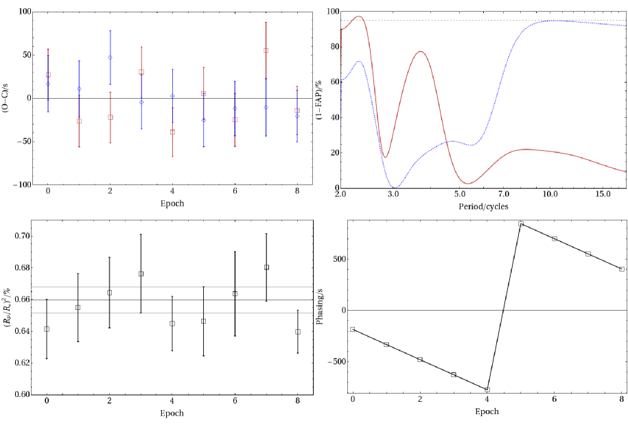
7.3. Depth and OOT Variations
The transit depth is consistent with the globally fitted value yielding a of 5.8 for 8 degrees of freedom. Similarly, the OOT levels are flat yielding a of 3.4 for 8 degrees of freedom.
| Epoch | /(BJD-2,454,000) | /s | ||
|---|---|---|---|---|
| 0 | ||||
| 1 | ||||
| 2 | ||||
| 3 | ||||
| 4 | ||||
| 5 | ||||
| 6 | ||||
| 7 | ||||
| 8 |
8. Kepler-8b
8.1. Global Fits
8.1.1 Comparison to the discovery paper
Kepler-8b was discovered by Jenkins et al. (2010a). Kepler-8b posed several unique problems not encountered with the other Kepler planets. The data format of the public data was quite different from the other sets. Typical values of the photometric data was whereas the other data sets where . This suggests that either the photometry was raw differential magnitudes or normalized fluxes with unity subtracted. We tried both assumptions and that the normalized fluxes minus unity assumption led to system parameters more consistent with the original discovery paper. This assumption has been since confirmed (personal communication with J. Jenkins).
Another peculiarity of the data is that the r.m.s. scatter is not constant but actually increases significantly with time, as discussed in §3.2. The source of this varying scatter is an instrumental effect, caused by oscillations in the photometry as a result of a heater on one of the two reaction wheel assemblies that modulates the focus by m (see Jenkins et al. (2010c) for more details). Since the discovery of this effect in the Q1 photometry, the Kepler Team have subsequently trimmed the bounding temperatures for this heater to reduce the amplitude and heater cycle (J. Jenkins, personal communication). Therefore, future data sets will not suffer from this effect as accutely as the photometry analyzed here. Concordantly, the results obtained in our analysis may not be as reliable as for the other Kepler planets.
In our analysis, we disregard radial velocity points occuring during the transit to avoid the Rossiter-McLaughlin effect. This is justified since our prinicpal goal here is to produce refined system parameters rather measure the spin-orbit alignment.
We find the orbit is consistent with a circular orbit and derive a significantly lower planetary mass than that reported by Jenkins et al. (2010a). The fitted models on the phase-folded lightcurves are shown on Figure 23. The orbital fits to the RV points are shown in Fig. 24, depicting both the circular and eccentric fits. The final planetary parameters are summarized at the bottom of Table 10.
The residuals of the lightcurve fits from method A (fitted limb darkening) were inspected using the Durbin-Watson statistic, which finds , indicating time correlated noise is certainly present. The origin of this is very likely the heater oscillations described earlier. An F-test periodogram finds the largest peak occuring at 3.27 hours with amplitude 50.6 ppm, significance 4.25-. The rich forest of perdiodic lines make a correction unfeasible, as seen in Figure 23.
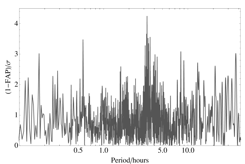
8.1.2 Eccentricity
The global circular fit yields a and the eccentric fit obtains . Based on an F-test, the inclusion of two new degrees of freedom to describe the eccentricity is justified at a significance of 13.1% and thus is not accepted.
8.1.3 Secondary eclipse
Using the circular fit, there is no evidence for a secondary eclipse; we can exclude secondary eclipses of depth ppm to 3- confidence, or equivalently geometric albedos . We can also exclude a brightness temperature K to the same confidence level, which places no constraints on the redistribution of heat around the planet.
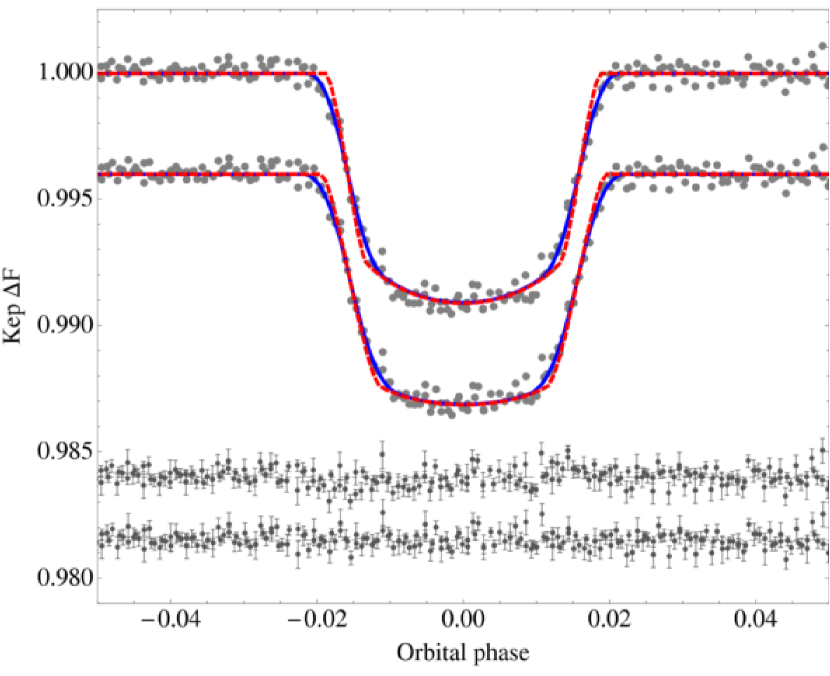
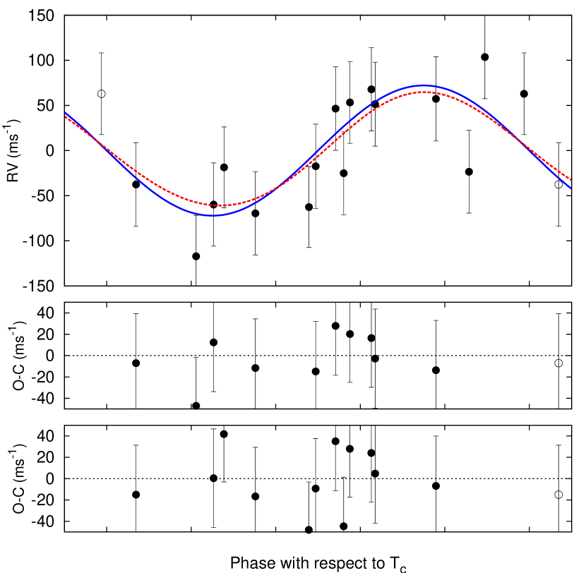
8.1.4 Properties of the parent star Kepler-8
The Yonsei-Yale model isochrones from Yi et al. (2001) for metallicity = are plotted in Figure 25, with the final choice of effective temperature and marked, and encircled by the 1 and 2 confidence ellipsoids, both for the circular and the eccentric orbital solution. Here the MCMC distribution of comes from the global modeling of the data.
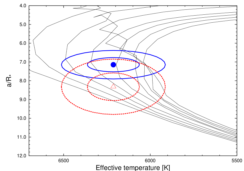
| Parameter | Discovery | Method A.c | Method A.e | Model B.c | Model B.e |
|---|---|---|---|---|---|
| Fitted params. | |||||
| days | |||||
| (BJD-2,454,000) | |||||
| /s | - | ||||
| /s | - | ||||
| /s | - | ||||
| /% | - | ||||
| - | |||||
| /days-1 | - | ||||
| /ppm | - | - | |||
| 0∗ | 0∗ | 0∗ | |||
| 0∗ | 0∗ | 0∗ | |||
| /ms-1 | |||||
| /ms-1 | |||||
| /ms-1day-1 | 0∗ | 0∗ | 0∗ | 0∗ | 0∗ |
| /days | 0∗ | 0∗ | 0∗ | 0∗ | 0∗ |
| 1∗ | |||||
| SME derived params. | |||||
| /K | |||||
| log | |||||
| (dex) | |||||
| () | |||||
| - | ∗ | ∗ | |||
| - | ∗ | ∗ | |||
| Model indep. params. | |||||
| /∘ | |||||
| 0∗ | 0∗ | 0∗ | |||
| /∘ | - | - | - | ||
| RV jitter () | - | 19.7 | 20.7 | ||
| /gcm-3 | |||||
| log | |||||
| /s | - | ||||
| /(BJD-2,454,000) | - | ||||
| Derived stellar params. | |||||
| log | |||||
| /mag | |||||
| Age/Gyr | |||||
| Distance/pc | |||||
| Derived planetary params. | |||||
| /gcm-3 | |||||
| /AU | |||||
8.2. Transit timing analysis
8.2.1 Analysis of variance
We find TTV residuals of 68.1 seconds and TDV residuals of 92.2 seconds. The TTV indicates timings consistent with a linear ephemeris, producing a of 10.7 for 11 degrees of freedom. The TDV is also consistent with a non-variable system exhibiting a of 18.8 for 12 degrees of freedom (84.9% significance of excess).
For the TTV, we note that for 11 degrees of freedom, excess scatter producing a of 28.5 would be detected to 3- confidence. This therefore excludes a short-period signal of r.m.s. amplitude seconds. Similarly, for the TDV, we exclude scatter producing a of 30.1, or a short-period r.m.s. amplitude of seconds, to 3- confidence. This consitutes a 1.46% variation in the transit duration.
These limits place constraints on the presence of perturbing planets, moons and Trojans. For a 2:1 mean-motion resonance, the libration period would be cycles and thus we do not possess sufficient baseline yet to look for such perturbers. However, a 4:3 resonance system would yield a libration period of cycles and therefore we would expect to see such a signal with the 13 cycles observed. This means a 4:3 perturber of is ruled out to - confidence by the current TTV data for this object. After 83 cycles have been obtained at the same photometric quality, the presence of a 2:1 resonant perturber of mass may be constrained.
The current TTV data rules out an exomoon at the maximum orbital radius (for retrograde revolution) of . The current TDV data rules an exomoon of at a minimum orbital distance.
Using the expressions of Ford & Holman (2007) and assuming , the expected libration period of Kepler-8b induced by Trojans at L4/L5 is 25.5 cycles and therefore we do not yet possess sufficient baseline to search for these TTVs. Inspection of the folded photometry at from the transit centre excludes Trojans of effective radius to 3- confidence.
8.2.2 Periodograms
The TTV periodogram reveals a peak at twice the Nyquist period, which we disregard. No other significant peaks are present. The TDV also has no significant peaks. The phasing signal appears to have a period of 2 cycles.
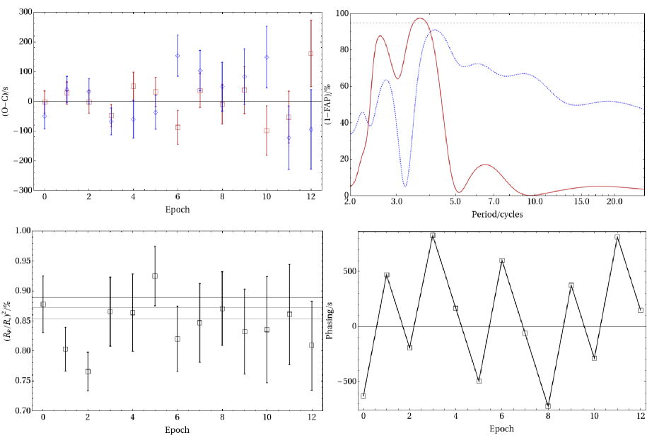
8.3. Depth and OOT Variations
The transit depth produces a slightly excess scatter in reference to the global fit. We find a of 18.0 for 12 degrees of freedom, which is 1.6- significant. The OOT is consistent with the global value yielding for 12 degrees of freedom. As for the TDV, the varying depths are neither statistically significant nor particularly robust in light of the irregularities encountered with this data set.
| Epoch | /(BJD-2,454,000) | /s | ||
|---|---|---|---|---|
| 0 | ||||
| 1 | ||||
| 2 | ||||
| 3 | ||||
| 4 | ||||
| 5 | ||||
| 6 | ||||
| 7 | ||||
| 8 | ||||
| 9 | ||||
| 10 | ||||
| 11 | ||||
| 12 |
9. Discussion
Due to the large number of results presented in this paper, we will here summarize the key findings not available in the original discovery papers:
-
Secondary eclipse of Kepler-7b is detected to 3.5- confidence with depth ppm, indicative of a geometric albedo of .
-
A marginally significant orbital eccentricity is detected for the Neptune-mass planet Kepler-4b to 2- confidence, with an eccentricity of .
-
A marginally significant (1.8-) secondary eclipse is detected for Kepler-5b with a depth of ppm, for which the most plausible explanation is reflected light due to a geometric albedo of .
-
A 2.6- significance peak in the TTV periodogram of Kepler-6b is detected, which is not easily explained as an alias frequency. Perturbing planets and exomoons are unlikely to be responsible either and currently our favored hypothesis is one of stellar rotation.
-
We derive significantly different impact parameters for all of the Kepler planets except Kepler-7b.
9.1. Comparison of three hot-Neptunes
The eccentricity of Kepler-4b is marginally detected to 2- confidence. If confirmed, this would mean that three of the four hot-Neptunes discovered through the transit method have eccentricities around 0.15-0.20, the other two being GJ 436b and HAT-P-11b. HAT-P-26b is the fourth transiting hot-Neptune, recently discovered by hartman:2010 and this system also possesses a marginal eccentricity of . With HAT-P-26b possessing a FAP of 12% and Kepler-4b being 11.8%, it would seem likely that at least one of these two systems is genuinely eccentric.
In all cases, the tidal circularization time is expected to be much lower than the age of the system for Jovian-like tidal dissipation values, which raises the question as to why these planets still retain eccentric orbits. Generally two hypotheses have been put forward: i) an unseen perturbing planet pumps the eccentricity of the hot Neptune ii) hot Neptunes have larger values than expected.
At the time when only one example of an eccentric Neptune was known, GJ 436b, Ribas et al. (2008) made the reasonable deduction that is was more likely an unseen perturber was present. However, given that three such planets are now known, Occam’s razor seems to favor the alternative hypothesis. For all three hot-Neptunes to have perturbing planets which all remain hidden from detection and yet produce nearly identical eccentricity pumping levels appears to be a less likely scenario than that of a common solution due to intrinsically different tidal dissipation values and formation history. For Kepler-4b, the observed eccentricity indicates if no eccentricity pumping is occurring.
We also point out that the physical properties of Kepler-4b differ greatly between the eccentric and circular fits (see Table 12), due to the large impact of eccentricity on the lightcurve derived stellar density (Kipping, 2010a). Further RV measurements are likely required to resolve the eccentricity of this system, since an occultation is generally not expected to be observable given the very low .
| Planet | Mass/ | Radius/ | Density/gcm-3 | logcgs) | e | /K |
| GJ 436b | ||||||
| HAT-P-11b | ||||||
| Kepler-4b (circ) | ||||||
| Kepler-4b (ecc) | ||||||
| Neptune | 9.6 | |||||
| Uranus | 12.1 | |||||
| Saturn | 26.0 |
9.2. Secondary eclipses
We detect a secondary eclipse for the bloated Kepler-7b of depth ppm and 3.5- confidence. This is above our formal detection threshold of 3- thus represents an unambiguous detection. Thermal emission is an unlikely source for the eclipse since the depth indicates a brightness temperature of K, which is far in excess of the equilibrium temperature of the planet of K. A geometric albedo of offers a more plausible explanation for this eclipse depth. However, we do note that a significant nightside flux is apparently present which is not consistent with the reflection hypothesis. We believe that this nightside flux is likely an artifact of the Kepler pipeline whose effects may mimic a long-cut filter. Although Kepler-7b exhibits similarities to HD 209458b in terms of its very low density, the albedo clearly marks the planet at distinct given that for HD 209458b (Rowe et al., 2008). The study of Burrows et al. (2008) seems to indicate that the albedo requires the presence of reflective clouds, possibly composed of iron and/or silicates, as seen in L-dwarf atmospheres. It is interesting to note that Kepler-7 is times more metal-rich than HD 209458, and the planet has a higher equilibrium temperature of K than that of HD 209458b with K.
We also note that, to our knowledge and if confirmed, the above measurement is the first determination of a transiting planet’s albedo at visible wavelengths, and thus the first detection the associated reflected light. This compliments the recent polarimetric detection of reflected light of HD 189733b was made by Berdyugina et al. (2008), and recently confirmed in Berdyugina et al. (2011). Visible secondary eclipses of other planets have been made for HAT-P-7b (Borucki et al., 2009) and CoRoT-1b (Snellen et al., 2009) but in both cases the eclipse can be explained through a combination of reflected light plus thermal emission or even simply pure thermal emission for models of large day-night contrasts, which is in fact expected for these extremely hot-Jupiters (Fortney et al., 2008). In contrast, thermal emission cannot explain the Kepler-7b secondary eclipse unless the planet has an internal heat source with a luminosity equivalent to that of a M6.5 dwarf star, which is highly improbable.
We also find weak significance of a secondary eclipse for Kepler-5b of 2- confidence. Further transits will either confirm or reject this hypothesis but we note that the obtained depth is quite reasonable for this planet. Whilst thermal emission again seems unlikely based upon the required temperature of 2500 K versus the equilibrium temperature of 1800 K, a geometric albedo of offers a satisfactory explanation for the eclipse.
For Kepler-6b and Kepler-7b, we find no evidence of a secondary eclipse, but the measurements do constrain the geometric albedos to and at 3- confidence. For Kepler-4b, the measurement place no constraints on the geometric albedo.
9.3. Differences with the discovery papers
For almost all cases, we find significantly different impact parameters from the discovery papers, but self-consistent between methods A and B. There are also several examples of other parameters being different. These can be easily reviewed by consulting Tables 2, 4, 6, 8 and 10. For example, for Kepler-4b, we find a very low stellar density implying a larger stellar radius and thus larger planetary radius. Other examples of differing parameters include the eccentricity and secondary eclipse parameters already discussed.
9.4. On the error budget of planetary parameters
The exquisite lightcurves measured by Kepler lead to very low uncertainties on certain parameters, even in the long-cadence mode. One example is the fitted ratio-of-radii , where the error is about 0.5% (e.g., for Kepler-7b). The median error for the first 70 known transiting exoplanets (TEPs) on is 0.9%, about double that of Kepler-7b. Limiting factors on the precision of this purely geometrical factor are the limb-darkening values for the Kepler bandpass and the slight degeneracy with other parameters that are affected by the long-cadence binning, even if re-sampled models are fitted (such as the impact parameter). Using short-cadence data, deriving precise limb-darkening coefficients, and accumulating many transits will significantly improve errors in .
The typical errors on the period for the first five Kepler planets are days, about 6 times greater than the median error of the period of the first 70 published TEPs, or about 20-times the error quoted in e.g. Hartman et al. (2009) for HAT-P-12b, an example of a TEP discovery using photometry data spanning 2 years. This error on the Kepler planet periods, however, comes from a dataset with short time-span (44 days), while the ground-based results come from multi-year campaigns. The median error on the ephemeris () for the current 5 Kepler planets is days, about half that of the known TEPs ( days). Precision of the ephemeris data will greatly improve during the lifetime of the Kepler mission just by accumulating more data, and switching to short-cadence mode.
At first glance perhaps somewhat surprisingly, the errors on the Kepler planetary masses and radii are not different from the rest of the transiting exoplanet population. The typical error on planetary masses for 70 transiting exoplanets is , whereas the error for radii is . In our analysis the errors for planetary masses and radii for Kepler planets have roughly the same values.
There are multiple reasons behind this. Planetary mass and radius scale with the respective parameters of the host star. In our analysis, and are determined from stellar isochrones, using , and . Each of these quantities have significant errors. The stellar and come from SME analysis of the spectra, which, in turn, due to the faintness of the Kepler targets, are of low S/N, and have larger than usual errors. The other input parameter, , is related to the lightcurve parameters , , and the RV parameters and . While is quite precise for the Kepler transits (median error 0.02 as compared to 0.15 for the known TEPs), the impact parameter from the current LC Kepler data-set have errors comparable to ground-based transits. The main limiting factor, however, are the and Lagrangian orbital parameters from the RV data. Due to the faintness of the targets, the orbital fits have considerable errors in and . As a result, the error on for the current Kepler data in this work (median error 0.26) is similar to that of the known TEPs (median error 0.2). This effect is well visible on the isochrone figures (Fig. 4, 10, 14, 20, 25), where the 1- and 2- confidence ellipses are shown for all Kepler planets for both the circular and eccentric solutions, with the latter clearly covering a much larger area on the isochrones. Finally, the error in the planetary mass also scales with the RV semi-amplitude, which has typical errors for the Kepler planets similar to the median error of the known planets ( ). Given the faintness of the Kepler targets this is an impressive result.
A breakthrough in both accuracy and precision of and can be expected from exploiting the extraordinary precision of Kepler, and nailing down the stellar parameters via asteroseismology (see Mulet-Marquis et al. (2009), Christensen-Dalsgaard et al. (2010)). Alternatively (or simultaneously), if parallaxes for the Kepler targets become available (possibly from the Kepler data), then analyses similar to that performed for HAT-P-11b (Bakos et al., 2009) can be performed, where the “luminosity-indicator” in the isochrone fitting will be the absolute magnitude of the stars, as opposed to the constraint. A final possibility is a dynamical measurement of the stellar mass by measuring the transit timing variations of two TEPs within the same system (Agol et al., 2005).
9.5. Transit timing with LC data
After the discovery of an exoplanet in Kepler’s field, the subsequent photometry is switched to short-cadence (SC) mode. It was generally expected that this would be the only way to produce meaningful TTV studies. However, we have found that by carefully correcting for the long integration time, the long-cadence (LC) photometry yields transit times consistent with a linear ephemeris and of r.m.s. scatters of 10-20 seconds are possible.
Despite the evident timing precision possible with the LC photometry, some issues require further investigation. The effect of phasing, as defined in §2.3.4 remains somewhat unclear but in numerous instances we find that peaks in the TTV and TDV periodograms occur near to the phasing period. Subsequent aliasing and frequency mixing also seems to lead to numerous false positives in the periodograms and these issues may be diminished by using SC data, but are unlikely to completely disappear.
Out of all of the studied planets, we found only one peak in the timing periodograms which does not appear spurious. Kepler-6b exhibits a 2.6- peak of period days and amplitude seconds. We investigated the plausibility of this signal being a perturbing planet or exomoon but found no convincing supporting evidence, although such hypotheses could not excluded. Our favored hypothesis is that of stellar rotation inducing such a signal, as reported by Alonso et al. (2008) for CoRoT-2b. The host star has a rotational period of days and thus it is consistent with the TTV period. A bisector analysis, as performed by Alonso et al. (2008), is not possible for this data due to the long cadence. However, the SC data will be able to either confirm or reject this hypothesis.
Finally, we note that the uncertainties in all of the parameters from individual fits show evidence for being overestimates, based upon the observed scatter of these parameters between various transits. Both methods employed in this analysis found very similar errors and thus the reason for consistent overestimation of the errors remains unclear. Both methods employed Markov Chain Monte Carlo (MCMC) techniques for obtaining these errors, which may be linked to the overestimation. If the MCMC trials are unable to sample the true global minimum, perhaps due to slightly erroneous limb darkening coefficients or insufficient numerical resolution in the integration time compensation procedure, the errors are expected to be overestimated. Nevertheless, in searching for evidence of signals, the accurate estimation of error bars is just as important as the best-fit value. We have proposed a F-test periodogram which is insensitive to absolute errors, only their relative weightings, and also penalizes overly-complex models. Further detailed investigation with future Kepler timings will be possible and should shed light on this issue.
9.6. Constraints on planets, moons & Trojans
We find no convincing evidence for perturbing planets, moons or Trojans in any of the systems studied here. We are able to exclude the presence of mean-motion resonant (MMR) planets for Kepler-5b, Kepler-6b and Kepler-8b of masses , and respectively, to 3- confidence. The corresponding resonant configurations are period ratios of 3:2, 4:3 and 4:3. We do not yet possess sufficient temporal baseline to investigate MMR planets for Kepler-4b and Kepler-7b.
Extrasolar moons at a maximum orbital separation are excluded by the TTV measurements for Kepler-4b through to Kepler-8b of masses , , , and respectively, to 3- confidence. Extrasolar moons at a minimum orbital separation are excluded by the TDV measurements of masses , , , and respectively, to 3- confidence.
For Kepler-4b, Kepler-7b and Kepler-8b, we do not yet possess sufficient temporal baseline to search for Trojans through TTV measurements. However, for Kepler-5b and Kepler-6b we are able to exclude Trojans of angular displacement from L4/L5 of cumulative mass and respectively, to 3- confidence. For all five planets, we can inspect the photometry at from the transit center for signs of a photometric dip due the occultation of the host star by the Trojans. This search yielded no detections but does exclude Trojans of effective radii , , , and for the five planets sequentially, to 3- confidence.
References
- Adams & Laughlin (2006) Adams, F. C. & Laughlin, G., 2006, ApJ, 649, 1004
- Agol et al. (2005) Agol, E., Steffen, J., Sari, R., & Clarkson, W. 2005, MNRAS, 359, 567
- Alonso et al. (2008) Alonso, R., Aigrain, S., Pont, F., Mazeh, T. et al., 2008, arXiv:0807:4828
- Bakos et al. (2007) Bakos, G. Á., et al. 2007b, ApJ, 670, 826
- Bakos et al. (2009) Bakos, G. Á., et al. 2009, arXiv:0901.0282
- Baraffe et al. (2008) Baraffe, I., Chabrier, G., & Barman, T. 2008, A&A, 482, 315
- Barnes & O’Brien (2002) Barnes, J. W. & O’Brien, D. P., 2002, ApJ, 575, 1087
- Barnes & Greenberg (2006) Barnes, R. & Greenberg, R., 2006, ApJL, 647, 163
- Beaulieu et al. (2010) Beaulieu, J. P. et al., 2010, MNRAS, accepted
- Berdyugina et al. (2008) Berdyugina, S. V., Berdyugin, A. V., Fluri, D. M. & Piirola, V., 2008, ApJ, 673, L83
- Berdyugina et al. (2011) Berdyugina, S. V., Berdyugin, A. V., Fluri, D. M. & Piirola, V., 2011, ApJL, accepted (astro-ph:1101.0059)
- Borucki et al. (2009) Borucki, W. J. et al., Science, 325, 709
- Borucki et al. (2010a) Borucki, W. J. et al., Science, 327, 977
- Borucki et al. (2010b) Borucki, W. J. et al., ApJL, 713, 126
- Burrows et al. (2008) Burrows, A., Ibgui, L. & Hubeny, I., 2008, ApJ, 682, 1277
- Carpenter (2001) Carpenter, J. M. 2001, AJ, 121, 2851
- Carter et al. (2008) Carter, J. A., Yee, J. C., Eastman, J., Gaudi, B. S. & Winn, J. N., 2008, ApJ, 689, 499
- Christensen-Dalsgaard et al. (2010) Christensen-Dalsgaard, J., Kjeldsen, H., Brown, T. M., Gilliland, R. L., Arentoft, T., Frandsen, S., Quirion, P.-O., Borucki, W. J., Koch, D. & Jenkins, J. M., ApJ, 713, 164
- Claret (2000) Claret A., 2000, A&A, 363, 1081
- Cowan & Agol (2010) Cowan, N. & Agol, E. 2010, submitted to ApJ
- Deming et al. (2005) Deming, D., Seager, S., Richardson, L. J. & Harrington, J. 2005, Nature, 434, 740
- Deming et al. (2007) Deming, D., Harrington, J., Laughlin, G., Seager, S., Navarro, S. B., Bowman, W. C., & Horning, K. 2007, ApJ, 667, L199
- Díaz-Cordovés et al. (1995) Díaz-Cordovés, J., Claret, A., & Giménez, A., 1995, A&AS, 110, 329
- Domingos et al. (2006) Domingos, R. C., Winter, O. C. & Yokoyama, T. 2006, MNRAS, 373, 1227
- Dunham et al. (2010) Dunham, E. et al., 2010, ApJL, 713, 136
- Eastman et al. (2010) Eastman, J., Siverd, R., Gaudi, B. S., 2010, PASP, submitted
- Ford (2006) Ford, E. 2006, ApJ, 642, 505
- Ford & Holman (2007) Ford, E. B. & Holman, M. J., 2007, ApJ, 664, 51
- Fortney et al. (2008) Fortney, J. J., Lodders, K., Marley, M. S., & Freedman, R. S. 2008, ApJ, 678, 1419
- Gauss (1816) Gauss, C. F., 1816, Zeitschrift für Astronomie und verwandt Wissenschaften, 1, 187
- Gelman & Rubin (1992) Gelman, A. & Rubin, D. B., 1992, Statistical Science, 7, 457
- Gibson et al. (2009) Gibson, N. P. et al., 2009, ApJ, 700, 1078
- Gillon et al. (2007) Gillon, M., et al. 2007, A&A, 472, L13
- Hartman et al. (2009) Hartman, J. D., 2009, ApJ, 706, 785
- Hellier et al. (2009) Hellier, C. H. et al., 2009, Nature, 460, 1098
- Holman & Murray (2005) Holman, M. J., & Murray, N. W. 2005, Science, 307, 1288
- Jenkins et al. (2010a) Jenkins, J. et al., 2010, ApJ, 724, 1108
- Jenkins et al. (2010b) Jenkins, J. et al., 2010, ApJL, 13, 87
- Jenkins et al. (2010c) Jenkins, J. et al., 2010, ApJL, 713, L120
- Kipping (2008) Kipping, D. M., 2008, MNRAS, 389, 1383
- Kipping (2009a) Kipping, D. M., 2009, MNRAS, 392, 181
- Kipping (2009b) Kipping, D. M., 2009, MNRAS, 396, 1797
- Kipping (2009c) Kipping, D. M., Fossey, S. J., Campanella, G., Schneider, J. & Tinetti, G., 2009, Proceedings of Pathways Towards Habitable Planets
- Kipping (2010a) Kipping, D. M., 2010, MNRAS, accepted, arXiv: 1004.3819
- Kipping (2010b) Kipping, D. M., 2010, MNRAS, accepted, arXiv: 1004.3741
- Kipping & Tinetti (2010) Kipping, D. M. & Tinetti, G., 2010, MNRAS, submitted
- Knutson et al. (2007) Knutson, H. A., Charbonneau, D., Allen, L. E., Fortney, J. J., Agol, E., Cowan, N. B., Showman, A. P., Cooper, C. S. & Megeath, S. T., 2007 Nature, 447, 183
- Koch et al. (2010) Koch, D. et al., 2010, ApJL, 713, 131
- Kurucz (2006) Kurucz R., 2006, Stellar Model and Associated Spectra (http://kurucz.harvard.edu/grids.html)
- Latham et al. (2010) Latham, D. et al., 2010, ApJL, 713, 140
- Liddle (2007) Liddle, A. 2007, MNRAS, 377, 74
- Mulet-Marquis et al. (2009) Mulet-Marquis, C., Baraffe, I., Aigrain, S. & Pont, F., 2009, A&A, 506, 153
- Pál et al. (2008a) Pál, A., et al. 2008, ApJ, 680, 1450
- Pál (2008b) Pál, A. 2008, MNRAS, 390, 281
- Pál (2009) Pál, A. 2009, MNRAS, 396, 1737
- Pál (2009b) Pál, A., 2009, arXiv:0906.3486 PhD thesis
- Peale & Cassen (1978) Peale, S. J. & Cassen, P., 1978, Icarus, 36, 245
- Press et al. (1992) Press, W. H., Teukolsky, S. A., Vetterling, W. T. & Flannery, B. P., 1992, Numerical Recipes in C: the art of scientific computing, Second Edition, Cambridge University Press
- Lucy & Sweeney (1971) Lucy, L. B. & Sweeney, M. A. 1971, AJ, 76, 544
- Mandel & Agol (2002) Mandel, K., & Agol, E. 2002, ApJ, 580, L171
- Mandushev et al. (2007) Mandushev, G., et al. 2007, ApJ, 667, L195
- Nesvorny & Beauge (2010) Nesvorny, D. & Beauge, C. 2010, ApJ, 709, 44
- Ribas et al. (2008) Ribas, I., Font-Ribera, A., & Beaulieu, J.-P. 2008, ApJ, 677, L59
- Rowe et al. (2008) Rowe, J. F., et al., 2008, ApJ, 689, 1345
- Sartoretti & Schneider (1999) Sartoretti, P. & Schneider, J., 1999, A&AS, 14, 550
- Schwarz (1978) Schwarz, G. 1978, Ann. Statist., 5, 461
- Skrutskie et al. (2006) Skrutskie, M. F., et al. 2006, AJ, 131, 1163
- Skumanich (1972) Skumanich, A. 1972, ApJ, 171, 565
- Snellen et al. (2009) Snellen, I. A. G., de Mooij, E. J. W. & Albrecht, S., 2009, Nature, 459, 543
- Tegmark et al. (2004) Tegmark, M., et al. 2004, Phys. Rev. D, 69, 103501
- Tingley & Sackett (2005) Tingley, B. & Sackett, P. D., 2005, ApJ, 676, 1011 (TS05)
- Torres (2008) Torres, G., 2008, ApJ, 671, L65
- Yi et al. (2001) Yi, S. K. et al. 2001, ApJS, 136, 417
- Veras et al. (2010) Veras, D., Ford, E. B. & Payne, M. J. 2010, submitted to ApJ (astro-ph:1011.1466)
- Welsh et al. (2010) Welsh, W. F., Orosz, J. A., Seager, S., Fortney, J. J., Jenkins, J., Rowe, J. F., Koch, D., Borucki, W. J., 2010, ApJ, 713, L145
| Parameter | Name | Definition |
|---|---|---|
| Linear limb darkening coefficient | Linear term of the quadratic description of the stellar limb darkening | |
| Quadratic limb darkening coefficient | Quadratic term of the quadratic description of the stellar limb darkening | |
| Mid companion-star separation | Companion-star separation in units of stellar radii at the approximate moment of mid-transit | |
| Companion-star separation | Companion-star separation in units of the stellar radius | |
| Eccentricity | Orbital eccentricity of the companion’s orbit | |
| Argument of pericentre | Argument of pericentre of the companion’s orbit | |
| Period | Orbital period of the companion | |
| Ratio-of-radii | Ratio of the companion’s radius to the stellar radius () | |
| Radius of the companion | Radius of the companion | |
| Radius of the host star | Radius of the host star | |
| Impact parameter | Approximate value of when ; also given by | |
| Sky-projected separation | Sky-projected separation of the companion’s centre | |
| and the host star’s centre in units of stellar radii | ||
| Inclination | Orbital inclination of the companion’s orbit relative to the line-of-sight of the observer | |
| Semi-major axis | Semi-major axis of the companion’s orbit in units of the stellar radius | |
| Semi-major axis | Semi-major axis of the companion’s orbit | |
| Epoch of mid-transit | Mid-transit time of the first transit in the sequence | |
| Mid-transit time | Mid-transit time for a given epoch | |
| Lagrange parameter | ||
| Lagrange parameter | ||
| Transit duration | Time for companion to move across the stellar disc with entry | |
| First contact | Instant when and | |
| Second contact | Instant when and | |
| Mid-transit time | Instant when i.e. inferior conjunction | |
| Third contact | Instant when and | |
| Fourth contact | Instant when and | |
| Total duration | Time for companion to move between contact points I and IV | |
| Full duration | Time for companion to move between contact points II and III | |
| Ingress duration | Time for companion to move between contact points 1 and 2 | |
| Egress duration | Time for companion to move between contact points 3 and 4 | |
| Total eclipse duration | Analogous to but for the secondary eclipse | |
| Ingress/Egress duration | For circular orbits, | |
| duration | Approximate expression for from Kipping (2010a) | |
| Stellar density | Average density of the host star | |
| Zeta over | The reciprocal of one half of the transit duration using the Tingley & Sackett (2005) approximation. | |
| Upsilon over | The reciprocal of one half of the transit duration using the Kipping (2010a) approximation | |
| Primary flux | Constant flux term for primary-portion of phase curve | |
| Secondary flux | Constant flux term for secondary-portion of phase curve | |
| Middle flux | Constant flux term for middle-portion of phase curve | |
| Observed flux | Flux observed by the instrument as a function of time | |
| Model flux | Flux from a given model as a function of time | |
| Stellar flux | Flux received from the star | |
| Day-side flux | Flux received from the day-side of the planet | |
| Relative dayside flux | Ratio of flux emitted from dayside of planet to stellar flux | |
| Relative nightside flux | Ratio of flux emitted from nightside of planet to stellar flux | |
| Transit model flux | Model flux for the primary transit | |
| Secondary model flux | Model flux for secondary eclipse | |
| Blending factor | Parameter to quantify amount of blended light in the aperture | |
| Phase function | Flux received from planet+star+blend without transits or eclipses | |
| RV offset | Constant used for offsetting the radial velocity measurements | |
| RV semi-amplitude | Semi-amplitude of the radial velocity signal | |
| Effective temperature | Effective temperature of the star | |
| Metallicity | Metallicity of the host star | |
| Projected rotation velocity | Projected stellar rotation velocity | |
| Stellar mass | Mass of the host star | |
| Planetary mass | Mass of the planet | |
| Luminosity | Stellar luminosity | |
| Absolute magnitude | Absolute magnitude of the host star | |
| planetary density | Density of the planet | |
| Stellar surface gravity | Surface gravity of the host star | |
| Planetary surface gravity | Surface gravity of the planet | |
| Equilibrium temperature | Equilibrium temperature of the planet | |
| Circularization timescale | Time for eccentricity to reduce by an e-fold | |
| Quality factor of planet | Quality factor of planet due to tidal dissipation |
| Model | Circular Orbit BICs | Eccentric Orbit BICs |
|---|---|---|
| Kepler-4 | ||
| Free ; Free | 34.395 | 36.354 |
| Free ; Fixed | 31.144 | 33.300 |
| Fixed ; Free | 31.486 | 35.732 |
| Fixed ; Fixed | 29.556 | 32.685 |
| Kepler-5 | ||
| Free ; Free | 29.275 | 29.222 |
| Free ; Fixed | 26.768 | 28.487 |
| Fixed ; Free | 43.990 | 47.592 |
| Fixed ; Fixed | 45.321 | 45.889 |
| Kepler-6 | ||
| Free ; Free | 17.467 | 19.790 |
| Free ; Fixed | 21.234 | 17.693 |
| Fixed ; Free | 15.592 | 17.878 |
| Fixed ; Fixed | 20.157 | 16.834 |
| Kepler-7 | ||
| Free ; Free | 13.195 | 17.276 |
| Free ; Fixed | 13.0113 | 15.518 |
| Fixed ; Free | 11.508 | 15.530 |
| Fixed ; Fixed | 11.160 | 13.664 |
| Kepler-8 | ||
| Free ; Free | 30.877 | 37.213 |
| Free ; Fixed | 28.162 | 34.311 |
| Fixed ; Free | 28.163 | 34.340 |
| Fixed ; Fixed | 27.130 | 31.675 |
| (BJD-2454900) | Standard deviations | (BJD-2454900) | Standard deviations |
| Kepler-4 | |||
| 73.176 | 3.5 | 93.590 | 5.3 |
| 84.660 | -5.1 | 96.982 | -3.7 |
| Kepler-5 | |||
| 55.418 | 3.9 | 53.641 | 4.1 |
| 62.795 | 5.3 | 54.437 | 9.6 |
| 70.683 | 4.3 | 71.030 | -3.8 |
| 77.753 | 3.7 | ||
| Kepler-6 | |||
| 61.733 | 4.1 | 56.236 | 4.1 |
| 67.945 | -3.5 | 66.024 | 3.6 |
| 86.070 | 3.9 | 88.011 | 4.2 |
| 55.929 | 3.5 | 94.775 | 4.0 |
| Kepler-7 | |||
| 72.113 | -3.6 | 84.415 | -3.5 |
| 96.287 | -3.9 | 94.571 | 3.6 |
| Kepler-8 | |||
| 78.192 | 10.1 | 56.656 | 3.7 |
| 58.883 | 17.3 | 58.781 | 4.2 |
| 60.681 | 4.1 | 73.349 | 3.7 |
| 53.039 | 4.7 |