THE VARIATION OF RELATIVE MAGNETIC HELICITY AROUND MAJOR FLARES

Abstract

We have investigated the variation of magnetic helicity over a span of several days around the times of 11 X-class flares which occurred in seven active regions (NOAA 9672, 10030, 10314, 10486, 10564, 10696, and 10720) using the magnetograms taken by the Michelson Doppler Imager (MDI) on board the $Solar$ $and$ $Heliospheric$ $Observatory$ ($SOHO$). As a major result we found that each of these major flares was preceded by a significant helicity accumulation, (1.8–16)$\times$10⁴² Mx² over a long period (0.5 to a few days). Another finding is that the helicity accumulates at a nearly constant rate, (4.5–48)$\times$10⁴⁰ Mx² hr^-1, and then becomes nearly constant before the flares. This led us to distinguish the helicity variation into two phases: a phase of monotonically increasing helicity and the following phase of relatively constant helicity. As expected, the amount of helicity accumulated shows a modest correlation with time-integrated soft X-ray flux during flares. However, the average helicity change rate in the first phase shows even stronger correlation with the time-integrated soft X-ray flux. We discuss the physical implications of this result and the possibility that this characteristic helicity variation pattern can be used as an early warning sign for solar eruptions.

1 INTRODUCTION

Magnetic helicity is a measure of twists, kinks, and inter-linkages of magnetic field lines (Berger & Field 1984) and has been an important parameter in solar dynamo theories (Parker 1955). While the source of the magnetic helicity lies below the surface of the Sun, it was recently recognized as a useful parameter in describing solar features observed above surface such as spiral patterns of sunspot fibrils, helical patterns in filaments and coronal mass ejections (CMEs; for a review, see Brown et al. 1999). Naturally magnetic helicity studies have been directed to the energy buildup and instability leading to eruptions and CMEs (e.g., Rust 2001; Kusano et al. 2004; Phillips et al. 2005). More recently, several studies were carried out to relate the change of magnetic helicity to the problem of impending or triggering solar flares. Moon et al. (2002a) studied the magnetic helicity change around major flares to find its rapid helicity change before flares, and concluded that a sudden helicity injection may trigger flares. Moon et al. (2002b) applied the same approach to seven homologous flares in the active region, NOAA 8100, over a period of 6.5 hr to find a good correlation between the amount of incremental helicity and the soft X-ray flux during each homologous flare. The results from both studies thus point to the idea that the helicity change occurring over short timescales (around a half hour) can be a significant factor in triggering flares. Kusano et al. (2003) proposed annihilation of magnetic helicity as a triggering mechanism for solar flares. Numerical simulations were carried, which show that, if the helicity is sharply reversed within a magnetic arcade, reconnection quickly grows in the helicity inversion layer, driving explosive dynamics. Yokoyama et al. (2003) studied flare activities in active region NOAA 8100 to find that most of the flare events occurred about half a day after the helicity injection rate changed its sign, and the positions of H$\alpha$ emission in flares well correspond to the helicity inversion lines in space. Sakurai & Hagino (2003) studied two active regions appeared in 2001 (NOAA 9415 and 9661), both of which have produced X-class flares. Their finding was, on the contrary, that the magnetic helicity integrated over the regions evolved slowly and did not show abrupt changes at the time of the flares, although the distributions of magnetic helicity changed significantly over a few days in the regions.

In this paper, we study long term (a few days) variations of the magnetic helicity around major X-class flares. While some of the above studies suggest short-term helicity change as an important topic for flare triggering, Hartkorn & Wang (2004) found that the rapid helicity change at the time of a flare can occur as an artifact under the influence of flare emission on the spectral line adopted in MDI measurements. This means that a short term variation during strong flares can hardly be measured with enough accuracy. However we can study a long-term variation of the magnetic helicity with active region magnetograms gathered over many days excluding the times of flares. Our research is therefore focused on a possible characteristic helicity evolution pattern that is associated with flare impending mechanisms.

2 CALCULATION OF MAGNETIC HELICITY

By magnetic helicity, we refer to the relative magnetic helicity in the rest of this paper, i.e., the helicity relative to that of the potential field state. With the time-dependent measurement of longitudinal magnetic fields in the photosphere, we can only approximately determine the change rate of the relative magnetic helicity (Demoulin & Berger 2003). We further use a simplified expression for the helicity change rate (Chae 2001) given by

$$\left(\frac{dH_{r}}{dt}\right)_{LCT}=-\int_{s}2({\bf{A}}_{p}\cdot{\bf{v}}_{LCT})B_{n}dS$$ (1)

where $B_{n}$ is the normal component of the magnetic field; ${\bf A}_{p}$ is the vector potential of the potential field; ${\bf v}_{LCT}$ represents the apparent horizontal motion of field lines; $dS$ is the surface integral element and the integration is over the entire area of the target active region. Although this expression does not explicitly include the helicity change by the vertical motion of field lines (see Kusano et al. 2002), Démoulin & Berger (2003) pointed out that it actually accommodates both the vertical and horizontal motions of flux tubes as far as no flux tube newly emerges from or totally submerges into the surface. As we will show later in presenting the result of helicity calculation, this requirement is not always met.

We determine the quantities in the above equation using full disk MDI (Scherrer et al. 1995) magnetograms following the procedure described in Chae & Jeong (2005). First, we approximately determine $B_{n}$ from the line-of-sight magnetic field $B_{l}$ in the MDI magnetograms, simply considering the projection effect, i.e., $B_{l}=B_{n}\cos\psi$ where $\psi$ is the heliocentric angle of the point of interest, assuming that the magnetic field on the solar photosphere is normal to the solar surface. Second, ${\bf A}_{p}$ is calculated from $B_{n}$ by using the Fast Fourier Transform method as usual. The extent of the spatial domain of the Fourier transform is taken about twice wider than the active region area in order to minimize the artifacts arising from the periodic boundary condition in the fast Fourier transform (Alissandrakis 1981). Third, ${\bf v}_{LCT}$ is calculated using the local correlation tracking (LCT) technique (November & Simon 1988). For local correlation tracking, we align all magnetograms in each event to the first image of the data set after correcting the differential rotation. We set the FWHM of the apodizing window function to 10″ and the time interval between two frames to 60 minutes, and performed LCT for all pixels with an absolute flux density greater than 5 G. Only the pixels with cross correlation above 0.9 are considered.

In selecting data we found that use of 1 minute cadence full-disk MDI (Scherrer et al. 1995) magnetograms is adequate for our purpose of investigating the long-term helicity evolution. However, there are occasionally found data gaps in the 60 minute cadence data set in which case we supplement the data gaps with 96 minute MDI magnetograms. The time interval of the supplemented data set is therefore not longer than 96 minute. To reduce the effect of the geometrical projection, we selected the active regions lying within 60% of the solar radius from the apparent disk center. Note that we use only full disk MDI magnetograms that have 2″$\times$2″ pixel size. Therefore the LCT velocities calculated here may have been systematically underestimated compared with the LCT velocities calculated with the higher resolution (0.6″$\times$0.6″) MDI data (Longcope et al. 2007).

After the helicity change rate is determined as a function of time, we integrate it with respect to time to determine the amount of helicity accumulation:

$$\Delta H=\int_{t_{0}}^{t}\left(\frac{dH_{r}}{dt}\right)dt$$ (2)

where $t_{0}$ and $t$ are the start and end time of the helicity accumulation, respectively. If $t_{0}$ is a time when the magnetic field is in the potential state, $\Delta H$ is simply the helicity, $H(t)$, at time $t$. However, there is no guarantee that we can observe, by chance, an active region in the potential energy state. We therefore set $t_{0}$ as the earliest time without significant helicity accumulation at which the average value of the helicity change rate over four hours is less than our nominal threshold in helicity change rate, 1$\times$10⁴⁰ Mx² hr^-1. If that time cannot be determined, we define $t_{0}$ as the time when the data set starts or when the previously accumulated helicity is released by a flare. The exact time of $t_{0}$ here is unimportant because it is only a trial value. After determining $H(t)$, we redefine $t_{0}$ as the time when the resulting helicity starts to increase from a nearly constant value.

3 Magnetic Helicity Variation

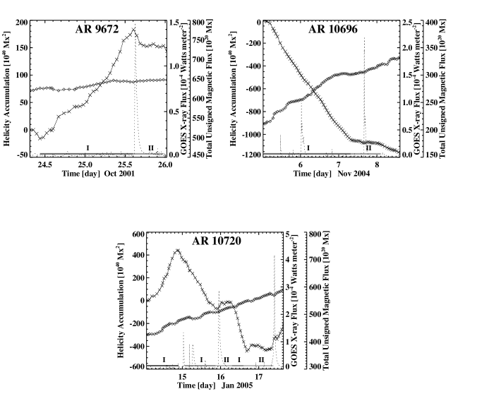
Figure 1: Time variations of helicity accumulation, magnetic flux, and $GOES$ X-ray flux for three active regions. The helicity is shown as cross symbols and the magnetic flux is shown as diamonds. The $GOES$ X-ray flux is shown as the dotted lines. Phase I, the interval over which the helicity accumulation is considered, and phase II, the following phase of relatively constant helicity, are marked.

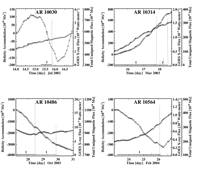
Figure 2: Same as in Fig. 1, but for additional events.

We present the helicity variation calculated for seven active regions in Figures 1 and 2. In both figures we plot the magnetic helicity accumulation together with the GOES soft X-ray light curve and magnetic flux as functions of time. The soft X-ray light curve is shown to indicate the flare times and the magnetic flux is shown to check the above-mentioned requirement for the approximation made in Equation (1). Note that the fluxes shown in this paper are total unsigned magnetic flux, i.e., sum of the absolute amounts of positive and negative fluxes, because net magnetic flux may show little change despite significant flux change in each polarity.

For the events shown in Figure 1 we can see that the helicity accumulates at a monotonic rate of change about 0.5–2 days before the flare onset, and then becomes almost constant before the flares. For convenience, we distinguish the magnetic helicity variation in two stages: a phase of monotonically increasing helicity (phase I) and the following phase of relatively constant helicity (phase II). This pattern is obvious for the four flares (2001 October 25, 2004 November 7, and 2005 January 16 and 17). For the 2005 January 15 event, the helicity increased up to 22:00 UT on January 14 and then decreased afterward. In this case, we do not consider that the flare occurred in phase II. It is then noted that these flares took place after a significant amount, $\sim$(1.8–11)$\times$10⁴² Mx², of helicity accumulation.

In Figure 2, we show the result for the other four active regions. Like the events in Figure 1, these flares also occurred after a significant helicity accumulation, $\sim$(1.9–16)$\times$10⁴² Mx². However, they occurred in the middle of the continuous helicity accumulation, unlike those events shown in Figure 1. In other word, the flares in Figure 2 occurred in phase I, while those in Figure 1 occurred in phase II. One common trend is, however, that all the events are apparently associated with a considerable amount of helicity build-up before the flares, whether they occurred in phase I or in phase II. In case where flares occur in phase II, it may imply that solar active regions can wait for major flares after the helicity accumulated to some limiting amount. This is seemingly contrary to the general belief that a flare occurs as soon as the system reaches some threshold. An active region may evolve to a certain stage where the helicity no longer increases, and the system waits until it unleashes the stored energy by producing flares due to certain mechanism of triggering.

Since we claimed that these large flares are always preceded by significant accumulation of helicity, as a reference we check the corresponding helicity variation in non-flaring times. We show such data in Figure 3. For all active regions under investigation, the amount of helicity change during nonflaring periods (Fig. 3) is much less than that around the major flare time. This convinces us that the above monotonically increasing helicity before major flares is a process associated with the flares and is not occurring in nonflare times. Another point to note in Figure 3 is that not only the helicity but also the total unsigned magnetic flux changes much less during the nonflaring time compared with the period before major flares. This implies that the increase of the magnetic helicity before major flares is, in part, related to the simultaneous increase of total unsigned magnetic flux.

It is also worthwhile to mention how the characteristic pattern of the helicity variation found here will depend on the sign of helicity. In our result obtained for seven active regions, similar amounts of both of positive and negative helicity were accumulated continuously and simultaneously during the whole time. It is therefore unlikely that counting the helicity in one and the other polarity separately yields a significantly different conclusion. On the other hand, some studies suggested that the sign-reversal of the helicity injection rate is important for flare activity and we need to compared them with the present result. Kusano et al. (2003) emphasized spatially sharp reversal of helicity sign triggers magnetic reconnection based on model simulation. While the model prediction is interesting and compelling, we excluded from the outset (see §1) the rapid helicity change during the flare time due to observational limitation. Our conclusion is valid only for the long term variation of helicity. Yokoyama et al. (2003) have found that flares tend to occur after reversal of helicity injection rate changed its sign. Although this is occasionally seen in our samples, (i.e., in the case of AR 10030 and AR 10720) as well, it is not always the case and we are unsure whether this is a necessary condition for the flares. More often than not, the helicity either remains constant or increases in one sign when the flare occurs.

4 Correlation with Soft X-ray Flux

We compare the helicity change rate, $dH/dt$ and accumulation amount, $\Delta H$ with the time integrated soft X-ray flux taken as the proxy for the flare energy release. In addition we check the helicity accumulation time, $\tau$, defined as the time interval of helicity accumulation measured from $t_{0}$ and the first coming flare. Prior to make such a comparison, the range of uncertainty of each quantity needs to be known. In general it is hard to trace all the possible uncertainties involved with each quantities in Equation (1). Fortunately, our targeted quantity given by Equation (2) involves integration in space and time and the uncertainty in each measured quantity is not propagating, but rather may cancel out in the process of spatial and time integration if it is random in nature. We thus focus the uncertainty estimate only on the linear approximation of the helicity variation that we are after. We first find out the best-fit linear function to the points $\Delta H(t_{i})$ lying in phase I (i.e., $t_{0}\leq t_{i}\leq t_{0}+\tau$) in the form of $F(t)=a(t-t_{0})+F(t_{0})$. Next we calculate the standard deviation, $\sigma$, of the scatter points with respect to this linear function, and plot two additional lines corresponding to the $\pm\sigma$ levels of the scatter points. Finally, we read the $y$-axis offsets of these two lines to determine $\sigma_{\Delta H}$ and the x-axis offsets to determine $\sigma_{\tau}$, respectively. In addition, we calculate the uncertainty of the slope $a$ itself in the form of $(\Delta H-\sigma_{\Delta H})/(\tau+\sigma_{\tau})\leq a\leq(\Delta H+\sigma_{\Delta H})/(\tau-\sigma_{\tau})$. The center value of $a$ here is taken as the average helicity change rate in the rest of this paper. Therefore, by the average helicity change rate, we do not mean the average of the quantities given in Equation (1), but we refer to the best fit slope to the helicity variation (eq. [2]) in phase I. The uncertainties shown in Figure 4 and Table 1 are those associated with our linear function fit only.

In Figure 4, we plot, as symbols, the helicity parameters against the GOES soft X-ray fluxes integrated over the flaring time ($F_{X}$, hereafter). Each symbol is identified with the event ID number in the figure together with uncertainty range represented by the bar (see also Table I). The solid lines show the least-squares linear fits to the data points. The correlation coefficients (CCs) of the linear fits are also given in each panel. Figure 4$a$ shows that there is a fairly good correlation (CC=0.86) between the helicity change rate and $F_{X}$. The amount of helicity accumulation also shows a modest correlation with $F_{X}$ (CC=0.68) as shown in Figure 4$b$, although not as good as for the helicity change rate. On the other hand, the correlation between helicity accumulation time $\tau$ and the soft X-ray flux is very poor with a weak tendency that the longer accumulation time $\tau$, the weaker soft X-ray flux $F_{X}$ (Fig. 4$c$).

We initially expected, on a general basis, that the helicity change $\Delta H$ would strongly correlate with $F_{X}$. It is therefore puzzling why the helicity change rate $dH/dt$ shows even a better correlation with $F_{X}$ in Figure 4. As a possibility, we considered that $\tau$ may be a factor in complicating the relationship between $\Delta H$ and $F_{X}$. A intriguing idea is that the magnetic energy decays much faster than the magnetic helicity in the presence of magnetic diffusion (Berger 1999). We thus compare $\Delta H$ with $\tau$ in Figure 4d, which unfortunately shows no obvious correlation between them. The small number of events used in this study is another restriction for finding a trend here. With the present result alone, it is fair to presume that the weaker correlation between $F_{X}$ and $\Delta H$ may arise from our inaccurate determination of the helicity accumulation amount due to unknown initial time of helicity build-up.

5 SUMMARY

We have investigated the variation of magnetic helicity over a time span of several days around the times of 11 X-class flares which occurred in seven active regions using MDI magnetograms to find the following results.

First, a substantial amount of helicity accumulation is found before the flare in all the events. The helicity increases at a nearly constant rate, (4.5–48)$\times$10⁴⁰ Mx² hr^-1, over a period of 0.6 to a few days, resulting in total amount of helicity accumulation in the range of (1.8–16)$\times$10⁴² Mx². Such a wide range of helicity accumulation indicates that each active region has its own limit of helicity storage to keep a stable magnetic structure in the corona. The finding of a monotonically increasing phase is similar to the earlier one by Sakurai & Hagino (2003) that the magnetic helicity integrated over the regions evolved slowly and did not show abrupt changes at the time of the flares. The helicity increase over days before the flares reconfirms the conventional idea that helicity accumulation by a certain amount is necessary for a large flare to occur (Kusano et al. 1995; Choe & Lee 1996).

Second, there is a strong positive correlation between the average helicity change rate of phase I and the corresponding GOES X-ray flux integrated over the flaring time. The amount of helicity accumulation during phase I also correlates with the soft X-ray flux, as expected, but the correlation is stronger with the helicity change rate. This result probably implies that the helicity change rate is more accurately determined than the amount of helicity change itself as the initial time of helicity build-up is poorly determined.

If the above correlations hold for a large number of events, we may predict the flare strength (the integrated X-ray flux) based on the helicity change rate. Monitoring of helicity variation in target active regions may also aid the forecasting of flares. A warning sign of flares can be given by the presence of a phase of monotonically increasing helicity, as we found that all the major flares occur after significant helicity accumulation. As a reference we have checked helicity variation of the six active regions in non-flaring times to find much lower helicity change rates compared with those around the major flares. We thus conclude that the relative magnetic helicity can be a powerful tool for predicting major flares.

Table 1: List of flares, helicity and accumulation time

ID	Flares	AR	Peak time	$F_{X}\tablenotemark{a}$	$|$$dH/dt$$|$	$|$$\Delta H$$|$	$\tau\tablenotemark{d}$
		number	$(UT)$	$(10^{-1}J/m^{2})$	$(10^{40}Mx^{2}hr^{-1})$	$(10^{42}Mx^{2})$	$(hr)$
1	X 1.3 on Oct 25, 2001	9672	15:02	2.3	6.2$\pm$0.9	1.8$\pm$0.1	29$\pm$2
2	X 3.0 on Jul 15, 2002	0030	20:08	1.4	13.3$\pm$1.5	1.9$\pm$0.1	14$\pm$1
3	X 1.5 on Mar 17, 2003	0314	19:05	1.3	6.4$\pm$1.6	3.9$\pm$0.5	63$\pm$8
4	X 1.5 on Mar 18, 2003	0314	12:08	1.3	13.3$\pm$1.4	2.3$\pm$0.1	17$\pm$1
5	X 18 on Oct 28, 2003	0486	11:10	20.0	48.4$\pm$6.3	14.5$\pm$0.9	30$\pm$2
6	X 10 on Oct 29, 2003	0486	20:49	9.1	46.8$\pm$3.0	15.9$\pm$0.5	34$\pm$1
7	X 1.2 on Feb 26, 2004	0564	02:03	0.75	4.5$\pm$0.4	3.1$\pm$0.1	70$\pm$3
8	X 2.2 on Nov 07, 2004	0696	16:06	2.1	19.8$\pm$0.7	10.7$\pm$0.2	54$\pm$1
9	X 1.3 on Jan 15, 2005	0720	00:43	1.3	22.2$\pm$4.1	4.2$\pm$0.4	19$\pm$2
10	X 2.8 on Jan 15, 2005	0720	23:00	6.6	22.5$\pm$1.2	4.3$\pm$0.1	19$\pm$1
11	X 4.1 on Jan 17, 2005	0720	09:52	9.1	40.8$\pm$5.5	3.2$\pm$0.2	8$\pm$1

Figure 3: Time variations of helicity accumulation, and magnetic flux for six nonflare active regions. The helicity is shown as crosses, and the magnetic flux is shown as diamonds.

Figure 4: Helicity parameters with $GOES$ X-ray flux integrated over the flaring time. Correlations of the integrated soft X-ray flux with ($a$) average helicity change rate of phase I, ($b$) the amount of helicity accumulation during phase I, and ($c$) helicity accumulation time. Correlation coefficient (CC) is specified in each panel. In ($d$), the amount of helicity accumulation is plotted as a function of the accumulation time. The uncertainties of the average helicity change rate, the amount of helicity accumulation, and the helicity accumulation time are shown as error bars in each panel.

References

- Alissandrakis (1981) Alissandrakis, C. E. 1981, A&A, 100, 197
- Berger & Field (1984) Berger, M. A., & Field, G. B. 1984, J. Fluid Mech., 147, 133
- Berger (1999) Berger, M. A. 1999, in M. R. Brown, R. C. Canfield, and A. A. Pevtsov (eds.) Magnetic Helicity in Space and Laboratory Plasmas, Geophys. Monogr., 111, 11
- Brown, Canfield, and Pevtsov (1999) Brown, M. R., Canfield, R. C., & Pevtsov, A. A. (eds.) 1999, Magnetic Helicity in Space and Laboratory Plasmas, Geophys. Monogr., 111
- Chae (2001) Chae, J. 2001, ApJ, 560, L95
- Chae & Jeong (2005) Chae, J., & Jeong, H. 2005, J. Korean Astron. Soc., 38, 295
- Choe & Lee (1996) Choe, G. S., & Lee, L. C. 1996, ApJ, 472, 372
- Démoulin & Berger (2003) Démoulin, P., & Berger, M. A. 2003, Sol. Phys., 215, 203
- Hartkorn & Wang (2004) Hartkorn, K., & Wang, H. 2004, Sol. Phys., 225, 311
- Kusano et al. (1995) Kusano, K., Suzuki, Y., & Nishikawa, K. 1995, ApJ, 441, 942
- Kusano et al. (2002) Kusano, K., Maeshiro, T., Yokoyama, T., & Sakurai, T. 2002, ApJ, 577, 501
- Kusano et al. (2003) Kusano, K., Yokoyama, T., Maeshiro, T., & Sakurai, T. 2003, Adv. Space Res., 32, 1931
- Kusano et al. (2004) Kusano, K., Maeshiro, T., Yokoyama, T., & Sakurai, T. 2004, ApJ, 610, 537
- Longcope et al. (2007) Longcope, D. W., Ravindra, B., & Barnes, G. 2007, ApJ, 668, 571
- Moon et al. (2002a) Moon, Y.-J., Chae, J., Wang, H., & Park, Y. D. 2002a, ApJ, 580, 528
- Moon et al. (2002b) Moon, Y.-J., Chae, J., Choe, G. S., Wang, H., Park, Y. D., Yun, H. S., Yurchyshyn, V., & Goode, P. R. 2002b, ApJ, 574, 1066
- November & Simon (1988) November, L. J., & Simon, G. W. 1988, ApJ, 333, 427
- Parker (1955) Parker, E. N. 1955, ApJ, 122, 293
- Phillips et al. (2005) Phillips, A. D., MacNeice, P. J., & Antiochos, S. K. 2005, ApJ, 624, L129
- Rust (2001) Rust, D. M. 2001, J. Geophys. Res., 106, 25075
- Sakurai & Hagino (2003) Sakurai, T., & Hagino, M. 2003, Adv. Space Res., 32, 1943
- Scherrer et al. (1995) Scherrer, P. H., et al. 1995, Sol. Phys., 162, 129
- Yokoyama et al. (2003) Yokoyama, T., Kusano, K., Maeshiro, T., & Sakurai, T. 2003, Adv. Space Res., 32, 1949