Robust Parameter Selection for Parallel Tempering

Abstract

This paper describes an algorithm for selecting parameter values (e.g. temperature values) at which to measure equilibrium properties with Parallel Tempering Monte Carlo simulation. Simple approaches to choosing parameter values can lead to poor equilibration of the simulation, especially for Ising spin systems that undergo $1^{s}t$-order phase transitions. However, starting from an initial set of parameter values, the careful, iterative respacing of these values based on results with the previous set of values greatly improves equilibration. Example spin systems presented here appear in the context of Quantum Monte Carlo.

1 Introduction

This paper describes our experience with and modifications to an algorithm to enhance Parallel Tempering (PT) Monte Carlo [1] known as Feedback Optimized Parallel Tempering (FOPT) [3]. Though our experimental analysis will focus on the Quantum Ising Spin Glass in a transverse field, we shall try to keep the concepts as general as possible as we believe that workers in as diverse fields as Bayesian Statistics, Computer Science, and Molecular Simulation may be interested in optimizing PT on difficult problems. While PT has proved itself to be an indispensable tool in computer simulation, certain aspects of some problems can present serious obstacles to its use. The idea of FOPT is to try to eliminate the barriers in replica-diffusion space that can hinder the decorrelative effect that PT is supposed to overcome. Our initial experiments with PT on the Quantum Ising Glass encountered precisely such difficulties, but we found it necessary to make some adaptations to FOPT for it to function robustly.

To ease the presentation to those unfamiliar with Quantum Monte Carlo (QMC) or spin systems but knowledgeable with Markov Chain Monte Carlo (MCMC, also called dynamical Monte Carlo) simulation, the specialized, physics-oriented concepts are confined to Section 4, which briefly reviews the Quantum Ising Glass and how it is simulated. Uninterested readers can skip that section and simply imagine that within is derived a set of intractable high-dimensional distributions (which in this case are defined over a binary-valued state space) that we wish to sample from.

Section 2 reviews the ideas of PT and FOPT; our contributions to improving the method are discussed in Section 3. Section 4, as mentioned above, discusses quantum spin simulation, and Section 5 presents some numerical data.

2 Parallel Tempering

2.1 Basic PT

An excellent general survey of PT can be found in [2]; for completeness some basic concepts are presented. Suppose we have a family $\{f_{k}(\mathbf{x})\}$ of $M$ distributions defined on a state space $\mathcal{X}$ each member of which is dependent on some parameter $\lambda_{k}$, i.e. $f_{k}(\mathbf{x})=f(\mathbf{x}|\lambda_{k})$. We assume that the terminal parameters $\lambda_{1}$ and $\lambda_{M}$ are fixed and that implementing naive MCMC at those values, for example local-variable Metropolis or Gibbs (heat bath) sampling, will result in slowly and quickly equilibrating (“mixing”) Markov Chains respectively. $\lambda_{1}$ and $\lambda_{M}$ could, for instance, be low and high temperatures; in the systems we simulate, $\lambda$ is a parameter that plays roughly the same role as temperature. The values of the remaining $\{\lambda_{k}\}$ are assumed to be flexible in this work provided that equilibration gets easier for increasing $k$. We refer to a local MCMC simulation at a given parameter value as a chain.

The method of PT supplements the usual within-system Monte Carlo updates with phases during which swaps of entire states between chains at different parameter values are attempted. A particular state is sometimes called a replica. In practice, to have a non-negligible swapping probability, exchanges are only attempted between neighboring parameters $\{\lambda_{k},\lambda_{k+1}\}$. An exchange is accepted probabilistically according to the Metropolis ratio

$$\alpha=\min\bigg{(}1,\frac{f_{k}(\mathbf{x}_{k+1})f_{k+1}(\mathbf{x}_{k})}{f_{k}(\mathbf{x}_{k})f_{k+1}(\mathbf{x}_{k+1})}\bigg{)}$$ (1)

It can be shown that the combination of the local MCMC moves and the swapping implements a Markov chain on the joint state space $\mathcal{X}^{M}$ whose invariant distribution is $f_{1}(\mathbf{x}_{1})f_{2}(\mathbf{x}_{2})\ldots f_{M}(\mathbf{x}_{M})$.

The advantage of PT is that in theory, it can enable the system to escape from local minima it may encounter during the local updates at large $\lambda$. It is desirable that a given replica should drift relatively easily between the terminal $\lambda$ as this would suggest that the state at $\lambda_{M}$ at the end of a “round trip” in parameter space has decorrelated from its value at the start. It may appear at first sight that merely allowing a reasonable swapping probability would suffice. The latter can be achieved by spacing the $\lambda_{k}$ close enough together to ensure this. One can be more precise (see, e.g. [2]); it can be shown, by expanding $\log f(\mathbf{x}|\lambda)$ to second order about $\lambda_{k}$, that the expected log acceptance rate between parameters $k$ and $k+1$ under the equilibrium distributions is

$$\mathbb{E}[\log(\alpha)]\sim-I(\lambda_{k})(\lambda_{k+1}-\lambda_{k})^{2}$$ (2)

where $I(\lambda_{k})=-\sum_{\mathbf{x}}f_{k}(\mathbf{x})\frac{\partial^{2}\log f(\mathbf{x}|\lambda)}{\partial\lambda^{2}}\big{|}_{\lambda_{k}}$. We will use this result in Section 3.1 to determine the initial spacing for the feedback procedure and in Section 3.2 to stabilize the algorithm.

2.2 Feedback-Optimized PT

As pointed out by [3], making PT work properly can be more subtle than merely assuring sufficient overlap between chains. Even though the marginal swap rate between all neighboring parameters may seem reasonable (say $25\%$,) there can exist higher-order bottlenecks in parameter space that effectively choke the replica diffusion. A given replica can repeatedly make its way to the bottleneck but only rarely pass through it. Choosing the $\{\lambda_{k}\}$ to remedy this issue is thus not a matter of merely achieving a given swapping rate between adjacent chains but of ensuring that a large number of replica round-trips takes place.

We now briefly summarize the insights of [3]. Let $n_{up}(\lambda_{k})$ and $n_{down}(\lambda_{k})$ denote, for a given run of PT, the total number of replica that have visited parameter $\lambda_{k}$ that were drifting “upward” and “downward” respectively. An upward-drifting replica is one that, of the two terminal parameters, has visited $\lambda_{1}$ most recently; a downward-drifting one has last visited $\lambda_{M}$. Replica that have not yet visited either endpoint do not contribute to the $n_{up}$ or $n_{down}$ sums. To maximize the rate at which the replica diffuse from $\lambda_{1}$ to $\lambda_{M}$, the flow fraction

$$f(\lambda_{k})=\frac{n_{up}(\lambda_{k})}{n_{up}(\lambda_{k})+n_{down}(\lambda_{k})}$$ (3)

should decrease linearly from $\lambda_{1}$ to $\lambda_{M}$ [7]. In [3], an iterative algorithm is described, where, after a run of PT with a given set of parameters, new parameters are generated from the old ones and the measured $f$ so as to (hopefully) make $f$ closer to optimal during the subsequent run of PT. In other words, the linearly-decreasing $f$ is a fixed point of the procedure. The algorithm tends to move the parameter values away from where $f$ has a small slope towards locations where it drops off sharply. For convenience, we restate in Algorithm 1 a version of it appearing in [4] that is somewhat more transparent than the original one defined in [3].

Input :  $\{\lambda_{k}\}$: Initial parameter set

$M$: Number of parameters

$N_{iter}$: Number of feedback iterations

$N_{sweep}$: Number of sweeps of PT within an iteration

Output :  $\{\lambda_{k}\}$: Optimized parameter set

begin

       for $i=1\ldots N_{iter}$ do

             ParallelTempering( $\lambda_{k}$ ) for $N_{sweep}$ steps, calculate $f$

             Define $g(f)$ such that:

1. $g(f(\lambda_{k}))=\lambda_{k}$

2. Within $(\lambda_{k},\lambda_{k+1})$, $g(f)$ is a linear interpolation between $g(f(\lambda_{k}))$ and $g(f(\lambda_{k+1}))$

for $k=2\ldots M-1$ do

                  $\lambda_{k}\leftarrow g((k-1)/(M-1))$

            

      

Algorithm 1 Feedback-Optimized PT

The procedure can be stopped before the passage of $N_{iter}$ iterations if some criterion is specified and met; it may also be desirable to increase $N_{sweep}$ from one iteration to the next [3].

Impressive results in eliminating a flow bottleneck in the planar ferromagnetic Ising model are presented in [3], which suggested that FOPT was a natural candidate to alleviate a similar issue we encountered while simulating Quantum Ising glasses with PT. Unfortunately, in its initial form, the algorithm was unstable on these problems: one issue was that it was too zealous in its placement of the parameters around the measured drop-off in the fraction. For a given number of chains and simulation time, this would cause some parameter intervals to become too wide, resulting in chains where no upward or downward-moving replica visit and hence breaking the recursion. We suspect this to be due to the extreme sensitivity of the systems’ behavior around the bottleneck, and the fact that owing to the large system sizes, it was infeasible to run PT for the times required to obtain enough statistics to accurately calculate $f$. Interestingly, this problem seemed to appear even when the number of chains was increased dramatically; its occurrence was merely delayed by a few iterations.

Nonetheless, several factors drove us to make practical modifications to FOPT, not least of which was the sheer impracticality of manually choosing good parameter values for a sizable number of very large and difficult problems. In the next section we detail our implementation improvements.

3 Robust Feedback-Optimized PT

There were several components that we found to be necessary for feedback-optimization to properly function on our set of problems, but we emphasize that fundamentally, the goal is the same as that of the original FOPT, namely achieving a straight-line $f$.

3.1 Initial Parameter Spacing

In some cases, good rules of thumb exist for choosing parameter spacings in PT; when dealing with temperature, for example, a geometric sequence has been suggested to be reasonable in certain circumstances [5]. Generally, such guidelines are often unclear; indeed this is the point of the feedback-optimization idea. In our practical experience though, the initial parameter spacings and especially the number of chains can have a substantial influence on the efficacy of the feedback procedure for a given amount of computation time. In particular, our experience has shown that starting with an excessive number of chains can cause poor performance.

For our initialization strategy, we devised the simple method AddChains(), described in Algorithm 2. Starting from a sparse, linearly-spaced initial set of parameters, a short run of PT takes place within which the exchange rates are estimated. Parameters are then added in such a way as to achieve some minimum swap rate. The number of initial chains can be relatively small; for example for the size $N$ spin systems we considered, we typically used $\sqrt{N}/4$ chains (determined heuristically) or less. When PT is run with such a low number of parameters, the swapping probability is bound to be very small for quite a few parameter intervals. In fact if we tried to estimate these swapping probabilities by histogramming the number of swaps occurring in a typical-length run, we would probably end up with zeros, especially if the measurement takes place only after a certain number of equilibration (sometimes called burn-in) steps. However it is possible, instead of averaging the number of swaps themselves, to average the log Metropolis ratios between neighboring chains each time swaps are attempted. Specifically, if during the $n$th swap attempt, we compute the ratio:

$$\alpha^{(n)}_{k,k+1}=\min\bigg{(}1,\frac{f_{k}(\mathbf{x}_{k+1})f_{k+1}(\mathbf{x}_{k})}{f_{k}(\mathbf{x}_{k})f_{k+1}(\mathbf{x}_{k+1})}\bigg{)}$$

and if $N_{swap}$ is the number of swap attempts, we define

$$\widehat{L_{k,k+1}}=\frac{1}{N_{swap}}\sum_{n=1}^{N_{swap}}\log\big{(}\alpha^{(n)}_{k,k+1}\big{)}$$ (4)

It is not necessary to carry out PT to full equilibrium to usefully estimate the log swap rates using (4); crude estimates calculated over a relatively short PT run can satisfactorily inform how many chains need to be added to intervals that are too wide, even when the estimated swap rates are very low (say $10^{-30}$ or so.) Determination of the number of needed chains needed in each interval is then done using the second-order approximation in (2).

A run of the initialization routine would thus proceed as follows: begin with a minimum swapping threshold $\alpha_{min}$ (e.g. $20\%$), and an initial number of chains $M_{0}$ with $\lambda_{M_{0}}=\lambda_{M}$. After measuring the swap rates resulting from a uniform parameter grid, “grow” the number of chains (to a final value of $M_{1}$) attempting to meet the threshold; practically, the list of new parameters can be generated by populating it with the initial values, appending the new ones to the end, and sorting it when finished.

Input : $M_{0}$: Initial number of parameters

$\lambda_{1},\lambda_{M}$: Terminal parameters

$\alpha_{min}$: Minimum target swap rate

Output : $M_{1}$: Number of final parameters

$\{\lambda_{k}\}$: Final set of parameters

begin

       // Initial parameter list; linear spacing

       for $k=2\ldots M_{0}-1$ do

             $\lambda_{k}$ = $\lambda_{1}+k(\lambda_{M}-\lambda_{1})/(M_{0}-1)$

            

      Run PT with $\{\lambda_{k}\}$ for $N_{sweep}$ moves, obtaining $\{\widehat{L_{k,k+1}}\}$

       // Append parameters if intervals too wide

       $M_{1}\leftarrow M_{0}$

       for $k=1\ldots M_{0}-1$ do

            

            $R\leftarrow\bigg{\lceil}\sqrt{\frac{\widehat{L_{k,k+1}}}{\log(\alpha_{min})}}\bigg{\rceil}$

             $\Delta\lambda\leftarrow(\lambda_{k+1}-\lambda_{k})/(R+1)$

             for $j=1\ldots R$ do

                   $\lambda_{M_{1}+j}\leftarrow\lambda_{k}+j\Delta\lambda$

                  

            $M_{1}\leftarrow M_{1}+R$

            

      

      $\{\lambda_{k}\}\leftarrow\mbox{sort}(\{\lambda_{k}\})$

      

Algorithm 2 AddChains

The procedure can be repeated with the new parameters, though we have found this to be unnecessary. Once the initial set has been determined, the feedback phase, discussed in the next section, can begin.

3.2 Feedback Procedure

The first problem to tackle in the feedback process is that of instability due to unreliable $f$ data or extreme problem sensitivity. As alluded to in Section 2.2, if $f$ possesses a severe drop-off, the original algorithm tends to over-concentrate the available chains around it, resulting in some intervals being too wide for any replica to pass through at all in the next iteration. $f$ thus becomes mathematically undefined due to $n_{up}=n_{down}=0$, and the algorithm malfunctions. To redress this, an approach we implemented was to smooth $f$ in such a way that the parameters do not move too quickly. We defined $f_{smooth}(\lambda_{k})=(1-w)f(\lambda_{k})+wL(\lambda_{k})$, where $w$ is a weight between 0 and 1, and $L(\lambda_{k})=1-(k-1)/(M-1)$, i.e. it decreases linearly from $1$ to $0$ in $M$ steps, or alternatively, it is the fixed point of the optimization algorithm. If $w=0$, we recover the original FOPT; at the other extreme, if $w=1$, the feedback does nothing to the parameters. At intermediate values of $w$, applying feedback to $f_{smooth}$ instead of $f$ has a damping effect on the parameters’ motion. It may be advantageous to reduce $w$ between subsequent feedback iterations as the initial estimates of $f$ become better.

In our experiments, the smoothing trick on its own did not always eliminate the problem of overly-wide intervals, though it certainly postponed this unfortunate behavior. Consequently, we developed a method that would override the feedback routine’s output if it was likely that the resultant swap rates were so low that they would cause the issue discussed above to occur. We called this the post-process step; it is summarized in Algorithm 3. Using the approximate relation (2) between the log accept rate and the interval width, this procedure uses the accept rates estimated during the iteration to predict what the accept rates would be due to the new parameters, i.e. those resulting from the feedback. If, for a given interval, the predicted rate is lower than a threshold $\alpha_{min}$, its width is thresholded. This method may result in the final interval being too wide, and since the endpoints are assumed to be static, more parameters are added there to compensate, again with the objective of attaining at least $\alpha_{min}$ in the resultant new intervals. Hence the total number of chains can continue to grow during the feedback procedure. Of course $\alpha_{min}$ need not be the same as the one used in the AddChains phase; indeed we have found that it should be kept as low as possible (say around $5\%$) in order to minimize intrusiveness on the parameter search. Its role should be viewed exclusively as one of “life support.”

Input : $\{\lambda_{k}\}$: parameters at start of feedback iteration

$\{\lambda^{\prime}_{k}\}$: parameters after feedback

$\{\widehat{L_{k,k+1}}\}$: log swap rates measured using parameters $\{\lambda_{k}\}$

$\alpha_{min}$: minimum target swap rate

$M$: initial number of $\{\lambda_{k}\}$

Output : $\{\lambda^{\prime\prime}_{k}\}$: parameters after post-process

$M$: final number of parameters $\{\lambda^{\prime\prime}_{k}\}$

begin

       // This stage handles $\{\lambda_{k}\}$ intervals that are too wide

       $\lambda^{\prime\prime}_{1}\leftarrow\lambda_{1}$

       for $k=1\ldots M-2$ do

             $l\leftarrow\max\{j|\lambda_{j}\leq\lambda^{\prime\prime}_{k}\}$

             $\Delta\lambda\leftarrow\lambda_{l+1}-\lambda_{l}$

             $\Delta\lambda_{max}\leftarrow\Delta\lambda\sqrt{\log(\alpha_{min})/\widehat{L_{l,l+1}}}$

             $\Delta\lambda^{\prime}\leftarrow\lambda^{\prime}_{k+1}-\lambda_{k}$

             if $\Delta\lambda^{\prime}>\Delta\lambda_{max}$ then

                  $\lambda^{\prime\prime}_{k+1}\leftarrow\lambda^{\prime\prime}_{k}+\Delta\lambda_{max}$

            else

                  $\lambda^{\prime\prime}_{k+1}\leftarrow\lambda^{\prime}_{k+1}$

            

      // This stage adds chains to the final interval if needed

      

      $l\leftarrow\max\{j|\lambda_{j}\leq\lambda^{\prime\prime}_{M-1}\}$

      

      $\Delta\lambda\leftarrow\lambda_{l+1}-\lambda_{l}$

      

      $\Delta\lambda_{max}\leftarrow\Delta\lambda\sqrt{\log(\alpha_{min})/\widehat{L_{l,l+1}}}$

      

      $M_{old}\leftarrow M$

      

      $\lambda\leftarrow\lambda^{\prime\prime}_{M-1}+\Delta\lambda_{max}$

      

      while $\lambda<\lambda^{\prime}_{M_{old}}$ do

            

            $\lambda^{\prime\prime}_{M}\leftarrow\lambda$

            

            $l\leftarrow\max\{j|\lambda_{j}\leq\lambda\}$

            

            $\Delta\lambda\leftarrow\lambda_{l+1}-\lambda_{l}$

            

            $\Delta\lambda_{max}\leftarrow\Delta\lambda\sqrt{\log(\alpha_{min})/\widehat{L_{l,l+1}}}$

            

            $\lambda\leftarrow\lambda+\Delta\lambda_{max}$

            

            $M\leftarrow M+1$

            

      $\lambda^{\prime\prime}_{M}\leftarrow\lambda_{M}$

      

Algorithm 3 Post-Process Parameters

A somewhat counter-intuitive fact we observed was that in the initial iterations at least, it can sometimes be favorable to use the normalized function $n_{down}^{\prime}(\lambda_{k})=1-n_{down}(\lambda_{k})/n_{down}(\lambda_{M})$ or its smoothed version as a surrogate for $f$. Due to the rapid equilibration at large $\lambda_{k}$, this quantity tends to stabilize into its final form more quickly than $f$ does; using it instead of $f$ makes the implicit assumption that the analogous function $n_{up}^{\prime}(\lambda_{k})=n_{up}(\lambda_{k})/n_{up}(\lambda_{1})$ will, when it properly converges, be symmetric to it, i.e. $n_{up}^{\prime}\approx 1-n_{down}^{\prime}$. This assumption may end up being incorrect, but it seems in some cases to be more reliable than using faulty $f$ data in the beginning. As with the smoothing of $f$, as the iterations advance and the bottlenecks are more accurately located, one can start using the actual $f$ in the feedback.

A final implementation aid we noticed to help speed up the convergence of $f$ considerably within each feedback iteration was initializing all the chains with a ground state (global minimum) if it is known. If the ground state is unique, as it was in the systems we were considering, this is the correct equilibrium behavior at the low $\lambda$ values.

The next section discusses the model we performed our experiments on. It can be skipped by non-physicists.

4 Quantum Ising Glass

Equilibrium simulation of quantum spin systems can be done by application of the Suzuki-Trotter (ST) framework [6]; the quantum system’s partition function is approximated by a partition function corresponding to that of a classical Ising model consisting of multiple ferromagnetically-coupled copies (“Trotter slices”) of the original system. If one can draw equilibrium samples from this effective classical system, expectations with respect to the quantum system can be estimated. Representations using more slices give a better approximation but are more computationally demanding to simulate.

Our aim in these simulations was estimation of the minimum energy gap as a function of the quantum adiabatic parameter $\lambda\in[0,1]$; the quantum Hamiltonian at a given $\lambda$ is given by $H(\lambda)=A(\lambda)H_{B}+B(\lambda)H_{P}$, where $H_{B}$ and $H_{P}$ are purely quantum and classical Hamiltonian operators respectively, and the functions $A(\lambda),B(\lambda)$ are such that the system is classical and quantum for $\lambda=0$ and $\lambda=1$ respectively.

Omitting unnecessary details, the Hamiltonians $H_{P}$ came from a specific class of non-planar Ising Glasses. Our gap calculation methodology was the same one appearing in [8], which crucially depends on obtaining accurate estimates of the spin correlation function. For large system sizes, naïve Monte Carlo algorithms suffer from equilibration issues at small values of $\lambda$, hindering the estimation. It seemed natural that PT would assist in this problem; the set of target distributions $f_{k}$ simply corresponded to the ST representations of the quantum systems at the $\{\lambda_{k}\}$. It turned out that for many such problems, PT can have serious problems of the sort discussed in this paper; their presence corresponded to the existence of first-order quantum phase transitions. Tuning the parameters by hand is very difficult for such problems; small changes to the parameters had dramatic effects on $f$. A PT optimization method was thus essential for simulations we were interested in. As an added benefit, the method we implemented tends to concentrate the parameters precisely around the point we were most interested in, namely where the spectral gap is minimum.

5 Experiments

The PT optimization algorithm discussed in this paper was used to determine parameter spacings for hundreds of quantum spin systems, which, in their approximate representation, correspond to complex, binary-valued systems of up to $32768$ variables (these resulted from representing a 128 quantum spin system with 256 Trotter slices.) The parameters were determined individually for each instance as it was observed that a set optimized for one instance was likely to perform poorly on other instances in the same class of problems.

For stepwise illustration, let us consider a particular 16-spin Quantum Ising Glass represented with 128 Trotter slices to yield a system size of $N=2048$. This specific instance was extremely difficult to simulate with PT owing to a sharp first-order quantum phase transition. If the parameters were spaced so as to achieve a uniform swap rate, a dramatic flow bottleneck manifested itself. It was also impervious to the initial FOPT algorithm, as well as numerous other approaches which seemed promising on other problems.

In order to allow a fair comparison, in both the original FOPT and in the version with our improvements, we applied the AddChains initialization routine to determine the starting parameters, and the states were all seeded with the ground state.

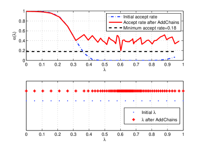
Figure 1: (Color online) Illustration of the AddChains algorithm on an $N=2048$ Ising spin system. In the bottom graph, we show the grid of initial linearly-spaced parameters and the resultant $\lambda$ after AddChains. The top graph plots the initial and final estimated swap rates after $70000$ sweeps of PT (in the left side of the plot, the blue and red lines are superimposed.) Around the region with $\lambda\in[0.5,0.8]$ the initial estimated swap rate plunged as low as $\approx e^{-79}$; after the parameter addition, all intervals had swaps taking place over the criterion rate, shown by the black dotted line. The initial grid consisted of $20$ parameters, to which 46 were added by the algorithm.

First we demonstrate how Algorithm 2 performed. AddChains was called on this system using a target swap threshold of $18\%$, $70000$ sweeps of PT, and $20$ chains to start. Figure 1 shows both how the acceptance rates responded to the interspersion and the particular locations in $\lambda$ space that parameters were added. The estimator of the swap rates at the initial parameter spacing produced $\widehat{L}$ as low as $-130$; thus in the $70000$ sweeps we performed, actually observing any swaps in such an interval is virtually impossible. The lower plot in Figure 1 shows where parameters were added to achieve the target; note the concentration around $\lambda\approx 0.6$. Our rough algorithm succeeded in achieving the target rate in all intervals.

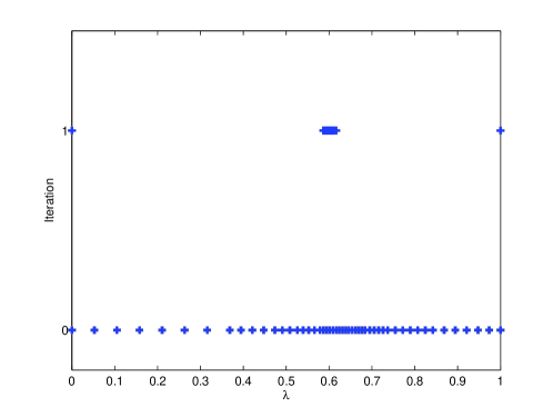
(a)

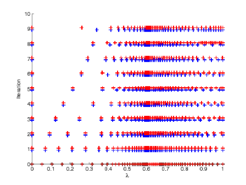
(b)

Figure 2: (Color online) Illustration of the progression of the parameters using the original FOPT algorithm and the one with our modifications on the $N=2048$ Ising spin system discussed in the text. Both algorithms began with the $\lambda$ spacings generated by AddChains; all replica were initialized with the ground state. At left, we see that in a single iteration, FOPT spaces all the parameters around $\lambda\approx 0.6$, resulting in very wide intervals between the endpoints. The algorithm could thus not proceed past this point because the replica in the middle could no longer visit either terminus; consequently $f$ was mathematically undefined. Our algorithm’s output appears at right. At each iteration step the resultant $\lambda$ using a smoothed version of $f$ in FOPT is shown in blue; the $\lambda$ returned when those parameters are passed to the PostProcess algorithm appear in red. Note that to keep the swap rate over the threshold of $3\%$, PostProcess often “pulled” parameters back if it predicted that the interval was too wide.

In Figure 2 a run of the initial FOPT algorithm and our stabilized version are shown. For our algorithm, we used the fairly strong smoothing value of $w=0.75$; the number of PT sweeps was constant at $200000$ in each iteration. For PostProcess, the minimum interval swap rate was set to $3\%$. The details can be read from the caption in the Figure, but the essential point is that the original algorithm aggressively spaces the parameters in such a way that the recursion cannot proceed past a single iteration. For all but the endpoint parameters, a PT run of realistic length using such $\{\lambda\}$ would give $n_{up}=n_{down}=0$. For illustration, in Figure 3 we show the progression of $f$ (not $f_{smooth}$ ) at different iterations of our method. Even on this highly troublesome instance, the parameters were finally spaced in such a way that enough round-trips took place to allow accurate estimation of the minimum excitation gap.

Figure 3: (Color online) Progress of the upward-moving fraction $f$ when our algorithm is applied to the $N=2048$ Ising spin system discussed in the text. Note the abrupt decline when PT is run with the results of AddChains. Subsequent iterations progressively make $f$ closer to the desired form, namely a straight line. $200000$ PT sweeps were used to gather the $f$ statistics at each iteration.

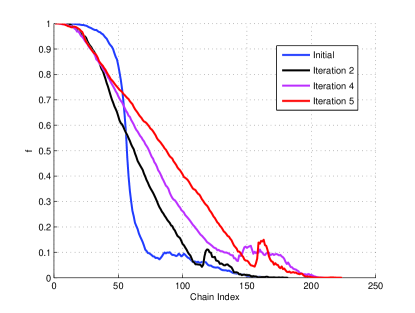
Figure 4: (Color online) Progress of the upward-moving fraction $f$ when the algorithm is applied to the $N=24576$ Ising spin system discussed in the text.

To demonstrate efficacy on the typical system sizes we were ultimately interested in simulating, in Figure 4 we present results of the evolution of $f$ on an $N=24576$ spin model resulting from representing a $96$ spin quantum system with 256 Trotter slices. The results were obtained using the same simulation parameter settings as those used for the previously-discussed 16-spin system. The resultant parameter spacing again allowed sufficiently good PT performance for us to obtain high-quality Monte Carlo data.

6 Conclusion

We have presented improvements to the problem of iterative parameter selection for PT. Our contribution has consisted of three parts: first, an initialization strategy to place parameters in a reasonable manner when no a priori information is known about the problem domain; second, the introduction of damping mechanisms to the FOPT algorithm of [3] that assist in tackling the problem of instability; third a post-processing procedure that prevents the algorithm from malfunctioning. We demonstrated the effectiveness of the method by showing experiments on a particularly difficult quantum spin system represented as a classical Ising model with $2048$ spins. We have tested our algorithm on much bigger systems with satisfactory results.

Acknowledgements

We would like to thank Helmut Katzgraber, Peter Young, Mohammad Amin, and Geordie Rose for valuable discussions and insights.

References

- [1] K. Hukushima and K. Nemoto. Exchange monte carlo method and application to spin glass simulations. Technical Report cond-mat/9512035, Dec 1995.
- [2] Y. Iba. Extended ensemble monte carlo. International Journal of Modern Physics C, 12:623, 2001.
- [3] H. G. Katzgraber, S. Trebst, D. A. Huse, and M. Troyer. Feedback-optimized parallel tempering monte carlo. Journal of Statistical Mechanics: Theory and Experiment, 2006(03):P03018, 2006.
- [4] W. Nadler and U. H. E. Hansmann. Generalized ensemble and tempering simulations: A unified view. Phys. Rev. E, 75(2):026109, Feb 2007.
- [5] C. Predescu, M. Predescu, and C. V. Ciobanu. The incomplete beta function law for parallel tempering sampling of classical canonical systems. The Journal of Chemical Physics, 120(9):4119–4128, 2004.
- [6] M. Suzuki. Relationship between d-dimensional quantal spin systems and (d+1)-dimensional ising system : Equivalence, critical exponents and systematic approximants of the partition function and spin correlations. Progress of theoretical physics, 56(5):1454–1469, 19761125.
- [7] S. Trebst, D. A. Huse, and M. Troyer. Optimizing the ensemble for equilibration in broad-histogram monte carlo simulations. Phys. Rev. E, 70(4):046701, Oct 2004.
- [8] A. P. Young, S. Knysh, and V. N. Smelyanskiy. Size dependence of the minimum excitation gap in the quantum adiabatic algorithm. Phys. Rev. Lett., 101(17):170503, Oct 2008.