Approximation Algorithms for the Capacitated Domination Problem

Abstract

We consider the Capacitated Domination problem, which models a service-requirement assignment scenario and is also a generalization of the well-known Dominating Set problem. In this problem, given a graph with three parameters defined on each vertex, namely cost, capacity, and demand, we want to find an assignment of demands to vertices of least cost such that the demand of each vertex is satisfied subject to the capacity constraint of each vertex providing the service.

In terms of polynomial time approximations, we present logarithmic approximation algorithms with respect to different demand assignment models for this problem on general graphs, which also establishes the corresponding approximation results to the well-known approximations of the traditional Dominating Set problem. Together with our previous work, this closes the problem of generally approximating the optimal solution. On the other hand, from the perspective of parameterization, we prove that this problem is W[1]-hard when parameterized by a structure of the graph called treewidth. Based on this hardness result, we present exact fixed-parameter tractable algorithms when parameterized by treewidth and maximum capacity of the vertices. This algorithm is further extended to obtain pseudo-polynomial time approximation schemes for planar graphs.

1 Introduction

For decades, Dominating Set problem has been one of the most fundamental and well-known problems in both graph theory and combinatorial optimization. Given a graph $G=(V,E)$ and an integer $k$, Dominating Set asks for a subset $D\subseteq V$ whose cardinality does not exceed $k$ such that every vertex in the graph either belongs to this set or has a neighbor which does. As this problem is known to be NP-hard, approximation algorithms have been proposed in the literature. On one hand, a simple greedy algorithm is shown to achieve a guaranteed ratio of $O(\ln n)$ [5, 17, 21], where $n$ is the number of vertices, which is later proven to be the approximation threshold by Feige [9]. On the other hand, algorithms based on dual-fitting provide a guaranteed ratio of $\Delta$ [15], where $\Delta$ is the maximum degree of the vertices of the graph.

In addition to polynomial time approximations, Dominating Set has its special place from the perspective of parameterized complexity as well [8, 10, 22]. In contrast to Vertex Cover, which is fixed-parameter tractable (FPT), Dominating Set has been proven to be W[2]-complete when parameterized by solution size, in the sense that no fixed-parameter algorithm exists (with respect to solution size) unless FPT=W[2]. Though Dominating Set is a fundamentally hard problem in the parameterized $W$-hierarchy, it has been used as a benchmark problem for developing sub-exponential time parameterized algorithms [1, 6, 11] and linear size kernels have been obtained in planar graphs [2, 10, 12, 22], and more generally, in graphs that exclude a fixed graph $H$ as a minor.

Besides Dominating Set problem itself, a vast body of work has been proposed in the literature, considering possible variations from purely theoretical aspects to practical applications. See [14, 23] for a detailed survey. In particular, variations of Dominating Set problem occur in numerous practical settings, ranging from strategic decisions, such as locating radar stations or emergency services, to computational biology and to voting systems. For example, Haynes et al. [13] considered Power Domination Problem in electric networks [13, 20] while Wan et al. [24] considered Connected Domination Problem in wireless ad hoc networks.

Motivated by a general service-requirement assignment model, Kao et al., [18] considered a generalized domination problem called Capacitated Domination. In this problem, the input graph is given with tri-weighted vertices, referred to as cost, capacity, and demand, respectively. The demand of a vertex stands for the amount of service it requires from its adjacent vertices (including itself) while the capacity of a vertex represents the amount of service it can provide when it’s selected as a server. The goal of this problem is to find a dominating multi-set as well as a demand assignment function such that the overall cost of the multi-set is minimized. For different underlying applications, there are two different demand assignment models, namely splittable demand model and unsplittable demand model, depending on whether or not the demand of a vertex is allowed to be served by different vertices. Moreover, there has been work studying the variation when the number of copies, or multiplicity of each vertex in the dominating multi-set, is limited, referred to as hard capacity, and as soft capacity when no such limit is specified. Kao et al., [18] considered the soft capacitated domination problem with splittable demand and provided a $(\Delta+1)$-approximation for general graphs, where $\Delta$ is the degree of the graph. For special graph classes, they proved that even when the input graph is restricted to a tree, the soft capacitated domination problem with splittable demand remains NP-hard, for which they also presented a polynomial time approximation scheme. Dom et al., [7] considered the hard capacitated domination problem with uniform demand and showed that this problem is W[1]-hard even when parameterized by treewidth and solution size.

In this paper, we consider the (soft) Capacitated Domination problem and present logarithmic approximation algorithms with respect to different demand assignment models on general graphs. Specifically, we provide a $(\ln n)$-approximation for weighted unsplittable demand model, a $(4\ln n+2)$-approximation for weighted splittable demand model, and a $(2\ln n+1)$-approximation for unweighted splittable demand model, where $n$ is the number of vertices. Together with the $(\Delta+1)$-approximation result given by Kao et al., [18], this establishes a corresponding near-optimal approximation result to the original Dominating Set problem. Although the result may look natural, the greedy choice we make is not obvious when non-uniform capacity as well as non-uniform demand is taken into consideration. On the other hand, from the perspective of parameterization, we prove that this problem is W[1]-hard when parameterized by a structure of the graph, called the treewidth, and present exact FPT algorithms when parameterized by the treewidth and the maximum capacity of the vertices. This algorithm is further extended to obtain pseudo-polynomial time approximation schemes for planar graphs, based on a framework due to Baker [3].

The rest of this paper is organized as follows. In Section 2, we give formal definitions and notation adopted in the paper. In Section 3, we present our ideas and algorithms that achieve the aforementioned approximation guarantees. We present the parameterized results in Section 4 and conclude by listing some future work in Section 5.

2 Preliminary

We assume that all the graphs considered in this paper are simple and undirected. Let $G=(V,E)$ be a graph with vertex set $V$ and edge set $E$. A vertex $v\in V$ is said to be adjacent to a vertex $u\in V$ if $(u,v)\in E$. The set of neighbors of a vertex $v\in V$ is denoted by $N_{G}(v)=\{u:(u,v)\in E\}$. The closed neighborhood of $v\in V$ is denoted by $N_{G}[v]=N_{G}(v)\cup\{v\}$. The subscript $G$ in $N_{G}[v]$ will be omitted when there is no confusion.

Consider a graph $G=(V,E)$ with tri-weighted vertices, referred to as the cost, the capacity, and the demand of each vertex $u\in V$, denoted by $w(u)$, $c(u)$, and $d(u)$, respectively. Let $D$ denote a multi-set of vertices of $V$ and for any vertex $u\in V$, let $x_{D}(u)$ denote the multiplicity of $u$ or the number of times of $u$ in $D$. The cost of $D$, denoted $w(D)$, is defined to be $w(D)=\sum_{u\in D}w(u)\cdot x_{D}(u)$.

Definition 1 (Capacitated Dominating Set).

A vertex multi-subset $D$ is said to be a feasible capacitated dominating set with respect to a demand assignment function $f$ if the following conditions hold.

• Demand constraint: $\sum_{u\in N_{G}[v]}f(v,u)\geq d(v)$, for each $v\in V$.

• Capacity constraint: $\sum_{u\in N_{G}[v]}f(u,v)\leq c(v)\cdot x_{D}(v)$, for each $v\in V$.

Given a problem instance, the capacitated domination problem asks for a capacitated dominating multi-set $D$ and demand assignment function $f$ such that $w(D)$ is minimized. For unsplittable demand model we require that $f(u,v)$ is either $0$ or $d(u)$ for each edge $(u,v)\in E$. Note that since it is already NP-hard to compute a feasible demand assignment function from a given feasible capacitated dominating multi-set when the demand cannot be split, it is natural to require the demand assignment function be specified, in addition to the optimal vertex multi-set itself.

Parameterized complexity is a well-developed framework for studying the computationally hard problem [8, 10, 22]. A problem is called fixed-parameter tractable (FPT) with respect to a parameter $k$ if it can be solved in time $f(k)\cdot n^{O(1)}$, where $f$ is a computable function depending only on $k$. Problems (along with its defining parameters) belonging to W[t]-hard for any $t\geq 1$ are believed not to admit any FPT algorithms (with respect to the specified parameters). Now we define the notion of parameterized reduction.

Definition 2.

Let $A$ and $B$ be two parameterized problems. We say that $A$ reduces to $B$ by a standard parameterized reduction if there exists an algorithm $\Phi$ that transforms $(x,k)$ into $(x^{\prime},g(k))$ in time $f(k)\cdot\left|x\right|^{\alpha}$, where $f,g:\mathcal{N}\rightarrow\mathcal{N}$ are arbitrary functions and $\alpha$ is a constant independent of $\left|x\right|$ and $k$, such that $(x,k)\in A$ if and only if $(x^{\prime},g(k))\in B$.

Next we define the concept of tree decomposition [4, 19].

Definition 3 (Tree Decomposition of a Graph).

A tree decomposition of a graph $G=(V,E)$ is a pair $(X=\left\{X_{i}:i\in I\right\},T=(I,F))$ where each node $i\in I$ has associated with it a subset of vertices $X_{i}\subseteq V$, called the bag of $i$, such that

1. Each vertex belongs to at least one bag: $\bigcup_{i\in I}X_{i}=V$.

2. For all edges, there is a bag containing both its end-points.

3. For all vertices $v\in V$, the set of nodes $\{i\in I:v\in X_{i}\}$ induces a subtree of $T$.

The width of a tree decomposition is $\max_{i\in I}\left|X_{i}\right|$. The treewidth of a graph $G$ is the minimum width over all tree decompositions of $G$.

Definition 4 (Nice Tree Decomposition [19]).

A tree decomposition $(X,T)$ is a nice tree decomposition if one can root $T$ in such a way that each node $i\in I$ is of one of the four following types.

1. Leaf: node $i$ is a leaf of $T$, and $\left|X_{i}\right|=1$.

2. Join: node $i$ has exactly two children, say $j_{1}$ and $j_{2}$, and $X_{i}=X_{j_{1}}=X_{j_{2}}$.

3. Introduce: node $i$ has exactly one child, say $j$, and there is a vertex $v\in V$ such that $X_{i}=X_{j}\cup\left\{v\right\}$.

4. Forget: node $i$ has exactly one child, say $j$, and there is a vertex $v\in V$ such that $X_{j}=X_{i}\cup\left\{v\right\}$.

Given a tree decomposition of width $k$, a nice tree decomposition of the same width can be found in linear time [19].

3 Logarithmic Approximation

In this section, we present logarithmic approximation algorithms for capacitated domination problems with respect to different cost and demand models. Specifically, we provide a $(\ln n)$-approximation for weighted unsplittable demand model, a $(4\ln n+2)$-approximation for weighted splittable demand model, and a $(2\ln n+1)$-approximation for unweighted splittable demand model, where $n$ is the number of vertices.

The main idea is based on greedy approach in the sense that we keep choosing a vertex with the best efficiency in each iteration until the whole graph is dominated. By best efficiency we mean the maximum cost-efficiency ratio defined for each vertex in the remaining graph. We describe the results in more detail in the following subsections.

3.1 Weighted Unsplittable Demand

In this section, we consider the weighted capacitated domination problem with unsplittable demand and provide a simple greedy algorithm that achieves the approximation guarantee of $\ln n$.

Let $U$ be the set of vertices which are not dominated yet. Initially, we have $U=V$. For each vertex $u\in V$, let $N_{ud}[u]=U\cap N[u]$ be the set of undominated vertices in the closed neighborhood of $u$. Without loss of generality, we shall assume that the elements of $N_{ud}[u]$, denoted by $v_{u,1},v_{u,2},\ldots,v_{u,{|N_{ud}[u]|}}$, are sorted in non-decreasing order of their demands in the remaining section.

In each iteration, the algorithm chooses a vertex of the most efficiency from $V$, where the efficiency of a vertex, say $u$, is defined by the largest effective-cost ratio of the number of vertices dominated by $u$ over the total cost. That is,

$$\max_{1\leq i\leq|N_{ud}[u]|}\frac{i}{w(u)\cdot x_{u}(i)},$$

where

$$x_{u}(i)=\left\lceil\frac{\sum_{1\leq j\leq i}d(v_{u,j})}{c(u)}\right\rceil$$

is the number of copies of $u$ selected in order to dominate $v_{u,1},v_{u,2},\ldots,$ and $v_{u,i}$. A high-level description of this algorithm is presented in Figure 1.

  Algorithm Unsplit-Log-Approx

1:  $U\longleftarrow V$

2:  while $U\neq\phi$ do

3:     Pick a vertex in $V$ with the most efficiency, say $u$.

4:     let $k=\arg\max_{1\leq i\leq|N_{ud}[u]|}\frac{i}{w(u)\cdot x_{u}(i)}$.

5:     Assign the demand of each vertex in $\{v_{u,1},v_{u,2},\ldots,v_{u,k}\}$ to $u$ and remove them from $U$.

6:  end while

7:  compute from the assignment the weight of the dominating set, and return the result.

 

Figure 1: The pseudo-code for the weighted unsplittable demand model.

In iteration $j$, let $OPT_{j}$ be the cost of the optimal solution for the remaining problem instance, which is clearly upper bounded by the cost, $OPT$, of the optimal solution for the input instance. Let the number of undominated vertices at the beginning of iteration $j$ be $n_{j}$, and the number of vertices that are newly dominated in iteration $j$ be $k_{j}$.

Denote by $S_{j}$ the cost in iteration $j$. Note that $S_{j}=w(u)\cdot x_{u}(k_{j})$, where $u$ is the most efficient vertex chosen in iteration $j$. Assume that the algorithm repeats for $m$ iterations. We have the following lemma.

Lemma 1.

For each $j$, $1\leq j\leq m$, we have $S_{j}\leq\frac{k_{j}}{n_{j}}\cdot OPT_{j}$.

Proof.

Since we always choose the vertex with the maximum efficiency, the efficiency is no less than that of each vertex chosen in $OPT_{j}$, which is no less than the average of $OPT_{j}$. Therefore we have $\frac{k_{j}}{S_{j}}\geq\frac{n_{j}}{OPT_{j}}$ and the lemma follows. ∎

Theorem 2.

Algorithm Unsplit-Log-Approx computes a $(\ln n)$-approximation for weighted capacitated domination problem with unsplittable demands in $O(n^{3})$ time, where $n$ is the number of vertices.

Proof.

To see that the algorithm produces a logarithmic approximation, take the sum over each $S_{j}$, $1\leq j\leq m$ and observe that $n_{j+1}=n_{j}-k_{j}$, we have

$$\sum_{1\leq j\leq m}S_{j}\leq\sum_{1\leq j\leq m}\frac{k_{j}}{n_{j}}\cdot OPT_{j}\leq\left(\sum_{1\leq j\leq n}\frac{1}{j}\right)\cdot OPT\leq\ln n\cdot OPT.$$

To see the time complexity, notice that it requires $O(n)$ time to compute a most efficient move for each vertex, which leads to an $O(n^{2})$ computation for the most efficient choice in each iteration. The number of iterations is upper bounded by $O(n)$ since at least one vertex is satisfied in each iteration. ∎

3.2 Weighted Splittable Demand

In this section, we present an algorithm that produces a $(4\ln n+2)$-approximation for the weighted capacitated domination problem with splittable demand. The difference between this algorithm and the previous one lies in the way we handle the demand assignment. In each iteration the demand of a vertex may be partially served. The unsatisfied portion of the demand is called residue demand. For each vertex $u\in V$, let $rd(u)$ be the residue demand of $u$. $rd(u)$ is set equal to $d(u)$ initially, and will be updated accordingly when a portion of the residue demand is assigned. $u$ is said to be completely satisfied when $rd(u)=0$.

We will inherit the notation used in the previous section. We assume that the elements of $N_{ud}[u]$, written as $v_{u,1},v_{u,2},\ldots,v_{u,|N_{ud}[u]|}$, are sorted according to their demands in non-decreasing order.

In each iteration, the algorithm performs two greedy choices. First, the algorithm chooses the vertex of the most efficiency from $V$, where the efficiency is defined similarly as in the previous section with some modification since the demand is splittable.

  Algorithm Split-Log-Approx

1:  $rd(u)\longleftarrow d(u)$, and $map(u)\longleftarrow\phi$ for each $u\in V$.

2:  while there exist vertices with non-zero residue demand do

3:     // $1^{st}$ greedy choice

4:     Pick a vertex in $V$ with the most efficiency, say $u$.

5:     if $j_{u}$ equals $0$ then

6:        Assign this amount $c(u)\cdot\left\lfloor\frac{rd(v_{u,1})}{c(u)}\right\rfloor$ of residue demand of $v_{u,1}$ to $u$.

7:        $map(v_{u,1})\longleftarrow\left\{u\right\}$

8:     else

9:        Assign the residue demands of the vertices in $\{v_{u,1},v_{u,2},\ldots,v_{u,j_{u}}\}$ to $u$.

10:        if $j_{u}<\left|N_{ud}[u]\right|$ then

11:           Assign this amount $c(u)-\sum_{i=1}^{j_{u}}rd(v_{u,i})$ of residue demand of $v_{u,j_{u}+1}$ to $u$.

12:           $map(v_{u,j_{u}+1})\longleftarrow map(v_{u,j_{u}+1})\cup\left\{u\right\}$

13:        end if

14:     end if

15:     

16:     // $2^{nd}$ greedy choice

17:     if there is a vertex $u$ with $0<rd(u)<\frac{1}{2}\cdot d(u)$ then

18:        Satisfy $u$ by doubling the demand assignment of $u$ to vertices in $map(u)$.

19:     end if

20:  end while

21:  compute from the assignment the cost of the dominating set, and return the result.

 

Figure 2: The pseudo-code for the weighted splittable demand model.

For each vertex $u\in V$, let $j_{u}$ with $0\leq j_{u}\leq\left|N_{ud}[u]\right|$ be the maximum index such that $c(u)\geq\sum_{i=1}^{j_{u}}rd(v_{u,i})$. Let $X(u)=\sum_{i=1}^{j_{u}}\frac{rd(v_{u,i})}{d(v_{u,i})}$ be the sum of the effectiveness over the vertices whose residue demand could be completely served by a single copy of $u$. In addition, we let

$$Y(u)=\frac{c(u)-\sum_{i=1}^{j_{u}}rd(v_{u,i})}{d(v_{u,j_{u}+1})}$$

if $j_{u}<\left|N_{ud}[u]\right|$ and $Y(u)=0$ otherwise. The efficiency of $u$ is defined as $\frac{X(u)+Y(u)}{w(u)}$.

Second, the algorithm maintains for each vertex $u\in V$ a set of vertices, denoted by $map(u)$, which consists of vertices that have partially served the demand of $u$ before $u$ is completely satisfied. That is, for each $v\in map(u)$ we have a non-zero demand assignment of $u$ to $v$. Whenever there exists a vertex $u$ whose residue demand is below half of its original demand, i.e., $0<rd(u)<\frac{1}{2}\cdot d(u)$, after the first greedy choice, the algorithm immediately doubles the demand assignment of $u$ to the vertices in $map(u)$. Note that in this way, we can completely satisfy the demand of $u$ since $\sum_{v\in map(u)}f(u,v)>\frac{1}{2}\cdot d(u)$ . A high-level description of this algorithm is presented in Figure 2.

Observation 1.

After each iteration, the residue demand of each unsatisfied vertex is at least half of its original demand.

Clearly, the observation holds in the beginning when the demand of each vertex is not yet assigned. For later stages, we argue that the algorithm properly maintains $map$ so that in our second greedy choice, whenever there exists a vertex $u$ for which $0<rd(u)<\frac{1}{2}\cdot d(u)$, it’s always sufficient to double the demand assignment $f(u,v)$ of $u$ to $v$ for each $v\in map(u)$. If $map(u)$ is only modified under the condition $0<j_{v}<\left|N_{ud}[v]\right|$, (line 12 in Figure 2), then $map(u)$ contains exactly the set of vertices that have partially served $u$. As mentioned above, since $rd(u)<\frac{1}{2}\cdot d(u)$, it’s sufficient to double the demand assignment in this case so $d(u)$ is completely satisfied. If $map(u)$ is reassigned through the condition $j_{v}=0$ for some stage, then we have $c(v)<rd(u)\leq d(u)$. Since we assign this amount $c(v)\cdot\left\lfloor rd(u)/c(v)\right\rfloor$ of residue demand of $u$ to $v$, this leaves at most half of the original residue demand and $u$ will be satisfied by doubling this assignment.

By the description given above, we conclude that the algorithm produces a feasible demand assignment as well as a feasible capacitated dominating set. Let the cost incurred by the first greedy choice be $S_{1}$ and the cost by the second choice be $S_{2}$. To see that the solution achieves the desired approximation guarantee, first notice that $S_{2}$ is bounded above by $S_{1}$, for what we do in the second choice is merely to satisfy the residue demand of a vertex, if there exists one, by doubling its previous demand assignment.

In the following, we will bound the cost $S_{1}$. For each iteration $j$, let $u_{j}$ be the vertex of the maximum efficiency and $OPT_{j}$ be the cost of the optimal solution for the remaining problem instance. Let $n_{j}=\sum_{u\in V}rd(u)/d(u)$ denote the sum of effectiveness of each vertex in the remaining problem instance at the beginning of this iteration. Let $S_{1,j}$ be the cost incurred by the first greedy choice in iteration $j$. Assume that the algorithm repeats for $m$ iterations. We have the following lemma.

Lemma 3.

For each $j$, $1\leq j\leq m$, we have $S_{1,j}\leq\frac{n_{j}-n_{j+1}}{n_{j}}\cdot OPT_{j}$, where $n_{j}-n_{j+1}$ is the effectiveness covered by $u_{j}$ in iteration $j$.

Proof.

The optimality of our choice in each iteration is obvious since we assume that the elements of $N_{ud}[u]$ are sorted according to their original demands. Note that only in the case $c(u)<rd(v_{u,1})$, the algorithm could possibly take more than one copy. In this case the efficiency of our choice remains unchanged since the cost and the effectiveness covered by $u$ grows by the same factor. Therefore the efficiency of our choice, $(n_{j}-n_{j+1})/S_{1,j}$, is always no less than that of the optimal solution, which is $n_{j}/OPT_{j}$, and the lemma follows. ∎

Observation 2.

We have $n_{j}-n_{j+1}\geq\frac{1}{2}$ for each $1\leq j\leq m$.

Proof.

For iteration $j$, $1\leq j\leq m$, let $u$ be the vertex of the maximum efficiency. Observe that $v_{u,1}$ will be satisfied after this iteration. By Observation 1, we have $rd(v_{u,1})/d(v_{u,1})>\frac{1}{2}$. The lemma follows. ∎

By Lemma 3 we have

$$\sum_{j=1}^{m}S_{1,j}\leq\sum_{j=1}^{m-1}\frac{n_{j}-n_{j+1}}{n_{j}}\cdot OPT_{j}+\frac{n_{m}}{n_{m}}\cdot OPT_{m}\leq\left(\sum_{j=1}^{m-1}\frac{\left\lceil n_{j}-n_{j+1}\right\rceil}{\left\lfloor n_{j}\right\rfloor}+1\right)\cdot OPT,$$

since $\left\lfloor r\right\rfloor\leq r\leq\left\lceil r\right\rceil$ for any real number $r$ and $OPT_{j}\leq OPT$ for each $1\leq j\leq m$.

Lemma 4.

$\sum_{j=1}^{m-1}\left\lceil n_{j}-n_{j+1}\right\rceil/\left\lfloor n_{j}\right\rfloor\leq 2\ln n$

Proof.

Note that by Observation 1 and Observation 2, we have $n_{j}>1$ for all $j<m$. We will argue that this series together constitutes at most two harmonic series. By expanding the summand we have

$$\frac{\left\lceil n_{j}-n_{j+1}\right\rceil}{\left\lfloor n_{j}\right\rfloor}\leq\frac{1}{\left\lfloor n_{j}\right\rfloor}+\frac{1}{\left\lfloor n_{j}\right\rfloor-1}+\ldots+\frac{1}{\left\lfloor n_{j}\right\rfloor-\lceil n_{j}-n_{j+1}\rceil+1}.$$

Since $\lfloor n_{j+1}\rfloor=\lfloor n_{j}-(n_{j}-n_{j+1})\rfloor\leq\lfloor n_{j}\rfloor-\lfloor n_{j}-n_{j+1}\rfloor\leq\lfloor n_{j}\rfloor-\lceil n_{j}-n_{j+1}\rceil+1$, the repetitions only occur at the first term and the last term if we expand the summation. By Observation 2, the decrease of $n_{j}$ to $n_{j+1}$ is at least half. Therefore, the term $\left\lfloor n_{j}\right\rfloor-\left\lceil n_{j}-n_{j+1}\right\rceil+1$ will never occur more than twice in the expansion. We conclude that $\sum_{j=1}^{m-1}\left\lceil n_{j}-n_{j+1}\right\rceil/\left\lfloor n_{j}\right\rfloor\leq 2\ln n$ ∎

Theorem 5.

Algorithm Split-Log-Approx computes a $(4\ln n+2)$-approximation in $O(n^{3})$ time, where $n$ is the number of vertices, for weighted capacitated domination problem with splittable demands.

3.3 Unweighted Splittable Demand

In this section, we consider the unweighted capacitated domination problem with splittable demand and present a $(2\ln n+1)$-approximation. In this case the weight $w(v)$ of each vertex $v\in V$ is considered to be 1 and the cost of the capacitated domination multiset $D$ corresponds to the total multiplicity of the vertices in $D$. To this end, we first make a greedy reduction on the problem instance by spending at most $1\cdot OPT$ cost such that it takes at most one copy to satisfy each remaining unsatisfied vertex. Then we show that a $(2\ln n)$-approximation can be computed for the remaining problem instance, based on the same framework of Section 3.2.

For each $u\in V$, let $g_{u}$ be the vertex in $N[u]$ with the maximum capacity. First, for each $u\in V$, we assign this amount $c(g_{u})\cdot\left\lfloor\frac{d(u)}{c(g_{u})}\right\rfloor$ of the demand of $u$ to $g_{u}$. Let the cost of this assignment be $S$, then we have the following lemma.

Lemma 6.

We have $S\leq OPT$, where $OPT$ is the cost of the optimal solution.

Proof.

Notice that an optimal solution $O^{*}$ for the relaxation of this problem, where fractional copies are allowed, can be obtained by assigning the demand $d(u)$ of $u$ to $g_{u}$. Since $S\leq O^{*}$ and $O^{*}\leq OPT$, the lemma follows. ∎

In the following, we will assume that $d(u)\leq c(g_{u})$, for each $u\in V$. The algorithm of Section 3.2 is slightly modified. In particular, for the second greedy choice, whenever $rd(u)<d(u)$ for some vertex $u\in V$, we immediately assign the residue demand of $u$ to $g_{u}$. A high-level description of this algorithm is presented in Figure 3.

  Algorithm Unweighted-Split-Log-Approx

1:  For each $u\in V$, assign $c(g_{u})\cdot\left\lfloor\frac{d(u)}{c(g_{u})}\right\rfloor$ demands of $u$ to $g_{u}$, where $g_{u}\in N[u]$ has the maximum capacity.

2:  Reset the demands of the instance by setting $d(u)\longleftarrow rd(u)$ for each $u\in V$.

3:  while there exist vertices with non-zero residue demand do

4:     // $1^{st}$ greedy choice

5:     Pick a vertex in $V$ with the most efficiency, say $u$.

6:     Assign the demands of the vertices in $\{v_{u,1},v_{u,2},\ldots,v_{u,j_{u}}\}$ to $u$.

7:     if $j_{u}<\left|N_{ud}[u]\right|$ then

8:        Assign this amount $c(u)-\sum_{i=1}^{j_{u}}rd(v_{u,i})$ of the residue demand of $v_{u,j_{u}+1}$ to $u$.

9:     end if

10:     

11:     // $2^{nd}$ greedy choice

12:     if there is a vertex $u$ with $0<rd(u)<d(u)$ then

13:        Satisfy $u$ by assigning the residue demand of u to $g_{u}$.

14:     end if

15:  end while

16:  compute from the assignment the cost of the dominating set, and return the result.

 

Figure 3: The pseudo-code for the unweighted splittable demand model.

Observation 3.

We have $n_{j}-n_{j+1}\geq 1$ for each $1\leq j\leq m$.

Proof.

Observe that in each iteration, at least one vertex is satisfied and the residue demand of each unsatisfied vertex is equal to its original demand. ∎

Clearly, $S_{2}$ is bounded above by $S_{1}$, as we always take one copy for the first greedy choice and at most one copy for the second greedy choice in each iteration. By Observation 3 and the fact that $n_{j}$ is integral for each $1\leq j\leq m$, we have

$$\sum_{j=1}^{m}S_{2,j}\leq\sum_{j=1}^{m}\frac{n_{j}-n_{j+1}}{n_{j}}\cdot OPT_{j}\leq\ln n\cdot OPT,$$

and $S+\sum_{j=1}^{m}\left(S_{1,j}+S_{2,j}\right)\leq(2\ln n+1)\cdot OPT.$

We conclude the result as the following theorem.

Theorem 7.

Algorithm Unweight-Split-Log-Approx computes a $(2\ln n+1)$-approximation in $O(n^{3})$ time for weighted capacitated domination problem with unsplittable demands, where $n$ is the number of vertices.

4 Parameterized Results

4.1 Hardness Results

In this section we show that Capacitated Domination Problem is W[1]-hard when parameterized by treewidth by making a reduction from k-Multicolor Clique, a restriction of k-Clique problem.

Definition 5 (Multicolor Clique).

Given an integer $k$ and a connected undirected graph $G=\left(\bigcup_{i=1}^{k}V[i],E\right)$ such that $V[i]$ induces an independent set for each $i$, the Multicolor Clique problem asks whether or not there exists a clique of size $k$ in $G$.

Given an instance $(G,k)$ of Multicolor Clique, we will show how an instance $\mathcal{G}=(\mathcal{V},\mathcal{E})$ of Capacitated Domination with treewidth $O(k^{2})$ can be built such that $G$ has a clique of size $k$ if and only if $\mathcal{G}$ has a capacitated dominating set of cost at most $k^{\prime}=(3k^{2}-k)/2$. For convenience, we shall distinguish the vertices of $\mathcal{G}$ by referring to them as nodes.

Let $N$ be the number of vertices. Without loss of generality, we label the vertices of $G$ by numbers, denoted $label(v)$, $v\in V$, between $1$ and $N$. For each $i\neq j$, let $E[i,j]$ denote the set of edges between $V[i]$ and $V[j]$. The graph $\mathcal{G}$ is defined as follows. For each $i$, $1\leq i\leq k$, we create a node $x_{i}$ with $w(x_{i})=k^{\prime}+1$, $c(x_{i})=0$, and $d(x_{i})=1$. For each $u\in V[i]$, we have a node $\overline{u}$ with $w(\overline{u})=1$, $c(\overline{u})=1+(k-1)N$, and $d(\overline{u})=0$. We also connect $\overline{u}$ to $x_{i}$. For convenience, we refer to the star rooted at $x_{i}$ as vertex star $T_{i}$.

Similarly, for each $1\leq i<j\leq k$, we create a node $y_{ij}$ with $w(y_{ij})=k^{\prime}+1$, $c(x_{i})=0$, and $d(x_{i})=1$. For each $e\in E[i,j]$ we have a node $\overline{e}$ with $w(\overline{e})=1$, $c(\overline{e})=1+2N$, and $d(\overline{e})=0$. We connect $\overline{e}$ to $y_{ij}$. We refer to the star rooted at $y_{ij}$ as edge star $T_{ij}$. The selection of nodes in $T_{i}$ and $T_{ij}$ in the capacitated dominating set will correspond to the choices made in selecting the vertices that form a clique in $G$.

In addition, for each $i\neq j$, $1\leq i,j\leq k$, we create two bridge nodes $b^{1}_{i,j}$, $b^{2}_{i,j}$ with $w(b^{1}_{i,j})=w(b^{2}_{i,j})=1$ and $d(b^{1}_{i,j})=d(b^{2}_{i,j})=1$. The capacities of the bridge nodes are to be defined later. Now we describe the way how stars $T_{i}$ and $T_{ij}$ are connected to bridge nodes such that the reduction claimed above holds. For each $i\neq j$, $1\leq i,j\leq k$ and for each $v\in V[i]$, we create two propagation nodes $p^{1}_{v,i,j}$, $p^{2}_{v,i,j}$ and connect them to $\overline{v}$. Besides, we connect $p^{1}_{v,i,j}$ to $b^{1}_{i,j}$ and $p^{2}_{v,i,j}$ to $b^{2}_{i,j}$. We set $w(p^{1}_{v,i,j})=w(p^{2}_{v,i,j})=k^{\prime}+1$ and $c(p^{1}_{v,i,j})=c(p^{2}_{v,i,j})=0$. The demands of $p^{1}_{v,i,j}$ and $p^{2}_{v,i,j}$ are set to be $d(p^{1}_{v,i,j})=label(v)$ and $d(p^{2}_{v,i,j})=N-label(v)$. For each $1\leq i<j\leq k$ and for each $e=(u,v)\in E[i,j]$, we create four propagation nodes $p^{1}_{e,i,j}$, $p^{2}_{e,i,j}$, $p^{1}_{e,j,i}$, and $p^{2}_{e,j,i}$ with zero capacity and $k^{\prime}+1$ cost. Without loss of generality, we assume that $u\in V[i]$ and $v\in V[j]$. The demands of the four nodes are set as the following: $d(p^{1}_{e,i,j})=N-label(u)$, $d(p^{2}_{e,i,j})=label(u)$, $d(p^{1}_{e,j,i})=N-label(v)$, and $d(p^{2}_{e,j,i})=label(v)$. Finally, for each bridge node $b$, we set $c(b)=\sum_{u\in N[b]}d(b)-N$.

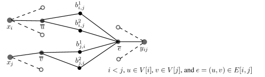
Figure 4: The connections between stars and bridge nodes.

Lemma 8.

The treewidth of $\mathcal{G}$ is $O(k^{2})$. Furthermore, $G$ admits a clique of size $k$ if and only if $\mathcal{G}$ admits a capacitated dominating set of cost at most $k^{\prime}=(3k^{2}-k)/2$.

Proof of Lemma 8..

Consider the set of bridge nodes, $Bridge=\bigcup_{i\neq j}\left\{b^{1}_{i,j}\cup b^{2}_{i,j}\right\}$. Since $\mathcal{G}\backslash Bridge$ is a forest and the removal of a vertex from a graph decreases the treewidth of the graph by at most one, the treewidth of $\mathcal{G}$ is upper bounded by the number of bridge nodes plus some constant, which is $O(k^{2})$.

Let $C$ be a clique of size $k$ in $G$. By choosing the bridge nodes, $b^{1}_{i,j}$ and $b^{2}_{i,j}$ for each $i\neq j$, $\overline{u}$ for each $u\in C$, and $\overline{e}$ for each $e\in C$ exactly once, we have a vertex subset of cost exactly $(3k^{2}-k)/2$. One can easily verify that this is also a feasible capacitated dominating multi-set for $\mathcal{G}$.

On the other hand, let $D$ be a capacitated donimating multi-set of cost at most $k^{\prime}$ in $\mathcal{G}$. First observe that none of the propagation nodes are chosen in $D$, otherwise the cost would exceed $k^{\prime}$. This implies $b^{1}_{i,j}\in D$ and $b^{2}_{i,j}\in D$ for each $i\neq j$. Note that this already contributes cost at least $k(k-1)$ to $D$ and the rest of the nodes in $D$ together contributes at most $k(k+1)/2$.

Similarly, we have $x_{i}\notin D$ and $y_{ij}\notin D$ for each $i\neq j$. Therefore, for each $1\leq i\leq k$, $\exists u\in V[i]$ such that $\overline{u}\in D$, and for each $i\neq j$, $\exists e\in E[i,j]$ such that $\overline{e}\in D$. Since we have $k(k-1)/2+k=k(k+1)/2$ such stars, exactly one node from each star is chosen to be included in $D$ and each node of $D$ is chosen exactly once. Next we argue that the nodes chosen in each star will correspond to a clique of size $k$ in $G$.

For each $1\leq i<j\leq k$, let $\overline{u}\in T_{i}$ and $\overline{v}\in T_{j}$ be the nodes chosen in $D$. Let $\overline{e}\in T_{ij}$ be the node chosen in $D$. In the following we shall prove that $e=(u,v)$. Since the capacity of $\overline{u}$ equals the sum of the demands over $N[\overline{u}]$, the closed neighborhood of $\overline{u}$, without loss of generality we can assume that the demands of nodes in $N[\overline{u}]$ are served by $\overline{u}$. Consider the bridge vertex $b^{1}_{ij}$ and the set $S=N[b^{1}_{ij}]\backslash N[\overline{u}]$. The demands of vertices in $S$ can only be served by either $b^{1}_{ij}$ or $\overline{e}$, as they are the only two vertices in $N[S]$ chosen to be included in $D$. In particular, vertices in $S$ apart from $p^{1}_{e,i,j}$ can only be served by $b^{1}_{ij}$. Notice that the sum of the demands in $S$ is $N-label(u)$ above the capacity of $b^{1}_{ij}$. Therefore we have $d(p^{1}_{e,i,j})\geq N-label(u)$, which implies $d(p^{2}_{e,i,j})\leq label(u)$ as well since we have $d(p^{1}_{e,i,j})+d(p^{2}_{e,i,j})=N$ by our setting.

By a symmetric argument on $b^{2}_{i,j}$ we obtain $d(p^{2}_{e,i,j})\geq label(u)$. Hence $d(p^{2}_{e,i,j})=label(u)$. By another symmetric argument on $b^{1}_{ji}$ and $b^{2}_{ji}$, we have $d(p^{2}_{e,j,i})=label(v)$. Therefore $e=(u,v)$ by our construction. ∎

Note that this proof holds for both splittable and unsplittable demand models. We have the following theorem.

Theorem 9.

The Capacitated Domination problem is W[1]-hard when parameterized by treewidth.

Proof of Theorem 9..

This theorem follows directly from Lemma 8 and the fact that this reduction can be computed in time polynomial in both $k$ and $N$. ∎

4.2 FPT Algorithms on Graphs of Bounded Treewidth

In this section we show that Capacitated Domination Problem with unsplittable demand is FTP when parameterized by both treewidth and maximum capacity by giving a $2^{2k(\log M+1)+\log k+O(1)}\cdot n$ exact algorithm.

To this end, we give a dynamic programming algorithm on a so-called nice tree decomposition [19] of the input graph G. In the following, without loss of generality, we shall assume that the bag associated with the root of $T$ is empty. For each node $i$ in the tree $T$, let $T_{i}$ be the subtree rooted at $i$ and $Y_{i}:=\bigcup_{j\in T_{i}}X_{j}$. Starting from the leaf nodes of $T$, our algorithm proceeds in a bottom-up manner and maintains for each node $i$ of $T$ a table $A_{i}$ whose columns consist of the following information.

• $P$ with $P\subseteq X_{i}$ indicating the set of vertices in $X_{i}$ that have been served, and

• $rc(u)$ with $0\leq rc(u)<c(u)$ indicating the residue capacity of $u$, for each $u\in X_{i}$.

Clearly, each row of $A_{i}$ corresponds to a possible configuration consisting of the unsatisfied vertices and the residue capacity of each vertex in $X_{i}$ that can be used. The algorithm computes for each row of $A_{i}$ the cost of the optimal solution to the subgraph induced by $Y_{i}$ under the constraint that the configuration of vertices in $X_{i}$ agrees with that specified by the values of the row.

In the following, we describe the computation of the table $A_{i}$ for each node $i$ in the tree $T$ in more detail. In order to keep the content clean, we use the terms ”insert a new row” and ”replace an old row by the new one” interchangeably. Whenever the algorithm attempts to insert a new row into a table while another row with identical configuration already exists, the one with the smaller cost will be kept. According to different types of vertices we encounter during processing, we have the following situations.

• $i$ is a leaf node. Let $X_{i}=\left\{v\right\}$. We add two rows to the table $A_{i}$ which correspond to cases whether or not $v$ is served.

  1:  let $r_{1}=(\left\{\phi\right\},\left\{rc(v)=0\right\})$ be a new row with $cost(r_{1})\longleftarrow 0$

  2:  let $r_{2}=(\left\{v\right\},\{rc(v)=d(v)$ mod $c(v)\})$ be a new row with $cost(r_{2})\longleftarrow w(v)\cdot\left\lceil\frac{d(v)}{c(v)}\right\rceil$

  3:  add $r_{1}$ and $r_{2}$ to $A_{i}$
   

• $i$ is an introduce node. Let $j$ be the child of $i$, and let $X_{i}=X_{j}\cup\left\{v\right\}$. The data in $A_{j}$ is basically inherited by $A_{i}$.We extend $A_{i}$ by considering, for each existing row $r$ in $A_{j}$, all $2^{\left|X_{j}\backslash P_{r}\right|}$ possible ways of choosing vertices in $X_{j}\backslash P_{r}$ to be assigned to $v$. In addition, $v$ can be either unassigned or assigned to any vertex in $X_{i}$. In either case, the cost and the residue capacity are modified accordingly.

  1:  for all row $r_{0}=(P,R)\in A_{j}$ do

  2:     for all possible $U$ such that $U\subseteq(X_{j}\backslash P)\cap N_{G}(v)$ do

  3:        let $R^{\prime}=R\cup\{rc(v)=\sum_{u\in U}d(u)$ mod $c(v)\}$, and
  let $r=(P\cup U,R^{\prime})$ be a new row with
  $cost(r)=cost(r_{0})+w(v)\cdot\left\lceil\frac{\sum_{u\in U}d(u)}{c(v)}\right\rceil$

  4:        add $r$ to $A_{i}$

  5:        for all $u\in X_{i}$ do

  6:           let $r^{\prime}=(P\cup U\cup\left\{v\right\},R^{\prime}\cup\{rc(u)=(rc(u)-d(v))$ mod $c(u)\})$ be a new row with
  $cost(r^{\prime})=cost(r)+$ the cost required by this assignment

  7:           add $r^{\prime}$ to $A_{i}$

  8:        end for

  9:     end for

  10:  end for
   

• $i$ is a forget node. Let $j$ be the child of $i$, and let $X_{i}=X_{j}\backslash\left\{v\right\}$. In this case, for each row $r\in A_{j}$ such that $v\in P_{r}$, we insert a row $r^{\prime}$ to $A_{i}$ identical to $r$ except for the absence of $v$ in $P_{r^{\prime}}$. The remaining rows in $A_{j}$, which correspond to situations where $v$ is not served, are ignored without being considered.

  1:  for all row $r_{0}=(P,R)\in A_{j}$ such that $v\in P$ do

  2:     let $r=(P\backslash\left\{v\right\},R\backslash\left\{rc(v)\right\})$ be a new row with $cost(r)=cost(r_{0})$

  3:     add $r$ to $A_{i}$

  4:  end for
   

• $i$ is a join node. Let $j_{1}$ and $j_{2}$ be the two children of $i$ in $T$. We consider every pair of rows $r_{1}$, $r_{2}$ where $r_{1}\in A_{j_{1}}$ and $r_{2}\in A_{j_{2}}$. We say that two rows $r_{1}$ and $r_{2}$ are compatible if $P_{r_{1}}\cap P_{r_{2}}=\phi$. For each compatible pair of rows $\left(r_{1},r_{2}\right)$, we insert a new row $r$ to $A_{i}$ with $P_{r}=P_{r_{1}}\cup P_{r_{2}}$, $rc_{r}(u)=\left(rc_{r_{1}}(u)+rc_{r_{2}}(u)\right)$ mod $c(u)$, for each $u\in X_{i}$, and $cost(r)=cost(r_{1})+cost(r_{2})-\sum_{u\in X_{i}}\left\lfloor\frac{rc_{r_{1}}(u)+rc_{r_{2}}(u)}{c(u)}\right\rfloor$.

  1:  for all compatible pairs $r_{1}=(P_{1},R_{1})\in A_{j_{1}}$ and $r_{2}=(P_{2},R_{2})\in A_{j_{2}}$ do

  2:     let $r=\left(P_{1}\cup P_{2},R\right)$ be a new row.

  3:     $cost(r)\longleftarrow cost(r_{1})+cost(r_{2})-\sum_{u\in X_{i}}\left\lfloor\frac{rc_{R_{1}}(u)+rc_{R_{2}}(u)}{c(u)}\right\rfloor$, and

  4:     $R\longleftarrow\{rc_{R_{1}}(u)+rc_{R_{2}}(u)$ mod $c(u):u\in X_{i}\}$

  5:     add $r$ to $A_{i}$

  6:  end for
   

Theorem 10.

Capacitated Domination problem with unsplittable demand on graphs of bounded treewidth can be solved in time $2^{2k(\log M+1)+\log k+O(1)}\cdot n$, where $k$ is the treewidth and $M$ is the largest capacity.

Proof.

The correctness of the algorithm follows from the description above. The running time for computing the table $A_{i}$ associated with each tree node $i$ is bounded above by the time taken on the join nodes, which is clearly $2^{2k(\log M+1)+\log k}\cdot n$. The theorem follows. ∎

We state without going into details that by suitably replacing the set $P_{i}$ with the residue demand $rd_{i}(u)$ for each vertex $u\in X_{i}$ in the column of the table we maintained, the algorithm can be modified to handle the splittable demand model. We have the following corollary.

Corollary 11.

Capacitated Domination problem with splittable demand on graphs of bounded treewidth can be solved in time $2^{(2M+2N+1)\log k+O(1)}\cdot n$, where $k$ is the treewidth, $M$ is the largest capacity, and $N$ is the largest demand.

4.3 Extension to Planar Graphs

In this section we extend the above FPT algorithms based on a framework due to Baker [3] to obtain a pseudo-polynomial time approximation scheme for planar graphs. In particular, for unsplittable demand model, given a planar graph $G$ with maximum capacity $M$ and an integer $k$, the algorithm computes an $(1+\frac{4}{k-1})$-approximation in time $O(2^{2k(\log M+1)+2\log k}n)$, where $n$ is the number of vertices. Taking $k=\left\lceil c\log n\right\rceil$, where $c$ is some constant, we get a pseudo-polynomial time approximation algorithm which converges toward optimal as $n$ increases. On the other hand, for splittable demand model, we have a pseudo-polynomial time approximation scheme in $O(2^{(2M+2N+1)\log k+O(1)}\cdot n)$ time, where $N$ is the maximum demand. To get rid of the factor $N$, we could apply the transformation used in Section 3.3 and Lemma 6 in advance and obtain a $(2+\frac{4}{k-1})$-approximation in $O(2^{(4M+1)\log k+O(1)}\cdot n)$ time.

This is done as follows. Given a planar graph $G$, we generate a planar embedding and retrieve the vertices of each level using the linear-time algorithm of Hopcroft and Tarjan [16]. Let $m$ be the number of levels of this embedding. Let $OPT$ be the cost of the optimal capacitated dominating set of $G$, and $OPT_{j}$ be the cost contributed by vertices at level $j$. Since $\sum_{0\leq i\leq m}(OPT_{i}+OPT_{i+1})\leq 2\cdot OPT$, there exists one $r$ with $0\leq r<k$ such that

$$\sum_{0\leq j<\left\lfloor\frac{m}{k}\right\rfloor}\left(OPT_{jk+r}+OPT_{jk+r+1}\right)\leq\frac{2}{k}\cdot OPT.$$

For each $0\leq j\leq\left\lfloor\frac{m}{k}\right\rfloor+1$, let $G_{j}$ be the graph induced by vertices between level $(j-1)k+r$ and $jk+r+1$. In addition, we set the demands of vertices at level $(j-1)k+r$ and level $jk+r+1$ to be zero for each $G_{j}$. Clearly, the treewidth of each $G_{j}$ is upper bounded by $k+1$ and the sum of the optimal cost for each $G_{j}$ is no more than $(1+\frac{4}{k})\cdot OPT$. Take $k^{\prime}=k-1$ and we’re done.

5 Concluding Remarks

In this paper we considered the Capacitated Domination problem, which is a generalization of the well-known Dominating Set problem and which models a service-requirement assignment scenario. In terms of polynomial time approximations, we have presented logarithmic approximation algorithms with respect to different demand assignment models for this problem on general graphs. Together with our previous work on generally approximating this problem, this establishes the corresponding approximation results to the well-known approximations of the traditional Dominating Set problem and closes the problem of generally approximating the optimal solution. On the other hand, from the perspective of parameterization, we have proved that this problem is W[1]-hard when parameterized by treewidth of the graph. Based on this hardness result, we presented exact FPT algorithms when parameterized by treewidth and maximum capacity of the vertices. This algorithm is further extended under a framework of Baker [3] to obtain approximations for planar graphs.

We conclude with a few open problems and future research goals. First, although exact FPT algorithms are provided, the problem of approximating the optimal solution when parameterized by treewidth remains open. It would be nice to obtain faster approximation algorithms for graphs of bounded treewidth as this would provide faster approximations for planar graphs as well. Second, it would be nice to know how the problem behaves on special graph classes. As this problem has been shown to be difficult and admit a PTAS on trees when the demand can be split, approximations for other classes such as interval graphs remain unknown. Third, from the perspective of parameterization, it may be possible to find other parameters that are more closely related to the problem and obtain better results.

References

- [1] J. Alber, H. L. Bodlaender, H. Fernau, T. Kloks, and R. Niedermeier. Fixed parameter algorithms for dominating set and related problems on planar graphs. Algorithmica, 33(4):461–493, 2002.
- [2] Jochen Alber, Michael R. Fellows, and Rolf Niedermeier. Polynomial-time data reduction for dominating set. J. ACM, 51(3):363–384, 2004.
- [3] Brenda S. Baker. Approximation algorithms for np-complete problems on planar graphs. J. ACM, 41(1):153–180, 1994.
- [4] H. L. Bodlaender and A. M. C. A. Koster. Combinatorial optimization on graphs of bounded treewidth. The Computer Journal, 51(3), 2008.
- [5] V. Chvátal. A greedy heuristic for the set-covering problem. Mathematics of Operations Research, 4(3):233–235.
- [6] Erik D. Demaine, Fedor V. Fomin, Mohammadtaghi Hajiaghayi, and Dimitrios M. Thilikos. Subexponential parameterized algorithms on bounded-genus graphs and h-minor-free graphs. J. ACM, 52(6):866–893, 2005.
- [7] Michael Dom, Daniel Lokshtanov, Saket Saurabh, and Yngve Villanger. Capacitated domination and covering: A parameterized perspective. In IWPEC, pages 78–90, 2008.
- [8] Rod G. Downey and M.R. Fellows. Parameterized Complexity. Springer, 1999.
- [9] Uriel Feige. A threshold of ln n for approximating set cover. J. ACM, 45(4):634–652, 1998.
- [10] J. Flum and M. Grohe. Parameterized Complexity Theory. Springer, 2006.
- [11] Fedor V. Fomin and Dimitrios M. Thilikos. Dominating sets in planar graphs: Branch-width and exponential speed-up. SIAM J. Comput., 36(2):281–309, 2006.
- [12] Jiong Guo and Rolf Niedermeier. Linear problem kernels for np-hard problems on planar graphs. In ICALP, pages 375–386, 2007.
- [13] Teresa W. Haynes, Sandra M. Hedetniemi, Stephen T. Hedetniemi, and Michael A. Henning. Domination in graphs applied to electric power networks. SIAM J. Discret. Math., 15(4):519–529, 2002.
- [14] Teresa W. Haynes, Stephen Hedetniemi, and Peter Slater. Fundamentals of Domination in Graphs (Pure and Applied Mathematics). Marcel Dekker, 1998.
- [15] D.S. Hochbaum. Approximation algorithms for the set covering and vertex cover problems. SIAM Journal on Computing, 11(3):555–556, 1982.
- [16] John Hopcroft and Robert Tarjan. Efficient planarity testing. J. ACM, 21(4):549–568, 1974.
- [17] David S. Johnson. Approximation algorithms for combinatorial problems. In STOC ’73: Proceedings of the fifth annual ACM symposium on Theory of computing, pages 38–49, New York, NY, USA, 1973. ACM.
- [18] Mong-Jen Kao, Chung-Shou Liao, and D. T. Lee. Capacitated domination problem. Algorithmica, 2009.
- [19] Ton Kloks. Treewidth, Computations and Approximations, volume 842 of Lecture Notes in Computer Science. Springer, 1994.
- [20] Chung-Shou Liao and Der-Tsai Lee. Power domination problem in graphs. In COCOON, pages 818–828, 2005.
- [21] Lászlo Lovász. On the ratio of optimal integral and fractional covers, 1975.
- [22] Rolf Niedermeier. Invitation to Fixed Parameter Algorithms. Oxford University Press, 2006.
- [23] Fred S. Roberts. Graph Theory and Its Applications to Problems of Society. 1978.
- [24] P.-J. Wan, K. M. Alzoubi, and O. Frieder. A simple heuristic for minimum connected dominating set in graphs. International Journal of Foundations of Computer Science, 14(2):323–333, 2003.