Multi-time density correlation functions in glass-forming liquids:
Probing dynamical heterogeneity and its lifetime

Abstract

A multi-time extension of a density correlation function is introduced to reveal temporal information about dynamical heterogeneity in glass-forming liquids. We utilize a multi-time correlation function that is analogous to the higher-order response function analyzed in multidimensional nonlinear spectroscopy. Here, we provide comprehensive numerical results of the four-point, three-time density correlation function from longtime trajectories generated by molecular dynamics simulations of glass-forming binary soft-sphere mixtures. We confirm that the two-dimensional representations in both time and frequency domains are sensitive to the dynamical heterogeneity and that it reveals the couplings of correlated motions, which exist over a wide range of time scales. The correlated motions detected by the three-time correlation function is divided into mobile and immobile contributions that are determined from the particle displacement during the first time interval. We show that the peak positions of the correlations are in accord with the information on the non-Gaussian parameters of the van-Hove self correlation function. Furthermore, it is demonstrated that the progressive changes in the second time interval in the three-time correlation function enable us to analyze how correlations in dynamics evolve in time. From this analysis, we evaluated the lifetime of the dynamical heterogeneity and its temperature dependence systematically. Our results show that the lifetime of the dynamical heterogeneity becomes much slower than the $\alpha$-relaxation time that is determined from the two-point density correlation function when the system is highly supercooled.

I introduction

When liquids are supercooled below their melting temperatures while avoiding crystallizations, they eventually undergo a glass transition to become amorphous solids. The glass transition is ubiquitous among a wide variety of materials. There are many known properties associated with the glass transitions. Debenedetti1996Metastable ; Donth2001The ; Binder2005Glassy In particular, when the glass transition is approached, various time correlation functions decay with non-exponential relaxations. Moreover, dynamical properties such as the structural relaxation time and the viscosity of the system tend to diverge, whereas the static structures remain unchanged and thus similar to those of normal liquids. Despite a large number of theoretical, experimental, and numerical studies over the past decades, the understanding of the mechanisms behind this drastic slowing down remains one of the most challenging problems in condensed matter. Ediger1996Supercooled ; Debenedetti2001Supercooled ; Cavagna2009Supercooled

To address this problem from the microscopic level, various experiments have been employed including nuclear magnetic resonance and optical spectroscopies. Schmidt1991Nature ; Heuer1995Rate ; Bohmer1996Dynamic ; Russell2000Direct These studies have shown that the dynamics do not follow the “homogeneous” scenario, but instead follow the “heterogeneous” scenario in glass-forming liquids. Sillescu1999Heterogeneity ; Ediger2000Spatially ; Richert2002Heterogeneous In the heterogeneous scenario, the non-exponential relaxation is explained by the superposition of individual particle contributions with different relaxation rates.

Recent molecular dynamics (MD) simulations of model glass-forming liquids Hurley1995Kinetic ; Kob1997Dynamical ; Donati1998Stringlike ; Muranaka1995Beta ; Yamamoto1998Dynamics ; Yamamoto1998Heterogeneous ; Perera1999Relaxation ; Kim2000Apparent ; Glotzer2000Spatially ; Doliwa2002How ; Lacevic2003Spatially ; Berthier2004Time ; WidmerCooper2006Predicting ; Widmer2008Irreversible ; Tanaka2010Criticallike and experiments performed on colloidal dispersions using particle tracking techniques Marcus1999Experimental ; Kegel2000Direct ; Weeks2000Threedimentional ; Weeks2002Properties ; Weeks2007Short ; Prasad2007Confocal have provided direct evidence that the structural relaxation in glassy states occurs heterogeneously, i.e., there is a coexistence of mobile and immobile states moving within correlated regions. These studies have also shown that the sizes of the correlated regions gradually grow beyond the microscopic molecular length scale with decreasing temperature (increasing the volume fraction in the case of colloidal dispersions). Such recent efforts have established the concept of “dynamical heterogeneity” (DH), an idea that advocates for a key mechanistic role underlying the drastic slowing down of the glass transition. Thus, to understand the details of the relaxation processes involved in DH, we must systematically characterize and quantify its spatiotemporal structures. The questions we seek to answer, then, include “how large are the heterogeneities?” and “how log do they last?” as discussed in Ref. Ediger2000Spatially, .

Recently, the determination of the size and length scale of the DH has attracted much attention. The correlations in dynamics can be measured in terms of four-point correlation functions and their associated dynamical susceptibility. This approach has been successful in extracting and characterizing the growing length scale with approaching the glass transition. Yamamoto1998Dynamics ; Franz2000On ; Donati2002Theory ; Lacevic2003Spatially ; Berthier2004Time ; Whitelam2004Dynamic ; Toninelli2005Dynamical ; Chandler2006Lengthscale ; Szamel2006Four ; Shintani2006Frustration ; Berthier2007Spontaneous ; Berthier2007Spontaneous2 ; Flenner2007Anisotropic ; Stein2008Scaling ; Karmakar2009Growing ; Furukawa2009Nonlocal ; Flenner2009Anisotropic ; Tanaka2010Criticallike The four-point dynamical susceptibility has also been investigated by the mode-coupling theory Biroli2004Diverging ; Biroli2006Inhomogeneous ; Szamel2008Divergent and experiments. Berthier2005Direct ; DalleFirrier2007Spatial ; DalleFirrier2008Temperature

However, knowledge and measurements relating to the time scale and lifetime of the DH are still limited. Moreover, the temperature dependence of the lifetime remains controversial. It has been observed in some numerical simulations that the lifetime and characteristic time scale of the DH are comparable to the $\alpha$-relaxation time, $\tau_{\alpha}$, as determined by the two-point density correlation function. Perera1999Relaxation ; Doliwa2002How ; Flenner2004Lifetime On the contrary, other simulations show that the lifetime becomes much slower than the $\tau_{\alpha}$ as temperature decreases, and indicate that there exist deviations between the two time scales in glass-forming models. Yamamoto1998Heterogeneous ; Leonard2005Lifetime ; Szamel2006Time ; Kawasaki2009Apparent ; Hedges2007Decoupling ; Tanaka2010Criticallike

The aim of the present paper is to investigate the DH by numerically calculating the multi-time density correlation function, which is an elaboration of our previous study. Kim2009Multiple In this paper, we emphasize the essential consideration of the multi-time extension of the four-point correlation function that can aid in the elucidation of the time evolution of the correlated particle motions in the DH. We show numerical results of the multi-time correlation function via the two-dimensional (2D) representation analogous to the multidimensional spectroscopy techniques. The 2D representations in both the time and frequency domains enable us to explore the couplings of particle motions in the DH. Furthermore, the multi-time correlation function is divided into mobile and immobile contributions from the single-particle displacement. It is demonstrated that this decomposition provides additional information regarding detailed relaxation processes of both mobile and immobile correlated motions in the DH. From extensive numerical results of the multi-time correlation function, we determine the lifetime of the DH and resolve all controversy regarding the temporal details of the DH.

The paper is organized as follows. In Sec. II, we briefly review recent studies that have used the four-point correlation function and its associated dynamical susceptibility to characterize the correlation length of the DH in glassy systems. Furthermore, we highlight how the multi-time extension is a crucial element in the discovery of temporal information of the DH. In Sec. III, we briefly review our MD simulations and summarize some numerical results using conventional time correlation functions. In Sec. IV, we present numerical calculations of the multi-time correlation function and the time evolution of the correlated motions of the DH. We also determine the lifetime of the DH and its temperature dependence. In Sec. V, we summarize our results and give our concluding remarks.

II multi-point and multi-time correlation function

II.1 Four-point correlation function to measure the dynamical correlation length

As mentioned in the introduction, the concept of the DH indicates that the mobility of individual particles largely fluctuate in the slow dynamics. Furthermore, particles that have similar mobility form cooperative correlated regions. Conventional analysis that is based on the use of two-point density correlation functions, for example the intermediate scattering function $F(k,t)=\langle\rho(\mbox{\boldmath$k$},t)\rho(-\mbox{\boldmath$k$},0)\rangle$ Hansen2006Theory , cannot detect large fluctuations in local mobility because two-point correlation functions average over all particles. Here, $\rho(\mbox{\boldmath$k$},t)\equiv\sum_{j=1}^{N}\exp(i\mbox{\boldmath$k$}\cdot\mbox{\boldmath$r$}_{j}(t))$ is the Fourier transform of the density field of the $N$ particles in the system. $\mbox{\boldmath$r$}_{j}(t)$ is the $j$th particle position at time $t$ and $k$ is a wave vector with $k=|\mbox{\boldmath$k$}|$.

To characterize and quantify the correlations of the local mobilities, we need to analyze the correlations of the fluctuations in the two-point density correlation function. Dasgupta1991Is ; Yamamoto1998Dynamics ; Franz2000On ; Donati2002Theory ; Lacevic2003Spatially ; Berthier2004Time ; Whitelam2004Dynamic ; Toninelli2005Dynamical ; Chandler2006Lengthscale ; Szamel2006Four ; Shintani2006Frustration ; Berthier2007Spontaneous ; Berthier2007Spontaneous2 ; Flenner2007Anisotropic ; Stein2008Scaling ; Karmakar2009Growing ; Furukawa2009Nonlocal ; Flenner2009Anisotropic ; Tanaka2010Criticallike This leads to the following four-point correlation function,

$$\chi_{q}^{(4)}(k,t)=N\langle\delta F_{\mbox{\boldmath$q$}}(\mbox{\boldmath$k$},t)\delta F_{-{\mbox{\boldmath$q$}}}(\mbox{\boldmath$k$},t)\rangle,$$ (1)

with

$$\delta F_{\mbox{\boldmath$q$}}(\mbox{\boldmath$k$},t)=\frac{1}{N}\sum_{j=1}^{N}e^{i\mbox{\boldmath$q$}\cdot\mbox{\boldmath$r$}_{j}(0)}(\exp[i\mbox{\boldmath$k$}\cdot\Delta\mbox{\boldmath$r$}_{j}(t)]-F(k,t)).$$ (2)

Here, $q$ is a wave vector with $q=|\mbox{\boldmath$q$}|$. Integrating over the volume and setting $q\to 0$, we obtain the so-called four-point dynamical susceptibility, $\chi_{4}(t)$. If the DH becomes dominant in the slow dynamics and if the fluctuations in the particle mobilities become large, then the $\chi_{4}(t)$ will be able to show the growth of its correlation length, $\xi$.

Recently, the four-point dynamical susceptibility $\chi_{4}(t)$ has been intensely applied to study physical implementations of the DH in various systems that include sheared supercooled liquids, Furukawa2009Anisotropic aging in structural glasses, Parsaeian2008Growth supercooled water, Zhang2009Dynamic slow dynamics confined in random media, Kim2009Slow colloidal gelations, Abete2007Static and sheared granular materials. Dauchot2005Dynamical

It is remarked that the value of $\chi_{4}(t)$ depends on the choice of the ensemble. This ensemble dependence influences the estimation of the correlation length $\xi$ for $q\to 0$. Berthier2005Direct ; Berthier2007Spontaneous ; Berthier2007Spontaneous2

II.2 Why use a multi-time correlation?

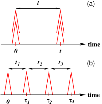
Figure 1: Schematic illustrations of the time configuration of the four-point correlation function; (a) four-point correlation function denoting the correlation of fluctuations in the two-point correlation function between two times $0$ and $t$, and (b) the three-time correlation function with correlations at four times $0$, $\tau_{1}$, $\tau_{2}$, and $\tau_{3}$.

The four-point correlation function defined by Eq. (1) is a one-time correlation function, as is schematically illustrated in Fig. 1(a). In order to quantify the temporal details of the DH and its lifetime $\tau_{\rm hetero}$, it is essential to analyze how the correlated particle motions decay with time. This requires a multi-time extension of the four-point correlation function. In practice, by following Fig. 1(b), the four-point correlation for the density field $\rho(\mbox{\boldmath$k$},t)$ can be generalized to the three-time correlation function with correlations at times $0$, $\tau_{1}$, $\tau_{2}$, and $\tau_{3}$ given by

$$F_{4}(k_{1},k_{3},t_{1},t_{2},t_{3})\\ =\langle\rho(\mbox{\boldmath$k$}_{3},\tau_{3})\rho(-\mbox{\boldmath$k$}_{3},\tau_{2})\rho(\mbox{\boldmath$k$}_{1},\tau_{1})\rho(-\mbox{\boldmath$k$}_{1},0)\rangle.$$ (3)

This equation takes into account three time intervals, $t_{1}$, $t_{2}$, and $t_{3}$. The definition of the time interval $t_{i}$ is $t_{i}=\tau_{i}-\tau_{i-1}$, where $\tau_{0}=0$.

We can define the following function as the difference between the four-point and three-time correlation function, $F_{4}(k_{1},k_{3},t_{1},t_{2},t_{3})$, and the product of the two-point correlation functions:

$$\Delta F(k_{1},k_{3},t_{1},t_{2},t_{3})\\ =F_{4}(k_{1},k_{3},t_{1},t_{2},t_{3})-F(k_{3},t_{3})F(k_{1},t_{1}).$$ (4)

This can be regarded as a multi-time extension of Eq. (1). If the dynamics are homogeneous and if the motions between the two intervals $t_{1}$ and $t_{3}$ are uncorrelated and decoupled, then the three-time correlation function $\Delta F_{4}$ should become zero. On the other hand, if the dynamics become heterogeneous, the dichotomy between the mobile and immobile regions would lead to finite values of $\Delta F_{4}$ because of the correlated motions between the two intervals $t_{1}$ and $t_{3}$. Furthermore, the progressive changes in the second time interval $t_{2}=\tau_{3}-\tau_{2}$ of $\Delta F_{4}$ enable us to investigate how the correlated motions between two time intervals $t_{1}$ and $t_{3}$ decay with the waiting time $t_{2}$. This can provide the temporal information regarding the DH that is relevant in the quest to quantify its lifetime, $\tau_{\rm hetero}$. Kim2009Multiple

Some computational studies have already utilized multi-time correlations to examine the heterogeneous dynamics. Heuer1997Heterogeneous ; Heuer1997Information ; Yamamoto1998Heterogeneous ; Doliwa1998Cage ; Perera1999Relaxation ; Qian2000Exchange ; Doliwa2002How ; Flenner2004Lifetime ; Leonard2005Lifetime However, in these calculations, only limited information has resulted (for example, results for $t_{1}=t_{3}=\tau_{\alpha}$ has been successfully provided). This lack of results has caused the aforementioned controversy regarding the temporal information that is relevant to the DH. Throughout this paper, we present the comprehensive numerical results of a four-point, three-time density correlation function without fixing any time intervals. This multi-time correlation function is used to quantify the lifetime of the DH, $\tau_{\rm hetero}$ and to determine its temperature dependence.

It is of interest to note that the multi-time correlation function can be regarded as an analogue of the nonlinear response functions of a molecular polarizability and dipoles as analyzed using the multidimensional spectroscopies such as 2D Raman spectroscopy and infrared (IR) spectroscopy. Mukamel1999Principles ; Fayer2001Ultrafast ; Khalil2003Coherent ; Tanimura2006Stochastic ; Hochstrasser2007Twodimensional ; Cho2008Coherent There exist promising theoretical treatments for the multi-time correlation function based on the mode-coupling theory. Denny2001Modecoupling ; VanZon2001Modecoupling These techniques have now become powerful and standard tools to study condensed phase dynamics. For example, there are often used to study the ultrafast dynamics of liquid water. Asbury2004Water ; Scimidt2005Pronounced ; Loparo2006Multidimensional2 ; Kraemer2008Temperature ; Paarmann2008Probing ; GarrettRoe2008Threepoint ; Yagasaki2008Ultrafast ; Yagasaki2009Molecular The utility of these techniques is enabled by the ability of the nonlinear response function to reveal details about the couplings between motions. This information is not available in the one-time linear response function. The present study analogously employs the underlying strategies and concepts of these multidimensional spectroscopy techniques to study the heterogeneous dynamics of the glass transition.

It should be remarked that unique experiments have been recently proposed to examine heterogeneous dynamics in various chemical systems, which are referred to as 2D Fourier imaging correlation spectroscopy Senning2009Kinetic and multiple population period transition spectroscopy. VanVeldhoven2007Time ; Khurmi2008Parallels These techniques provide information based on four-point correlation functions, which are basically the same as Eqs. 3 and 4.

III simulation model and some dynamical considerations

III.1 Model

We carried out MD simulations for a three-dimensional binary mixture. Our system consists of $N_{1}=500$ particles of component 1 and $N_{2}=500$ particles of component 2. They interact via a soft-core potential

$$v_{ab}(r)=\epsilon\left(\frac{\sigma_{ab}}{r}\right)^{12},$$ (5)

where

$$\sigma_{ab}=\frac{\sigma_{a}+\sigma_{b}}{2},$$ (6)

and $a,b\in\{1,2\}$. The interaction was truncated at $r=3\sigma_{1}$. The size and mass ratios were $\sigma_{1}/\sigma_{2}=1/1.2$ and $m_{1}/m_{2}=1/2$, respectively. The total number density was fixed at $\rho=N_{1}+N_{2}/L^{3}=0.8\sigma_{1}^{-3}$, where the system length was $L=10.77\sigma_{1}$ under periodic boundary conditions. In this paper, numerical results will be presented in terms of reduced units $\sigma_{1}$, $\epsilon/k_{B}$, $\tau=\sqrt{m_{1}\sigma_{1}^{2}/\epsilon}$ for length, temperature, and time, respectively. The velocity Verlet algorithm was used with a time step of $0.005\tau$ in the microcanonical ensemble. The states investigated here were $T=0.772,0.473,0.352,0.306$, and $0.289$. Below, we present and summarize the key numerical results regarding the dynamic properties of the glassy dynamics. Other information regarding this model, in particular static properties such as static structure factors can be found in some previous works. Yamamoto1998Dynamics ; Kim2000Apparent

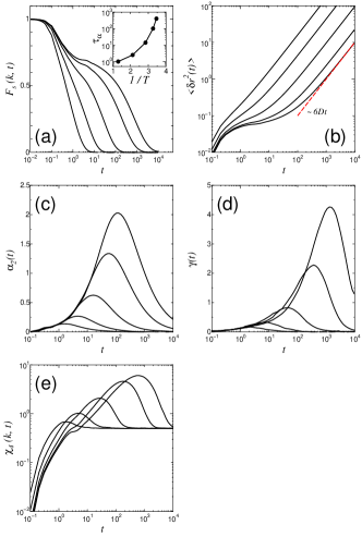
Figure 2: Time correlation functions of glass-forming liquids at temperatures $T=0.772$, $0.473$, $0.352$, $0.306$, and $0.289$ from left to right; (a) the self-part of the intermediate scattering function $F_{s}(k,t)$ with $k=2\pi$, (b) the mean square displacement $\langle\delta r^{2}(t)\rangle$, (c) the non-Gaussian parameter $\alpha_{2}(t)$, (d) the new non-Gaussian parameter $\gamma(t)$, and (e) the four-point dynamical susceptibility $\chi_{4}(k,t)$ with $k=2\pi$. Inset of (a): $\alpha$-relaxation time $\tau_{\alpha}$ as a function of the inverse temperature $1/T$. The dotted line in (b) refers to the diffusion asymptote $6Dt$ at $T=0.289$.

III.2 Intermediate scattering function and mean square displacement

To begin, we examined the density fluctuation in terms of the self-part of the intermediate scattering function of component $1$ particles that is defined as

$$F_{s}(k,t)=\left\langle\frac{1}{N_{1}}\sum_{j=1}^{N_{1}}\exp[i\mbox{\boldmath$k$}\cdot\Delta\mbox{\boldmath$r$}_{j}(0,t)]\right\rangle,$$ (7)

where $\Delta\mbox{\boldmath$r$}_{j}(0,t)\equiv\mbox{\boldmath$r$}_{j}(t)-\mbox{\boldmath$r$}_{j}(0)$ is the $j$th particle displacement vector during the two times $0$ and $t$. The behavior of $F_{s}(k,t)$ is often utilized to study the non-exponential decay of the structural relaxation as demonstrated in Fig. 2(a). Here the wave vector is chosen as $k=2\pi$. This corresponds to the wave vector of the first peak of the static structure factor. Also well known is the fact that when the temperature decreases, this function plateaus during the $\beta$-relaxation regime. In this regime, a tagged particle is trapped by its surrounding caged particles. Eventually, the tagged particle escapes from the cage on a much longer time scale, which is referred to as the $\alpha$-relaxation regime. In this paper, we define the $\alpha$-relaxation time $\tau_{\alpha}$ as $F_{s}(k,\tau_{\alpha})=e^{-1}$ with $k=2\pi$. In the inset of Fig. 2(a), the temperature dependence of $\tau_{\alpha}$ is plotted as a function of the inverse of the temperature $1/T$. We observe that the structural $\alpha$-relaxation time is drastically increased and exhibits super-Arrhenius behavior as the temperature is decreased.

Particle motions are also analyzed through the mean square displacement (MSD). We calculated the MSD for the particles of component $1$,

$$\langle\delta r^{2}(t)\rangle=\left\langle\frac{1}{N_{1}}\sum_{j=1}^{N_{1}}|\Delta\mbox{\boldmath$r$}_{j}(0,t)|^{2}\right\rangle,$$ (8)

and displayed the results in Fig. 2(b) for various temperature. As shown in Fig. 2(b), at lower temperatures a plateau develops during the intermediate $\beta$-relaxation regime, when the cage effect is dominant. Diffusive behavior, $\langle\delta r^{2}(t)\rangle=6Dt$ , eventually sets in over the time scale of $t\simeq\tau_{\alpha}$.

III.3 Non-Gaussian parameter

We next employ the non-Gaussian parameter (NGP) $\alpha_{2}(t)$ defined as

$$\alpha_{2}(t)=\frac{3\langle\delta r^{4}(t)\rangle}{5\langle\delta r^{2}(t)\rangle^{2}}-1,$$ (9)

with $\langle\delta r^{4}(t)\rangle=\langle(1/N_{1})\sum_{j=1}^{N_{1}}|\Delta\mbox{\boldmath$r$}_{j}(0,t)|^{4}\rangle$. The $\alpha_{2}(t)$ reveals how the distribution of the single-particle displacement, $\delta r$, at time $t$ deviates away from the Gaussian distribution. Hansen2006Theory As is well documented Kob1997Dynamical and shown in Fig. 2(c), $\alpha_{2}(t)$ begins to grow as the temperature is decreased. The growth of $\alpha_{2}(t)$ means that the distribution of the displacement will have two peaks. These peaks indicate the existence of both mobile and immobile particles, the main feature of DH. However, it is noted that $\alpha_{2}(t)$ mainly grows in the $\beta$-relaxation regime, when the $F_{s}(k,t)$ plateaus (see Fig. 2(a)). In practice, in the time scales at the beginning of the $\beta$-relaxation regime, $\alpha_{2}(t)$ begins to grow, whereas on the time scale of $\tau_{\alpha}$, $\alpha_{2}(t)$ begins to decrease to zero. This is due to the fact that $\alpha_{2}(t)$ is strongly dominated by the mobile particles which move faster than particles with a Gaussian distribution. The time $\tau_{\rm NGP}$ during $\alpha_{2}(t)$ has a peak thus becomes smaller than $\tau_{\alpha}$ at lower temperatures. It is remarked that a similar behavior in $\alpha_{2}(t)$ has been demonstrated using the mode-coupling theory, which incorporates hopping motions. Chong2008Connections

Instead of using the NGP $\alpha_{2}(t)$, Flenner and Szamel have recently proposed a new non-Gaussian parameter (NNGP), $\gamma(t)$, defined as

$$\gamma(t)=\frac{1}{3}\langle\delta r^{2}(t)\rangle\left\langle\frac{1}{\delta r^{2}(t)}\right\rangle-1,$$ (10)

with $\langle 1/\delta r^{2}(t)\rangle=\langle(1/N_{1})\sum_{j=1}^{N_{1}}|\Delta\mbox{\boldmath$r$}_{j}(0,t)|^{-2}\rangle$. The $\gamma(t)$ strongly weights the immobile particles which have not move as far as the Gaussian distribution would predict. Flenner2005RelaxationBD Figure 2(d) demonstrates $\gamma(t)$ for various temperatures. It is observed that the time $\tau_{\rm NNGP}$ at which $\gamma(t)$ has a peak is of a longer time scale than $\tau_{\alpha}$. This is in contrast to the results of the conventional NGP analysis as shown in Fig. 2(c).

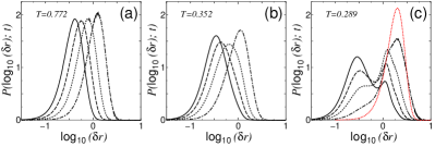
Figure 3: Distribution of the logarithm of the single-particle displacement $P(\log_{10}(\delta r);t)$ at $T=0.772$ (a), $0.352$ (b), and $0.289$ (b). For each temperature, the times shown are $t=\tau_{\alpha}$ (solid curve), $2\tau_{\alpha}$ (dashed curve), $4\tau_{\alpha}$ (short dashed curve), and $10\tau_{\alpha}$ (dash-dotted curve). The dotted curve in (c) refers to the Gaussian distribution $G_{s}(\delta r,t)=[1/(4\pi Dt)^{3/2}]\exp(-\delta r^{2}/4Dt)$ at $t=10\tau_{\alpha}$, where the diffusion constant $D$ is evaluated by the asymptote $6Dt$ of the mean squared displacement (see Fig. 2(b)).

III.4 Four-point dynamical susceptibility

As mentioned in Sec. II.1, the four-point correlation function that is defined as the correlation function of the fluctuations in the two-point correlation functions has become a powerful tool to determine the correlation length of the DH. Although there are several definitions for $\chi_{4}(k,t)$, one is given by, Szamel2006Four

$$\chi_{4}(k,t)=N_{1}\left\langle\left[\frac{1}{N_{1}}\sum_{j=1}^{N_{1}}\delta F_{j}(\mbox{\boldmath$k$},0,t)\right]^{2}\right\rangle,$$ (11)

where

$$\delta F_{j}(\mbox{\boldmath$k$},0,t)=\cos[\mbox{\boldmath$k$}\cdot\Delta\mbox{\boldmath$r$}_{j}(0,t)]-F_{s}(k,t),$$ (12)

represents the individual fluctuations in the real-part and self-part of the intermediate scattering function between time $0$ and time $t$. Alternatively, $\chi_{4}(k,t)$ can be expressed by Toninelli2005Dynamical

$$\chi_{4}(k,t)=N_{1}[\langle\hat{F}_{s}(\mbox{\boldmath$k$},t)^{2}\rangle-\langle\hat{F_{s}}(\mbox{\boldmath$k$},t)\rangle^{2}].$$ (13)

Here we adopt $\hat{F}_{s}(\mbox{\boldmath$k$},t)$ as

$$\hat{F}_{s}(\mbox{\boldmath$k$},t)=\frac{1}{N_{1}}\sum_{j=1}^{N_{1}}\cos[\mbox{\boldmath$k$}\cdot\Delta\mbox{\boldmath$r$}_{j}(0,t)],$$ (14)

with $F_{s}(k,t)=\langle\hat{F}_{s}(\mbox{\boldmath$k$},t)\rangle$. The $\chi_{4}(k,t)$ shows the correlation of the fluctuation in the two-point correlation function $F_{s}(k,t)$. This reveals how the particle motions (or trajectories) between times $0$ and $t$ are correlated. In other words, the amplitude of $\chi_{4}(k,t)$ signals the total amount of spatial correlations in the particle displacements within the given time interval $t$. As seen in Fig. 2(e), the $\chi_{4}(k,t)$ typically presents non-monotonic time behavior. The peak of $\chi_{4}(k,t)$ appears on a time scale that is comparable to $\tau_{\alpha}$. Note that the ensemble dependence of the dynamical susceptibility is not taken into account since the microcanonical dynamics is employed in our simulations.

III.5 Distribution of single-particle displacements

We end this section with a discussion of the distribution of single-particle displacements, as alluded to above. Following Flenner and Szamel, Flenner2005RelaxationBD we calculated the distribution $P(\log_{10}(\delta r);t)$ of the logarithm of the particle displacements, $\delta r$, at time $t$. These displacements are obtained from the self-part of the van-Hove correlation function $G_{s}(\delta r,t)$ as

$$P(\log_{10}(\delta r);t)=\ln(10)4\pi\delta r^{3}G_{s}(\delta r,t).$$ (15)

Figure 3 shows $P(\log_{10}(\delta r);t)$ at various times $t$ for $T=0.772$, $0.352$, and $0.289$. The dotted red curve in Fig. 3(c) refers to the distribution of the Gaussian process, $G_{s}(\delta r,t)=[1/(4\pi Dt)^{3/2}]\exp(-\delta r^{2}/4Dt)$ with the diffusion constant $D$ at $T=0.289$. It is noted here that the Gaussian distribution is independent of time $t$, and the peak height is given by $P(\log_{10}(\delta r);t)\approx 2.13$. Flenner2005RelaxationBD At the high temperature $T=0.772$, there is only one peak during time $t$. This peak has the smallest deviation from the Gaussian distribution. On the contrary, at the lowest temperature $T=0.289$, we clearly see the two distinct mobile and immobile peaks. These peaks clearly have large deviations from the Gaussian even for longer time scales than $\tau_{\alpha}$, implying the long-lived DH. Szamel2006Time

IV numerical results of the multi-time correlation function

IV.1 Three-time density correlation function

Following the time configuration illustrated in Fig. 1(b) and Eq. (4), we extend the dynamical susceptibility $\chi_{4}(k,t)$ defined by Eq. (11) to the three-time density correlation function with times $0$, $\tau_{1}$, $\tau_{2}$, and $\tau_{3}$. This is defined as

$$\Delta F_{4}(k,t_{1},t_{2},t_{3})\\ =\biggl{\langle}\frac{1}{N_{1}}\sum_{j=1}^{N_{1}}\delta F_{j}(\mbox{\boldmath$k$},\tau_{2},\tau_{3})\delta F_{j}(\bm{k},0,\tau_{1}))\biggr{\rangle}.$$ (16)

We note that Eq. (16) is regarded as the self-part of Eq. (4). Moreover, the wave vector is chosen as $k=k_{1}=k_{3}$ in our numerical calculations. As discussed in Sec. II.2, $\Delta F_{4}(k,t_{1},t_{2},t_{3})$ denotes the correlations of fluctuations in the two-point correlation function $F_{s}(k,t)$ between two time intervals, $t_{1}=\tau_{1}$ and $t_{3}=\tau_{3}-\tau_{2}$.

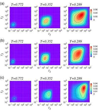
Figure 4: 2D representations of the three-time correlation functions; (a) total $\Delta F_{4}(k,t_{1},t_{2},t_{3})$, (b) the mobile part $\Delta F_{4}^{\rm mo}(k,t_{1},t_{2},t_{3})$, and (c) the immobile part $\Delta F_{4}^{\rm im}(k,t_{1},t_{2},t_{3})$ at waiting time $t_{2}=0$ for various temperatures $T=0.772$, $0.352$, and $0.289$ from left to right. The wave vector $k$ is chosen as $k=2\pi$.

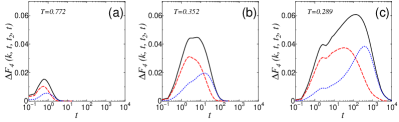
Figure 5: Diagonal parts of the three-time correlation functions, $\Delta F_{4}$, $\Delta F_{4}^{\rm mo}$, and $\Delta F_{4}^{\rm im}$ at waiting time $t_{2}=0$ for $T=0.772$ (a) $0.352$ (b), and $0.289$ (c). The solid, dashed, and short dashed curves correspond to total, mobile, and immobile parts, respectively.

Furthermore, the three-time correlation function given by Eq. (16) can be divided into two parts as

$$\Delta F_{4}(k,t_{1},t_{2},t_{3})\\ =\Delta F_{4}^{\rm mo}(k,t_{1},t_{2},t_{3})+\Delta F_{4}^{\rm im}(k,t_{1},t_{2},t_{3}),$$ (17)

where $\Delta F_{4}^{\rm mo}$ ($\Delta F_{4}^{\rm im}$) represents the mobile (immobile) part, arising from the contribution of mobile (immobile) particles during the first time interval, $t_{1}$. Practically, we defined the mobile (immobile) particles as those particles that move more (less) than the mean value of the single-particle displacement, $\sqrt{\langle\delta r^{2}(t_{1})\rangle}$, for the first time interval $t_{1}$. During $t_{1}$, the function $\delta F_{j}(\mbox{\boldmath$k$},0,\tau_{1})$ selects the sub-ensemble of mobile (immobile) contributions in the DH, and the total function $\delta F_{j}(\mbox{\boldmath$k$},\tau_{2},\tau_{3})\delta F_{j}(\mbox{\boldmath$k$},0,\tau_{1})$ contains information to determine how long the mobile (immobile) particles remain during the waiting time $t_{2}$. This information gained from the three-time correlation function $\Delta F_{4}$ is related to the joint probability $P(\delta r(t_{3})|\delta r(t_{1}))$ of two successive particle displacements, $\delta r(t_{3})$ and $\delta r(t_{1})$. This joint probability describes the probability of the particle being mobile (immobile) at $t_{1}$ and remaining mobile (immobile) at $t_{3}$ after the waiting time $t_{2}$. More details will be given elsewhere by analyzing the multi-time correlation functions of the particle displacements. Kim2010preparation

IV.2 Zero waiting time $t_{2}=0$

We first present the numerical results of the three-time density correlation function, $\Delta F_{4}(k,t_{1},t_{2},t_{3})$, at the waiting time $t_{2}=0$. These are shown in Fig. 4(a) at various temperatures, $T=0.772$, $0.352$, and $0.289$. It can be seen that the intensity of $\Delta F_{4}(k,t_{1},t_{2},t_{3})$ gradually grows with decreasing the temperature. This indicates that particles that are mobile (immobile) during the first time interval, $t_{1}$, tend to remain mobile (immobile) during the subsequent time interval, $t_{3}$. It can also be seen that the profile of $\Delta F_{4}(k,t_{1},t_{2},t_{3})$ is widely broadened, suggesting that the motions between various time scales, including $\alpha$- and $\alpha$-relaxation and $\alpha$- and $\beta$-relaxation, are coupled. Furthermore, the time at which $\Delta F_{4}$ has its maximum value is approximately given by the $\alpha$-relaxation time, $\tau_{\alpha}$.

To describe the details of $\Delta F_{4}(k,t_{1},t_{2},t_{3})$ more fully, we show the mobile and immobile parts of the system, $\Delta F_{4}^{\rm mo}(k,t_{1},t_{2},t_{3})$ and $\Delta F_{4}^{\rm im}(k,t_{1},t_{2},t_{3})$ in Fig. 4(b) and (c), respectively. These diagonal parts at $t_{1}=t_{3}$ are also drawn in Fig. 5 for $T=0.772$ (a), $0.352$ (b), and $0.289$ (c). It can be seen that the peak of $\Delta F_{4}$ is composed of the two distinct mobile and immobile contributions particularly at the lower temperatures. The time scales of the two contributions are different, i.e., the peak of the mobile part, $\Delta F_{4}^{\rm mo}$, appears at $t_{1}\simeq\tau_{\rm NGP}$, while the peak of the immobile part, $\Delta F_{4}^{\rm mo}$, is pronounced on the time scale of $t_{1}\simeq\tau_{\rm NNGP}$. These findings are expected as per the discussion in Sec. III.3. Specifically, the NGP focuses on the mobile particles and the NNGP weights the immobile contributions of the non-Gaussian distribution of the particle displacement (see Fig. 3(c)).

IV.3 Waiting time $t_{2}$ dependence and the lifetime of the dynamical heterogeneity

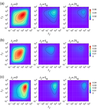
Figure 6: 2D representations of the three-time correlation functions; (a) total $\Delta F_{4}(k,t_{1},t_{2},t_{3})$, (b) the mobile part $\Delta F_{4}^{\rm mo}(k,t_{1},t_{2},t_{3})$, and (c) the immobile part $\Delta F_{4}^{\rm im}(k,t_{1},t_{2},t_{3})$ at $T=0.289$. Waiting times are varied for $t_{2}=0$, $\tau_{\alpha}$, and $3\tau_{\alpha}$ from left to right. The wave vector $k$ is chosen as $k=2\pi$.

As outlined in Sec. II.2, the progressive changes in the waiting time $t_{2}=\tau_{3}-\tau_{2}$ of the three-time correlation function $\Delta F_{4}(k,t_{1},t_{2},t_{3})$ make it possible to investigate how the correlated motions decay with time. Figure 6 shows the time evolutions of the three-time correlation functions, $\Delta F_{4}$, $\Delta F_{4}^{\rm mo}$, and $\Delta F_{4}^{\rm im}$ at the lowest temperature of $T=0.289$. We also plot the diagonal parts of the evolution along $t_{1}=t_{3}$ at various $t_{2}$ in Fig. 7. It is demonstrated that the correlations gradually decay as the waiting time $t_{2}$ increases. The values of the three-time correlation functions tend toward zero for $t_{2}\to\infty$. We also find that for larger $t_{2}$, the peak of $\Delta F_{4}$ tends to shift to $t\simeq 1000$, which is close to $\tau_{\rm NNGP}$. This peak shift is attributed to the fact that immobile particles tend to remain immobile on larger time scales as indicated in Fig. 6(c). Moreover, the presence of correlations on larger time scales than the $\alpha$-relaxation time scale is observed, even for $t_{2}=10\tau_{\alpha}$. It is also clearly seen that the off-diagonal parts of $\Delta F_{4}$, $\Delta F_{4}^{\rm mo}$, and $\Delta F_{4}^{\rm im}$ become noticeable with increasing $t_{2}$. These observations imply that the relaxation rates of $\Delta F_{4}$, $\Delta F_{4}^{\rm mo}$, and $\Delta F_{4}^{\rm im}$ largely depend on which time scale is examined.

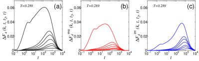
Figure 7: Diagonal parts of the three-time correlation functions; (a) total $\Delta F_{4}$, (b) the mobile $\Delta F_{4}^{\rm mo}$, and (c) the immobile $\Delta F_{4}^{\rm im}$ at $T=0.289$. Waiting times are varied at $t_{2}=0$, $0.5\tau_{\alpha}$, $\tau_{\alpha}$, $2\tau_{\alpha}$, $4\tau_{\alpha}$, $6\tau_{\alpha}$, and $10\tau_{\alpha}$ from top to bottom.

To explore the details of the time scale of the correlated motions, we define the relaxation time $\hat{\tau}_{\rm hetero}(t_{1},t_{3})$ of the $\Delta F_{4}(k,t_{1},t_{2},t_{3})$ as

$$\Delta F_{4}(k,t_{1},\hat{\tau}_{\rm hetero},t_{3})/\Delta F_{4}(k,t_{1},0,t_{3})=e^{-1},$$ (18)

for various values of $t_{1}$ and $t_{3}$. Similarly, the relaxation times $\hat{\tau}_{\rm hetero}^{\rm mo}(t_{1},t_{3})$ and $\hat{\tau}_{\rm hetero}^{\rm im}(t_{1},t_{3})$ are determined from $\Delta F_{4}^{\rm mo}$ and $\Delta F_{4}^{\rm im}$, respectively. Figure 8 shows the 2D representations of the relaxation times $\hat{\tau}_{\rm hetero}$, $\hat{\tau}_{\rm hetero}^{\rm mo}$, and $\hat{\tau}_{\rm hetero}^{\rm im}$ at $T=0.289$. We confirm that the relaxation time $\hat{\tau}_{\rm hetero}$ of the total function $\Delta F_{4}$ is described by the summation of the mobile and immobile parts, $\hat{\tau}_{\rm hetero}^{\rm mo}$ and $\hat{\tau}_{\rm hetero}^{\rm im}$. Furthermore, it is of interest to note that the distribution of the $\hat{\tau}_{\rm hetero}$ has a multiple structure; the relaxation time $\hat{\tau}_{\rm hetero}$ becomes much larger than the time scale, $\tau_{\alpha}$, if the time interval $t_{1}$ or the time interval $t_{3}$ is examined for larger time scale than $\tau_{\alpha}$. On the other hand, $\hat{\tau}_{\rm hetero}$ becomes smaller than $\tau_{\alpha}$ if $t_{1}$ or $t_{3}$ is examined for smaller time scale than $\tau_{\alpha}$.

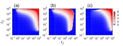
Figure 8: 2D representations of relaxation time distributions of three-time correlation functions; (a) $\hat{\tau}_{\rm hetero}$, (b) $\hat{\tau}_{\rm hetero}^{\rm mo}$, and (c) $\hat{\tau}_{\rm hetero}^{\rm im}$. normalized by $\tau_{\alpha}$ at $T=0.289$. The dotted line refers to the iso-line of $\tau_{\rm hetero}=\tau_{\alpha}$ in each panel.

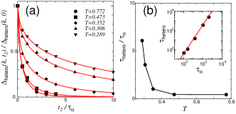
Figure 9: (a) Waiting time $t_{2}$ dependence of the integrated three-time correlation function $\Delta_{\rm hetero}(k,t_{2})/\Delta_{\rm hetero}(k,0)$ with $k=2\pi$ for various temperatures. The waiting times are normalized by $\tau_{\alpha}$ for each temperature. The solid curve is determined by a fitting with the stretched-exponential form for each temperature. (b) Average lifetime of DH $\tau_{\rm hetero}$ normalized by the $\alpha$-relaxation $\tau_{\alpha}$ versus temperature $T$. Inset: Relation between two time scales, $\tau_{\rm hetero}$ and $\tau_{\alpha}$. The straight line with the slope 1.5 is presented as a viewing guide.

In order to obtain the average lifetime of the DH, we define the volume of the heterogeneities as

$$\Delta_{\rm hetero}(k,t_{2})=\int_{0}^{\infty}dt_{3}\int_{0}^{\infty}dt_{1}\Delta F_{4}(k,t_{1},t_{2},t_{3}).$$ (19)

We examined the $t_{2}$ dependence of $\Delta_{\rm hetero}(k,t_{2})$. Figure 9(a) shows $\Delta_{\rm hetero}(k,t_{2})/\Delta_{\rm hetero}(k,0)$ as a function of the waiting time $t_{2}$ normalized by $\tau_{\alpha}$ at each temperature. From Fig. 9(a), we see that $\Delta_{\rm hetero}$ rapidly decays to zero at higher temperatures and that the time scale is comparable to $\tau_{\alpha}$. In contrast, at lower temperatures, the relaxation of $\Delta_{\rm hetero}$ occurs on a time scale larger than $\tau_{\alpha}$. $\Delta_{\rm hetero}(k,t_{2})/\Delta_{\rm hetero}(k,0)$ can be fitted by the stretched-exponential function $\exp[-(t_{2}/\tau_{\rm hetero})^{c}]$, where $\tau_{\rm hetero}$ can be regarded as the average lifetime of the DH. We obtain the approximate relation as $\tau_{\rm hetero}\simeq\int\int\hat{\tau}_{\rm hetero}(t_{1},t_{3})dt_{1}dt_{3}/\int\int dt_{1}dt_{3}$. We plot $\tau_{\rm hetero}$ at each temperature $T$ in Fig. 9(b). It is found in Fig. 9(b) that $\tau_{\rm hetero}$ becomes much larger than $\tau_{\alpha}$ as the temperature $T$ decreases. In practice, the lifetime $\tau_{\rm hetero}$ is approximately $6\tau_{\alpha}\simeq 2400$ with $c\simeq 0.5$ at the lowest temperature of $T=0.289$. Furthermore, as seen in the inset of Fig. 9(b), we observe the strong deviation between the two time scales $\tau_{\rm hetero}$ and $\tau_{\alpha}$ that follows the power low, $\tau_{\rm hetero}\sim{\tau_{\alpha}}^{1.5}$. Similarly, we determined the average lifetimes $\tau_{\rm hetero}^{\rm mo}$ and $\tau_{\rm hetero}^{\rm im}$ for the mobile and immobile parts. We confirm that $t_{2}$ dependences of the mobile and immobile parts are close to that of the total function and that $\tau_{\rm hetero}^{\rm mo}$ and $\tau_{\rm hetero}^{\rm im}$ are comparable to $\tau_{\rm hetero}$ for each temperature (data not shown).

IV.4 2D spectra of three-time correlation functions

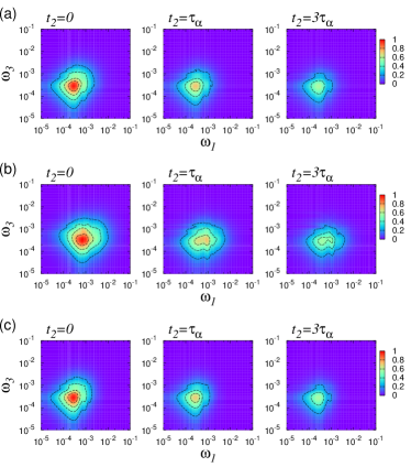
Figure 10: Imaginary parts of 2D spectra of the three-time correlation functions; (a) total $\Im[\Delta F_{4}(k,\omega_{1},t_{2},\omega_{3})]$, (b) the mobile part $\Im[\Delta F_{4}^{\rm mo}(k,\omega_{1},t_{2},\omega_{3})]$, and (c) the immobile part $\Im[\Delta F_{4}^{\rm im}(k,\omega_{1},t_{2},\omega_{3})]$ at $T=0.289$. Waiting times are varied at $t_{2}=0$, $\tau_{\alpha}$, and $3\tau_{\alpha}$ from left to right. The wave vector $k$ is chosen as $k=2\pi$. The profile is normalized by the peak value at $t_{2}=0$ for each panel.

Through the use of the analogy to the 2D IR spectroscopy, it is of interest to examine the three-time correlation function $\Delta F_{4}(k,t_{1},t_{2},t_{3})$ in the frequency domain. The Fourier transformed 2D spectrum is obtained by

$$\Delta F_{4}(k,\omega_{1},t_{2},\omega_{3})\\ =\int_{0}^{\infty}dt_{3}\int_{0}^{\infty}dt_{1}\Delta F_{4}(k,t_{1},t_{2},t_{3})e^{i\omega_{1}t_{1}+i\omega_{3}t_{3}}.$$ (20)

Similarly, the mobile part $\Delta F_{4}^{\rm mo}$ and immobile part $\Delta F_{4}^{\rm im}$ can be represented in the frequency domain with respect to $t_{1}$ and $t_{3}$. In Fig. 10, we present the imaginary parts of 2D spectra, the total $\Im[\Delta F_{4}(k,\omega_{1},t_{2},\omega_{3})]$ (a), the mobile part $\Im[\Delta F_{4}^{\rm mo}(k,\omega_{1},t_{2},\omega_{3})]$ (b), and the immobile part $\Im[\Delta F_{4}^{\rm im}(k,\omega_{1},t_{2},\omega_{3})]$ (c) at $T=0.289$ for several waiting times. It is seen in Fig. 10(a) that the peak of $\Im[\Delta F_{4}]$ appears near the detected slower time scale, $(\omega_{1},\omega_{3})\simeq(\tau_{\rm hetero}^{-1},\tau_{\rm hetero}^{-1})$, which is longer-lived for larger waiting times. The peak is diagonally elongated at $t_{2}=0$ because of the strong correlations between two the frequencies $\omega_{1}$ and $\omega_{3}$. The elongation that is directed toward the high frequency side tends to be lost because of the loss of the frequency correlations at larger $t_{2}$. Moreover, the off-diagonal cross peaks become pronounced at $(\omega_{1},\omega_{3})\simeq(\tau_{\rm NNGP}^{-1},\tau_{\rm hetero}^{-1})$ and $(\tau_{\rm hetero}^{-1},\tau_{\rm NNGP}^{-1})$. The time scale $\tau_{\rm NNGP}$ corresponds to the peak position of $\Delta F_{4}(k,t_{1},t_{2},t_{3})$ at larger $t_{2}$, as seen in Fig. 6(a).

Similar behaviors are observed in the 2D spectra of the mobile and immobile parts, $\Im[\Delta F_{4}^{\rm mo}]$ and $\Im[\Delta F_{4}^{\rm im}]$. The mobile part $\Im[\Delta F_{4}^{\rm mo}]$ is rather horizontally elongated until $\omega_{1}\simeq\tau_{\rm NGP}^{-1}$ because of the coupling between $\omega_{3}\simeq\tau_{\rm hetero}^{-1}$ and the higher frequency $\omega_{1}$, which is correlated to the 2D representation in the time domain that is seen in Fig. 6(b). Furthermore, the immobile part $\Im[\Delta F_{4}^{\rm im}]$ tends to be almost symmetric for the diagonal line $\omega_{1}=\omega_{3}$, although the 2D profile in time domain is largely asymmetric as seen in Fig. 6(c).

V conclusions and final remarks

We have investigated the four-point, three-time density correlation function to quantitatively characterize the temporal structures of the DH. The correlations detected by the three-time correlation function can be divided into two parts, mobile and immobile contributions determined from the single-particle displacement during the first time interval. These 2D representations in both the time and frequency domains that are presented over a wide range of time scales enable us to explore the couplings of particle motions. It is shown that the peak positions of the mobile and immobile parts are correlated to the dominant time scales of the non-Gaussian parameters. These extracted results are not obtainable from a one-time correlation function.

Furthermore, the progressive changes in the waiting time allow us to obtain detailed information regarding the correlations of motions decay with the time. The waiting time dependence of the multi-time correlation function shows the existence of the correlations on larger time scales between immobile particles. The multi-time correlations allow for the quantification of the average lifetime of the DH, $\tau_{\rm hetero}$, in glass-forming liquids. Our analysis can be regarded as an analogue of the multidimensional nonlinear spectroscopic analysis applied to liquids and biological systems to understand ultrafast dynamics, e.g., the transition from inhomogeneous to homogeneous broadening and the couplings between molecular motions.

We have found that the $\tau_{\rm hetero}$ becomes much slower than the $\alpha$-relaxation time $\tau_{\alpha}$ when the system is highly supercooled. This is due to the long-lived DH at lower temperatures. Our findings show that the presence of the new time scale $\tau_{\rm hetero}$ exceeds that of the $\alpha$-relaxation time, $\tau_{\alpha}$. These findings are correlated with recent numerical studies. Yamamoto1998Heterogeneous ; Leonard2005Lifetime ; Szamel2006Time ; Hedges2007Decoupling ; Kawasaki2009Apparent ; Tanaka2010Criticallike ; Mizuno2010Life Such strong deviations and decouplings between $\tau_{\rm hetero}$ and $\tau_{\alpha}$ when approaching the glass transition temperature have been observed in some experiments, Wang1999How ; Wang2000Lifetime in which the lifetime of a sub-ensemble is measured after selective excitation. Recent single-molecule experiments that detect the local mobility of probe molecules dispersed in glassy materials have other relevance to our simulations Deschenes2002Heterogeneous ; Adhikari2007Heterogeneous ; Zondervan2007Local ; Mackowiak2009Spatial . In these experiments, the lifetime of the dynamical heterogeneity is evaluated from the exchange time between mobile and immobile regions, which is found to be much slower than the structural relaxation time $\tau_{\alpha}$ near the glass transition temperature.

It is of great importance to examine the relation between the length and time scales of the DH in order to characterize the relevant spatiotemporal structures. So far, various relations such as $\tau\sim\xi^{z}$ as seen in critical phenomena Yamamoto1998Dynamics ; Perera1999Relaxation ; Lacevic2003Spatially ; Whitelam2004Dynamic ; Stein2008Scaling or $\tau\sim\exp((\xi/k_{B}T)^{\zeta})$ based on the random first order transition Karmakar2009Growing have been proposed. In these studies, the four-point correlation function is used to extract the length scale $\xi$ of the DH, where the fluctuation in the two-point correlation function $\delta F(\mbox{\boldmath$k$},t)$ is considered as an order parameter as seen in Eq. (1). On the contrary, the time scale is typically chosen as the relaxation time of the two-point density correlation function, $\tau_{\alpha}$. Here, we show that the time scale $\tau$ associated with $\xi$ should not be $\tau_{\alpha}$ but should instead be the average lifetime of the order parameter, i.e., $\tau_{\rm hetero}$. This $\tau_{\rm hetero}$ is hidden in the two-point correlation function and unveiled when we apply the the four-point, three-time correlation function.

It is worth mentioning that several recent attempts have utilized the multi-time correlation function to detect heterogeneous dynamics. A third-order nonlinear susceptibility is theoretically applied to the glassy systems. Bouchaud2005Nonlinear ; Tarzia2010Anomalous . Recently this concept has been tested experimentally to measure the DH. CrausteThibierge2010Evidence Furthermore, as previously mentioned, recent 2D optical techniques Senning2009Kinetic ; VanVeldhoven2007Time ; Khurmi2008Parallels can in principle provide information on heterogeneous dynamics via 2D representations of multi-time correlation functions. We hope that our numerical results will be directly compared with the experimental ones in the future.

- (1) P. G. Debenedetti, Metastable Liquids (Princeton University Press, 1996).
- (2) E. Donth, The Glass Transition (Springer, 2001).
- (3) K. Binder and W. Kob, Glassy Materials and Disordered Solids (World Scientific, Singapore, 2005).
- (4) M. D. Ediger, C. A. Angell, and S. R. Nagel, J. Phys. Chem. 100, 13200 (1996).
- (5) P. G. Debenedetti and F. H. Stillinger, Nature 410, 259 (2001).
- (6) A. Cavagna, Phys. Rep. 476, 51 (2009).
- (7) K. Schmidt-Rohr and H. W. Spiess, Phys. Rev. Lett. 66, 3020 (1991).
- (8) A. Heuer, M. Wilhelm, H. Zimmermann, and H. W. Spiess, Phys. Rev. Lett. 75, 2851 (1995).
- (9) R. Böhmer, G. Hinze, G. Diezemann, B. Geil, and H. Sillescu, Europhys. Lett. 36, 55 (1996).
- (10) E. Vidal Russell and N. E. Israeloff, Nature 408, 695 (2000).
- (11) H. Sillescu, J. Non-Cryst. Solids 243, 81 (1999).
- (12) M. D. Ediger, Annu. Rev. Phys. Chem. 51, 99 (2000).
- (13) R. Richert, J. Phys.: Condens. Matter 14, R703 (2002).
- (14) M. M. Hurley and P. Harrowell, Phys. Rev. E 52, 1694 (1995).
- (15) W. Kob, C. Donati, S. J. Plimpton, P. H. Poole, and S. C. Glotzer, Phys. Rev. Lett. 79, 2827 (1997).
- (16) C. Donati, J. F. Douglas, W. Kob, S. J. Plimpton, P. H. Poole, and S. C. Glotzer, Phys. Rev. Lett. 80, 2338 (1998).
- (17) T. Muranaka and Y. Hiwatari, Phys. Rev. E 51, R2735 (1995).
- (18) R. Yamamoto and A. Onuki, Phys. Rev. E 58, 3515 (1998).
- (19) R. Yamamoto and A. Onuki, Phys. Rev. Lett. 81, 4915 (1998).
- (20) D. N. Perera and P. Harrowell, J. Chem. Phys. 111, 5441 (1999).
- (21) K. Kim and R. Yamamoto, Phys. Rev. E 61, R41 (2000).
- (22) S. C. Glotzer, J. Non-Cryst. Solids 274, 342 (2000).
- (23) B. Doliwa and A. Heuer, J. Non-Cryst. Solids 307-310, 32 (2002).
- (24) N. Lačević, F. W. Starr, T. B. Schrøder, and S. C. Glotzer, J. Chem. Phys. 119, 7372 (2003).
- (25) L. Berthier, Phys. Rev. E 69, 020201(R) (2004).
- (26) A. Widmer-Cooper and P. Harrowell, Phys. Rev. Lett. 96, 185701 (2006).
- (27) A. Widmer-Cooper, H. Perry, P. Harrowell, and D. R. Reichman, Nature Phys. 4, 711 (2008).
- (28) H. Tanaka, T. Kawasaki, H. Shintani, and K. Watanabe, Nature Mater. 9, 324 (2010).
- (29) A. H. Marcus, J. Schofield, and S. A. Rice, Physs Rev. E 60, 5725 (1999).
- (30) W. K. Kegel and A. van Blaaderen, Science 287, 290 (2000).
- (31) E. R. Weeks, J. Crocker, A. C. Levitt, A. Schofield, and D. Weitz, Science 287, 627 (2000).
- (32) E. R. Weeks and D. A. Weitz, Phys. Rev. Lett. 89, 095704 (2002).
- (33) E. R. Weeks, J. C. Crocker, and D. A. Weitz, J. Phys.: Condens. Matt. 19, 205131 (2007).
- (34) V. Prasad, D. Semwogerere, and E. R. Weeks, J. Phys.: Condens. Matt. 19, 113102 (2007).
- (35) S. Franz and G. Parisi, J. Phys.: Condens. Matt. 12, 6335 (2000).
- (36) C. Donati, S. Franz, S. C. Glotzer, and G. Parisi, J. Non-Cryst. Solids 307-310, 215 (2002).
- (37) S. Whitelam, L. Berthier, and J. P. Garrahan, Phys. Rev. Lett. 92, 185705 (2004).
- (38) C. Toninelli, M. Wyart, L. Berthier, G. Biroli, and J. P. Bouchaud, Phys. Rev. E 71, 041505 (2005).
- (39) D. Chandler, J. P. Garrahan, R. L. Jack, L. Maibaum, and A. C. Pan, Phys. Rev. E 74, 051501 (2006).
- (40) G. Szamel and E. Flenner, Phys. Rev. E 74, 021507 (2006).
- (41) H. Shintani and H. Tanaka, Nature Phys. 2, 200 (2006).
- (42) L. Berthier, G. Biroli, J. P. Bouchaud, W. Kob, K. Miyazaki, and D. R. Reichman, J. Chem. Phys. 126, 184503 (2007).
- (43) L. Berthier, G. Biroli, J. P. Bouchaud, W. Kob, K. Miyazaki, and D. R. Reichman, J. Chem. Phys. 126, 184504 (2007).
- (44) E. Flenner and G. Szamel, J. Phys.: Condens. Matter 19, 205125 (2007).
- (45) R. S. L. Stein and H. C. Andersen, Phys. Rev. Lett. 101, 267802 (2008).
- (46) S. Karmakar, C. Dasgupta, and S. Sastry, Proc. Natl. Acad. Sci. U.S.A. 106, 3675 (2009).
- (47) A. Furukawa and H. Tanaka, Phys. Rev. Lett. 103, 135703 (2009).
- (48) E. Flenner and G. Szamel, Phys. Rev. E 79, 051502 (2009).
- (49) G. Biroli and J. P. Bouchaud, Europhy. Lett. 67, 21 (2004).
- (50) G. Biroli, J. P. Bouchaud, K. Miyazaki, and D. R. Reichman, Phys. Rev. Lett. 97, 195701 (2006).
- (51) G. Szamel, Phys. Rev. Lett. 101, 205701 (2008).
- (52) L. Berthier, G. Biroli, J. P. Bouchaud, L. Cipelletti, E. D. Masri, D. L’Hôte, F. Ladieu, and M. Pierno, Science 310, 1797 (2005).
- (53) C. Dalle-Ferrier, C. Thibierge, C. Alba-Simionesco, L. Berthier, G. Biroli, J. P. Bouchaud, F. Ladieu, D. L’Hôte, and G. Tarjus, Phys. Rev. E 76, 041510 (2007).
- (54) C. Dalle-Ferrier, S. Eibl, C. Pappas, and C. Alba-Simionesco, J. Phys.: Condens. Matt. 20, 494240 (2008).
- (55) E. Flenner and G. Szamel, Phys. Rev. E 70, 052501 (2004).
- (56) S. Léonard and L. Berthier, J. Phys.: Condens. Matter 17, S3571 (2005).
- (57) G. Szamel and E. Flenner, Phys. Rev. E 73, 011504 (2006).
- (58) T. Kawasaki and H. Tanaka, Phys. Rev. Lett. 102, 185701 (2009).
- (59) L. O. Hedges, L. Maibaum, D. Chandler, and J. P. Garrahan, J. Chem. Phys. 127, 211101 (2007).
- (60) K. Kim and S. Saito, Phys. Rev. E 79, 060501(R) (2009).
- (61) J. P. Hansen and I. R. Mcdonald, Theory of Simple Liquids, Third Edition (Academic Press, London, 2006).
- (62) C. Dasgupta, A. V. Indrani, S. Ramaswamy, and M. K. Phani, Europhys. Lett. 15, 307 (1991).
- (63) A. Furukawa, K. Kim, S. Saito, and H. Tanaka, Phys. Rev. Lett. 102, 016001 (2009).
- (64) A. Parsaeian and H. E. Castillo, Phys. Rev. E 78, 060105 (2008).
- (65) Y. Zhang, M. Lagi, E. Fratini, P. Baglioni, E. Mamontov, and S. H. Chen, Phys. Rev. E 79, 040201 (2009).
- (66) K. Kim, K. Miyazaki, and S. Saito, EPL 88, 36002 (2009).
- (67) T. Abete, A. de Candia, E. Del Gado, A. Fierro, and A. Coniglio, Phys. Rev. Lett. 98, 088301 (2007).
- (68) O. Dauchot, G. Marty, and G. Biroli, Phys. Rev. Lett. 95, 265701 (2005).
- (69) A. Heuer and K. Okun, J. Chem. Phys. 106, 6176 (1997).
- (70) A. Heuer, Phys. Rev. E 56, 730 (1997).
- (71) B. Doliwa and A. Heuer, Phys. Rev. Lett. 80, 4915 (1998).
- (72) J. Qian and A. Heuer, Eur. Phys. J. B 18, 501 (2000).
- (73) S. Mukamel, Principles of Nonlinear Optical Spectroscopy (Oxford University Press, USA, 1999).
- (74) Ultrafast Infrared and Raman Spectroscopy, edited by M. D. Fayer (Marcel Dekker Inc, 2001).
- (75) M. Khalil, N. Demirdoven, and A. Tokmakoff, J. Phys. Chem. A 107, 5258 (2003).
- (76) Y. Tanimura, J. Phys. Soc. Jpn. 75, 082001 (2006).
- (77) R. M. Hochstrasser, Proc. Natl. Acad. Sci. U.S.A. 104, 14190 (2007).
- (78) M. Cho, Chem. Rev. 108, 1331 (2008).
- (79) R. A. Denny and D. R. Reichman, Phys. Rev. E 63, 065101 (2001).
- (80) R. van Zon and J. Schofield, Phys. Rev. E 65, 011106 (2001).
- (81) J. B. Asbury, T. Steinel, C. Stromberg, S. A. Corcelli, C. P. Lawrence, J. L. Skinner, and M. D. Fayer, J. Phys. Chem. A 108, 1107 (2004).
- (82) J. R. Schmidt, S. A. Corcelli, and J. L. Skinner, J. Chem. Phys. 123, 044513 (2005).
- (83) J. J. Loparo, S. T. Roberts, and A. Tokmakoff, J. Chem. Phys. 125, 194522 (2006).
- (84) D. Kraemer, M. L. Cowan, A. Paarmann, N. Huse, E. T. J. Nibbering, T. Elsaesser, and R. J. D. Miller, Proc. Natl. Acad. Sci. U.S.A. 105, 437 (2008).
- (85) A. Paarmann, T. Hayashi, S. Mukamel, and R. J. D. Miller, J. Chem. Phys. 128, 191103 (2008).
- (86) S. Garrett-Roe and P. Hamm, J. Chem. Phys. 128, 104507 (2008).
- (87) T. Yagasaki and S. Saito, J. Chem. Phys. 128, 154521 (2008).
- (88) T. Yagasaki and S. Saito, Acc. Chem. Res. 42, 1250 (2009).
- (89) E. N. Senning, G. A. Lott, M. C. Fink, and A. H. Marcus, J. Phys. Chem. B 113, 6854 (2009).
- (90) E. van Veldhoven, C. Khurmi, X. Zhang, and M. A. Berg, Chem. Phys. Chem. 8, 1761 (2007).
- (91) C. Khurmi and M. A. Berg, J. Chem. Phys. 129, 064504 (2008).
- (92) S. H. Chong, Phys. Rev. E 78, 041501 (2008).
- (93) E. Flenner and G. Szamel, Phys. Rev. E 72, 011205 (2005).
- (94) K. Kim and S. Saito, in preparation.
- (95) H. Mizuno and R. Yamamoto(2010), arXiv:1006.3704.
- (96) C. Y. Wang and M. D. Ediger, J. Phys. Chem. B 103, 4177 (1999).
- (97) C. Y. Wang and M. D. Ediger, J. Chem. Phys. 112, 6933 (2000).
- (98) L. A. Deschenes and D. A. Vanden Bout, J. Phys. Chem. B 106, 11438 (2002).
- (99) A. N. Adhikari, N. A. Capurso, and D. Bingemann, J. Chem. Phys. 127, 114508 (2007).
- (100) R. Zondervan, F. Kulzer, G. C. G. Berkhout, and M. Orrit, Proc. Natl. Acad. Sci. U.S.A. 104, 12628 (2007).
- (101) S. A. Mackowiak, T. K. Herman, and L. J. Kaufman, J. Chem. Phys. 131, 244513 (2009).
- (102) J. P. Bouchaud and G. Biroli, Phys. Rev. B 72, 064204 (2005).
- (103) M. Tarzia, G. Biroli, A. Lefèvre, and J. P. Bouchaud, J. Chem. Phys. 132, 054501 (2010).
- (104) C. Crauste-Thibierge, C. Brun, F. Ladieu, D. L’Hôte, G. Biroli, and J. P. Bouchaud, Phys. Rev. Lett. 104, 165703 (2010).