Switched networks with maximum weight policies: Fluid approximation and multiplicative state space collapse

Abstract

We consider a queueing network in which there are constraints on which queues may be served simultaneously; such networks may be used to model input-queued switches and wireless networks. The scheduling policy for such a network specifies which queues to serve at any point in time. We consider a family of scheduling policies, related to the maximum-weight policy of Tassiulas and Ephremides [IEEE Trans. Automat. Control 37 (1992) 1936–1948], for single-hop and multihop networks. We specify a fluid model and show that fluid-scaled performance processes can be approximated by fluid model solutions. We study the behavior of fluid model solutions under critical load, and characterize invariant states as those states which solve a certain network-wide optimization problem. We use fluid model results to prove multiplicative state space collapse. A notable feature of our results is that they do not assume complete resource pooling.

and

t1Supported by NSF CAREER CNS-0546590. t2Supported by a Royal Society university research fellowship. Collaboration supported by the British Council Researcher Exchange program.

1 Introduction.

A switched network consists of a collection of queues, operating in discrete time. In each time slot, queues are offered service according to a service schedule chosen from a specified finite set. For example, in a three-queue system, the set of allowed schedules might consist of “Serve 3 units of work each from queues $A$ and $B$” and “Serve 1 unit of work each from queues $A$ and $C$, and 2 units from queue $B$.” The rule for choosing a schedule is called the scheduling policy. New work may arrive in each time slot; let each queue have a dedicated exogenous arrival process, with specified mean arrival rates. Once work is served, it may either rejoin one of the queues or leave the network.

Switched networks are special cases of what Harrison harrisoncanonical , harrisoncanonicalcorr calls “stochastic processing networks.” We believe that switched networks are general enough to model a variety of interesting applications. For example, they have been used to model input-queued switches, the devices at the heart of high-end internet routers, whose underlying silicon architecture imposes constraints on which traffic streams can be transmitted simultaneously daibala . They have also been used to model a multi-hop wireless network in which interference limits the amount of service that can be given to each host tassiula1 .

The main result of this paper is Theorem 7.1, which proves multiplicative state space collapse (as defined in Bramson bramson ) for a switched network running a generalized version of the maximum-weight scheduling policy of Tassiulas and Ephremides tassiula1 , in the diffusion (or heavy traffic) limit. Whereas previous works on switched networks and stochastic processing networks in the diffusion limit stolyar , LD05 , LD08 have assumed the “complete resource pooling” condition, which roughly means that there is a single bottleneck cut constraint, we do not make this assumption. Section 3 discusses further the related work and our reasons for being interested in the case without complete resource pooling.

To prove multiplicative state space collapse we follow the general method laid out by Bramson bramson . In Section 2 we specify a stochastic switched network model and describe the generalized maximum-weight policy. In Section 4 we specify a fluid model and prove that fluid-scaled performance processes of the switched network are approximated by solutions of this fluid model. Sections 5 and 6 give properties of the solutions of the fluid model for single-hop and multi-hop networks, respectively. Specifically, for nonoverloaded fluid model solutions, we characterize the invariant states and prove that fluid model solutions converge towards the set of invariant states. In Section 7 we use these properties to prove multiplicative state space collapse.

We use the cluster-point method of Bramson bramson to prove the fluid model approximation in Section 4, rather than following an approach based on weak convergence. The former yields uniform bounds on the error of fluid model approximations, and these uniform bounds are needed in proving multiplicative state space collapse. However, the assumptions we make on the arrival process are not the same as those of Bramson bramson .

In Section 8 we give results concerning the fluid model behavior of a general single-hop switched network in critical load, and the set of invariant states for the input-queued switch, under a condition that we call “complete loading.” Motivated by these results, we define a scheduling policy which we conjecture is optimal in the diffusion limit.

Notation.

Let $\mathbb{N}$ be the set of natural numbers $\{1,2,\ldots\}$, let $\mathbb{Z}_{+}=\{0,1,\allowbreak 2,\ldots\}$, let $\mathbb{R}$ be the set of real numbers and let $\mathbb{R}_{+}=\{x\in\mathbb{R}\dvtx x\geq 0\}$. Let $1_{\{\cdot\}}$ be the indicator function, where $1_{\mathrm{true}}=1$ and $1_{\mathrm{false}}=0$. Let $x\wedge y=\min(x,y)$, $x\vee y=\max(x,y)$ and $[x]^{+}=x\vee 0$. When $x$ is a vector, the maximum is taken componentwise.

We will reserve bold letters for vectors in $\mathbb{R}^{N}$, where $N$ is the number of queues, for example, $\mathbf{x}=[x_{n}]_{1\leq n\leq N}$. Superscripts on vectors are used to denote labels, not exponents, except where otherwise noted; thus, for example, $(\mathbf{x}^{0},\mathbf{x}^{1},\mathbf{x}^{2})$ refers to three arbitrary vectors. Let $\mathbf{0}$ be the vector of all 0s, and $\mathbf{1}$ be the vector of all 1s. Use the norm $|\mathbf{x}|=\max_{n}|x_{n}|$. For vectors $\mathbf{u}$ and $\mathbf{v}$ and functions $f\dvtx\mathbb{R}\to\mathbb{R}$, let

$$\mathbf{u}\cdot\mathbf{v}=\sum_{{n}=1}^{N}u_{n}v_{n},\qquad\mathbf{u}\mathbf{v}=[u_{n}v_{n}]_{1\leq n\leq N}\quad\mbox{and}\quad f(\mathbf{u})=[f(u_{n})]_{1\leq{n}\leq{N}},$$

and let matrix multiplication take precedence over dot product so that

$$\mathbf{u}\cdot A\mathbf{v}=\sum_{n=1}^{N}u_{n}\Biggl{(}\sum_{m=1}^{N}A_{nm}v_{m}\Biggr{)}.$$

Let $A^{\mathsf{T}}$ be the transpose of matrix $A$. For a set $\mathcal{S}\subset\mathbb{R}^{N}$, denote its convex hull by $\langle{\mathcal{S}}\rangle$.

For a fixed $T>0$, and $I\in\mathbb{N}$, let $C^{I}(T)$ be the set of continuous functions $[0,T]\to\mathbb{R}^{I}$, where $\mathbb{R}^{I}$ is equipped with the norm $|x|={\max_{i}}|x_{i}|$. Equip $C^{I}(T)$ with the norm

$$\|f\|=\sup_{t\in[0,T]}|f(t)|.$$

Let $d(f,g)=\|f-g\|$ be the metric induced by this norm. For $E\subset C^{I}(T)$ and $f\in C^{I}(T)$, let $d(f,E)=\inf\{d(f,g)\dvtx g\in E\}$. Define the modulus of continuity $\operatorname{mc}_{\delta}(\cdot)$ by

$$\operatorname{mc}_{\delta}(f)=\sup_{|s-t|<\delta}|f(s)-f(t)|,$$

where $s,t\in[0,T]$. Since $[0,T]$ is compact, each $f\in C^{I}(T)$ is uniformly continuous, therefore $\operatorname{mc}_{\delta}(f)\to 0$ as $\delta\to 0$.

2 Switched network model.

We now introduce the switched network model. Section 2.1 describes the general system model, Section 2.2 specifies the class of scheduling policies we are interested in and Section 2.3 lists the probabilistic assumptions about the arrival process that are needed for the main theorems.

2.1 Queueing dynamics.

Consider a collection of $N$ queues. Let time be discrete, indexed by $\tau\in\{0,1,\ldots\}$. Let $Q_{n}(\tau)$ be the amount of work in queue $n\in\{1,\ldots,N\}$ at time slot $\tau$. Following our general notation for vectors, we write $\mathbf{Q}(\tau)$ for $[Q_{n}(\tau)]_{1\leq n\leq N}$. The initial queue sizes are $\mathbf{Q}(0)$. Let $A_{n}(\tau)$ be the total amount of work arriving to queue $n$, and $B_{n}(\tau)$ be the cumulative potential service to queue $n$, up to time $\tau$, with $\mathbf{A}(0)=\mathbf{B}(0)=\mathbf{0}$.

We first define the queueing dynamics for a single-hop switched network. Defining $d\mathbf{A}(\tau)=\mathbf{A}(\tau+1)-\mathbf{A}(\tau)$ and $d\mathbf{B}(\tau)=\mathbf{B}(\tau+1)-\mathbf{B}(\tau)$, the basic Lindley recursion that we will consider is

$$\mathbf{Q}(\tau+1)=[\mathbf{Q}(\tau)-d\mathbf{B}(\tau)]^{+}+d\mathbf{A}(\tau),$$ (1)

where the $[\cdot]^{+}$ is taken componentwise. The fundamental “switched network” constraint is that there is some finite set $\mathcal{S}\subset\mathbb{R}_{+}^{N}$ such that

$$d\mathbf{B}(\tau)\in\mathcal{S}\qquad\mbox{for all $\tau$}.$$ (2)

We will refer to ${\bolds{\pi}}\in\mathcal{S}$ as a schedule and $\mathcal{S}$ as the set of allowed schedules. In the applications in this paper, the schedule is chosen based on current queue sizes, which is why it is natural to write the basic Lindley recursion as (1) rather than the more standard $[\mathbf{Q}(\tau)+d\mathbf{A}(\tau)-d\mathbf{B}(\tau)]^{+}$.

For the analyses in this paper it is useful to keep track of two other quantities. Let $Y_{n}(\tau)$ be the cumulative amount of idling at queue $n$, defined by $\mathbf{Y}(0)=\mathbf{0}$ and

$$d\mathbf{Y}(\tau)=[d\mathbf{B}(\tau)-\mathbf{Q}(\tau)]^{+},$$ (3)

where $d\mathbf{Y}(\tau)=\mathbf{Y}(\tau+1)-\mathbf{Y}(\tau)$. Then (1) can be rewritten

$$\mathbf{Q}(\tau)=\mathbf{Q}(0)+\mathbf{A}(\tau)-\mathbf{B}(\tau)+\mathbf{Y}(\tau).$$ (4)

Also, let $S_{\bolds{\pi}}(\tau)$ be the cumulative time spent on schedule ${\bolds{\pi}}$ up to time $\tau$, so that

$$\mathbf{B}(\tau)=\sum_{{\bolds{\pi}}\in\mathcal{S}}S_{\bolds{\pi}}(\tau){\bolds{\pi}}.$$ (5)

For a multi-hop switched network, let $R\in\{0,1\}^{N\times N}$ be the routing matrix, $R_{mn}=1$ if work served from queue $m$ is sent to queue $n$ and $R_{mn}=0$ otherwise; if $R_{mn}=0$ for all $n$, then work served from queue $m$ departs the network. For each $m$ we require $R_{mn}=1$ for at most one $n$. (Tassiulas and Ephremides tassiula1 described a network model with routing choice, whereas we have restricted ourselves to fixed routing for the sake of simplicity.) The scheduling constraint (2) is as before, the definition of idling (3) is as before and the queueing dynamics are now defined by

$$Q_{n}(\tau\!+\!1)=Q_{n}(\tau)+dA_{n}(\tau)-\bigl{(}dB_{n}(\tau)-dY_{n}(\tau)\bigr{)}+\sum_{m}\!R_{mn}\bigl{(}dB_{m}(\tau)-dY_{m}(\tau)\bigr{)}.$$

Equivalently,

$$\mathbf{Q}(\tau)=\mathbf{Q}(0)+\mathbf{A}(\tau)-(I-R^{\mathsf{T}})\bigl{(}\mathbf{B}(\tau)-\mathbf{Y}(\tau)\bigr{)}.$$ (6)

Note that $\mathbf{A}$ includes only exogenous arrivals to the network, not internally routed traffic. We will assume that routing is acyclic, that is, that work served from some queue $n$ never returns to queue $n$. For example, Border Gateway Protocol (BGP) utilized for routing in the internet is designed to be acyclic BGP . This implies that the inverse $\vec{R}=(I-R^{\mathsf{T}})^{-1}$ exists; by considering the expansion $\vec{R}=I+R^{\mathsf{T}}+(R^{\mathsf{T}})^{2}+\cdots$ it is clear that $\vec{R}_{mn}\in\{0,1\}$ for all $m$, $n$ and that $\vec{R}_{mn}=1$ if work injected at queue $n$ eventually passes through $m$, and $\vec{R}_{mn}=0$ otherwise. When $R=0$ we obtain a single-hop switched network.

A straightforward bound we shall need is

$$Q_{n}(\tau)\leq Q_{n}(\tau^{\prime})+A_{n}(\tau)-A_{n}(\tau^{\prime})+\sum_{m}R_{mn}\bigl{(}B_{m}(\tau)-B_{m}(\tau^{\prime})\bigr{)}$$ (7)

for $\tau^{\prime}\leq\tau$.

2.2 Scheduling policy.

A policy that decides which schedule to choose at each time slot $\tau\in\mathbb{Z}_{+}$ is called a scheduling policy. In this paper we will be interested in the max-weight scheduling policy, introduced by Tassiulas and Ephremides tassiula1 . We will refer to it as MW.

2.2.1 Max-weight policy for single-hop network.

We describe the policy first for a single-hop network. Let $\mathbf{Q}(\tau)$ be the vector of queue sizes at time $\tau$. Define the weight of a schedule ${\bolds{\pi}}\in\mathcal{S}$ to be ${\bolds{\pi}}\cdot\mathbf{Q}(\tau)$. The MW policy then chooses for time slot $\tau$ a schedule $d\mathbf{B}(\tau)$ with the greatest weight,

$$d\mathbf{B}(\tau)\in\mathop{\arg\max}_{{\bolds{\pi}}\in\mathcal{S}}{\bolds{\pi}}\cdot\mathbf{Q}(\tau).$$ (8)

This policy can be generalized to choose a schedule which maximizes ${\bolds{\pi}}\cdot\mathbf{Q}(\tau)^{\alpha}$, where the exponent is taken componentwise for some $\alpha>0$; call this the MW-$\alpha$ policy. More generally, one could choose a schedule such that

$$d\mathbf{B}(\tau)\in\mathop{\arg\max}_{{\bolds{\pi}}\in\mathcal{S}}{\bolds{\pi}}\cdot f(\mathbf{Q}(\tau))$$ (9)

for some function $f\dvtx\mathbb{R}_{+}\to\mathbb{R}_{+}$; call this the MW-$f$ policy. It is assumed that $f$ satisfies the following scale-invariance property:

Assumption 2.1.

Assume $f$ is differentiable and strictly increasing with $f(0)=0$. Assume also that for any $\mathbf{q}\in\mathbb{R}_{+}^{N}$ and ${\bolds{\pi}}\in\mathcal{S}$, with $m(\mathbf{q})=\break\max_{{\bolds{\rho}}\in\mathcal{S}}{\bolds{\rho}}\cdot f(\mathbf{q})$,

$${\bolds{\pi}}\cdot f(\mathbf{q})=m(\mathbf{q})\quad\Longrightarrow\quad{\bolds{\pi}}\cdot f(\kappa\mathbf{q})=m(\kappa\mathbf{q})\qquad\mbox{for all $\kappa\in\mathbb{R}_{+}$}.$$

This is satisfied by $f(x)=x^{\alpha}$, $\alpha>0$, but it is not satisfied, for example, for an input-queued switch with $f(x)=\log(1+x)$.

2.2.2 Max-weight policy for multi-hop network.

Now we define the multi-hop version of the MW-$f$ scheduling policy. This policy chooses a schedule $d\mathbf{B}(\tau)$ at time $\tau$ such that

$$d\mathbf{B}(\tau)\in\mathop{\arg\max}_{{\bolds{\pi}}\in\mathcal{S}}{\bolds{\pi}}\cdot(I-R)f(\mathbf{Q}(\tau)).$$

Recall that matrix multiplication takes precedence over the $\cdot$ operator, so the $\arg\max$ is of ${\bolds{\pi}}\cdot\{(I-R)f(\mathbf{Q}(\tau))\}$; note also that

$$[Rf(\mathbf{Q})]_{n}=\sum_{m}R_{nm}f(Q_{m})=f([R\mathbf{Q}]_{n}),$$

where $[R\mathbf{Q}]_{n}$ is the queue size at the first queue downstream of $n$ (or $0$ if there is no queue downstream). Thus

$$[(I-R)f(\mathbf{Q})]_{n}=f(Q_{n})-f([R\mathbf{Q}]_{n}).$$ (10)

The difference $f(Q_{n})-f([R\mathbf{Q}]_{n})$ is interpreted as the pressure to send work from queue $n$ to the queue downstream of $n$; if the downstream queue has more work in it than the upstream queue, then there is no pressure to send work downstream. For this reason, it is also known as backpressure policy.

As before we will assume that $f$ satisfies a scale-invariance property, the multi-hop equivalent of Assumption 2.1:

Assumption 2.2.

Assume $f$ is differentiable and strictly increasing with $f(0)=0$. Assume also that for any $\mathbf{q}\in\mathbb{R}_{+}^{N}$ and ${\bolds{\pi}}\in\mathcal{S}$, with $m(\mathbf{q})=\break\max_{{\bolds{\rho}}\in\mathcal{S}}{\bolds{\rho}}\cdot(I-R)f(\mathbf{q})$,

$${\bolds{\pi}}\cdot(I-R)f(\mathbf{q})=m(\mathbf{q})\quad\Longrightarrow\quad{\bolds{\pi}}\cdot(I-R)f(\kappa\mathbf{q})=m(\kappa\mathbf{q})\qquad\mbox{for all $\kappa\in\mathbb{R}_{+}$}.$$

We further require that the scheduler always have the option of not sending work downstream at any individual queue. Our Lyapunov function, and indeed our whole fluid analysis in Section 6, rely on this assumption.

Assumption 2.3.

For the multi-hop setting, assume that $\mathcal{S}$ satisfies the following: if ${\bolds{\pi}}\in\mathcal{S}$ is an allowed schedule, and ${\bolds{\rho}}\in\mathbb{R}_{+}^{N}$ is some other vector with $\rho_{n}\in\{0,\pi_{n}\}$ for all $n$, then ${\bolds{\rho}}\in\mathcal{S}$.

In the rest of this paper, whenever we refer to a network running the MW-$f$ back-pressure policy, we mean that Assumptions 2.2 and 2.3 are satisfied.

2.3 Stochastic model.

Some of the results in this paper are about fluid-scaled processes, and others are about multiplicative state space collapse in the diffusion scaling, and the different results make different assumptions about the arrival process.

Assumption 2.4 ((Assumptions for the fluid scale)).

Let $\mathbf{A}(\cdot)$ be a random process with stationary increments. Assume it has a well-defined mean arrival rate vector $\bolds{\lambda}$, that is, assume $\lim_{\tau\to\infty}A_{n}(\tau)/\tau$ exists almost surely and is deterministic for every queue $1\leq n\leq N$, and define

$$\lambda_{n}=\lim_{\tau\to\infty}\frac{1}{\tau}A_{n}(\tau).$$ (11)

Assume there is a sequence of deviation terms $\delta_{r}\in\mathbb{R}_{+}$, $r\in\mathbb{N}$, such that $\delta_{r}\to 0$ as $r\to\infty$ and

$$\mathbb{P}\biggl{(}\sup_{\tau\leq r}\frac{1}{r}|\mathbf{A}(\tau)-\bolds{\lambda}\tau|\geq\delta_{r}\biggr{)}\to 0\qquad\mbox{as $r\to\infty$}.$$

Assumption 2.5 ((Assumptions for multiplicative state space collapse)).

Let $\mathbf{A}^{r}(\cdot)$ be a sequence of random processes indexed by $r\in\mathbb{N}$. For each $r$, assume that $\mathbf{A}^{r}$ has stationary increments, and a well-defined mean arrival rate vector $\bolds{\lambda}^{r}$, and that there is some limiting arrival rate vector $\bolds{\lambda}$ such that

$$\bolds{\lambda}^{r}\to\bolds{\lambda}\qquad\mbox{as $r\to\infty$}.$$

Assume there is a sequence of deviation terms $\delta_{z}\in\mathbb{R}_{+}$, $z\in\mathbb{N}$, such that $\delta_{z}\to 0$ as $z\to\infty$ and

$$z(\log z)^{2}\mathbb{P}\biggl{(}\sup_{\tau\leq z}\frac{1}{z}|\mathbf{A}^{r}(\tau)-\bolds{\lambda}^{r}\tau|\geq\delta_{z}\biggr{)}\to 0\qquad\mbox{as $z\to\infty$, uniformly in $r$}.$$

If the arrival process is the same for all $r$, say $\mathbf{A}^{r}=\mathbf{A}$ where $\mathbf{A}$ has a well-defined mean arrival rate vector, then Assumption 2.5 reduces to

$$\mathbb{P}\biggl{(}\sup_{\tau\leq r}\frac{1}{r}|\mathbf{A}(\tau)-\bolds{\lambda}\tau|\geq\delta_{r}\biggr{)}=o\biggl{(}\frac{1}{r(\log r)^{2}}\biggr{)},$$ (12)

and it implies Assumption 2.4. For any arrival process with i.i.d. increments that are uniformly bounded, that is, such that there is an $A^{\max}$ for which

$$A_{n}(\tau+1)-A_{n}(\tau)\in[0,A^{\max}]\qquad\mbox{for all $n$, $\tau$},$$

equation (12) holds with $\delta_{r}=C\sqrt{\log r}/\sqrt{r}$, with choice of an appropriate constant $C$ that depends on $A^{\max}$, by an application of concentration inequality by Azuma azumainequality and Hoeffding hoeffdinginequality . More generally, it holds when the increments are not uniformly bounded but instead satisfy a reasonable moment bound. For example, an application of Doob’s maximal inequality doobmaximal with bounded fourth moment and $\delta_{r}=r^{-1/6}$ yields a stronger result than (12); this can be used to show that a Poisson process satisfies that equation. Furthermore (12) holds for a much larger class of stationary arrival processes beyond processes with i.i.d. increments, for example, Markov modulated processes (see Dembo and Zeitouni DZ ).

2.4 Motivating example.

An internet router has several input ports and output ports. A data transmission cable is attached to each of these ports. Packets arrive at the input ports. The function of the router is to work out which output port each packet should go to, and to transfer packets to the correct output ports. This last function is called switching. There are a number of possible switch architectures; we will consider the commercially popular input-queued switch architecture.

Figure 1 illustrates an input-queued switch with three input ports and three output ports. Packets arriving at input $i$ destined for output $j$ are stored at input port $i$, in queue $Q_{i,j}$; thus there are $N=9$ queues in total. (For this example it is more natural to use double indexing, e.g., $Q_{3,2}$, whereas for general switched networks it is more natural to use single indexing, e.g., $Q_{n}$ for $1\leq n\leq N$.)

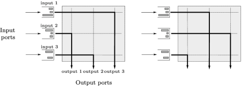
Figure 1: An input-queued switch, and two example matching of inputs to outputs.

The switch operates in discrete time. In each time slot, the switch fabric can transmit a number of packets from input ports to output ports, subject to the two constraints that each input can transmit at most one packet and that each output can receive at most one packet. In other words, at each time slot the switch can choose a matching from inputs to outputs. The schedule ${\bolds{\pi}}\in\mathbb{R}_{+}^{3\times 3}$ is given by $\pi_{i,j}=1$ if input port $i$ is matched to output port $j$ in a given time slot, and $\pi_{i,j}=0$ otherwise. Clearly ${\bolds{\pi}}$ is a permutation matrix, and the set $\mathcal{S}$ of allowed schedules is the set of $3\times 3$ permutation matrices.

Figure 1 shows two possible matchings. In the left-hand figure, the matching allows a packet to be transmitted from input port 3 to output port 2, but since $Q_{3,2}$ is empty, no packet is actually transmitted.

3 Related work.

Keslassy and McKeown KM found from extensive simulations of an input-queued switch that the average queueing delay is different under MW-$\alpha$ policies for different values of $\alpha>0$. They conjecture:

Conjecture 3.1.

For an input-queued switch running the MW-$\alpha$ policy, the average queueing delay decreases as $\alpha$ decreases.

Though our work is motivated by the desire to establish Conjecture 3.1, we have not been able to prove it. But whereas the two main analytic approaches that have been employed in the literature yield results for the input-queued switch that are insensitive to $\alpha$, our result about multiplicative state space collapse is sensitive, as shown in Section 8. We speculate that our result might eventually form part of a proof of the conjecture.

The two main analytic approaches that have been employed in the literature are stability analysis and heavy traffic analysis. In stability analysis, one calculates the set of arrival rates for which a policy is stable (in the sense of tassiula1 , MAW , daibala , KM , dev , andrewsetal ). All the prior work in this context leads to the conclusion that MW-$\alpha$ has the optimal stability region, regardless of $\alpha$.

In heavy traffic analysis, one looks at queue size behavior under a diffusion (or heavy traffic) scaling. This regime was first described by Kingman kingmanht ; since then a substantial body of theory has developed, and modern treatments can be found in mike2 , bramson , williams , whittspl . Stolyar has studied MW-$\alpha$ for a generalized switch model in the diffusion scaling, and obtained a complete characterization of the diffusion approximation for the queue size process, under a condition known as “complete resource pooling.” This condition effectively requires that a clever scheduling policy be able to balance work between all the heavily loaded queues. Stolyar stolyar showed in a remarkable paper that the limiting queue size lives in a one-dimensional state space. Operationally, this means that all one needs to keep track of is the one-dimensional total amount of work in the system (called the workload), and at any point in time one can assume that the individual queues have all been balanced. Dai and Lin LD05 , LD08 have established that similar result holds in the more general setting of a stochastic processing network.

Under the complete resource pooling condition, the results in stolyar , LD05 , LD08 imply that the performance of MW-$\alpha$ in an input-queued switch is always optimal (in the diffusion scaling) regardless of the value of $\alpha>0$. Therefore these results do not help in addressing Conjecture 3.1. This is our motivation for studying switched networks in the absence of complete resource pooling. Technically, the lifting map for a critically-loaded input-queued switch is degenerate and insensitive to $\alpha$ under complete resource pooling, but it is sensitive to $\alpha$ otherwise.

We prove multiplicative state space collapse, following the method of Bramson bramson . The complement of Bramson’s work is by Williams williams , and consists of proving a diffusion approximation, using an appropriate invariance principle along with the multiplicative state space collapse. We do not carry out this complementary aspect. Stolyar stolyar and Dai and Lin LD05 , LD08 have proved the diffusion approximation under the complete resource pooling condition, and Kang and Williams KW have made progress toward it in the case without complete resource pooling, for an input-queued switch under the MW-$1$ policy.

Whereas in heavy traffic models of other systems mike2 , bramson , williams , stolyar the lifting map from workloads to queue sizes is linear, we find instead that it is nonlinear—in fact it can be expressed as the solution to an optimization problem. The objective function of the problem is a natural generalization of the Lyapunov function introduced by Tassiulas and Ephremides tassiula1 for proving stability of the MW-$1$ policy; the constraints of the problem are closely linked to the canonical representation of workload identified by Harrison harrisoncanonical . The objective function for MW-$\alpha$ depends on $\alpha$, and this hints that the performance measures might also depend on $\alpha$.

Finally, we take note of two related results. First, in shahwischikinfocom we have reported some results about a critically loaded input-queued switch without a complete resource pooling condition. Second, a sequence of works by Kelly and Williams KW04 and Kang et al. kellywilliamsssc has resulted in a diffusion approximation for a bandwidth sharing network model operating under proportionally fair rate allocation, assuming a technical “local traffic” condition, but without assuming complete resource pooling. They show that the resulting diffusion approximation model has a product form stationary distribution.

4 The fluid approximation.

This section introduces the fluid model and establishes it as an approximation to a fluid-scaled descriptor of the switched network. Intuitively, the fluid model describes the dynamics of the system at the “rate” level rather than at finer granularity. The reader is referred to a recent monography by Bramson Bramson08 and lecture notes by Dai dailec for a detailed account of fluid approximation for multiclass queueing networks. In Section 4.1 we specify the fluid model, in Section 4.2 we state the main result and in Section 4.3 we prove it.

4.1 Definition of fluid model.

Let time be measured by $t\in[0,T]$ for some fixed $T>0$. Let $\mathbf{q}$, $\mathbf{a}$ and $\mathbf{y}$ all be continuous functions mapping $[0,T]$ into $\mathbb{R}_{+}^{N}$, and let $s=(s_{\bolds{\pi}})_{{\bolds{\pi}}\in\mathcal{S}}$ be a collection of continuous functions mapping $[0,T]$ into $\mathbb{R}_{+}$. Let $x(\cdot)=(\mathbf{q}(\cdot),\mathbf{a}(\cdot),\mathbf{y}(\cdot),s(\cdot))$. This lies in $C^{I}(T)$ where $I=3N+|\mathcal{S}|$. The definition below requires these functions to be absolutely continuous; such functions are differentiable almost everywhere, and the time instants where they are differentiable are called “regular times.” Any equations we write involving derivatives are taken to apply only at regular times.

Definition 4.1 ((Fluid model solution for single-hop network)).

Let $f\dvtx\allowbreak\mathbb{R}_{+}\to\mathbb{R}_{+}$ satisfy Assumption 2.1. Say that $x(\cdot)$ is a fluid model solution for a single-hop switched network with arrival rate $\bolds{\lambda}\in\mathbb{R}_{+}^{N}$ operating under the MW-$f$ policy if it satisfies equations (13)–(4.1) below. Write $\operatorname{FMS}$ for the set of all such $x\in C^{I}(T)$. Additionally, define

$$\operatorname{FMS}_{K} = \{x\in\operatorname{FMS}\dvtx|\mathbf{q}(0)|\leq K\},$$

$$\operatorname{FMS}(\mathbf{q}_{0}) = \{x\in\operatorname{FMS}\dvtx\mathbf{q}(0)=\mathbf{q}_{0}\}.$$

The equations are:

$$\mathbf{q}(t) = \mathbf{q}(0)+\mathbf{a}(t)-\sum_{{\bolds{\pi}}}s_{\bolds{\pi}}(t){\bolds{\pi}}+\mathbf{y}(t);$$ (13)

$$\mathbf{a}(t) = \bolds{\lambda}t;$$ (14)

$$\sum_{{\bolds{\pi}}\in\mathcal{S}}s_{{\bolds{\pi}}}(t) = t;$$ (15)

$$\mathbf{y}(t) \leq \sum_{{\bolds{\pi}}\in\mathcal{S}}s_{{\bolds{\pi}}}(t){\bolds{\pi}};$$ (16)

$$\mbox{each $s_{\bolds{\pi}}(\cdot)$ and $y_{n}(\cdot)$ is increasing (not necessarily strictly increasing)};$$

$$\mbox{all the components of $x(\cdot)$ are absolutely continuous};$$

$$\mbox{for regular times $t$, all }n\qquad\dot{y}_{n}(t)=0\qquad\mbox{if $q_{n}(t)>0$};$$

$$\mbox{for regular times $t$, all }{\bolds{\pi}}\in\mathcal{S}$$

$$\qquad\dot{s}_{\bolds{\pi}}(t)=0\qquad\mbox{if }{\bolds{\pi}}\cdot f(\mathbf{q}(t))<\max_{{\bolds{\rho}}\in\mathcal{S}}{\bolds{\rho}}\cdot f(\mathbf{q}(t)).$$

Here, $\mathbf{q}(t)$ represents the vector of queue sizes at time $t$, $\mathbf{a}(t)$ represents the cumulative arrivals up to time $t$, $\mathbf{y}(t)$ represents the cumulative idleness up to time $t$ and $s_{\bolds{\pi}}(t)$ represents the total amount of time spent on schedule ${\bolds{\pi}}$ up to time $t$. The equation in (13) is the continuous analog of (4) combined with (5), and the inequality is the analog of the single-hop version of (7). Equation (14) represents an assumption about the arrival process, related to (11). Equation (15) says that the scheduling policy must choose some schedule at every timestep. Both (16) and (4.1) derive from the definition of idling, (3). Equation (4.1) is the continuous analog of (9).

Definition 4.2 ((Fluid model solution for multi-hop network)).

Let $f\dvtx\allowbreak\mathbb{R}_{+}\to\mathbb{R}_{+}$ satisfy Assumption 2.2, and let $\mathcal{S}$ satisfy Assumption 2.3. Say that $x(\cdot)$ is a fluid model solution for a multi-hop switched network operating under the MW-$f$ policy if it satisfies equations (14)–(4.1), and additionally (21) and (4.2) below. Let $\operatorname{FMSm}$ be the set of all such $x\in C^{I}(T)$. Also, let $\operatorname{FMSm}_{K}$ and $\operatorname{FMSm}(\mathbf{q}_{0})$ be defined analogously to the single-hop case. The extra equations are

$$\mathbf{q}(t)=\mathbf{q}(0)+\mathbf{a}(t)-(I-R^{\mathsf{T}})\biggl{(}\sum_{{\bolds{\pi}}}s_{\bolds{\pi}}(t){\bolds{\pi}}-\mathbf{y}(t)\biggr{)}$$ (21)

and

for all regular times $$t {\bolds{\pi}}\in\mathcal{S}$$, all

(22)

$$\qquad\dot{s}_{\bolds{\pi}}(t)=0\qquad\mbox{if }{\bolds{\pi}}\cdot(I-R)f(\mathbf{q}(t))<\max_{{\bolds{\rho}}\in\mathcal{S}}{\bolds{\rho}}\cdot(I-R)f(\mathbf{q}(t)).$$

When we refer to “fluid model solutions for any scheduling policy,” we mean processes $x(\cdot)\in C^{I}(T)$ satisfying (13) to (4.1) in the single-hop case, or satisfying (14) to (4.1) plus (21) in the multi-hop case.

4.2 Main fluid model result.

The development in this section follows the general pattern of Bramson bramson . There is, however, a difference in presentation that is worth noting. The main result of this section, Theorem 4.3, is a general purpose sample path-wise result: it does not make any probabilistic claim nor does it depend on any probabilistic assumptions. It can be applied to a switched network with stochastic arrivals in two ways: to obtain a result about fluid approximations (Corollary 4.4), and to obtain a result about multiplicative state space collapse (Section 7).

We start by defining the fluid scaling. Consider a switched network of the type described in Section 2.1 running a scheduling policy of the type described in Section 2.2. Write $X(\tau)=(\mathbf{Q}(\tau),\mathbf{A}(\tau),\mathbf{Y}(\tau),S(\tau))$, $\tau\in\mathbb{Z}_{+}$, to denote its sample path. Given a scaling parameter $z\geq 1$, define the fluid-scaled sample path $\tilde{x}(t)=(\tilde{\mathbf{q}}(t),\tilde{\mathbf{a}}(t),\tilde{\mathbf{y}}(t),\tilde{s}(t))$ for $t\in\mathbb{R}_{+}$ by

$$\tilde{\mathbf{q}}(t) = \mathbf{Q}(zt)/z,\qquad\tilde{\mathbf{a}}(t)=\mathbf{A}(zt)/z,$$

$$\tilde{\mathbf{y}}(t) = \mathbf{Y}(zt)/z,\qquad\tilde{s}_{\bolds{\pi}}(t)=S_{\bolds{\pi}}(zt)/z$$

after extending the domain of $X(\cdot)$ to $\mathbb{R}_{+}$ by linear interpolation in each interval $(\tau,\tau+1)$. In this section we are interested in the evolution of $\tilde{x}(t)$ over $t\in[0,T]$ for some fixed $T>0$, therefore we take $\tilde{x}$ to lie in $C^{I}(T)$ with $I=3{N}+|\mathcal{S}|$.

The following theorem concerns uniform convergence of a set of fluid-scaled sample paths. Every fluid-scaled sample path is assumed to relate to some (unscaled) switched network, and all the switched networks are assumed to have the same network data, that is, the same number of queues $N$, the same set of allowed schedules $\mathcal{S}$, the same routing matrix $R$, and the same scheduling policy.

The convergence is indexed by a parameter $j$ lying in some totally ordered countable set. For Corollary 4.4 we will use $j\in\mathbb{N}$, and for Section 7 we will use a subset of $\mathbb{N}\times\mathbb{N}$ as the index set. We are purposefully using the symbol $j$ here as an index, rather than the $r$ used elsewhere, to remind the reader that the index set is interpreted differently in different results.

Theorem 4.3.

Let $\mathcal{X}$ be the set of all possible sample paths for single-hop switched networks with the network data specified above, running the MW-$f$ scheduling policy, where $f$ satisfies Assumption 2.1. Fix $K>0$ and $\bolds{\lambda}\in\mathbb{R}_{+}^{N}$. Let there be sequences $\varepsilon_{j}\in\mathbb{R}_{+}$ and $\bolds{\lambda}^{j}\in\mathbb{R}_{+}^{N}$, indexed by $j$ in some totally ordered countable set, such that

$$\varepsilon_{j}\to 0\quad\mbox{and}\quad\bolds{\lambda}^{j}\to\bolds{\lambda},\qquad\mbox{as $j\to\infty$}.$$ (23)

Consider a sequence of subsets $G_{j}\subset C^{I}(T)\times[1,\infty)$ which satisfy the following: for every $(\tilde{x},z)\in G_{j}$ there is some unscaled sample path $X\in\mathcal{X}$ such that $\tilde{x}$ is the fluid-scaled version of $X$ with scaling parameter $z$ (here $z$ is permitted to be a function of $X$); and furthermore

$$\inf\{z\dvtx(\tilde{x},z)\in G_{j}\} \to \infty\qquad\mbox{as $j\to\infty$,}$$ (24)

$$\sup_{(\tilde{x},z)\in G_{j}}\sup_{t\in[0,T]}|\tilde{\mathbf{a}}(t)-\bolds{\lambda}^{j}t| \leq \varepsilon_{j}\qquad\mbox{for all $j$}$$ (25)

and

$$\sup_{(\tilde{x},z)\in G_{j}}|\tilde{\mathbf{q}}(0)|\leq K\qquad\mbox{for all $j$.}$$ (26)

Then

$$\sup_{(\tilde{x},z)\in G_{j}}d(\tilde{x},\operatorname{FMS}_{K})\to 0\qquad\mbox{as $j\to\infty$}.$$ (27)

Furthermore, fix $\mathbf{q}_{0}\in\mathbb{R}_{+}^{N}$ and a sequence $\varepsilon^{\prime}_{j}\to 0$, and assume that the sets $G_{j}$ also satisfy

$$\sup_{(\tilde{x},z)\in G_{j}}|\tilde{\mathbf{q}}(0)-\mathbf{q}_{0}|\leq\varepsilon^{\prime}_{j}\qquad\mbox{for all $j$}.$$ (28)

Then

$$\sup_{(\tilde{x},z)\in G_{j}}d(\tilde{x},\operatorname{FMS}(\mathbf{q}_{0}))\to 0\qquad\mbox{as $j\to\infty$}.$$ (29)

Equivalent results to (27) and (29) apply to multi-hop switched networks, with references to $\operatorname{FMS}$ replaced by $\operatorname{FMSm}$ and the set $\mathcal{X}$ modified to refer to multi-hop networks running the MW-$f$ scheduling policy where $f$ satisfies Assumption 2.2 and $\mathcal{S}$ satisfies Assumption 2.3.

The above theorem as stated applies to the MW-$f$ scheduling policy, but it is clear from the proof that a corresponding limit result holds, relating sample paths of any scheduling policy to fluid models defined by equations (13)–(4.1).

The following corollary is a straightforward application of Theorem 4.3. It specializes the theorem to the case of a single random system $X$, and the sequence of fluid-scaled versions indexed by $r\in\mathbb{N}$ where the $r$th version uses scaling parameter $r$. The arrival process is assumed to satisfy certain stochastic assumptions. This corollary is useful when studying the behavior of a single switched network with random arrivals, over long timescales.

Corollary 4.4.

Consider a single-hop switched network as described in Section 2.1, running the MW-$f$ policy as described in Section 2.2 where $f$ satisfies Assumption 2.1. Let the arrival process $\mathbf{A}(\cdot)$ satisfy Assumption 2.4, and let the initial queue size $\mathbf{Q}(0)\in\mathbb{R}_{+}^{N}$ be random. For $r\in\mathbb{N}$, let

$$\tilde{\mathbf{q}}^{r}(t) = \mathbf{Q}(rt)/r,\qquad\tilde{\mathbf{a}}^{r}(t)=\mathbf{A}(rt)/r,$$

$$\tilde{\mathbf{y}}^{r}(t) = \mathbf{Y}(rt)/r,\qquad\tilde{s}_{\bolds{\pi}}^{r}(t)=S_{\bolds{\pi}}(rt)/r,$$

and let $\tilde{x}^{r}(t)=(\tilde{\mathbf{q}}^{r}(t),\tilde{\mathbf{a}}^{r}(t),\tilde{\mathbf{y}}^{r}(t),\tilde{s}^{r}(t))$, for $t\in[0,T]$ where $T>0$ is some fixed time horizon. Then for any $\delta>0$

$$\mathbb{P}\bigl{(}d(\tilde{x}^{r}(\cdot),\operatorname{FMS}(\mathbf{0}))<\delta\bigr{)}\to 1\qquad\mbox{as $r\to\infty$}.$$

The same conclusion holds for a multi-hop switched network running the MW-$f$ back-pressure policy where $f$ satisfies Assumption 2.2 and $\mathcal{S}$ satisfies Assumption 2.3, with $\operatorname{FMS}$ replaced by $\operatorname{FMSm}$.

First define the event $E_{r}$ by

$$E_{r}=\biggl{\{}\sup_{\tau\leq r}\frac{1}{r}|\mathbf{A}(\tau)-\bolds{\lambda}\tau|<\delta_{r}\quad\mbox{and}\quad|\mathbf{Q}(0)|\leq\sqrt{r}\biggr{\}},$$

where $\bolds{\lambda}$ and $\delta_{r}$ are as in Assumption 2.4. By this we mean that $E_{r}$ is a subset of the probability sample space, and we write $X(\cdot)(\omega)$ etc. for $\omega\in E_{r}$ to emphasize the dependence on $E_{r}$.

We will apply Theorem 4.3 with index set $j\equiv r\in\mathbb{N}$ to the sequence of sets

$$G_{j}\equiv G_{r}=\{(\tilde{x}^{r}(\cdot)(\omega),r)\dvtx\omega\in E_{r}\}.$$

In order to apply the theorem we will pick constants as follows. Let $K=1$, let $\bolds{\lambda}$ be as in Assumption 2.4, $\bolds{\lambda}^{j}=\bolds{\lambda}$ for all $j$, $\varepsilon_{j}\equiv\varepsilon_{r}=T\delta_{r}$ where $\delta_{r}$ is as in Assumption 2.4, $\mathbf{q}_{0}=\mathbf{0}$ and $\varepsilon^{\prime}_{r}=1/\sqrt{r}$. We now need to verify the conditions of Theorem 4.3. Equation (23) holds by the choice of $\bolds{\lambda}^{j}$ and by Assumption 2.4. Equation (24) holds automatically by choice of $G_{j}$. To see that (25) holds, rewrite event $E_{r}$ in terms of the fluid scaled arrival process $\tilde{\mathbf{a}}^{r}$ to see

$$\sup_{t\in[0,T]}|\tilde{\mathbf{a}}^{r}(t)(\omega)-\bolds{\lambda}t|<T\delta_{r}\qquad\mbox{for all $r$ and $\omega\in E_{r}$},$$

which implies (25); likewise for (26) and (28). We conclude that (29) holds. It may be rewritten in terms of $E_{r}$ as

$$\sup_{\omega\in E_{r}}d(\tilde{x}^{r}(\cdot)(\omega),\operatorname{FMS}(\mathbf{0}))\to 0\qquad\mbox{as $r\to\infty$.}$$ (30)

We next argue that $\mathbb{P}(E_{r})\to 1$ as $r\to\infty$. The event $E_{r}$ is the intersection of two events, one concerning arrivals and the other concerning initial queue size. The probability of the former $\to 1$ as $r\to\infty$ by Assumption 2.4. For the latter, $\mathbb{P}(|\mathbf{Q}(0)|\leq\sqrt{r})\to 1$ as $r\to\infty$ since $\mathbf{Q}(0)$ is assumed not to be infinite. Therefore $\mathbb{P}(E_{r})\to 1$. Combining this with (30) gives the desired result for single-hop networks. The multi-hop version follows similarly.

4.3 Proof of Theorem 4.3.

We shall present the proof of Theorem 4.3 for a single-hop network in detail followed by main ideas required to extend it to multi-hop networks.

4.3.1 Cluster points.

Here we are interested in convergence in $C^{I}(T)$, where $I=3N+|\mathcal{S}|$ and $T>0$ is fixed, equipped with the norm $\|\cdot\|$. The appropriate concept for proving convergence is cluster points. Consider any metric space $E$ with metric $d$ and a sequence $(E_{1},E_{2},\ldots)$ of subsets of $E$. Say that $x\in E$ is a cluster point of the sequence if $\liminf_{j\to\infty}d(x,E_{j})=0$ where $d(x,E_{j})=\inf\{d(x,y)\dvtx y\in E_{j}\}$.

Proposition 4.5 ([Cluster points in $C^{I}(T)$]).

Given $K>0$, $A>0$ and a sequence $B_{j}\to 0$, let

$$K_{j}=\{x\in C^{I}(T)\dvtx|x(0)|\leq K\mbox{ and }\operatorname{mc}_{\delta}(x)\leq A\delta+B_{j}\mbox{ for all $\delta>0$}\},$$

and consider a sequence $(E_{1},E_{2},\ldots)$ of subsets of $C^{I}(T)$ for which $E_{j}\subset K_{j}$. Then $\sup_{y\in E_{j}}d(y,\mathrm{CP})\to 0$ as $j\to\infty$, where $\mathrm{CP}$ is the set of cluster points of $(E_{1},E_{2},\ldots)$.

4.3.2 Proof of Theorem 4.3.

Let $E_{j}=\{\tilde{x}\dvtx(\tilde{x},z)\in G_{j}\}$. Lemma 4.6 below shows that $E_{j}\subset K_{j}$, with $K_{j}$ as defined in Proposition 4.5 for appropriate constants $K$, $A$ and $B_{j}$. By applying that proposition,

$$\sup_{\tilde{x}\in E_{j}}d(\tilde{x},\mathrm{CP})\to 0\qquad\mbox{as $j\to\infty$},$$

where $\mathrm{CP}$ is the set of cluster points of the $E_{j}$ sequence. Lemma 4.7 below shows that all cluster points of the $E_{j}$ sequence satisfy the fluid model equations. Every cluster point $x$ must also satisfy $|\mathbf{q}(0)|\leq K$, by (26). Therefore

$$\sup_{\tilde{x}\in E_{j}}d(\tilde{x},\operatorname{FMS}_{K})\to 0\qquad\mbox{as $j\to\infty$}.$$

If in addition (28) holds, then every cluster point $x$ must also satisfy $\mathbf{q}(0)=\mathbf{q}_{0}$. Therefore

$$\sup_{\tilde{x}\in E_{j}}d(\tilde{x},\operatorname{FMS}(\mathbf{q}_{0}))\to 0\qquad\mbox{as $j\to\infty$}.$$

Lemma 4.6 ((Tightness of fluid scaling)).

Let $K$ and $G_{j}$ be as in Theorem 4.3. Then there exist a constant $A>0$ and a sequence $B_{j}\to 0$ such that for every $(\tilde{x},z)\in G_{j}$, $|\tilde{x}(0)|\leq K$ and

$$|\tilde{x}(u)-\tilde{x}(t)|\leq A|u-t|+B_{j}\qquad\mbox{for all $0\leq t,u\leq T$.}$$

Consider $(\tilde{x},z)\in G_{j}$, where $\tilde{x}=(\tilde{\mathbf{q}},\tilde{\mathbf{a}},\tilde{\mathbf{y}},\tilde{s})$. As per the definitions in Section 2.1, the only nonzero component of $\tilde{x}(0)$ is $\tilde{\mathbf{q}}(0)$ and $|\tilde{\mathbf{q}}(0)|\leq K$ by choice of $G_{j}$, hence $|\tilde{x}(0)|\leq K$. For the second inequality, without loss of generality pick any $0\leq t<u\leq T$, and let us now look at each component of $|\tilde{x}(u)-\tilde{x}(t)|$ in turn.

For arrivals, let $\lambda^{\max}=\sup_{j}|\bolds{\lambda}^{j}|$; this is finite by the assumption that $\bolds{\lambda}^{j}\to\bolds{\lambda}$ in Theorem 4.3. Then for $(\tilde{x},z)\in G_{j}$,

$$|\tilde{\mathbf{a}}(u)-\tilde{\mathbf{a}}(t)| \leq |\tilde{\mathbf{a}}(u)-\bolds{\lambda}^{j}u|+|\bolds{\lambda}^{j}(u-t)|+|\tilde{\mathbf{a}}(t)-\bolds{\lambda}^{j}t|$$

$$\leq 2\varepsilon_{j}+|\bolds{\lambda}^{j}|(u-t)\qquad\mbox{by (\ref{eq:fluid.arr})}$$

$$\leq 2\varepsilon_{j}+\lambda^{\max}(u-t).$$

For idling, let $S^{\max}=\max_{{\bolds{\pi}}\in\mathcal{S}}\max_{n}\pi_{n}$. This is the maximum amount of service that can be offered to any queue per unit time, and it must be finite since $|\mathcal{S}|$ is finite. Then, based on (3),

$$|\tilde{y}_{n}(u)-\tilde{y}_{n}(t)| \leq (u-t)S^{\max}+2S^{\max}/z$$

$$\leq (u-t)S^{\max}+2S^{\max}/z_{j}^{\min},$$

where $z_{j}^{\min}=\inf\{z\dvtx(\tilde{x},z)\in G_{j}\}$. For service, let $S_{\bolds{\pi}}(\cdot)$ be the unscaled process that corresponds to $\tilde{s}_{\bolds{\pi}}(\cdot)$; since $S_{\bolds{\pi}}(\cdot)$ is increasing and since a schedule must be chosen not more than once every time slot,

$$|\tilde{s}_{\bolds{\pi}}(u)-\tilde{s}_{\bolds{\pi}}(t)|\leq\frac{1}{z}\bigl{(}S_{\bolds{\pi}}(\lceil zu\rceil)-S_{\bolds{\pi}}(\lfloor zt\rfloor)\bigr{)}\leq(u-t)+2/z\leq(u-t)+2/z_{j}^{\min}.$$

For queue size, note that (4) carries through to the fluid model scaling, that is,

$$\tilde{\mathbf{q}}(t)=\tilde{\mathbf{q}}(0)+\tilde{\mathbf{a}}(t)-\sum_{\bolds{\pi}}\tilde{s}_{\bolds{\pi}}(t){\bolds{\pi}}+\tilde{\mathbf{y}}(t),$$

thus

$$|\tilde{q}_{n}(u)-\tilde{q}_{n}(t)|$$

$$\qquad\leq|\tilde{a}_{n}(u)-\tilde{a}_{n}(t)|+\sum_{\bolds{\pi}}\pi_{n}|\tilde{s}_{\bolds{\pi}}(u)-\tilde{s}_{\bolds{\pi}}(t)|+|\tilde{y}_{n}(u)-\tilde{y}_{n}(t)|$$

$$\qquad\leq(u-t)(\lambda^{\max}+|\mathcal{S}|S^{\max}+S^{\max})+(2|\mathcal{S}|S^{\max}+2S^{\max})/z_{j}^{\min}+2\varepsilon_{j}.$$

Putting all these together,

$$|\tilde{x}(u)-\tilde{x}(t)|\leq A(u-t)+B_{j},$$ (31)

where the constants are

$$A=(N+1)\lambda^{\max}+2NS^{\max}+|\mathcal{S}|+N|\mathcal{S}|S^{\max}$$

and

$$B_{j}=(4NS^{\max}+2|\mathcal{S}|+2N|\mathcal{S}|S^{\max})\frac{1}{z_{j}^{\min}}+(2+2N)\varepsilon_{j}.$$

By the assumptions of Theorem 4.3, $\varepsilon_{j}\to 0$ and $z_{j}^{\min}\to\infty$ as $j\to\infty$, thus $B_{j}\to 0$ as required.

Lemma 4.7 ((Dynamics at cluster points)).

Make the same assumptions as Theorem 4.3, and let $E_{j}=\{\tilde{x}\dvtx(\tilde{x},z)\in G_{j}\}$. Then $x\in\operatorname{FMS}_{K}$ if $x$ is a cluster point of the $E_{j}$ sequence.

From Lemma 4.6 and Proposition 4.5, it follows that$\limsup_{\tilde{x}\in E_{j}}d(\tilde{x}$, $\mathrm{CP})\to 0$ as $j\to\infty$ where $\mathrm{CP}$ is the set of cluster points of the sequence $E_{j}$. Let $x$ be one such cluster point. That is, there exists a subsequence $j_{k}$ and a collection $\tilde{x}^{j_{k}}\in E_{j_{k}}$ such that $\tilde{x}^{j_{k}}\to x$. It easily follows that $|x(0)|\leq K$ since $|\tilde{x}^{j_{k}}(0)|\leq K$ for all $\tilde{x}^{j_{k}}\in E_{j_{k}}$ as argued in Lemma 4.6. Using this, we wish to establish that $x$ satisfies all the fluid model equations to conclude $x\in\operatorname{FMS}_{K}$. For convenience, we shall omit the subscript $k$ in the rest of the proof; that is, we shall use $j$ in place of $j_{k}$ and $j\to\infty$.

Proof of (13), (15), (4.1). The discrete (unscaled) system satisfies these properties; therefore the scaled systems $\tilde{x}^{j}$ do too. Taking the limit yields the fluid equations.

Proof of (16). In (3), $d\mathbf{B}(\tau)$ and $\mathbf{Q}(\tau)$ are both nonnegative (component-wise), hence $d\mathbf{Y}(\tau)\leq d\mathbf{B}(\tau)$ for all $\tau$. Summing up over $\tau$, we see the discrete (unscaled) system satisfies the equivalent of (16), so as above we obtain the fluid equation.

Proof of (14). Observe that

$$\sup_{t\in[0,T]}|\mathbf{a}(t)-\bolds{\lambda}t|\leq\sup_{t\in[0,T]}|\mathbf{a}(t)-\tilde{\mathbf{a}}^{j}(t)|+\sup_{t\in[0,T]}|\tilde{\mathbf{a}}^{j}(t)-\bolds{\lambda}^{j}t|+T|\bolds{\lambda}^{j}-\bolds{\lambda}|.$$

Each term converges to 0 as $j\to\infty$: the first because $\tilde{x}^{j}\to x$, the second because $\tilde{x}^{j}\in E_{j}$ so the deviation in $\tilde{\mathbf{a}}^{j}$ is bounded by $\varepsilon_{j}$ and $\varepsilon_{j}\to 0$ and the third because $\bolds{\lambda}^{j}\to\bolds{\lambda}$. Since the left-hand side does not depend on $j$, it must be that $\mathbf{a}(t)=\bolds{\lambda}t$.

Proof of (4.1). In Lemma 4.6 we found constants $A$ and $B_{j}$ such that for all $\tilde{x}\in E_{j}$

$$|\tilde{x}(u)-\tilde{x}(t)|\leq A|u-t|+B_{j}$$

with $B_{j}\to 0$ as $j\to\infty$. Taking the limit of $|\tilde{x}^{j}(u)-\tilde{x}^{j}(t)|$ as $j\to\infty$, we find that $|x(u)-x(t)|\leq A|u-t|$; that is, $x$ is (globally) Lipschitz continuous (of order $1$ with respect to the appropriate metric as defined earlier). This immediately implies that $x$ is absolutely continuous.

Proof of (4.1). Since $x=(\mathbf{q},\mathbf{a},\mathbf{y},s)$ is absolutely continuous, each component is too, which means that $y_{n}$ is differentiable for almost all $t$. Pick some such $t$, and suppose that $q_{n}(t)>0$. Consider some small interval $I=[t,t+\delta]$ about $t$. Since $q_{n}$ is continuous, we can choose $\delta$ sufficiently small that $\inf_{s\in I}q_{n}(s)>0$. Since $\|\tilde{\mathbf{q}}^{j}-\mathbf{q}\|\to 0$, we can find $c>0$ such that $\inf_{s\in I}\tilde{q}^{j}_{n}(s)>c$ for all $j$ sufficiently large. Since $\tilde{x}^{j}\in E_{j}$, there exists a corresponding unscaled version of the system, say $X^{j}$, and scaling parameter, say $z_{j}$, so that $\tilde{x}^{j}(\cdot)=X^{j}(z_{j}\cdot)/z_{j}$. Therefore, it must be that the corresponding unscaled queue satisfies $\inf_{s\in I}Q^{j}_{n}(z_{j}s)>z_{j}c$. That is, the queue size in the entire interval never vanishes to $0$ and hence idling in the entire interval is not possible. Therefore after rescaling we find $\tilde{y}^{j}_{n}(t+\delta/2)=\tilde{y}^{j}_{n}(t)$. (The switch from $\delta$ to $\delta/2$ sidesteps any discretization problems.) Therefore the same holds for $y_{n}$ in the limit. We assumed $y_{n}$ to be differentiable at $t$; the derivative must be $0$.

Proof of (4.1). Pick a $t$ at which $s_{\bolds{\pi}}$ is differentiable, and suppose that ${\bolds{\pi}}\cdot f(\mathbf{q}(t))<\max_{\bolds{\rho}}{\bolds{\rho}}\cdot f(\mathbf{q}(t))$. As above, pick some small interval $I=[t,t+\delta]$ and $j$ sufficiently large that

$${\bolds{\pi}}\cdot f(\tilde{\mathbf{q}}^{j}(s))<\max_{{\bolds{\rho}}\in\mathcal{S}}{\bolds{\rho}}\cdot f(\tilde{\mathbf{q}}^{j}(s))\qquad\mbox{for $s\in I$}.$$

Writing this in terms of the unscaled system and applying Assumption 2.1,

$${\bolds{\pi}}\cdot f(\mathbf{Q}^{j}(z_{j}s))<\max_{{\bolds{\rho}}\in\mathcal{S}}{\bolds{\rho}}\cdot f(\mathbf{Q}^{j}(z_{j}s))\qquad\mbox{for $s\in I$}.$$

The MW-$f$ policy ensures by (9) that ${\bolds{\pi}}$ will not be chosen throughout this entire interval, so after rescaling we find $\tilde{s}^{j}_{\bolds{\pi}}(t+\delta/2)-\tilde{s}^{j}_{\bolds{\pi}}(t)=0$, and taking the limit gives $s_{\bolds{\pi}}(t+\delta/2)=s_{\bolds{\pi}}(t)$. Since $s_{\bolds{\pi}}$ is assumed to be differentiable at $t$; the derivative must be $0$.

4.3.3 Proof of Theorem 4.3 for multi-hop networks.

The proof of Theorem 4.3 for single-hop network applies verbatim, except that the two lemmas need to be replaced.

Lemma 4.6 (Tightness of fluid scaling) $$\longrightarrow$$ Lemma 4.8.

Lemma 4.7 (Dynamics at cluster points) $$\longrightarrow$$ Lemma 4.9.

Lemma 4.8 ((Tightness of fluid scaling)).

Make the same assumptions as Theorem 4.3, multi-hop case, and use the same definition of $G_{j}$. Then there exist a constant $A>0$ and a sequence $B_{j}\to 0$ such that for every $(\tilde{x},z)\in G_{j}$, $|\tilde{x}(0)|\leq K$ and

$$|\tilde{x}(u)-\tilde{x}(t)|\leq A|u-t|+B_{j}\qquad\mbox{for all $0\leq t,u\leq T$.}$$

Consider $(\tilde{x},z)\in G_{j}$, $\tilde{x}=(\tilde{\mathbf{q}},\tilde{\mathbf{a}},\tilde{\mathbf{y}},\tilde{s})$. The bound $|\tilde{x}(0)|\leq K$ follows from an argument similar to that in the single-hop case. The bounds on the arrival process, the idleness and service allocation are as in the single-hop case: for any $0\leq t<u\leq T$,

$$|\tilde{\mathbf{a}}(u)-\tilde{\mathbf{a}}(t)| \leq (u-t)\lambda^{\max}+2\varepsilon_{j},$$

$$|\tilde{y}_{n}(u)-\tilde{y}_{n}(t)| \leq (u-t)S^{\max}+2S^{\max}/z_{j}^{\min},$$

$$|\tilde{s}_{\bolds{\pi}}(t)-\tilde{s}_{\bolds{\pi}}(s)| \leq (u-t)+2/z_{j}^{\min},$$

where $z_{j}^{\min}=\inf\{z\dvtx(\tilde{x},z)\in G_{j}\}$. The bound on queue size is a little different. Note that (6) carries through to the fluid-scaling, that is,

$$\tilde{\mathbf{q}}(t)=\tilde{\mathbf{q}}(0)+\tilde{\mathbf{a}}(t)-(I-R^{\mathsf{T}})\sum_{\bolds{\pi}}\tilde{s}_{\bolds{\pi}}(t){\bolds{\pi}}+\tilde{\mathbf{y}}(t),$$

thus

$$|\tilde{q}_{n}(u)-\tilde{q}_{n}(t)| \leq |\tilde{a}_{n}(u)-\tilde{a}_{n}(t)|+\sum_{\bolds{\pi}}|[(I-R^{\mathsf{T}}){\bolds{\pi}}]_{n}||\tilde{s}_{\bolds{\pi}}(u)-\tilde{s}_{\bolds{\pi}}(t)|$$

$${}+|\tilde{y}_{n}(u)-\tilde{y}_{n}(t)|$$

$$\leq (u-t)\bigl{(}\lambda^{\max}+|\mathcal{S}|(NS^{\max})S^{\max}+S^{\max}\bigr{)}$$

$${}+\bigl{(}2|\mathcal{S}|(NS^{\max})S^{\max}+2S^{\max}\bigr{)}/z_{j}^{\min}+2\varepsilon_{j}.$$

Putting all these together, for any $(\tilde{x},z)\in G_{j}$,

$$|\tilde{x}(u)-\tilde{x}(t)|\leq A(t-s)+B_{j},$$

where the constants $A$ and $B_{j}$ are

$$A = (1+N)\lambda^{\max}+2NS^{\max}+|\mathcal{S}|+|\mathcal{S}|(NS^{\max})^{2},$$

$$B_{j} = \bigl{(}4NS^{\max}+2|\mathcal{S}|+2|\mathcal{S}|(NS^{\max})^{2}\bigr{)}\frac{1}{z_{j}^{\min}}+(2N+2)\varepsilon_{j}.$$

Here $B_{j}\to 0$ as $j\to\infty$ since $\varepsilon_{j}\to 0$ by (23) and $z_{j}^{\min}\to\infty$ as $j\to\infty$ by (24).

Lemma 4.9 ((Dynamics at cluster points)).

Under the setup of Theorem 4.3 for a multihop network, let $E_{j}=\{\tilde{x}\dvtx(\tilde{x},z)\in G_{j}\}$. Then $x\in\operatorname{FMSm}_{K}$ if $x$ is a cluster point of the $E_{j}$ sequence.

Given a cluster point $x=(\mathbf{q},\mathbf{a},\mathbf{y},s)$, let there be $(\tilde{x}^{j},z_{j})\in G_{j}$ so that $\tilde{x}^{j}\to x$, as in the proof of Lemma 4.7. Now the bound $|x(0)|\leq K$ and equations (14)–(4.1) all work exactly as in the single-hop case, as does the queue size equation (21). The only equation that needs further argument is the MW-$f$ backpressure equation (4.2).

Proof of (4.2). Pick a $t$ at which $s_{\bolds{\pi}}$ is differentiable, and suppose that ${\bolds{\pi}}\cdot(I-R)f(\mathbf{q}(t))<\max_{\bolds{\rho}}{\bolds{\rho}}\cdot(I-R)f(\mathbf{q}(t))$. As in Lemma 4.7, proof of (4.1), it must be that there is some small interval $I=[z_{j}t,z_{j}t+z_{j}\delta]$ such that ${\bolds{\pi}}$ is not chosen for any $\tau\in I$, therefore $\dot{s}_{\bolds{\pi}}(t)=0$.

5 Fluid model behavior (single-hop case).

In this section we prove certain properties of fluid model solutions, which will be needed for the main result of this paper, multiplicative state space collapse. In order to state these properties, we first need some definitions. We then state a portmanteau theorem listing all the properties, and give an example to illustrate the definitions. The rest of the section is given over to proofs and supplementary lemmas.

This section deals with a single-hop switched network; in the next section we give corresponding results for multi-hop. Our reason for giving separate single-hop and multi-hop proofs, rather than just treating single-hop as a special case of multi-hop, is that our multi-hop results place additional restrictions on the set of allowed schedules (Assumption 2.3) beyond what is required for single-hop networks. This mainly affects the proof; the portmanteau theorem for multi-hop is nearly identical to that for single-hop.

Definition 5.1 ((Admissible region)).

Let $\mathcal{S}\subset\mathbb{R}_{+}^{N}$ be the set of allowed schedules. Let $\langle{\mathcal{S}}\rangle$ be the convex hull of $\mathcal{S}$,

$$\langle{\mathcal{S}}\rangle=\biggl{\{}\sum_{{\bolds{\pi}}\in\mathcal{S}}\alpha_{\bolds{\pi}}{\bolds{\pi}}\dvtx\sum_{{\bolds{\pi}}\in\mathcal{S}}\alpha_{\bolds{\pi}}=1\mbox{, and }\alpha_{\bolds{\pi}}\geq 0\mbox{ for all ${\bolds{\pi}}$}\biggr{\}}.$$

Define the admissible region $\Lambda$ to be

$$\Lambda=\{\bolds{\lambda}\in\mathbb{R}_{+}^{N}\dvtx\bolds{\lambda}\leq\bolds{\sigma}\mbox{ componentwise, for some $\bolds{\sigma}\in\langle{\mathcal{S}}\rangle$}\}.$$

Definition 5.2 ((Static planning problems and virtual resources)).

Define the optimization problem $\operatorname{PRIMAL}(\bolds{\lambda})$ for $\bolds{\lambda}\in\mathbb{R}_{+}^{N}$ to be

$$\mbox{minimize }\sum_{{\bolds{\pi}}\in\mathcal{S}}\alpha_{\bolds{\pi}}\quad\mbox{over}\quad\alpha_{\bolds{\pi}}\in\mathbb{R}_{+}\qquad\mbox{for all ${\bolds{\pi}}\in\mathcal{S}$}$$

$$\mbox{such that }\bolds{\lambda}\leq\sum_{{\bolds{\pi}}\in\mathcal{S}}\alpha_{\bolds{\pi}}{\bolds{\pi}}\mbox{ componentwise}.$$

Let $()$ be the dual to this: it is

$$\mbox{maximize }{\bolds{\xi}}\cdot\bolds{\lambda}\quad\mbox{over}\quad{\bolds{\xi}}\in\mathbb{R}_{+}^{N}\qquad\mbox{such that }\max_{{\bolds{\pi}}\in\mathcal{S}}{\bolds{\xi}}\cdot{\bolds{\pi}}\leq 1.$$

Let $E$ be the set of extreme points of the feasible region of the dual problem; the feasible region is a finite convex polytope so $E$ is finite. Define the set of virtual resources $\mathcal{S}^{*}\subset\mathbb{R}_{+}^{N}$ to be the set of maximal extreme points,

$$\mathcal{S}^{*}=\{{\bolds{\xi}}\in E\dvtx\mbox{for all }{\bolds{\zeta}}\in E,{\bolds{\xi}}\leq{\bolds{\zeta}}\Longrightarrow{\bolds{\xi}}={\bolds{\zeta}}\}.$$

Define the set of critically loaded virtual resources $\Xi(\bolds{\lambda})$ to be

$$\Xi(\bolds{\lambda})=\{{\bolds{\xi}}\in\mathcal{S}^{*}\dvtx{\bolds{\xi}}\cdot\bolds{\lambda}=1\}.$$

Both problems are clearly feasible, and the optimum is attained in each. By Slater’s condition there is strong duality, that is, $\operatorname{PRIMAL}(\bolds{\lambda})=()$. [When we write $\operatorname{PRIMAL}(\bolds{\lambda})$ or $()$ in mathematical expressions, we mean the optimum value, not the optimizer.] Clearly, $\operatorname{PRIMAL}(\bolds{\lambda})\leq 1$ if and only if $\bolds{\lambda}$ is feasible.

Laws lawsphd , lawsaap and Kelly and Laws kellylawsrespool used primal and dual problems of this general sort for describing multi-hop queueing networks with routing choice. Harrison harrisoncanonical extended the problems for stochastic processing networks.

Definition 5.3 ((Lyapunov function and lifting map)).

Let the scheduling policy be MW-$f$, where $f$ satisfies Assumption 2.1. Define the function $L\dvtx\mathbb{R}_{+}^{N}\to\mathbb{R}_{+}$ by

$$L(\mathbf{q})=F(\mathbf{q})\cdot\mathbf{1},$$

where $F(x)=\int_{0}^{x}f(y)\,dy$ for $x\in\mathbb{R}$, and $F(\mathbf{q})=[F(q_{n})]_{1\leq n\leq N}$ as per the notation in Section 1. Define the optimization problem $\operatorname{ALGD}(\mathbf{q})$ to be

$$\mbox{minimize }L(\mathbf{r})\quad\mbox{over}\quad\mathbf{r}\in\mathbb{R}_{+}^{N}$$

$$\mbox{such that }{\bolds{\xi}}\cdot\mathbf{r}\geq{\bolds{\xi}}\cdot\mathbf{q}\qquad\mbox{for all }{\bolds{\xi}}\in\Xi(\bolds{\lambda})\quad\mbox{and}$$

$$\hphantom{\mbox{such that }}r_{n}\leq q_{n}\qquad\mbox{for all $n$ such that $\lambda_{n}=0$}.$$

Note that $F$ is strictly convex and increasing, and the feasible region is convex; hence this problem has a unique optimizer. Define the lifting map $\Delta{W}\dvtx\mathbb{R}_{+}^{N}\to\mathbb{R}_{+}^{N}$ by setting $\Delta{W}(\mathbf{q})$ to be the optimizer.

Note that $\operatorname{ALGD}$ and $\Delta{W}$ both depend on $\bolds{\lambda}$ and $f$, but we will surpress this dependency when the context makes it clear which $\bolds{\lambda}$ and $f$ are meant.

The results in this section apply to any $\bolds{\lambda}\in\Lambda$. However, if $\operatorname{PRIMAL}(\bolds{\lambda})<1$, then $\Xi(\bolds{\lambda})$ is empty, so $\Delta{W}(\mathbf{q})=\mathbf{0}$ for all $\mathbf{q}$. The results are only interesting when $\operatorname{PRIMAL}(\bolds{\lambda})=1$, so we define

$$\partial\Lambda=\{\bolds{\lambda}\in\Lambda\dvtx\operatorname{PRIMAL}(\bolds{\lambda})=1\}.$$

We can now state the main result of this section.

Theorem 5.4 ((Portmanteau theorem, single-hop version)).

Let $\bolds{\lambda}\in\Lambda$. Consider a single-hop switched network running MW-$f$, where $f$ satisfies Assumption 2.1.

For any $K<\infty$, $\{\mathbf{q}\in\mathbb{R}_{+}^{N}\dvtx L(\mathbf{q})\leq K\}$ is compact. Also, for any fluid model solution with arrival rate $\bolds{\lambda}$, $L(\mathbf{q}(t))\leq L(\mathbf{q}(0))$ for all $t\geq 0$.

$\Delta{W}$ is continuous.

If $\mathbf{q}=\Delta{W}(\mathbf{q})$, then $\Delta W(\kappa\mathbf{q})=\kappa\Delta{W}(\mathbf{q})$ for all $\kappa>0$.

Say that $\mathbf{q}^{0}$ is an invariant state if all fluid model solutions $\mathbf{q}(\cdot)$ with arrival rate $\bolds{\lambda}$, starting at $\mathbf{q}(0)=\mathbf{q}^{0}$, satisfy $\mathbf{q}(t)=\mathbf{q}^{0}$ for all $t\geq 0$. Then $\mathbf{q}^{0}$ is an invariant $\mbox{state}\iff\mathbf{q}^{0}=\Delta{W}(\mathbf{q}^{0})$.

For any $\varepsilon>0$ there exists some $H_{\varepsilon}<\infty$ such that, if $\mathbf{q}(\cdot)$ is a fluid model solution with arrival rate $\bolds{\lambda}$, and $|\mathbf{q}(0)|\leq 1$, then $|\mathbf{q}(t)-\Delta{W}(\mathbf{q}(t))|<\varepsilon$ for all $t\geq H_{\varepsilon}$.

A loose interpretation of these results is that the MW-$f$ scheduling policy seeks always to reduce $L(\mathbf{q})$ [part (i)], but it is constrained from reducing it too much, because it is not permitted to reduce the workload at any of the critically loaded virtual resource (the constraints of $\operatorname{ALGD}$). However, it can choose how to allocate work between queues, subject to those constraints. It heads towards a state where it is impossible to reduce $L(\mathbf{q})$ any further [parts (iv) and (v)]. In all the examples we have looked at, the fluid model solutions reach an invariant state in finite time, that is, (v) holds also for $\varepsilon=0$, but we have not been able to prove this in general.

5.1 Example to illustrate $\Lambda$, $\partial\Lambda$, $\mathcal{S}^{*}$ and $\Xi$.

Consider a system with $N=2$ queues, $A$ and $B$. Suppose the set $\mathcal{S}$ of possible schedules consists of “serve three packets from queue $A$” and “serve one packet each from $A$ and $B$.” Write these two schedules as ${\bolds{\pi}}^{1}=(3,0)$ and ${\bolds{\pi}}^{2}=(1,1)$, respectively. Let $\lambda_{A}$ and $\lambda_{B}$ be the arrival rates at the two queues, measured in packets per time slot.

Determining $\Lambda$ and $\partial\Lambda$.

The arrival rate vector $\bolds{\lambda}=(\lambda_{A},\lambda_{B})$ is feasible if there is some $\bolds{\sigma}=(1-x){\bolds{\pi}}^{1}+x{\bolds{\pi}}^{2}$ with $0\leq x\leq 1$ such that $\bolds{\lambda}\leq\bolds{\sigma}$. In words, the arrival rates are feasible if the switch can divide its time between the two possible schedules in such a way that the service rates at the two queues are at least as big as the arrival rates. Schedule ${\bolds{\pi}}^{2}$ is the only schedule which serves queue $B$, so we would need $x\geq\lambda_{B}$. If $\lambda_{B}>1$, then it is impossible to serve all the work that arrives at queue $B$. Otherwise, we may as well set $x=\lambda_{B}$. The total amount of service given to queue $A$ is then $3(1-x)+x=3-2\lambda_{B}$; if $\lambda_{A}\leq 3-2\lambda_{B}$, then it is possible to serve all the work arriving at queue $A$. We have concluded that

$$\Lambda=\bigl{\{}(\lambda_{A},\lambda_{B})\dvtx\lambda_{B}\leq 1\mbox{ and }\tfrac{1}{3}\lambda_{A}+\tfrac{2}{3}\lambda_{B}\leq 1\bigr{\}}.$$

Further algebra tells us that

$$\operatorname{PRIMAL}(\bolds{\lambda})=\max\bigl{(}\lambda_{B},\tfrac{1}{3}\lambda_{A}+\tfrac{2}{3}\lambda_{B}\bigr{)}.$$

Hence

$$\partial\Lambda=\bigl{\{}(\lambda_{A},\lambda_{B})\in\Lambda\dvtx\lambda_{B}=1\mbox{ or }\tfrac{1}{3}\lambda_{A}+\tfrac{2}{3}\lambda_{B}=1\bigr{\}}.$$

Determining $\mathcal{S}^{*}$ and $\Xi$.

The feasible region of $()$ is

$$\{(\xi_{1},\xi_{2})\in\mathbb{R}_{+}^{2}\dvtx 3\xi_{1}\leq 1\mbox{ and }\xi_{1}+\xi_{2}\leq 1\}.$$

The extreme points may be found by sketching the feasible region; they are $(0,0)$, $(\frac{1}{3},0)$, $(\frac{1}{3},\frac{2}{3})$ and $(0,1)$. Clearly the maximal extreme points, that is, the virtual resources, are

$$\mathcal{S}^{*}=\bigl{\{}\bigl{(}\tfrac{1}{3},\tfrac{2}{3}\bigr{)},(0,1)\bigr{\}}.$$

The set of critically loaded virtual resources depends on $\lambda_{A}$ and $\lambda_{B}\dvtx(0,1)\in\Xi(\bolds{\lambda})$ iff $\lambda_{B}=1$, and $(\frac{1}{3},\frac{2}{3})\in\Xi(\bolds{\lambda})$ iff $\lambda_{A}/3+2\lambda_{B}/3=1$.

Interpretation of virtual resources.

Each virtual resource ${\bolds{\xi}}\in\mathcal{S}^{*}$ may be interpreted as a virtual queue. For example, take ${\bolds{\xi}}=(\frac{1}{3},\frac{2}{3})$, and define the virtual queue size to be ${\bolds{\xi}}\cdot\mathbf{Q}=Q_{A}/3+2Q_{B}/3$. Think of the virtual queue as consisting of tokens: every time a packet arrives to queue $A$ put $\frac{1}{3}$ tokens into the virtual queue, and every time a packet arrives to queue $B$ put in $\frac{2}{3}$ tokens. The schedule ${\bolds{\pi}}^{1}$ can remove at most $3\times\frac{1}{3}=1$ token, and schedule ${\bolds{\pi}}^{2}$ can remove at most $\frac{1}{3}+\frac{2}{3}=1$ token. In order that the total rate at which tokens arrive should be no more than the maximum rate at which we can remove tokens, we need

$$\lambda_{A}/3+2\lambda_{B}/3\leq 1,$$

that is, $\bolds{\lambda}\cdot{\bolds{\xi}}\leq 1$. If $()=\operatorname{PRIMAL}(\bolds{\lambda})>1$, then there is some ${\bolds{\xi}}\in\mathcal{S}^{*}$ such that $\bolds{\lambda}\cdot{\bolds{\xi}}>1$, which means that the corresponding virtual queue is unstable; hence the original system is unstable.

5.2 Proofs for the portmanteau theorem.

Throughout this subsection we consider a single-hop switched network running MW-$f$ with arrival rates $\bolds{\lambda}\in\Lambda$.

The first claim of Theorem 5.4(i), that $\{\mathbf{q}\in\mathbb{R}_{+}^{N}\dvtx L(\mathbf{q})\leq K\}$ is compact for any $K<\infty$, follows straightforwardly from the facts that $L(\mathbf{q})\to\infty$ as $|\mathbf{q}|\to\infty$, and $L(\cdot)$ is continuous. The second claim follows from a standard result (first given by Dai and Prabhakar daibala , for an input-queued switch), which we include here for the sake of completeness.

Lemma 5.5.

For all $\mathbf{q}\in\mathbb{R}_{+}^{N}$,

$$\bolds{\lambda}\cdot f(\mathbf{q})-\max_{{\bolds{\pi}}\in\mathcal{S}}{\bolds{\pi}}\cdot f(\mathbf{q})\leq 0.$$ (33)

Also, every fluid model solution satisfies

$$\frac{d}{dt}L(\mathbf{q}(t))=\bolds{\lambda}\cdot f(\mathbf{q}(t))-\max_{{\bolds{\pi}}\in\mathcal{S}}{\bolds{\pi}}\cdot f(\mathbf{q}(t))\leq 0.$$

Since $\bolds{\lambda}\in\Lambda$, we can write $\bolds{\lambda}\leq\bolds{\sigma}$ componentwise for some $\bolds{\sigma}=\sum_{\bolds{\pi}}\alpha_{\bolds{\pi}}{\bolds{\pi}}$ with $\alpha_{\bolds{\pi}}\geq 0$ and $\sum\alpha_{\bolds{\pi}}=1$. Hence

$$\bolds{\lambda}\cdot f(\mathbf{q})-\max_{\bolds{\rho}}{\bolds{\rho}}\cdot f(\mathbf{q}) = \sum_{\bolds{\pi}}\alpha_{\bolds{\pi}}{\bolds{\pi}}\cdot f(\mathbf{q})-\max_{\bolds{\rho}}{\bolds{\rho}}\cdot f(\mathbf{q})$$

$$\leq \biggl{(}\sum_{\bolds{\pi}}\alpha_{\bolds{\pi}}-1\biggr{)}\max_{\bolds{\rho}}{\bolds{\rho}}\cdot f(\mathbf{q})\leq 0.$$

For the claim about fluid model solutions,

$$\frac{d}{dt}L(\mathbf{q}(t)) = \dot{\mathbf{q}}(t)\cdot f(\mathbf{q}(t))$$

$$= \biggl{(}\bolds{\lambda}-\sum_{{\bolds{\pi}}\in\mathcal{S}}\dot{s}_{\bolds{\pi}}(t){\bolds{\pi}}+\dot{\mathbf{y}}(t)\biggr{)}\cdot f(\mathbf{q}(t))\qquad\mbox{by differentiating (\ref{eq:fluid.queue})}$$

$$= \biggl{(}\bolds{\lambda}-\sum_{\bolds{\pi}}\dot{s}_{\bolds{\pi}}(t){\bolds{\pi}}\biggr{)}\cdot f(\mathbf{q}(t))\qquad\mbox{by (\ref{eq:fluid.idling}), using $f(0)=0$}$$

$$= \bolds{\lambda}\cdot f(\mathbf{q}(t))-\max_{\bolds{\rho}}{\bolds{\rho}}\cdot f(\mathbf{q}(t))\sum_{\bolds{\pi}}\dot{s}_{\bolds{\pi}}(t)\qquad\mbox{by (\ref{eq:fluid.mwm})}$$

$$= \bolds{\lambda}\cdot f(\mathbf{q}(t))-\max_{\bolds{\rho}}{\bolds{\rho}}\cdot f(\mathbf{q}(t))\qquad\mbox{by (\ref{eq:fluid.busy})}$$

$$\leq 0\qquad\mbox{by (\ref{eq:lyapunov.neg})}.$$

To prove Theorem 5.4(ii), it is useful to work with a “fuller” representation of the lifting map. Let $E$ be the set of extreme feasible solutions of $()$, and define

$$\Xi^{+}(\bolds{\lambda})=\{{\bolds{\xi}}\in E\dvtx{\bolds{\xi}}\cdot\bolds{\lambda}=1\}.$$ (34)

This includes nonmaximal extreme points, whereas $\Xi(\bolds{\lambda})$ only includes maximal extreme points.

Lemma 5.6.

The lifting map $\Delta{W}(\mathbf{q})$ is the unique solution to the optimization problem $\operatorname{ALGD}^{+}(\mathbf{q})$,

$$\mbox{minimize }L(\mathbf{r})\quad\mbox{over}\quad\mathbf{r}\in\mathbb{R}_{+}^{N}$$

$$\mbox{such that }{\bolds{\xi}}\cdot\mathbf{r}\geq{\bolds{\xi}}\cdot\mathbf{q}\qquad\mbox{for all }{\bolds{\xi}}\in\Xi^{+}(\bolds{\lambda}).$$

$\operatorname{ALGD}^{+}(\mathbf{q})$ has a unique minimum for the same reason that $\operatorname{ALGD}(\mathbf{q})$ has a unique minimum.

Next we claim that if $\mathbf{r}$ is feasible for $\operatorname{ALGD}(\mathbf{q})$ then it is feasible for $\operatorname{ALGD}^{+}(\mathbf{q})$. Pick any ${\bolds{\xi}}\in\Xi^{+}(\bolds{\lambda})$. By definition, ${\bolds{\xi}}$ is an extreme feasible solution of $()$ and ${\bolds{\xi}}\cdot\bolds{\lambda}=1$. Since it is an extreme feasible solution, ${\bolds{\xi}}\leq{\bolds{\zeta}}$ for some virtual resource ${\bolds{\zeta}}\in\mathcal{S}^{*}$. Since ${\bolds{\xi}}\cdot\bolds{\lambda}=1$ we know ${\bolds{\zeta}}\cdot\bolds{\lambda}\geq 1$, but by assumption $\bolds{\lambda}\in\Lambda$; hence ${\bolds{\zeta}}\cdot\bolds{\lambda}=1$ and furthermore $\xi_{n}<\zeta_{n}$ only for $n$ where $\lambda_{n}=0$. Now,

$${\bolds{\xi}}\cdot\mathbf{r}-{\bolds{\xi}}\cdot\mathbf{q}=({\bolds{\zeta}}\cdot\mathbf{r}-{\bolds{\zeta}}\cdot\mathbf{q})+({\bolds{\xi}}-{\bolds{\zeta}})\cdot(\mathbf{r}-\mathbf{q}).$$

We assumed that $\mathbf{r}$ is feasible for $\operatorname{ALGD}(\mathbf{q})$; by the first constraint of $\operatorname{ALGD}(\mathbf{q})$ the first term in the preceding equation is positive; by the second constraint the second term is positive. We have shown that ${\bolds{\xi}}\cdot\mathbf{r}\geq{\bolds{\xi}}\cdot\mathbf{q}$ for all ${\bolds{\xi}}\in\Xi^{+}(\bolds{\lambda})$; hence $\mathbf{r}$ is feasible for $\operatorname{ALGD}^{+}(\mathbf{q})$.

Next we claim that if $\mathbf{r}$ is optimal for $\operatorname{ALGD}^{+}(\mathbf{q})$, then it is feasible for $\operatorname{ALGD}(\mathbf{q})$. Clearly it satisfies the first constraint of $\operatorname{ALGD}(\mathbf{q})$. Suppose it does not satisfy the second constraint, that is, that $r_{n}>q_{n}$ for some $n$ where $\lambda_{n}=0$, and define $\mathbf{r}^{\prime}$ by $r^{\prime}_{m}=r_{m}$ if $m\neq n$ and $r^{\prime}_{n}=q_{n}$. Then $\mathbf{r}^{\prime}<\mathbf{r}$, hence $L(\mathbf{r}^{\prime})<L(\mathbf{r})$. Also, $\mathbf{r}^{\prime}$ is feasible for $\operatorname{ALGD}^{+}(\bolds{\lambda})$. To see this, pick any ${\bolds{\zeta}}\in\Xi^{+}(\bolds{\lambda})$, and let ${\bolds{\xi}}\in\Xi^{+}(\bolds{\lambda})$ be such that $\zeta_{m}=\xi_{m}$ if $m\neq n$ and $\xi_{n}=0$. Then

$${\bolds{\zeta}}\cdot\mathbf{r}^{\prime}={\bolds{\xi}}\cdot\mathbf{r}^{\prime}+\zeta_{n}r^{\prime}_{n}={\bolds{\xi}}\cdot\mathbf{r}+\zeta_{n}r^{\prime}_{n}\geq{\bolds{\xi}}\cdot\mathbf{q}+\zeta_{n}r^{\prime}_{n}={\bolds{\zeta}}\cdot\mathbf{q}.$$

The inequality is because $\mathbf{r}$ is feasible for $\operatorname{ALGD}^{+}(\mathbf{q})$. This contradicts optimality of $\mathbf{r}$.

Putting these two claims together completes the proof.

With this representation, the lifting map $\Delta{W}$ can be split into two parts. Let $\Xi^{+}(\bolds{\lambda})=\{{\bolds{\xi}}^{1},\ldots,{\bolds{\xi}}^{V}\}$ and define the workload map $W\dvtx\mathbb{R}_{+}^{N}\to\mathbb{R}_{+}^{V}$ by $W(\mathbf{q})=[{\bolds{\xi}}^{v}\cdot\mathbf{q}]_{1\leq v\leq V}$. Also define $\Delta\dvtx\mathbb{R}_{+}^{V}\to\mathbb{R}_{+}^{N}$ by

$$\Delta(w)=\arg\min\{L(\mathbf{r})\dvtx\mathbf{r}\in\mathbb{R}_{+}^{N}\mbox{ and }{\bolds{\xi}}^{v}\cdot\mathbf{r}\geq w_{v}\mbox{ for }1\leq v\leq V\}.$$ (35)

(This has a unique optimum for the same reason that $\operatorname{ALGD}^{+}$ and $\operatorname{ALGD}$ have.) Then the lifting map is simply the composition of $\Delta$ and $W$. It is clear that $W$ is continuous; to prove Theorem 5.4(ii) we just need to prove that $\Delta$ is continuous.

Lemma 5.7.

$\Delta$ is continuous.

If $\Xi^{+}(\bolds{\lambda})$ is empty, then $\Delta$ is trivial and the result is trivial. In what follows, we shall assume that $\Xi^{+}(\bolds{\lambda})$ is nonempty, and we will abbreviate it to $\Xi^{+}$. Furthermore note that for every ${\bolds{\xi}}\in\Xi^{+}$ there is some queue $n$ such that $\xi_{n}>0$; this is because ${\bolds{\xi}}\cdot\bolds{\lambda}=1$ by definition of $\Xi^{+}$.

Pick any sequence $w^{k}\to w\in\mathbb{R}_{+}^{V}$, and let $\mathbf{r}^{k}=\Delta(w^{k})$ and $\mathbf{r}=\Delta(w)$. We want to prove that $\mathbf{r}^{k}\to\mathbf{r}$. We shall first prove that there is a compact set $[0,h]^{N}$ such that $\mathbf{r}^{k}\in[0,h]^{N}$ for all $k$. We shall then prove that any convergent subsequence of $\mathbf{r}^{k}$ converges to $\mathbf{r}$; this establishes continuity of $\Delta$.

First—compactness. A suitable value for $h$ is

$$h=\max_{1\leq v\leq V}\max_{n\dvtx\xi_{n}>0}\sup_{k}\frac{w^{k}_{v}}{\xi^{v}_{n}}.$$

Note than the maximums are over a nonempty set, as noted at the beginning of the proof. Note also that $h$ is finite because $w$ is finite. Now, suppose that $\mathbf{r}^{k}\notin[0,h]^{N}$ for some $k$, that is, that there is some queue $n$ for which $r^{k}_{n}>h$, and let $\mathbf{r}^{\prime}=\mathbf{r}^{k}$ in each component except for $r^{\prime}_{n}=h$. We claim that $\mathbf{r}^{\prime}$ satisfies the constraints of the optimization problem for $\Delta(w^{k})$. To see this, pick any ${\bolds{\xi}}^{v}\in\Xi^{+}$; either $\xi^{v}_{n}=0$ in which case ${\bolds{\xi}}^{v}\cdot\mathbf{r}^{\prime}={\bolds{\xi}}^{v}\cdot\mathbf{r}^{k}\geq w^{k}_{v}$, or $\xi^{v}_{n}>0$ in which case ${\bolds{\xi}}^{v}\cdot\mathbf{r}^{\prime}\geq\xi^{v}_{n}h\geq w^{k}_{v}$ by construction of $h$. Applying this repeatedly, if $\mathbf{r}^{k}\notin[0,h]^{N}$, then we can reduce it to a queue size vector in $[0,h]^{N}$, thereby improving on $L(\mathbf{r}^{k})$, yet still meeting the constraints of the optimization problem for $\Delta(w^{k})$; this contradicts the optimality of $\mathbf{r}^{k}$. Hence $\mathbf{r}^{k}\in[0,h]^{N}$.

Next—convergence on subsequences. With a slight abuse of notation, let $\Delta(w^{k})=\mathbf{r}^{k}\to\mathbf{s}$ be a convergent subsequence, and recall that $\Delta(w)=\mathbf{r}$ and $w^{k}\to w$. By continuity of the constraints, $\mathbf{s}$ is feasible for the optimization problem for $\Delta(w)$; we shall next show that $L(\mathbf{s})\leq L(\mathbf{r})$. Since $\mathbf{r}$ is the unique optimum, it must be that $\mathbf{s}=\mathbf{r}$.

It remains to show that $L(\mathbf{s})\leq L(\mathbf{r})$. Consider the sequence $\mathbf{r}+\varepsilon^{k}\mathbf{1}$ as candidate solutions to the problem $\Delta(w^{k})$ where

$$\varepsilon^{k}=\max_{1\leq v\leq V}\frac{w^{k}_{v}-w_{v}}{{\bolds{\xi}}^{v}\cdot\mathbf{1}}.$$

This choice ensures that the candidates are feasible, since

$${\bolds{\xi}}^{v}\cdot(\mathbf{r}+\varepsilon^{k}\mathbf{1})={\bolds{\xi}}^{v}\cdot\mathbf{r}+\varepsilon^{k}{\bolds{\xi}}^{v}\cdot\mathbf{1}\geq{\bolds{\xi}}^{v}\cdot\mathbf{r}+w^{k}_{v}-w_{v}\geq w^{k}_{v}.$$

(If we had used ${\bolds{\xi}}\in\Xi$ rather than ${\bolds{\xi}}\in\Xi^{+}$, it would not necessarily be true that the candidates are feasible; this is why we introduced Lemma 5.6.) Since the candidates are feasible solutions to the problem $\Delta(w^{k})$, and $\mathbf{r}^{k}$ is an optimal solution, it must be that

$$L(\mathbf{r}^{k})\leq L(\mathbf{r}+\varepsilon^{k}\mathbf{1}).$$

Taking the limit as $k\to\infty$, and noting that $L$ is continuous and $\varepsilon^{k}\to 0$, we find

$$L(\mathbf{s})\leq L(\mathbf{r})$$

as required. This completes the proof.

For the proof of Theorem 5.4(iii), it is useful to work with a different representation of the constraint of $\operatorname{ALGD}$, provided by the following lemma.

Lemma 5.8.

$\Delta{W}(\mathbf{q})=[\mathbf{q}+t(\bolds{\lambda}-\bolds{\sigma})]^{+}$ for some $t\geq 0$ and $\bolds{\sigma}\in\langle{\mathcal{S}}\rangle$.

$[\mathbf{q}+t(\bolds{\lambda}-\bolds{\sigma})]^{+}$ is feasible for $\operatorname{ALGD}(\mathbf{q})$ for all $t\geq 0$ and $\bolds{\sigma}\in\langle{\mathcal{S}}\rangle$.

(i) We will shortly prove that the following are equivalent, for all $\mathbf{q}$ and $\mathbf{r}\in\mathbb{R}_{+}^{N}$:

$$\mathbf{r} \geq \mathbf{q}+t(\bolds{\lambda}-\bolds{\sigma})\qquad\mbox{for some }t\geq 0,\bolds{\sigma}\in\langle{\mathcal{S}}\rangle;$$ (36)

$${\bolds{\xi}}\cdot\mathbf{r} \geq {\bolds{\xi}}\cdot\mathbf{q}\qquad\mbox{for all }{\bolds{\xi}}\in\Xi^{+}(\bolds{\lambda}).$$ (37)

We use this equivalence as follows. From Lemma 5.6 we know that $\Delta{W}(\mathbf{q})$ is the solution of $\operatorname{ALGD}^{+}(\mathbf{q})$. That is, letting $\mathbf{q}^{\prime}=\Delta{W}(\mathbf{q})$, equation (37) holds with $\mathbf{q}^{\prime}$ in the place of $\mathbf{r}$. Hence (36) holds for some $t\geq 0$ and $\bolds{\sigma}\in\langle{\mathcal{S}}\rangle$; moreover since $\mathbf{q}^{\prime}\geq\mathbf{0}$ it must be that

$$\mathbf{q}^{\prime}\geq[\mathbf{q}+t(\bolds{\lambda}-\bolds{\sigma})]^{+}.$$

We claim that this inequality is in fact an equality. To see this, note that $\mathbf{r}=[\mathbf{q}+t(\bolds{\lambda}-\bolds{\sigma})]^{+}$ satisfies (36); hence it satisfies (37); hence it is a feasible solution of $\operatorname{ALGD}^{+}(\mathbf{q})$. Note also that $L(\cdot)$ is increasing componentwise, hence $L(\mathbf{q}^{\prime})\geq L(\mathbf{r})$. But $\operatorname{ALGD}^{+}(\mathbf{q})$ has a unique minimum, hence $\mathbf{q}^{\prime}=\mathbf{r}$ as required. This completes the proof of Lemma 5.8(i), once we have proved the equivalence between (36) and (37).

Proof that (36)${}\Longrightarrow{}$(37). Pick any ${\bolds{\xi}}\in\Xi^{+}(\bolds{\lambda})$. By definition of $\Xi^{+}(\bolds{\lambda})$, we know: ${\bolds{\xi}}\geq\mathbf{0}$; ${\bolds{\xi}}\cdot{\bolds{\pi}}\leq 1$ for all ${\bolds{\pi}}\in\mathcal{S}$, hence ${\bolds{\xi}}\cdot\bolds{\sigma}\leq 1$ for all $\bolds{\sigma}\in\langle{\mathcal{S}}\rangle$; and ${\bolds{\xi}}\cdot\bolds{\lambda}=1$. Hence

$${\bolds{\xi}}\cdot\mathbf{r} \geq {\bolds{\xi}}\cdot\mathbf{q}+t({\bolds{\xi}}\cdot\bolds{\lambda}-{\bolds{\xi}}\cdot\bolds{\sigma})\qquad\mbox{assuming $\mathbf{q}$, $\mathbf{r}\in\mathbb{R}_{+}^{N}$ satisfying (\ref{eq:equiv1})}$$

$$= {\bolds{\xi}}\cdot\mathbf{q}+t(1-{\bolds{\xi}}\cdot\bolds{\sigma})\geq{\bolds{\xi}}\cdot\mathbf{q}+t(1-1)={\bolds{\xi}}\cdot\mathbf{q}.$$

Proof that (36)${}\Longleftarrow{}$(37). Let $\mathbf{q}$ and $\mathbf{r}$ satisfy (37), and let $\bolds{\sigma}^{\prime}=\bolds{\lambda}-(\mathbf{r}-\mathbf{q})/t$ for some sufficiently large $t\in\mathbb{R}_{+}$. We shortly show that the value of $(^{\prime})$ at its optimum is $\leq 1$. By strong duality the value of $\operatorname{PRIMAL}(\bolds{\sigma}^{\prime})$ at its optimum is likewise $\leq 1$, and so by definition of $\operatorname{PRIMAL}(\bolds{\sigma}^{\prime})$ we can find some $\bolds{\sigma}\in\langle{\mathcal{S}}\rangle$ such that $\bolds{\sigma}^{\prime}\leq\bolds{\sigma}$ componentwise. Then

$$\mathbf{r}=\mathbf{q}+t(\bolds{\lambda}-\bolds{\sigma}^{\prime})\geq\mathbf{q}+t(\bolds{\lambda}-\bolds{\sigma}),$$

that is, $\mathbf{r}$ satisfies (36).

It remains to show that the value of $(^{\prime})$ at its optimum is $\leq 1$, that is, that ${\bolds{\zeta}}\cdot\bolds{\sigma}^{\prime}\leq 1$ for all dual-feasible ${\bolds{\zeta}}$. We have assumed that $\bolds{\lambda}\in\Lambda$, hence ${\bolds{\zeta}}\cdot\bolds{\lambda}\leq 1$. On one hand, if ${\bolds{\zeta}}\cdot\bolds{\lambda}=1$, then it follows from the definition of $\Xi^{+}$ that ${\bolds{\zeta}}\in\langle{\Xi^{+}(\bolds{\lambda})}\rangle$, hence

$${\bolds{\zeta}}\cdot\bolds{\sigma}^{\prime} = {\bolds{\zeta}}\cdot\bolds{\lambda}-{\bolds{\zeta}}\cdot(\mathbf{r}-\mathbf{q})/t$$

$$= 1-{\bolds{\zeta}}\cdot(\mathbf{r}-\mathbf{q})/t\qquad\mbox{since ${\bolds{\zeta}}\cdot\bolds{\lambda}=1$}$$

$$\leq 1\qquad\mbox{by (\ref{eq:equiv2})}.$$

On the other hand, if ${\bolds{\zeta}}\cdot\bolds{\lambda}<1$, then

$${\bolds{\zeta}}\cdot\bolds{\sigma}^{\prime}<1-{\bolds{\zeta}}\cdot(\mathbf{r}-\mathbf{q})/t,$$

and this is $<1$ for $t$ sufficiently large. Either way, ${\bolds{\zeta}}\cdot\bolds{\sigma}^{\prime}\leq 1$. Therefore the value of $(^{\prime})$ at its optimum is $\leq 1$.

(ii) For this, we need to check two feasibility conditions of $\operatorname{ALGD}(\mathbf{q})$. The first feasibility condition is

$${\bolds{\xi}}\cdot[\mathbf{q}+t(\bolds{\lambda}-\bolds{\sigma})]^{+}\geq{\bolds{\xi}}\cdot\mathbf{q}\qquad\mbox{for all ${\bolds{\xi}}\in\Xi(\bolds{\lambda})$.}$$

Pick any ${\bolds{\xi}}\in\Xi(\bolds{\lambda})$. By definition of $\Xi(\bolds{\lambda})$, ${\bolds{\xi}}\geq\mathbf{0}$, ${\bolds{\xi}}\cdot{\bolds{\pi}}\leq 1$ for all ${\bolds{\pi}}\in\mathcal{S}$ hence ${\bolds{\xi}}\cdot\bolds{\sigma}\leq 1$ for all $\bolds{\sigma}\in\langle{\mathcal{S}}\rangle$, and ${\bolds{\xi}}\cdot\bolds{\lambda}=1$, thus

$${\bolds{\xi}}\cdot[\mathbf{q}+t(\bolds{\lambda}-\bolds{\sigma})]^{+}\geq{\bolds{\xi}}\cdot[\mathbf{q}+t(\bolds{\lambda}-\bolds{\sigma})]={\bolds{\xi}}\cdot\mathbf{q}+t(1-{\bolds{\xi}}\cdot\bolds{\sigma})\geq{\bolds{\xi}}\cdot\mathbf{q}$$

as required. The second feasibility condition is that if $\lambda_{n}=0$ for some $n$, then

$$[q_{n}+t(\lambda_{n}-\sigma_{n})]^{+}=[q_{n}-t\sigma_{n}]^{+}\leq q_{n}.$$

This is true because $\bolds{\sigma}\geq\mathbf{0}$ componentwise for all $\bolds{\sigma}\in\langle{\mathcal{S}}\rangle$.

Theorem 5.4(iii) is a corollary of the following lemma.

Lemma 5.9 ((Scale-invariance of $\Delta{W}$)).

Let $\mathbf{q}\in\mathbb{R}_{+}^{N}$. Then $\Delta W(\kappa\mathbf{q})=\kappa\times\Delta W(\mathbf{q})$ for all $\kappa>0$.

We will first establish three preliminary properties of $\Delta{W}$. Preliminary 1 is used to prove 2, and 2 and 3 are used in the main proof.

Preliminary 1. If $\mathbf{q}=\Delta{W}(\mathbf{q}^{\prime})$ for some $\mathbf{q}^{\prime}\in\mathbb{R}_{+}^{N}$, then

$$\bolds{\lambda}\cdot f(\mathbf{q})=\max_{{\bolds{\pi}}\in\mathcal{S}}{\bolds{\pi}}\cdot f(\mathbf{q}).$$ (38)

To see this, suppose ${\bolds{\pi}}\in\mathcal{S}$ has maximal weight and consider $\mathbf{r}=[\mathbf{q}+t(\bolds{\lambda}-{\bolds{\pi}})]^{+}$. This is feasible for $\operatorname{ALGD}(\mathbf{q})$ by Lemma 5.8. Now, using the fact that $f(0)=0$,

$$\frac{d}{dt}L\bigl{(}[\mathbf{q}+t(\bolds{\lambda}-{\bolds{\pi}})]^{+}\bigr{)}\big{|}_{t=0}=(\bolds{\lambda}-{\bolds{\pi}})\cdot f(\mathbf{q}).$$

Since $\mathbf{q}$ is optimal for $\operatorname{ALGD}(\mathbf{q}^{\prime})$ it is optimal for $\operatorname{ALGD}(\mathbf{q})$, hence $\bolds{\lambda}\cdot f(\mathbf{q})\geq{\bolds{\pi}}\cdot f(\mathbf{q})$. On the other hand, $\bolds{\lambda}\in\Lambda$ so $\bolds{\lambda}\leq\bolds{\sigma}$ for some $\bolds{\sigma}\in\langle{\mathcal{S}}\rangle$, hence $\bolds{\lambda}\cdot f(\mathbf{q})\leq\bolds{\sigma}\cdot f(\mathbf{q})\leq{\bolds{\pi}}\cdot f(\mathbf{q})$. Hence the result follows.

Preliminary 2. Suppose that $\mathbf{r}=\Delta W(\mathbf{q})$. From Lemma 5.8, $\mathbf{r}=[\mathbf{q}+t(\bolds{\lambda}-\bolds{\sigma})]^{+}$ for some $t\geq 0$ and $\bolds{\sigma}\in\langle{\mathcal{S}}\rangle$. Then either $t=0$ or

$$\bolds{\sigma}\cdot f(\mathbf{r})=\max_{{\bolds{\pi}}\in\mathcal{S}}{\bolds{\pi}}\cdot f(\mathbf{r}).$$ (39)

This is because $t$ is an optimal choice, so either $t$ is constrained to be $0$ or

$$\frac{d}{du}L\bigl{(}[\mathbf{q}+u(\bolds{\lambda}-\bolds{\sigma})]^{+}\bigr{)}\big{|}_{u=t}=(\bolds{\lambda}-\bolds{\sigma})\cdot f(\mathbf{r})=0.$$

In this second case, $\bolds{\lambda}\cdot f(\mathbf{r})=\max_{\bolds{\pi}}{\bolds{\pi}}\cdot f(\mathbf{r})$ by (38) so the same is true for $\bolds{\sigma}$.

Preliminary 3. Suppose that $\mathbf{r}=\Delta W(\mathbf{q})$. From Lemma 5.8, we can write it as $\mathbf{r}=[\mathbf{q}+t(\bolds{\lambda}-\bolds{\sigma})]^{+}$ for some $\bolds{\sigma}\in\langle{\mathcal{S}}\rangle$. In fact, for any $T\geq t$ we can write it as

$$\mathbf{r}=[\mathbf{q}+T(\bolds{\lambda}-{\bolds{\rho}})]^{+}\qquad\mbox{for some ${\bolds{\rho}}\in\langle{\mathcal{S}}\rangle$}.$$ (40)

To see this, recall that $\operatorname{PRIMAL}(\bolds{\lambda})\leq 1$, so we can pick some $\bar{\bolds{\lambda}}\in\langle{\mathcal{S}}\rangle$ such that $\bolds{\lambda}\leq\bar{\bolds{\lambda}}$, whence

$$\mathbf{r} \geq [\mathbf{q}+t(\bolds{\lambda}-\bolds{\sigma})+(T-t)(\bolds{\lambda}-\bar{\bolds{\lambda}})]^{+}$$

$$= [\mathbf{q}+T(\bolds{\lambda}-{\bolds{\rho}})]^{+}\qquad\mbox{where }{\bolds{\rho}}=\frac{t}{T}\bolds{\sigma}+\frac{T-t}{T}\bar{\bolds{\lambda}}\in\langle{\mathcal{S}}\rangle.$$

This last expression is feasible for $\operatorname{ALGD}(\mathbf{q})$ by Lemma 5.8. Since $\mathbf{r}$ is optimal for $\operatorname{ALGD}(\mathbf{q})$, and the objective function is increasing pointwise, $\mathbf{r}=[\mathbf{q}+T(\bolds{\lambda}-{\bolds{\rho}})]^{+}$ as claimed.

Main proof. Let $\mathbf{r}=\Delta{W}(\mathbf{q})$ and $\kappa\mathbf{r}^{\prime}=\Delta{W}(\kappa\mathbf{q})$. We know that $\kappa\mathbf{r}$ is feasible for $\operatorname{ALGD}(\kappa\mathbf{q})$ because the constraints are linear; we will now show that $L(\kappa\mathbf{r})\leq L(\kappa\mathbf{r}^{\prime})$; hence $\kappa\mathbf{r}$ is also optimal for $\operatorname{ALGD}(\kappa\mathbf{q})$. By uniqueness of the optimum, $\kappa\mathbf{r}=\kappa\mathbf{r}^{\prime}$ as required.

It remains to prove that $L(\kappa\mathbf{r})\leq L(\kappa\mathbf{r}^{\prime})$. Since $\mathbf{r}$ solves $\operatorname{ALGD}(\mathbf{q})$ and $\kappa\mathbf{r}^{\prime}$ solves $\operatorname{ALGD}(\kappa\mathbf{q})$, we can use Lemma 5.8 to write

$$\mathbf{r}=[\mathbf{q}+t(\bolds{\lambda}-\bolds{\sigma})]^{+},\qquad\kappa\mathbf{r}^{\prime}=[\kappa\mathbf{q}+\kappa t^{\prime}(\bolds{\lambda}-\bolds{\sigma}^{\prime})]^{+}$$

for $t,t^{\prime}\!\in\!\mathbb{R}_{+}$ and $\bolds{\sigma},\bolds{\sigma}^{\prime}\!\in\!\langle{\mathcal{S}}\rangle$. Indeed, for $T\!>\!\max(t,t^{\prime})$ we can use (40) to write

$$\mathbf{r} = \mathbf{q}+T(\bolds{\lambda}-{\bolds{\rho}}+\mathbf{y})\qquad\mbox{for ${\bolds{\rho}}\in\langle{\mathcal{S}}\rangle$, $\mathbf{y}\in\mathbb{R}_{+}^{N}$}$$ (41)

$$\eqntext{\mbox{where $y_{n}=0$ if $r_{n}>0$},}$$

$$\mathbf{r}^{\prime} = \mathbf{q}+T(\bolds{\lambda}-{\bolds{\rho}}^{\prime}+\mathbf{y}^{\prime})\qquad\mbox{for ${\bolds{\rho}}^{\prime}\in\langle{\mathcal{S}}\rangle$, $\mathbf{y}^{\prime}\in\mathbb{R}_{+}^{N}$}$$ (42)

$$\eqntext{\mbox{where $y^{\prime}_{n}=0$ if $r^{\prime}_{n}>0$}.}$$

Now consider the value of $L(\cdot)$ along the trajectory from $\kappa\mathbf{r}$ to $\kappa\mathbf{r}^{\prime}$. Along this trajectory,

$$\frac{d}{du}L\bigl{(}\kappa\mathbf{r}+(\mathbf{r}^{\prime}-\mathbf{r})u/T\bigr{)}\bigg{|}_{u=0} = (\mathbf{r}^{\prime}-\mathbf{r})\cdot f(\kappa\mathbf{r})/T$$

$$= ({\bolds{\rho}}-{\bolds{\rho}}^{\prime}-\mathbf{y}+\mathbf{y}^{\prime})\cdot f(\kappa\mathbf{r})$$

$$\geq ({\bolds{\rho}}-{\bolds{\rho}}^{\prime}-\mathbf{y})\cdot f(\kappa\mathbf{r})\qquad\mbox{since $\mathbf{y}^{\prime}\geq\mathbf{0}$}$$

$$= ({\bolds{\rho}}-{\bolds{\rho}}^{\prime})\cdot f(\kappa\mathbf{r})\qquad\mbox{since $y_{n}=0$ if $r_{n}>0$}$$

$$\geq {\bolds{\rho}}\cdot f(\kappa\mathbf{r})-\max_{{\bolds{\pi}}\in\mathcal{S}}{\bolds{\pi}}\cdot f(\kappa\mathbf{r})\qquad\mbox{for any ${\bolds{\rho}}^{\prime}\in\langle{\mathcal{S}}\rangle$}$$

$$= 0.$$

The final equality is because ${\bolds{\rho}}\cdot f(\mathbf{r})=\max_{\bolds{\pi}}{\bolds{\pi}}\cdot f(\mathbf{r})$ by (39), so ${\bolds{\rho}}\cdot f(\kappa\mathbf{r})=\max_{\bolds{\pi}}{\bolds{\pi}}\cdot f(\kappa\mathbf{r})$ by Assumption 2.1. Since $L(\cdot)$ is convex, it follows that $L(\kappa\mathbf{r}^{\prime})\geq L(\kappa\mathbf{r})$. This completes the proof.

The proof of Theorem 5.4(iv) relies on the following lemma.

Lemma 5.10 ((Fluid model trajectories preserve $\operatorname{ALGD}$ feasibility)).

Consider any fluid model solution, for any scheduling policy, with initial queue size $\mathbf{q}(0)$. Then $\mathbf{q}(t)$ is feasible for $\operatorname{ALGD}(\mathbf{q}(0))$ for all $t\geq 0$.

Pick any critically loaded virtual resource ${\bolds{\xi}}\in\Xi(\bolds{\lambda})$. By (13),

$${\bolds{\xi}}\cdot\mathbf{q}(t) = {\bolds{\xi}}\cdot\mathbf{q}(0)+t\bigl{(}{\bolds{\xi}}\cdot\bolds{\lambda}-{\bolds{\xi}}\cdot\bolds{\sigma}(t)\bigr{)}+{\bolds{\xi}}\cdot\mathbf{y}(t)\qquad\mbox{where }\bolds{\sigma}(t)=\sum{\bolds{\pi}}s_{\bolds{\pi}}(t)/t$$

$$\geq {\bolds{\xi}}\cdot\mathbf{q}(0)+t\bigl{(}{\bolds{\xi}}\cdot\bolds{\lambda}-{\bolds{\xi}}\cdot\bolds{\sigma}(t)\bigr{)}\qquad\mbox{since }\mathbf{y}(t)\geq\mathbf{0}$$

$$\geq {\bolds{\xi}}\cdot\mathbf{q}(0)+t(1-1)={\bolds{\xi}}\cdot\mathbf{q}(0).$$

The last inequality is because ${\bolds{\xi}}\in\Xi(\bolds{\lambda})$; so ${\bolds{\xi}}\cdot\bolds{\lambda}=1$, and ${\bolds{\xi}}\cdot{\bolds{\pi}}\leq 1$ for all ${\bolds{\pi}}\in\mathcal{S}$ hence ${\bolds{\xi}}\cdot\bolds{\sigma}\leq 1$ for all $\bolds{\sigma}\in\langle{\mathcal{S}}\rangle$. Finally, $\mathbf{q}(t)\leq\mathbf{q}(0)+t\bolds{\lambda}$ by (13) and (16), and this yields the second constraint of $\operatorname{ALGD}(\bolds{\lambda})$ for queues $n$ with 0 arrival rate.

Theorem 5.4(iv) is implied by parts (i) and (ii) of the following lemma.

Lemma 5.11 ((Characterization of invariant states of MW-$f$)).

The following are equivalent, for $\mathbf{q}^{0}\in\mathbb{R}_{+}^{N}$:

$\mathbf{q}^{0}=\Delta{W}(\mathbf{q}^{0})$;

$\mathbf{q}^{0}$ is an invariant state;

there exists a fluid model solution with $\mathbf{q}(t)=\mathbf{q}^{0}$ for all $t$;

$\bolds{\lambda}\cdot f(\mathbf{q}^{0})=\max_{{\bolds{\pi}}\in\mathcal{S}}{\bolds{\pi}}\cdot f(\mathbf{q}^{0})$.

Proof that (i)${}\Longrightarrow{}$(ii). Suppose that $\mathbf{q}^{0}=\Delta{W}(\mathbf{q}^{0})$, that is, that $\mathbf{q}^{0}$ is optimal for $\operatorname{ALGD}(\mathbf{q}^{0})$, and consider any fluid model solution which starts with $\mathbf{q}(0)=\mathbf{q}^{0}$. On one hand, Lemma 5.5 says that $L(\mathbf{q}(t))\leq L(\mathbf{q}^{0})$. On the other hand, Lemma 5.10 says that $\mathbf{q}(t)$ is feasible for $\operatorname{ALGD}(\mathbf{q}^{0})$. Since $\operatorname{ALGD}(\mathbf{q}^{0})$ has a unique solution, it must be that $\mathbf{q}(t)=\mathbf{q}^{0}$.

Proof that (ii)${}\Longrightarrow{}$(iii). It is easy to find a fluid model solution which starts at $\mathbf{q}(0)=\mathbf{q}^{0}$: a limit point of the stochastic model from Theorem 4.3 will do. By (ii), the queue size vector is constant.

Proof that (iii)${}\Longrightarrow{}$(iv). Suppose there is a fluid model solution with $\mathbf{q}(t)\,{=}\,\mathbf{q}^{0}$. Since $\mathbf{q}(\cdot)$ is constant, $\dot{L}(\mathbf{q}(t))\,{=}\,0$. Lemma 5.5 says that $\dot{L}(\mathbf{q}(t))\,{\leq}\,0$, so the inequality in the proof must be tight for all $t$, that is,

$$\bolds{\lambda}\cdot f(\mathbf{q}^{0})=\max_{{\bolds{\pi}}\in\mathcal{S}}{\bolds{\pi}}\cdot f(\mathbf{q}^{0}).$$ (43)

Proof that (iv)${}\Longrightarrow{}$(i). If $\mathbf{q}^{0}=\mathbf{0}$ then the result is trivial. Otherwise, let $\mathbf{r}=\Delta{W}(\mathbf{q}^{0})$. By Lemma 5.8, $\mathbf{r}=[\mathbf{q}^{0}+t(\bolds{\lambda}-\bolds{\sigma})]^{+}$ for some $t\geq 0$ and $\bolds{\sigma}\in\langle{\mathcal{S}}\rangle$. Consider the value of $L(\cdot)$ along the trajectory from $\mathbf{q}^{0}$ to $\mathbf{r}$

$$\frac{d}{du}L\bigl{(}[\mathbf{q}^{0}+(\bolds{\lambda}-\bolds{\sigma})u]^{+}\bigr{)}\bigg{|}_{u=0} = (\bolds{\lambda}-\bolds{\sigma})\cdot f(\mathbf{q}^{0})\qquad\mbox{relying on }f(0)=0$$

$$= \Bigl{(}\max_{{\bolds{\pi}}\in\mathcal{S}}{\bolds{\pi}}\cdot f(\mathbf{q}^{0})\Bigr{)}-\bolds{\sigma}\cdot f(\mathbf{q}^{0})\qquad\mbox{by part (iv)}$$

$$\geq 0\qquad\mbox{because }\bolds{\sigma}\in\langle{\mathcal{S}}\rangle.$$

By convexity of $L$, $L(\mathbf{r})\geq L(\mathbf{q}^{0})$, and $\mathbf{q}^{0}$ is obviously feasible for $\operatorname{ALGD}(\mathbf{q}^{0})$, but we chose $\mathbf{r}$ to be optimal for $\operatorname{ALGD}(\mathbf{q}^{0})$, and the optimum is unique. Therefore $\mathbf{q}^{0}=\Delta{W}(\mathbf{q}^{0})$.

Theorem 5.4(v) is given by the following lemma. Recall that we are using the norm $|\mathbf{x}|={\max_{n}}|x_{n}|$.

Lemma 5.12.

Given $\bolds{\lambda}\in\Lambda$, for any $\varepsilon>0$ there exists an $H_{\varepsilon}$ such that for every fluid model solution with arrival rate $\bolds{\lambda}$, for which $|\mathbf{q}(0)|\leq 1$, $|\mathbf{q}(t)-\Delta{W}(\mathbf{q}(t))|<\varepsilon$ for all $t\geq H_{\varepsilon}$.

The proof is inspired by Kelly and Williams KW04 , Theorem 5.2, Lemma 6.3. We start with some definitions. Let

$$\mathcal{D} = \{\mathbf{q}\in\mathbb{R}_{+}^{N}\dvtx L(\mathbf{q})\leq L(\mathbf{1})\}\qquad\mbox{for $L(\cdot)$ as in Definition \ref{def:lyapunov}};$$

$$\mathcal{I} = \{\mathbf{q}\in\mathcal{D}\dvtx\Delta W(\mathbf{q})=\mathbf{q}\};$$

$$\mathcal{I}_{\delta} = \{\mathbf{q}\in\mathcal{D}\dvtx|\mathbf{q}-\mathbf{r}|<\delta\mbox{ for some }\mathbf{r}\in\mathcal{I}\};$$

$$\mathcal{J}_{\varepsilon} = \{\mathbf{q}\in\mathbb{R}_{+}\dvtx|\mathbf{q}-\Delta W(\mathbf{q})|<\varepsilon\};$$

$$\mathcal{K}_{\delta} = \Bigl{\{}\mathbf{q}\in\mathcal{D}\dvtx L(\mathbf{q})-L(\Delta W(\mathbf{q}))<\inf_{\mathbf{r}\in\mathcal{D}\setminus\mathcal{I}_{\delta}}L(\mathbf{r})-L(\Delta W(\mathbf{r}))\Bigr{\}}.\vspace*{-2pt}$$

We will argue that the function $K(\mathbf{q})=L(\mathbf{q})-L(\Delta W(\mathbf{q}))$ is decreasing along fluid model trajectories, so once you hit $\mathcal{K}_{\delta}$ you stay there. We will then argue that $\mathcal{I}\subset\mathcal{K}_{\delta}\subset\mathcal{I}_{\delta}\subset\mathcal{J}_{\varepsilon}$ for sufficiently small $\delta$. Finally, we will bound the time it takes to hit $\mathcal{K}_{\delta}$.

$K$ is decreasing. Lemma 5.5 says that for any fluid model solution, $L(\mathbf{q}(\cdot))$ is decreasing. From Lemma 5.10, the feasible set for $\operatorname{ALGD}(\mathbf{q}(u))$ is a subset of the feasible set for $\operatorname{ALGD}(\mathbf{q}(t))$ for any $u\geq t\geq 0$, hence $\Delta{W}(\mathbf{q}(u))\geq\Delta{W}(\mathbf{q}(t))$, that is, $\Delta{W}(\mathbf{q}(\cdot))$ is increasing. Therefore $K$ is decreasing (not necessarily strictly).

$\mathcal{I}\subset\mathcal{K}_{\delta}\subset\mathcal{I}_{\delta}\subset\mathcal{J}_{\varepsilon}$. To show $\mathcal{I}\subset\mathcal{K}_{\delta}$: the map $\Delta{W}$ is continuous by Theorem 5.4(ii), and $L(\cdot)$ is clearly continuous, so $K(\cdot)$ is continuous; also the set $\mathcal{D}$ is compact by Theorem 5.4(i), and $\mathcal{I}_{\delta}$ is open, so $\mathcal{D}\setminus\mathcal{I}_{\delta}$ is compact; so the infimum in the definition of $\mathcal{K}_{\delta}$ is attained at some $\hat{\mathbf{r}}\in\mathcal{D}\setminus\mathcal{I}_{\delta}$. Now, $K(\mathbf{q})>0$ for $\mathbf{q}\in\mathcal{D}\setminus\mathcal{I}$, so $K(\hat{\mathbf{r}})>0$. Yet $K(\mathbf{q})=0$ for $\mathbf{q}\in\mathcal{I}$. Thus $\mathcal{I}\subset\mathcal{K}_{\delta}$.

It is clear by construction that $\mathcal{K}_{\delta}\subset\mathcal{I}_{\delta}$.

To show $\mathcal{I}_{\delta}\subset\mathcal{J}_{\varepsilon}$: the map $\Delta W(\cdot)$ is continuous, hence it is uniformly continuous on the compact set $\mathcal{D}$, so for any $\varepsilon>0$ there exists a $\delta>0$ such that

$$|\mathbf{q}-\mathbf{r}|<\delta\quad\Longrightarrow\quad|\Delta W(\mathbf{q})-\Delta W(\mathbf{r})|<\varepsilon/2\qquad\mbox{for $\mathbf{q},\mathbf{r}\in\mathcal{D}$}.\vspace*{-2pt}$$

If $\mathbf{q}\in\mathcal{I}_{\delta}$, then it is within $\delta$ of some $\mathbf{r}\in\mathcal{I}$, hence

$$|\mathbf{q}-\Delta W(\mathbf{q})| \leq |\mathbf{q}-\mathbf{r}|+|\mathbf{r}-\Delta W(\mathbf{r})|+|\Delta W(\mathbf{r})-\Delta W(\mathbf{q})|$$

$$< \delta+0+\varepsilon/2$$

$$< \varepsilon\qquad\mbox{for $\delta$ sufficiently small}.\vspace*{-2pt}$$

Time to hit $\mathcal{K}_{\delta}$. Consider first the rate of change of $K(\cdot)$ while the process is in $\mathcal{D}\setminus\mathcal{K}_{\delta}$

$$\dot{K}(\mathbf{q}(t)) \leq \dot{L}(\mathbf{q}(t))=\bolds{\lambda}\cdot f(\mathbf{q}(t))-\max_{{\bolds{\pi}}\in\mathcal{S}}{\bolds{\pi}}\cdot f(\mathbf{q}(t))$$

$$\leq \sup_{\mathbf{r}\in\mathcal{D}\setminus\mathcal{K}_{\delta}}\Bigl{[}\bolds{\lambda}\cdot f(\mathbf{r})-\max_{{\bolds{\pi}}\in\mathcal{S}}{\bolds{\pi}}\cdot f(\mathbf{r})\Bigr{]}$$

$$\leq 0\qquad\mbox{by Lemma \ref{lem:lyapunov}.}\vspace*{-2pt}$$

The supremum in (5.2) is of a continuous function of $\mathbf{r}$, taken over a compact set; hence the supremum is attained at some $\hat{\mathbf{r}}\in\mathcal{D}\setminus\mathcal{K}_{\delta}$. If the supremum were equal to 0, then $\bolds{\lambda}\cdot f(\hat{\mathbf{r}})=\max_{\bolds{\pi}}{\bolds{\pi}}\cdot f(\hat{\mathbf{r}})$, so $\hat{\mathbf{r}}\in\mathcal{I}$ by Lemma 5.11; but $\hat{\mathbf{r}}\in\mathcal{D}\setminus\mathcal{K}_{\delta}$, and we just proved that $\mathcal{I}\subset\mathcal{K}_{\delta}$; hence the supremum is some $-\eta_{\delta}<0$.

Now consider any fluid model solution starting at $\mathbf{q}(0)$ with $|\mathbf{q}(0)|\leq 1$. If $\mathbf{q}(0)\in\mathcal{K}_{\delta}$, then it remains in $\mathcal{K}_{\delta}$, so the theorem holds trivially. If not, then $\mathbf{q}(0)\leq\mathbf{1}$ componentwise, so $L(\mathbf{q}(0))\leq L(\mathbf{1})$, so $\mathbf{q}(0)\in\mathcal{D}$; also $L(\mathbf{q}(t))$ is decreasing so $\mathbf{q}(t)\in\mathcal{D}$ for all $t\geq 0$. Now, $\dot{K}(\mathbf{q}(t))\leq-\eta_{\delta}$ all the time that $\mathbf{q}(t)\in\mathcal{D}\setminus\mathcal{K}_{\delta}$, and this cannot go on for longer than $H_{\varepsilon}=K(\mathbf{q}(0))/\eta_{\delta}\leq L(\mathbf{1})/\eta_{\delta}$.

6 Fluid model behavior (multi-hop case).

In this section we describe properties of fluid model solutions for a multi-hop switched network running MW-$f$ back-pressure, as described in Section 2.

Let $R$ be the routing matrix and $\vec{R}=(I-R^{\mathsf{T}})^{-1}$; recall that $\vec{R}_{mn}=1$ if work injected at queue $n$ eventually passes through $m$, and $0$ otherwise. For a vector $\mathbf{x}\in\mathbb{R}^{N}$, let $\vec{\mathbf{x}}=\vec{R}\mathbf{x}$: for arrival rate vector $\bolds{\lambda}$, $\vec{\lambda}_{n}$ is the total arrival rate of work destined to pass through queue $n$; for a queue size vector $\mathbf{q}$, $\vec{q}_{n}$ is the total amount of work at queue $n$ and queues upstream of $n$.

The set $\Lambda$, the $\operatorname{PRIMAL}(\cdot)$ and $()$ problems, the set $\mathcal{S}^{*}$ of virtual resources, and $\Xi(\cdot)$ are defined as in the single-hop case. The difference is that we will require $\vec{\bolds{\lambda}}\in\Lambda$, and we will define the set of critically loaded virtual resources to be $\Xi(\vec{\bolds{\lambda}})$. We also need to modify the definition of $\operatorname{ALGD}$ and the lifting map.

Definition 6.1 ((Lifting map)).

With $L\dvtx\mathbb{R}_{+}^{N}\to\mathbb{R}_{+}$ as in the single-hop case, define the optimization problem $\operatorname{ALGD}(\mathbf{q})$ to be

$$\mbox{minimize }L(\mathbf{r})\quad\mbox{over}\quad\mathbf{r}\in\mathbb{R}_{+}^{N}$$

$$\mbox{such that }{\bolds{\xi}}\cdot\vec{\mathbf{r}}\geq{\bolds{\xi}}\cdot\vec{\mathbf{q}}\qquad\mbox{for all ${\bolds{\xi}}\in\Xi(\vec{\bolds{\lambda}})$}\quad\mbox{and}$$

$$\hphantom{\mbox{such that }}\vec{r}_{n}\leq\vec{q}_{n}\qquad\mbox{for all $n$ such that $\vec{\lambda}_{n}=0$}.$$

Note that $L$ is strictly convex and increasing componentwise, and the feasible region is convex; hence this problem has a unique optimizer. Define the lifting map $\Delta{W}\dvtx\mathbb{R}_{+}^{N}\to\mathbb{R}_{+}^{N}$ by setting $\Delta{W}(\mathbf{q})$ to be the optimizer.

The main result of this section is the following. Throughout this section we are considering a multi-hop network with arrival rate vector $\bolds{\lambda}\geq\mathbf{0}$ such that $\vec{\bolds{\lambda}}\in\Lambda$, running MW-$f$ back-pressure.

Theorem 6.2 ((Portmanteau theorem, multi-hop version)).

The statements of Theorem 5.4 parts (i)–(v) hold, for multi-hop fluid model solutions and using the multi-hop definition of $\Delta{W}$.

Some of the proofs for the single-hop case carry through to the multi-hop case. Other proofs rely on the fact that for single-hop networks, $\bolds{\lambda}\in\Lambda\Longrightarrow\bolds{\lambda}\leq\bolds{\sigma}$ for some $\bolds{\sigma}\in\langle{\mathcal{S}}\rangle$, and these proofs require modification. We will modify them to use the following result.

Lemma 6.3.

Under Assumption 2.3, if $\bolds{\sigma}\in\langle{\mathcal{S}}\rangle$ and $\bolds{\sigma}^{\prime}\in\mathbb{R}_{+}^{N}$ is such that $\bolds{\sigma}^{\prime}\leq\bolds{\sigma}$, then $\bolds{\sigma}^{\prime}\in\langle{\mathcal{S}}\rangle$.

It is sufficient to establish the result for the case when $\bolds{\sigma}^{\prime}$ differs from $\bolds{\sigma}$ in only one component, as the repeated application of this will yield the full result. Without loss of generality, assume the queues are numbered such that $0\leq\sigma^{\prime}_{1}<\sigma_{1}$ and $\sigma^{\prime}_{n}=\sigma_{n}$ for $n\geq 2$. Since $\bolds{\sigma}\in\langle{\mathcal{S}}\rangle$ there is a collection of positive constants $(a_{\bolds{\pi}})_{{\bolds{\pi}}\in\mathcal{S}}$ such that $\sum_{\bolds{\pi}}a_{\bolds{\pi}}=1$ and $\bolds{\sigma}=\sum_{\bolds{\pi}}a_{\bolds{\pi}}{\bolds{\pi}}$. By Assumption 2.3, if ${\bolds{\pi}}\in\mathcal{S}$, then ${\bolds{\pi}}^{\prime}\in\mathcal{S}$ where

$$\pi^{\prime}_{n}=\cases{0,&\quad if $n=1$,\cr\pi_{n},&\quad otherwise,}$$

thus $\bolds{\sigma}^{\prime\prime}\in\langle{\mathcal{S}}\rangle$ where $\bolds{\sigma}^{\prime\prime}=\sum_{\bolds{\pi}}a_{\bolds{\pi}}{\bolds{\pi}}^{\prime}$. By construction, $\sigma^{\prime\prime}_{1}=0$ and $\sigma^{\prime\prime}_{n}=\sigma_{n}$ for $n\geq 2$. By choosing the appropriate convex combination

$$\bolds{\sigma}^{\prime}=(1-x)\bolds{\sigma}^{\prime\prime}+x\bolds{\sigma}\qquad\mbox{with }x=\sigma^{\prime}_{1}/\sigma_{1}\in[0,1]$$

we see $\bolds{\sigma}^{\prime}\in\langle{\mathcal{S}}\rangle$.

Now we proceed toward establishing Theorem 6.2. The proof of the first claim of Theorem 6.2(i) is just as for the single-hop case. The second claim follows from the following lemma.

Lemma 6.4.

For all $\mathbf{q}\in\mathbb{R}_{+}^{N}$,

$$\bolds{\lambda}\cdot f(\mathbf{q})-\max_{{\bolds{\pi}}\in\mathcal{S}}{\bolds{\pi}}\cdot(I-R)f(\mathbf{q})\leq 0.$$ (45)

Also, every fluid model solution satisfies

$$\frac{d}{dt}L(\mathbf{q}(t))=\bolds{\lambda}\cdot f(\mathbf{q}(t))-\max_{{\bolds{\pi}}\in\mathcal{S}}{\bolds{\pi}}\cdot(I-R)f(\mathbf{q}(t))\leq 0.\vspace*{-2pt}$$

Since $\vec{\bolds{\lambda}}\in\Lambda$, $\vec{R}\bolds{\lambda}\leq\bolds{\sigma}$ componentwise for some $\bolds{\sigma}\in\langle{\mathcal{S}}\rangle$. Because $\vec{R}\geq 0$ and $\bolds{\lambda}\geq\mathbf{0}$, $\vec{R}\bolds{\lambda}\geq\mathbf{0}$ componentwise. By Lemma 6.3, $\bolds{\lambda}=(I-R^{\mathsf{T}})\bolds{\sigma}^{\prime}$ for some $\bolds{\sigma}^{\prime}\in\langle{\mathcal{S}}\rangle$. Hence

$$\bolds{\lambda}\cdot f(\mathbf{q})-\max_{{\bolds{\pi}}\in\mathcal{S}}{\bolds{\pi}}\cdot(I-R)f(\mathbf{q})=\bolds{\sigma}^{\prime}\cdot(I-R)f(\mathbf{q})-\max_{{\bolds{\pi}}\in\mathcal{S}}{\bolds{\pi}}\cdot(I-R)f(\mathbf{q})\leq 0.$$

For the claim about fluid model solutions,

$$\frac{d}{dt}L(\mathbf{q}(t)) = \dot{\mathbf{q}}(t)\cdot f(\mathbf{q}(t))$$

$$= \biggl{(}\bolds{\lambda}-(I-R^{\mathsf{T}})\biggl{[}\sum_{\bolds{\pi}}\dot{s}_{\bolds{\pi}}(t){\bolds{\pi}}+\dot{\mathbf{y}}(t)\biggr{]}\biggr{)}\cdot f(\mathbf{q}(t))$$

by differentiating (21)

$$= \bolds{\lambda}\cdot f(\mathbf{q}(t))-\sum_{\bolds{\pi}}\dot{s}_{\bolds{\pi}}(t){\bolds{\pi}}\cdot(I-R)f(\mathbf{q}(t))+\dot{\mathbf{y}}(t)\cdot(I-R)f(\mathbf{q}(t)).$$

For the middle term,

$$\sum_{\bolds{\pi}}\dot{s}_{\bolds{\pi}}(t){\bolds{\pi}}\cdot(I-R)f(\mathbf{q}(t)) = \max_{\bolds{\rho}}{\bolds{\rho}}\cdot(I-R)f(\mathbf{q}(t))\sum_{\bolds{\pi}}\dot{s}_{\bolds{\pi}}(t)\qquad\mbox{by (\ref{eq:multihop.fluid.mwm})}$$

$$= \max_{\bolds{\rho}}{\bolds{\rho}}\cdot(I-R)f(\mathbf{q}(t))\qquad\mbox{by (\ref{eq:fluid.busy})}.$$

For the last term, we claim that

$$\dot{\mathbf{y}}(t)\cdot(I-R)f(\mathbf{q}(t))=0.$$ (46)

To see this, consider first a queue $n$ with $[(I-R)f(\mathbf{q}(t))]_{n}>0$. As noted in (10), this implies $f(q_{n}(t))>f([R\mathbf{q}(t)]_{n})$. By Assumption 2.2 it must be that $q_{n}(t)>0$, hence $\dot{y}_{n}(t)=0$ by (4.1). Second, consider a queue $n$ with $[(I-R)f(\mathbf{q}(t))]_{n}<0$. It must be that all of the active schedules do not serve this queue, that is, $\dot{s}_{\bolds{\pi}}(t)>0\Longrightarrow\pi_{n}=0$, since otherwise by Assumption 2.3 there is another schedule that has bigger weight than ${\bolds{\pi}}$, contradicting (4.2). Third, if $[(I-R)f(\mathbf{q}(t))]_{n}=0$ then obviously $\dot{y}_{n}(t)[(I-R)f(\mathbf{q}(t))]_{n}=0$. Putting these three together proves (46).

Putting together these findings for the middle and last terms,

$$\frac{d}{dt}L(\mathbf{q}(t))=\bolds{\lambda}\cdot f(\mathbf{q}(t))-\max_{\bolds{\rho}}{\bolds{\rho}}\cdot(I-R)f(\mathbf{q}(t)).$$

Applying (45) this is $\leq 0$.

The proof of Theorem 6.2(ii) is broadly similar to the single-hop case, Lemma 5.7, but the formulae all have to be adjusted to deal with multi-hop.

Lemma 6.5.

$\Delta{W}$ is continuous.

If $\Xi(\vec{\bolds{\lambda}})$ is empty, then the lifting map is trivial, and the result is trivial. In what follows, we shall assume that $\Xi(\vec{\bolds{\lambda}})$ is nonempty, and we will abbreviate it to $\Xi$. Furthermore note that for every ${\bolds{\xi}}\in\Xi$ we know ${\bolds{\xi}}\cdot\vec{\bolds{\lambda}}=1$ by definition of $\Xi$, and hence there is some queue $n$ such that $\xi_{n}>0$ and $\vec{\lambda}_{n}>0$.

Pick any sequence $\mathbf{q}^{k}\to\mathbf{q}$, and let $\mathbf{r}^{k}=\Delta{W}(\mathbf{q}^{k})$ and $\mathbf{r}=\Delta{W}(\mathbf{q})$. We want to prove that $\mathbf{r}^{k}\to\mathbf{r}$. We shall first prove that there is a compact set $[0,h]^{N}$ such that $\mathbf{r}^{k}\in[0,h]^{N}$ for all $k$. We shall then prove that any convergent subsequence of $\mathbf{r}^{k}$ converges to $\mathbf{r}$; this establishes continuity of $\Delta{W}$.

First—compactness. A suitable value for $h$ is

$$h=\max_{{\bolds{\xi}}\in\Xi}\max_{n\dvtx\xi_{n}>0}\sup_{k}\frac{{\bolds{\xi}}\cdot\vec{\mathbf{q}}^{k}}{\xi_{n}}.$$

Note that the maximums are over a nonempty set, as noted at the beginning of the proof. Note also that $h$ is finite because $\mathbf{q}$ is finite. Now, suppose that $\mathbf{r}^{k}\notin[0,h]^{N}$ for some $k$, that is, that there is some queue $n$ for which $r^{k}_{n}>h$, and let $\mathbf{r}^{\prime}=\mathbf{r}^{k}$ in every coordinate except for $r^{\prime}_{n}=h$. We claim that $\mathbf{r}^{\prime}$ satisfies the two constraints of $\operatorname{ALGD}(\mathbf{q}^{k})$. To see that it satisfies the second constraint, note that $\mathbf{r}^{\prime}\leq\mathbf{r}^{k}$, and hence if $\vec{\lambda}_{n}=0$, then $\vec{r}^{\prime}_{n}\leq\vec{r}{}^{k}_{n}\leq\vec{q}_{n}$. To see that it satisfies the first constraint, pick any ${\bolds{\xi}}\in\Xi$. Either $\xi_{m}=0$ for all queues $m$ that are downstream of $n$, that is, for which $\vec{R}_{mn}=1$; if this is so, then

$${\bolds{\xi}}\cdot\vec{\mathbf{r}}^{\prime}={\bolds{\xi}}\cdot\vec{\mathbf{r}}^{k}+{\bolds{\xi}}\cdot(\vec{\mathbf{r}}^{\prime}-\vec{\mathbf{r}}^{k})={\bolds{\xi}}\cdot\vec{\mathbf{r}}^{k}+\sum_{l}(r^{\prime}_{l}-r^{k}_{l})\sum_{m}\xi_{m}\vec{R}_{ml}={\bolds{\xi}}\cdot\vec{\mathbf{r}}^{k}.$$

Or $\xi_{m}>0$ for some queue $m$ that is downstream of $n$; if this is so, then

$${\bolds{\xi}}\cdot\vec{\mathbf{r}}^{\prime}\geq\xi_{m}\vec{r}^{\prime}_{m}\geq\xi_{m}h\geq{\bolds{\xi}}\cdot\vec{\mathbf{q}}^{k}\qquad\mbox{by construction of $h$}.$$

Applying this repeatedly, if $\mathbf{r}^{k}\notin[0,h]^{N}$, then we can reduce it to a queue size vector in $[0,h]^{N}$, thereby improving on $L(\mathbf{r}^{k})$, yet still meeting the constraints of $\operatorname{ALGD}(\mathbf{q}^{k})$; this contradicts the optimality of $\mathbf{r}^{k}$. Hence $\mathbf{r}^{k}\in[0,h]^{N}$.

Next—convergence on subsequences. With a slight abuse of notation, let $\Delta{W}(\mathbf{q}^{k})=\mathbf{r}^{k}\to\mathbf{s}$ be a convergent subsequence, and recall that $\Delta{W}(\mathbf{q})=\mathbf{r}$ and $\mathbf{q}^{k}\to\mathbf{q}$. By continuity of the constraints of $\operatorname{ALGD}$, $\mathbf{s}$ is feasible for $\operatorname{ALGD}(\mathbf{q})$; we shall next show that $L(\mathbf{s})\leq L(\mathbf{r})$. Since $\mathbf{r}$ is the unique optimum, it must be that $\mathbf{s}=\mathbf{r}$.

It remains to show that $L(\mathbf{s})\leq L(\mathbf{r})$. We will construct a sequence $\mathbf{r}-\bolds{\delta}^{k}+\varepsilon^{k}\mathbf{P}$ of candidate solutions to $\operatorname{ALGD}(\mathbf{q}^{k})$, choosing $\bolds{\delta}^{k}\geq\mathbf{0}$ and $\varepsilon^{k}\mathbf{P}\geq\mathbf{0}$ to ensure that the candidate solutions are feasible. Specifically, we define

$$\delta^{k}_{n}=\cases{0,&\quad if $\vec{\lambda}_{n}>0$,\cr(\vec{q}_{n}-\vec{q}^{k}_{n})^{+},&\quad if $\vec{\lambda}_{n}=0$,}$$

and $P_{n}=1_{\vec{\lambda}_{n}>0}$, and

$$\varepsilon^{k}=\max_{{\bolds{\xi}}\in\Xi}\frac{({\bolds{\xi}}\cdot\vec{\mathbf{q}}^{k}-{\bolds{\xi}}\cdot\vec{\mathbf{q}})^{+}+{\bolds{\xi}}\cdot\vec{\bolds{\delta}}^{k}}{{\bolds{\xi}}\cdot\vec{\mathbf{P}}}.$$

We will first deal with the feasibility constraint that pertains when $\vec{\lambda}_{n}=0$. Note that this implies $\lambda_{m}=0$ for all queues $m$ that are upstream of $n$, since $\vec{\lambda}_{n}=\sum_{m}\vec{R}_{nm}\lambda_{m}$, and hence that $\vec{\lambda}_{m}=0$ for all upstream queues. Using this we find

$$[\vec{R}(\mathbf{r}-\bolds{\delta}^{k}+\varepsilon^{k}\mathbf{P})]_{n}$$

$$\qquad=\sum_{m}\vec{R}_{nm}[\mathbf{r}-\bolds{\delta}^{k}+\varepsilon^{k}\mathbf{P}]_{m}$$

$$\qquad=\sum_{m}\vec{R}_{nm}\bigl{(}r_{m}-(\vec{q}_{m}-\vec{q}^{k}_{m})^{+}\bigr{)}\qquad\mbox{since $\vec{\lambda}_{m}=0$ when $\vec{R}_{nm}=1$}$$

$$\qquad=\biggl{(}\sum_{m}\vec{R}_{nm}r_{m}\biggr{)}-\biggl{(}\sum_{m}\vec{R}_{nm}(\vec{q}_{m}-\vec{q}^{k}_{m})^{+}\biggr{)}$$

$$\qquad\leq\biggl{(}\sum_{m}\vec{R}_{nm}r_{m}\biggr{)}-(\vec{q}_{n}-\vec{q}^{k}_{n})^{+}\qquad\mbox{as $\vec{R}_{nn}=1$, $\vec{R}_{nm}\geq 0$ for all $m$}$$

$$\qquad=\vec{r}_{n}-(\vec{q}_{n}-\vec{q}^{k}_{n})^{+}$$

$$\qquad\leq\vec{q}_{n}-(\vec{q}_{n}-\vec{q}^{k}_{n})^{+}\qquad\mbox{since $\mathbf{r}$ is feasible for $\operatorname{ALGD}(\mathbf{q})$}$$

$$\qquad=\min(\vec{q}_{n},\vec{q}^{k}_{n})\leq\vec{q}^{k}_{n}.$$

Hence $\mathbf{r}-\bolds{\delta}^{k}+\varepsilon^{k}\mathbf{P}$ satisfies the second feasibility constraint of $\operatorname{ALGD}(\mathbf{q}^{k})$. For the other feasibility constraint of $\operatorname{ALGD}(\mathbf{q}^{k})$, pick any ${\bolds{\xi}}\in\Xi$. Then

$${\bolds{\xi}}\cdot\vec{R}(\mathbf{r}-\bolds{\delta}^{k}+\varepsilon^{k}\mathbf{P})$$

$$\qquad={\bolds{\xi}}\cdot(\vec{\mathbf{r}}-\vec{\bolds{\delta}}^{k})+\varepsilon^{k}{\bolds{\xi}}\cdot\vec{\mathbf{P}}$$

$$\qquad\geq{\bolds{\xi}}\cdot(\vec{\mathbf{r}}-\vec{\bolds{\delta}}^{k})+({\bolds{\xi}}\cdot\vec{\mathbf{q}}^{k}-{\bolds{\xi}}\cdot\vec{\mathbf{q}})^{+}+{\bolds{\xi}}\cdot\vec{\bolds{\delta}}^{k}\qquad\mbox{by construction of $\varepsilon^{k}$}$$

$$\qquad\geq{\bolds{\xi}}\cdot\vec{\mathbf{q}}-({\bolds{\xi}}\cdot\vec{\mathbf{q}}^{k}-{\bolds{\xi}}\cdot\vec{\mathbf{q}})^{+}\qquad\mbox{since $\vec{\mathbf{r}}$ is feasible for $\operatorname{ALGD}(\vec{\mathbf{q}})$}$$

$$\qquad=\max({\bolds{\xi}}\cdot\vec{\mathbf{q}},{\bolds{\xi}}\cdot\vec{\mathbf{q}}^{k})\geq{\bolds{\xi}}\cdot\vec{\mathbf{q}}^{k}.$$

Since the candidates are feasible solutions to $\operatorname{ALGD}(\mathbf{q}^{k})$, and $\mathbf{r}^{k}$ is an optimal solution, it must be that

$$L(\mathbf{r}^{k})\leq L(\mathbf{r}-\bolds{\delta}^{k}+\varepsilon^{k}\mathbf{P}).$$

Taking the limit as $k\to\infty$, and noting that $L$ is continuous and $\bolds{\delta}^{k}\to\mathbf{0}$ and $\varepsilon^{k}\to 0$, we find

$$L(\mathbf{s})\leq L(\mathbf{r})$$

as required. This completes the proof.

For the proof of Theorem 6.2(iii), it is useful to work with a different representation of $\Delta{W}$, provided by the following lemma, which draws on monotonicity of $\mathcal{S}$.

Lemma 6.6.

For any $\mathbf{q}\in\mathbb{R}_{+}^{N}$, $\Delta{W}(\mathbf{q})$ can be written

$$\Delta{W}(\mathbf{q})=\mathbf{q}+t\bigl{(}\bolds{\lambda}-(I-R^{\mathsf{T}})\bolds{\sigma}\bigr{)}\qquad\mbox{for some }t\geq 0,\bolds{\sigma}\in\langle{\mathcal{S}}\rangle.$$

we will choose $\bolds{\sigma}$ simply by multiplying each side of the desired equation by $\vec{R}$

$$\vec{\mathbf{r}}=\vec{\mathbf{q}}+t(\vec{\bolds{\lambda}}-\bolds{\sigma})\qquad\mbox{where }\mathbf{r}=\Delta{W}(\mathbf{q})$$

or, rearranging,

$$\bolds{\sigma}=\vec{\bolds{\lambda}}-(\vec{\mathbf{r}}-\vec{\mathbf{q}})/t.$$

We will show that $\mathbf{0}\leq\bolds{\sigma}\leq{\bolds{\rho}}$ for some ${\bolds{\rho}}\in\langle{\mathcal{S}}\rangle$, hence by Lemma 6.3 $\bolds{\sigma}\in\langle{\mathcal{S}}\rangle$.

First, we show $\mathbf{0}\leq\bolds{\sigma}$. If $\vec{\lambda}_{n}>0$ this can be achieved by choosing $t$ sufficiently large. If $\vec{\lambda}_{n}=0$, then by the second constraint of $\operatorname{ALGD}(\mathbf{q})$ we know that $\vec{r}_{n}\leq\vec{q}_{n}$ so $\sigma_{n}\geq 0$.

Second, we show $\bolds{\sigma}\cdot{\bolds{\xi}}\leq 1$ for all ${\bolds{\xi}}$ that are feasible for $()$. Either ${\bolds{\xi}}\cdot\vec{\bolds{\lambda}}=1$, in which case ${\bolds{\xi}}\in\langle{\Xi(\vec{\bolds{\lambda}})}\rangle$ and so by the first constraint of $\operatorname{ALGD}$ we know that $\vec{\mathbf{r}}\cdot{\bolds{\xi}}\geq\vec{\mathbf{q}}\cdot{\bolds{\xi}}$. Or ${\bolds{\xi}}\cdot\vec{\bolds{\lambda}}<1$, in which case we simply need to choose $t$ sufficiently large. Either way, $\bolds{\sigma}\cdot{\bolds{\xi}}\leq 1$ for all dual-feasible ${\bolds{\xi}}$, hence $()\leq 1$, hence $\operatorname{PRIMAL}(\bolds{\sigma})\leq 1$, hence $\bolds{\sigma}\leq{\bolds{\rho}}$ for some ${\bolds{\rho}}\in\langle{\mathcal{S}}\rangle$ by the definition of $\operatorname{PRIMAL}(\bolds{\sigma})$.

The proof of Theorem 6.2(iii) is given by the following lemma. This proof is similar to the single-hop case, Lemma 5.9, but it is much shorter because the monotonicity assumption gives us a stronger representation of the lifting map, Lemma 6.6. Also, this version makes a weaker claim, namely that the lifting map is scale-invariant at invariant states, whereas the single-hop version shows that the lifting map is invariant everywhere.

Lemma 6.7 ((Scale-invariance of the lifting map)).

If $\mathbf{q}=\Delta{W}(\mathbf{q})$ then $\kappa\mathbf{q}=\Delta{W}(\kappa\mathbf{q})$ for all $\kappa>0$.

Suppose that $\mathbf{q}=\Delta{W}(\mathbf{q})$, and let $\kappa\mathbf{r}=\Delta{W}(\kappa\mathbf{q})$. Clearly $\kappa\mathbf{q}$ is feasible for $\operatorname{ALGD}(\kappa\mathbf{q})$; we shall show that $L(\kappa\mathbf{r})\geq L(\kappa\mathbf{q})$, whence $\kappa\mathbf{q}$ is also optimal for $\operatorname{ALGD}(\kappa\mathbf{q})$, whence $\kappa\mathbf{q}=\kappa\mathbf{r}$ by uniqueness of the optimum.

It remains to prove that $L(\kappa\mathbf{r})\,{\geq}\,L(\kappa\mathbf{q})$. By Lemma 6.6, we can write $\kappa\mathbf{r}$ as

$$\kappa\mathbf{r}=\kappa\mathbf{q}+t\bigl{(}\bolds{\lambda}-(I-R^{\mathsf{T}})\bolds{\sigma}\bigr{)}$$

for some $t\geq 0$ and some $\bolds{\sigma}\in\Sigma$. Now consider the value of $L$ along a straight-line trajectory from $\kappa\mathbf{q}$ to $\kappa\mathbf{r}$

$$\frac{d}{du}L\bigl{(}\kappa\mathbf{q}+(\bolds{\lambda}-(I-R^{\mathsf{T}})\bolds{\sigma})u\bigr{)}\bigg{|}_{u=0}$$

$$\qquad=\bigl{(}\bolds{\lambda}-(I-R^{\mathsf{T}})\bolds{\sigma}\bigr{)}\cdot f(\kappa\mathbf{q})$$

$$\qquad=\bolds{\lambda}\cdot f(\kappa\mathbf{q})-\bolds{\sigma}\cdot(I-R)f(\kappa\mathbf{q})$$

$$\qquad\geq\bolds{\lambda}\cdot f(\kappa\mathbf{q})-\max_{\rho\in\mathcal{S}}{\bolds{\rho}}\cdot(I-R)f(\kappa\mathbf{q})\qquad\mbox{for any $\sigma\in\langle{\mathcal{S}}\rangle$}$$

$$\qquad=0.$$

The final equality is because

$$\bolds{\lambda}\cdot f(\mathbf{q})=\vec{\bolds{\lambda}}\cdot(I-R)f(\mathbf{q})=\max_{{\bolds{\pi}}\in\mathcal{S}}{\bolds{\pi}}\cdot(I-R)f(\mathbf{q})$$

by Lemma 6.9(iv) below (the proof of which does not assume the result of this lemma). Hence

$$\bolds{\lambda}\cdot f(\kappa\mathbf{q})=\vec{\bolds{\lambda}}\cdot(I-R)f(\kappa\mathbf{q})=\max_{{\bolds{\pi}}\in\mathcal{S}}{\bolds{\pi}}\cdot(I-R)f(\kappa\mathbf{q})$$

using Assumption 2.2 and the fact that $\vec{\bolds{\lambda}}\in\langle{\mathcal{S}}\rangle$ by Lemma 6.3.

The proof of Theorem 6.2(iv) relies on the following lemma.

Lemma 6.8 ((Fluid model trajectories preserve $\operatorname{ALGD}$ feasibility)).

Consider any fluid model solution, for any scheduling policy, with initial queue size $\mathbf{q}(0)$. Then $\mathbf{q}(t)$ is feasible for $\operatorname{ALGD}(\mathbf{q}(0))$ for all $t\geq 0$.

Feasibility for $\operatorname{ALGD}(\mathbf{q}(0))$ has two parts. For the first part, pick any critically loaded virtual resource ${\bolds{\xi}}\in\Xi(\vec{\bolds{\lambda}})$, and multiply each side of (21) by $\vec{R}=(I-R^{T})^{-1}$ and then by ${\bolds{\xi}}$ to get

$${\bolds{\xi}}\cdot\vec{\mathbf{q}}(t)={\bolds{\xi}}\cdot\vec{\mathbf{q}}(0)+{\bolds{\xi}}\cdot\vec{R}\mathbf{a}(t)-{\bolds{\xi}}\cdot\biggl{(}\sum_{\bolds{\pi}}s_{{\bolds{\pi}}}(t){\bolds{\pi}}-\mathbf{y}(t)\biggr{)}.$$

Defining $\bolds{\sigma}(t)=\sum{\bolds{\pi}}s_{\bolds{\pi}}(t)/t$, which is in $\langle{\mathcal{S}}\rangle$ by (15),

$${\bolds{\xi}}\cdot\vec{\mathbf{q}}(t) \geq {\bolds{\xi}}\cdot\vec{\mathbf{q}}(0)+t\bigl{(}{\bolds{\xi}}\cdot\vec{\bolds{\lambda}}-{\bolds{\xi}}\cdot\bolds{\sigma}(t)\bigr{)}\qquad\mbox{by (\ref{eq:fluid.arrivals}) and because $\mathbf{y}(t)\geq\mathbf{0}$}$$

$$= {\bolds{\xi}}\cdot\vec{\mathbf{q}}(0)+t\bigl{(}1-{\bolds{\xi}}\cdot\bolds{\sigma}(t)\bigr{)}\qquad\mbox{since ${\bolds{\xi}}\in\Xi(\vec{\bolds{\lambda}})$}$$

$$\geq {\bolds{\xi}}\cdot\vec{\mathbf{q}}(0)+t(1-1)\qquad\mbox{since ${\bolds{\xi}}$ is a virtual resource and $\bolds{\sigma}\in\langle{\mathcal{S}}\rangle$}$$

$$= {\bolds{\xi}}\cdot\vec{\mathbf{q}}(0)$$

as required for the first part of $\operatorname{ALGD}$-feasibility. For the second part, suppose that $\vec{\lambda}_{n}=0$ for some queue $n$. Multiply each side of (21) by $\vec{R}$ to get

$$\vec{\mathbf{q}}(t)=\vec{\mathbf{q}}(0)+\vec{\bolds{\lambda}}t-\sum_{\bolds{\pi}}{\bolds{\pi}}s_{\bolds{\pi}}(t)+\mathbf{y}(t)\leq\vec{\mathbf{q}}(0)+\vec{\bolds{\lambda}}t,$$

where the inequality is by (16). Since we assumed $\vec{\lambda}_{n}=0$, $\vec{q}_{n}(t)\leq\vec{q}_{n}(0)$. This completes the proof that $\mathbf{q}(t)$ is feasible for $\operatorname{ALGD}(\mathbf{q}(0))$.

The proof of Theorem 6.2(iv) is implied by parts (i) and (ii) of the following lemma.

Lemma 6.9 ((Characterization of invariant states of MW-$f$ backpressure)).

The following are equivalent, for $\mathbf{q}^{0}\in\mathbb{R}_{+}^{N}$:

$\mathbf{q}^{0}=\Delta{W}(\mathbf{q}^{0})$;

$\mathbf{q}^{0}$ is an invariant state;

there exists a fluid model solution with $\mathbf{q}(t)=\mathbf{q}^{0}$ for all $t$;

$\bolds{\lambda}\cdot f(\mathbf{q}^{0})=\max_{{\bolds{\pi}}\in\mathcal{S}}{\bolds{\pi}}\cdot(I-R)f(\mathbf{q}^{0})$.

That (i)${}\Longrightarrow{}$(ii)${}\Longrightarrow{}$(iii)${}\Longrightarrow{}$(iv) is proved in the same way as in the single-hop case. We just need to appeal to Lemma 6.4 rather than 5.5 for the fact that $L(\mathbf{q}(t))$ is decreasing, and to Lemma 6.8 rather than 5.10 for the fact that $\mathbf{q}(t)$ remains feasible.

Proof that (iv)${}\Longrightarrow{}$(i). Let $\mathbf{r}=\Delta{W}(\mathbf{q}^{0})$. By Lemma 6.6, $\mathbf{r}=\mathbf{q}^{0}+t(\bolds{\lambda}-(I-R^{\mathsf{T}})\bolds{\sigma})$ for some $t\geq 0$ and $\bolds{\sigma}\in\langle{\mathcal{S}}\rangle$. By considering the value of $L(\cdot)$ along the trajectory from $\mathbf{q}^{0}$ to $\mathbf{r}$, and using (iv), we conclude that $L(\mathbf{r})\geq L(\mathbf{q}^{0})$. By the same argument as in the single-hop case, $\mathbf{q}^{0}=\Delta{W}(\mathbf{q}^{0})$.

The proof of Theorem 6.2(v) is given by the following lemma.

Lemma 6.10.

Given $\vec{\bolds{\lambda}}\in\Lambda$, for any $\varepsilon>0$ there exists an $H_{\varepsilon}>0$ such that for every fluid model solution with arrival rate $\bolds{\lambda}$, for which $|\mathbf{q}(0)|\leq 1$, $|\mathbf{q}(t)-\Delta{W}(\mathbf{q}(t))|<\varepsilon$ for all $t\geq H_{\varepsilon}$.

The proof of Lemma 5.12 goes through almost verbatim. The only changes are in the penultimate paragraph, which should be replaced by the following:

Time to hit $\mathcal{K}_{\delta}$. Consider first the rate of change of $K(\cdot)$ while the process is in $\mathcal{D}\setminus\mathcal{K}_{\delta}$

$$\dot{K}(\mathbf{q}(t)) \leq \dot{L}(\mathbf{q}(t))=\bolds{\lambda}\cdot f(\mathbf{q}(t))-\max_{{\bolds{\pi}}\in\mathcal{S}}{\bolds{\pi}}\cdot(I-R)f(\mathbf{q}(t))$$

$$\leq \sup_{\mathbf{r}\in\mathcal{D}\setminus\mathcal{K}_{\delta}}\Bigl{[}\bolds{\lambda}\cdot f(\mathbf{r})-\max_{{\bolds{\pi}}\in\mathcal{S}}{\bolds{\pi}}\cdot(I-R)f(\mathbf{r})\Bigr{]}$$

$$\leq 0\qquad\mbox{by Lemma \ref{lem:lyapunov.multihop}.}$$

This supremum is of a continuous function of $\mathbf{r}$, taken over a closed and bounded set, hence the supremum is attained at some $\hat{\mathbf{r}}\in\mathcal{D}\setminus\mathcal{K}_{\delta}$. If the supremum were equal to 0, then $\bolds{\lambda}\cdot f(\hat{\mathbf{r}})=\max_{\bolds{\pi}}{\bolds{\pi}}\cdot(I-R)f(\hat{\mathbf{r}})$ so $\hat{\mathbf{r}}\in\mathcal{I}$ by Lemma 6.9; but $\hat{\mathbf{r}}\in\mathcal{D}\setminus\mathcal{K}_{\delta}$ and we just proved that $\mathcal{I}\subset\mathcal{K}_{\delta}$; hence the supremum is some $-\eta_{\delta}<0$.

7 Multiplicative state-space collapse.

This section establishes multiplicative state space collapse of queue size. It shows that under the MW-$f$ policy, and with suitable initial conditions when the network is not overloaded (i.e., when $\bolds{\lambda}\in\Lambda$), the appropriately normalized queue size vector is constrained to lie in or close to the set of invariant states

$$\mathcal{I}=\{\mathbf{q}\in\mathbb{R}_{+}^{N}\dvtx\mathbf{q}=\Delta W(\mathbf{q})\}.$$

We assume that arrivals satisfy Assumption 2.5, and let the arrival rate vector $\bolds{\lambda}$ be as specified in that assumption. The function $\Delta W$ depends on $\bolds{\lambda}$ and $f$, as specified in Sections 5 and 6 for single-hop and multi-hop networks, respectively, and the interesting case is where $\bolds{\lambda}\in\partial\Lambda$ (since otherwise $\Delta W$ is trivial).

This section mostly follows the method developed by Bramson bramson , except that our proof avoids the need for regenerative assumptions on the arrival process by imposing slightly tighter bounds on the uniformity of their convergence, as expressed by Assumption 2.5.

Consider a sequence of systems of the type described in Section 2.1 running a scheduling policy of the type described in Section 2.2. Let the systems all have the same number of queues $N$, the same set of allowed schedules $\mathcal{S}$, the same routing matrix $R$ and the same scheduling policy. Let the sequence of systems be indexed by $r\in\mathbb{N}$. Write

$$X^{r}(\tau)=(\mathbf{Q}^{r}(\tau),\mathbf{A}^{r}(\tau),\mathbf{Z}^{r}(\tau),S^{r}(\tau)),\qquad\tau\in\mathbb{Z}_{+},$$

for the $r$th system. Define the scaled system $\hat{x}^{r}(t)=(\hat{\mathbf{q}}^{r}(t),\hat{\mathbf{a}}^{r}(t),\hat{\mathbf{z}}^{r}(t),\hat{s}^{r}(t))$ for $t\in\mathbb{R}_{+}$ by

$$\hat{\mathbf{q}}^{r}(t) = \mathbf{Q}^{r}(r^{2}t)/r,\qquad\hat{\mathbf{a}}^{r}(t)=\mathbf{A}^{r}(r^{2}t)/r,$$

$$\hat{\mathbf{z}}^{r}(t) = \mathbf{Z}^{r}(r^{2}t)/r,\qquad\hat{s}^{r}_{\bolds{\pi}}(t)=S^{r}_{\bolds{\pi}}(r^{2}t)/r$$

after extending the domain of $X^{r}(\cdot)$ to $\mathbb{R}_{+}$ by linear interpolation in each interval $(\tau,\tau+1)$. Note that each sample path of a scaled system $\hat{x}^{r}(t)$ over the interval $t\in[0,T]$ lies in $C^{I}(T)$ with $I=3N+|\mathcal{S}|$. $T>0$ will be fixed for the remainder of this section. Recall the norm $\|x\|={\sup_{0\leq t\leq T}}|x(t)|$. The main result of this paper is the following.

Theorem 7.1 ((Multiplicative state-space collapse)).

Consider a sequence of (single-hop or multi-hop) switched networks indexed by $r\in\mathbb{N}$, operating under the MW-$f$ policy (with $f$ satisfying Assumptions 2.1 or 2.2 and $\mathcal{S}$ with Assumption 2.3), as described above. Assume that the arrival processes satisfy Assumption 2.5 with $\bolds{\lambda}\in\Lambda$. Also assume that the initial queue sizes are nonrandom, and satisfy $\lim_{r\to\infty}\hat{\mathbf{q}}^{r}(0)=\hat{\mathbf{q}}_{0}$ for some $\hat{\mathbf{q}}_{0}\in\mathcal{I}$. Then for any $\delta>0$,

$$\mathbb{P}\biggl{(}\frac{\|\hat{\mathbf{q}}^{r}(\cdot)-\Delta W(\hat{\mathbf{q}}^{r}(\cdot))\|}{\|\hat{\mathbf{q}}^{r}(\cdot)\|\vee 1}<\delta\biggr{)}\to 1\qquad\mbox{as $r\to\infty$}.$$ (47)

Simulations suggest that a stronger result holds in the widely-studied diffusion or heavy traffic scaling, $\bolds{\lambda}^{r}=\bolds{\lambda}-\Gamma/r$ for some nontrivial $\Gamma\in\mathbb{R}_{+}^{N}$ and $\bolds{\lambda}\in\partial\Lambda$. We conjecture the following.

Conjecture 7.2.

Under the assumptions of Theorem 7.1 and the additional assumption that increments in the arrival process are i.i.d. and uniformly bounded, under the diffusion scaling for any $\delta>0$

$$\mathbb{P}\bigl{(}\|\hat{\mathbf{q}}^{r}(\cdot)-\Delta W(\hat{\mathbf{q}}^{r}(\cdot))\|<\delta\bigr{)}\to 1\qquad\mbox{as $r\to\infty$}.$$ (48)

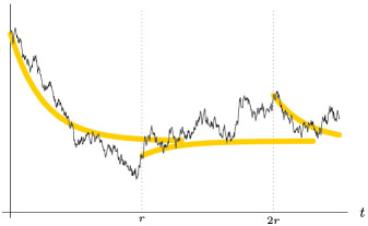
Figure 2: Splitting the process into fluid-scaled parts, starting at $0,r,2r,\ldots.$

7.1 Outline of the proof of Theorem 7.1.

The outline of the proof of Theorem 7.1 is as follows. We are interested in the dynamics of $\hat{\mathbf{q}}^{r}(t)$ over $t\in[0,T]$, that is, of $\mathbf{Q}^{r}(\tau)$ over $\tau\in[0,r^{2}T]$. We will split this time interval into $\lfloor rT\rfloor+1$ pieces starting at $0,r,2r,\ldots,$ and look at each piece under a fluid scaling. We will define a “good event” $\hat{E}_{r}$ under which the arrivals in all of the pieces are well behaved (Section 7.1.1). We then apply Theorem 4.3 to deduce that, under this event, the queue size process in each of the pieces can be (uniformly) approximated by a fluid model solution (Lemma 7.3). We then use the properties of the fluid model solution stated in Theorem 5.4 to show that in each of the pieces, the queue size is (uniformly) close to the set of invariant states (Lemmas 7.4 and 7.5). Figure 2 depicts the idea. Finally we show that $\mathbb{P}(\hat{E}_{r})\to 1$ (Lemma 7.6). The formal proof is given in Section 7.1.2.

Note that Lemmas 7.3–7.5 are all sample path-wise results that hold for every $\omega\in\hat{E}_{r}$, and so questions of independence etc. do not arise. The only part of the proof where probability comes in is Lemma 7.6.

The proof is written out for a single-hop switched network. For the multi-hop case, the argument holds verbatim; simply replace all references to the single-hop fluid limit Theorem 4.3 by references to the equivalent multi-hop result, and replace all references to the description of single-hop fluid model solutions in Theorem 5.4 by references to the multi-hop version Theorem 6.2.

7.1.1 The good event and the fluid-scaled pieces.

Define the fluid-scaled pieces $\tilde{x}^{r,m,z}(u)=(\tilde{\mathbf{q}}^{r,m,z}(u),\tilde{\mathbf{a}}^{r,m,z}(u),\tilde{\mathbf{y}}^{r,m,z}(u),\tilde{s}^{r,m,z}(u))$ of the original process by

$$\tilde{\mathbf{q}}^{r,m,z}(u) = \mathbf{Q}^{r}(rm+zu)/z,$$

$$\tilde{\mathbf{a}}^{r,m,z}(u) = \bigl{(}\mathbf{A}^{r}(rm+zu)-\mathbf{A}^{r}(rm)\bigr{)}/z,$$

$$\tilde{\mathbf{y}}^{r,m,z}(u) = \bigl{(}\mathbf{Y}^{r}(rm+zu)-\mathbf{Y}^{r}(rm)\bigr{)}/z,$$

$$\tilde{s}^{r,m,z}(u) = \bigl{(}S^{r}(rm+zu)-S^{r}(rm)\bigr{)}/z$$

for $0\leq m\leq\lfloor rT\rfloor$, $z\geq r$ and $u\geq 0$. Here $r$ indicates which process we are considering, $m$ indicates the piece and $z$ indicates the fluid-scaling parameter. The scaling parameter $z_{r,m}=|\mathbf{Q}^{r}(rm)|\vee r$ is particularly important, and for convenience we will define $\tilde{x}^{r,m}(u)=(\tilde{\mathbf{q}}^{r,m}(u),\tilde{\mathbf{a}}^{r,m}(u),\tilde{\mathbf{y}}^{r,m}(u),\tilde{s}^{r,m}(u))$ by

$$\tilde{\mathbf{q}}^{r,m}(u) = \tilde{\mathbf{q}}^{r,m,z_{r,m}}(u),\qquad\tilde{\mathbf{a}}^{r,m}(u)=\tilde{\mathbf{a}}^{r,m,z_{r,m}}(u),$$

$$\tilde{\mathbf{y}}^{r,m}(u) = \tilde{\mathbf{y}}^{r,m,z_{r,m}}(u),\qquad\tilde{s}^{r,m}(u)=\tilde{s}^{r,m,z_{r,m}}(u).$$

The good event is defined to be

$$\hat{E}_{r} = \Bigl{\{}\sup_{u\in[0,T^{\mathrm{fluid}}]}|\tilde{\mathbf{a}}^{r,m,w_{r,k}}(u)-\bolds{\lambda}^{r}u|<\eta_{r}\mbox{ for all $0\leq m\leq\lfloor rT\rfloor$}$$

$$\hskip 19.0pt\mbox{and $0\leq k\leq\lfloor Lr\log r\rfloor$, where $w_{r,k}=r(1+k/\log r)$}\Bigr{\}}.$$

By this, we mean that $\hat{E}_{r}$ is a subset of the sample space for the $r$th system, and we write $\tilde{x}^{r,m,w_{r,k}}(\cdot)(\omega)$ etc. for $\omega\in\hat{E}_{r}$ when we wish to emphasize the dependence on $\hat{E}_{r}$. The constants here are $T^{\mathrm{fluid}}=(2+\lambda^{\max}+NS^{\max})(H_{\zeta}+1)$, $\lambda^{\max}=\sup_{r}|\bolds{\lambda}^{r}|$, $\zeta>0$ is chosen as specified in Section 7.1.2 below, $H_{\zeta}$ is chosen as in Theorem 5.4(v), $L=1+T(1+\lambda^{\max}+NS^{\max})$, $S^{\max}=\max_{{\bolds{\pi}}\in\mathcal{S}}|{\bolds{\pi}}|$ and the sequence of deviation terms $\eta_{r}\in[0,1]$ is chosen as specified in Lemma 7.6 such that $\eta_{r}\to 0$ as $r\to\infty$.

Lemma 7.3.

Let $\operatorname{FMS}$ be the set of fluid model solutions over time horizon $[0,T^{\mathrm{fluid}}]$ for arrival rate vector $\bolds{\lambda}$, and let $\operatorname{FMS}(\mathbf{q}_{0})$ and $\operatorname{FMS}_{1}$ be as specified in Definition 4.1. Then

$$\sup_{\omega\in\hat{E}_{r}}\max_{0\leq m\leq\lfloor rT\rfloor}d(\tilde{x}^{r,m}(\cdot)(\omega),\operatorname{FMS}_{1})\to 0\qquad\mbox{as $r\to\infty$}$$ (50)

and

$$\sup_{\omega\in\hat{E}_{r}}d(\tilde{x}^{r,0}(\cdot)(\omega),\operatorname{FMS}(\mathbf{q}_{0}))\to 0\qquad\mbox{as $r\to\infty$},$$ (51)

where $\mathbf{q}_{0}=\hat{\mathbf{q}}_{0}/(|\hat{\mathbf{q}}_{0}|\vee 1)$.

The proof of each equation will use Theorem 4.3. We start with (50). The theorem requires the use of an index $j$ in some totally ordered countable set; here we shall use the pair $j\equiv(r,m)$ ordered lexicographically, where $r\in\mathbb{N}$ and $0\leq m\leq\lfloor rT\rfloor$. Lexicographic ordering means $(r,m)\geq(r^{\prime},m^{\prime})$ iff either $r>r^{\prime}$ or both $r=r^{\prime}$ and $m\geq m^{\prime}$. Note that $j\to\infty$ implies $r\to\infty$ (and vice versa).

To apply the theorem, we first need to pick constants. Let $K=1$, let $\bolds{\lambda}$ and $\bolds{\lambda}^{j}=\bolds{\lambda}^{r}\to\bolds{\lambda}$ as per Assumption 2.5 and let $\varepsilon_{j}=\eta_{r}(1+1/\log r)$ so that $\varepsilon_{j}\to 0$. Thus condition (23) of Theorem 4.3 is satisfied. Now let

$$G_{j}\equiv G_{r,m}=\{(\tilde{x}^{r,m}(\cdot)(\omega),z_{r,m}(\omega))\dvtx\omega\in\hat{E}_{r}\}.$$

It is worth stressing that $G_{j}\equiv G_{r,m}$ is a set of sample paths and associated scaling parameters, not a probabilistic event, and so any questions about the lack of independence between $\tilde{x}^{r,m}(\cdot)(\omega)$ and $z_{r,m}(\omega)$ are void. Note also that although the events $\hat{E}_{r}$ lie in different probability spaces for each $r$, this has no bearing on the definition of $G_{j}$ nor on the application of Theorem 4.3.

We next show that $G_{j}$ satisfies conditions (24)–(26) of Theorem 4.3, for $j$ sufficiently large. Equation (24) follows straightforwardly from the fact that $z_{r,m}\geq r$, hence $\inf\{z\dvtx(\tilde{x},z)\in G_{r,m}\}\geq r$, hence $\inf\{z\dvtx(\tilde{x},z)\in G_{j}\}\to\infty$. For (25), later in the proof we will establish that, under $\hat{E}_{r}$ for $r$ large enough,

$$\quad{\sup_{t\in[0,T^{\mathrm{fluid}}]}}|\tilde{\mathbf{a}}^{r,m}(t)-\bolds{\lambda}^{r}t|<\eta_{r}\biggl{(}1+\frac{1}{\log r}\biggr{)}\qquad\mbox{for all }0\leq m\leq\lfloor rT\rfloor,$$ (52)

which implies that for all $(\tilde{x},z)\in G_{j}\equiv G_{r,m}$, ${\sup_{t\in[0,T^{\mathrm{fluid}}]}}|\tilde{\mathbf{a}}^{j}(t)-\bolds{\lambda}^{j}t|<\varepsilon_{j}$ as required. Equation (26) follows straightforwardly from the scaling used to define $\tilde{\mathbf{q}}^{j}(0)\equiv\tilde{\mathbf{q}}^{r,m}(0)$: for every $\omega$, not merely $\omega\in\hat{E}_{r}$,

$$|\tilde{\mathbf{q}}^{r,m}(0)|=\biggl{|}\frac{\mathbf{Q}^{r}(rm)}{z_{r,m}}\biggr{|}=\biggl{|}\frac{\mathbf{Q}^{r}(rm)}{|\mathbf{Q}^{r}(rm)|\vee r}\biggr{|}\leq 1.$$

Since $G_{j}$ satisfies the conditions of Theorem 4.3 for sufficiently large $j$, we can apply that theorem to deduce

$$\sup_{(\tilde{x},z)\in G_{j}}d(\tilde{x},\operatorname{FMS}_{1})\to 0\qquad\mbox{as $j\to\infty$}.$$

Rewriting $j$ as $(r,m)$, and turning the limit statement into a $\limsup$ statement,

$$\sup_{(r^{\prime},m)\geq(r,0)}\sup_{(\tilde{x},z)\in G_{r^{\prime},m}}d(\tilde{x},\operatorname{FMS}_{1})\to 0\qquad\mbox{as $r\to\infty$}$$

and in particular

$$\max_{0\leq m\leq\lfloor rT\rfloor}\sup_{(\tilde{x},z)\in G_{r,m}}d(\tilde{x},\operatorname{FMS}_{1})\to 0\qquad\mbox{as $r\to\infty$.}$$

Rewriting $(\tilde{x},z)\in G_{r,m}$ in terms of $\omega\in\hat{E}_{r}$, as per the definition of $G_{r,m}$,

$$\max_{0\leq m\leq\lfloor rT\rfloor}\sup_{\omega\in\hat{E}_{r}}d(\tilde{x}^{r,m}(\cdot)(\omega),\operatorname{FMS}_{1})\to 0\qquad\mbox{as $r\to\infty$.}$$

Interchanging the $\max$ and the $\sup$ gives (50).

To establish (51), we will again apply Theorem 4.3 but this time using the index $j\equiv r$, $\bolds{\lambda}^{j}=\bolds{\lambda}^{r}\to\bolds{\lambda}$ and $\varepsilon_{j}=\eta_{r}(1+1/\log r)$ as above, and define

$$G_{j}\equiv G_{r}=\{(\tilde{x}^{r,0}(\cdot)(\omega),z_{r,0}(\omega))\dvtx\omega\in\hat{E}_{r}\}.$$

Equations (23)–(26) hold just as before. For (28), we will use $\mathbf{q}_{0}$ as in the statement of this lemma, and $\varepsilon^{\prime}_{j}=|\tilde{\mathbf{q}}^{r,0}(0)-\mathbf{q}_{0}|$. This is a well-defined constant (i.e., it does not depend on the randomness $\omega$), because we assumed in Theorem 7.1 that the initial queue sizes $\mathbf{Q}^{r}(0)$ are nonrandom, and by definition $\tilde{\mathbf{q}}^{r,0}(0)=\mathbf{Q}^{r}(0)/(|\mathbf{Q}^{r}(0)|\vee r)$. Furthermore, Theorem 7.1 assumes $\hat{\mathbf{q}}^{r}(0)\to\hat{\mathbf{q}}_{0}$, which implies $\tilde{\mathbf{q}}^{r,0}(0)\to\mathbf{q}_{0}$ hence $\varepsilon^{\prime}_{j}\to 0$. Equation (28) then follows straightforwardly, for every $\omega$ not merely $\omega\in\hat{E}_{r}$. Applying Theorem 4.3, we deduce that

$$\sup_{(\tilde{x},z)\in G_{j}}d(\tilde{x},\operatorname{FMS}(\mathbf{q}_{0}))\to 0\qquad\mbox{as $j\to\infty$}.$$

Equivalently,

$$\sup_{\omega\in\hat{E}_{r}}d(\tilde{x}^{r,0}(\cdot)(\omega),\operatorname{FMS}(\mathbf{q}_{0}))\to 0\qquad\mbox{as $r\to\infty$}$$

as required.

To complete the proof of Lemma 7.3, the only remaining claim that needs to be established is (52). We will proceed in two steps. First we prove that $|\mathbf{Q}^{r}(rm)|\leq Lr^{2}$ under $\hat{E}_{r}$, for $r$ sufficiently large and for all $0\leq m\leq\lfloor rT\rfloor$. To see this, note from (7) that

$$\mathbf{Q}^{r}(rm)\leq\mathbf{Q}^{r}(0)+\mathbf{A}^{r}(rm)+NrmS^{\max}.$$

Now $\hat{E}_{r}$ gives a suitable bound on arrivals: for all $0\leq m^{\prime}\leq\lfloor rT\rfloor$, and using the fact that $1\leq T^{\mathrm{fluid}}$,

$$\biggl{|}\frac{\mathbf{A}^{r}(rm^{\prime}+r)-\mathbf{A}^{r}(rm^{\prime})}{r}-\bolds{\lambda}^{r}\biggr{|}=|\tilde{\mathbf{a}}^{r,m^{\prime},w_{r,0}}(1)-\bolds{\lambda}^{r}|<\eta_{r},$$

and by applying this from $m^{\prime}=0$ to $m^{\prime}=m-1$ we find $|\mathbf{A}^{r}(rm)|\leq rm(\lambda^{\max}+\eta_{r})$. The assumptions of Theorem 7.1 tell us that $\mathbf{Q}^{r}(0)/r\to\hat{\mathbf{q}}_{0}$ for some $\hat{\mathbf{q}}_{0}\in\mathbb{R}_{+}^{N}$. Putting all this together, we find that for sufficiently large $r$

$$|\mathbf{Q}^{r}(rm)|\leq r^{2}\bigl{(}1+T(1+\lambda^{\max}+NS^{\max})\bigr{)}=Lr^{2}\qquad\mbox{for any }0\leq m\leq\lfloor rT\rfloor.$$

Now we proceed to prove (52), under $\hat{E}_{r}$ for $r$ sufficiently large. Observe that (for $r>2$) there exists $k\in\{1,\ldots,\lfloor Lr\log r\rfloor\}$ such that $w_{r,k-1}\leq z_{r,m}\leq w_{r,k}$; this follows from $r\leq z_{r,m}=|\mathbf{Q}^{r}(rm)|\vee r\leq Lr^{2}$ and the definition of $w_{r,k}$ in (7.1.1). Hence for any $t\in[0,T^{\mathrm{fluid}}]$,

$$|\tilde{\mathbf{a}}^{r,m}(t)-\bolds{\lambda}^{r}t|$$

$$\qquad=\biggl{|}\frac{\mathbf{A}^{r}(rm+z_{r,m}t)-\mathbf{A}^{r}(rm)}{z_{r,m}}-\bolds{\lambda}^{r}t\biggr{|}$$

$$\qquad=\biggl{|}\frac{\mathbf{A}^{r}(rm+w_{r,k}u)-\mathbf{A}^{r}(rm)}{w_{r,k}}-\bolds{\lambda}^{r}u\biggr{|}\biggl{(}\frac{w_{r,k}}{z_{r,m}}\biggr{)}\qquad\mbox{where $u=tz_{r,m}/w_{r,k}$}$$

$$\qquad=|\tilde{\mathbf{a}}^{r,m,w_{r,k}}(u)-\bolds{\lambda}^{r}u|\biggl{(}\frac{w_{r,k}}{z_{r,m}}\biggr{)}$$

$$\qquad<\eta_{r}\frac{w_{r,k}}{z_{r,m}}\qquad\mbox{since $\hat{E}_{r}$ holds and $u\leq t\leq T^{\mathrm{fluid}}$}$$

$$\qquad\leq\eta_{r}\frac{w_{r,k}}{w_{r,k-1}}\qquad\mbox{since $z_{r,m}\geq w_{r,k-1}$}$$

$$\qquad=\eta_{r}\biggl{(}1+\frac{1}{k-1+\log r}\biggr{)}\leq\eta_{r}\biggl{(}1+\frac{1}{\log r}\biggr{)}.$$

This establishes (52) and completes the proof.

Lemma 7.4 ((Choice of approximating piece)).

Given $t\in[0,T]$ and $r\in\mathbb{N}$, define $m^{*}=m^{*}(r,t)$ and $u^{*}=u^{*}(r,t)$ by

$$m^{*}=\min\{m\in\mathbb{Z}_{+}\dvtx rm\leq r^{2}t\leq rm+T^{\mathrm{fluid}}z_{r,m}\},\qquad u^{*}=\frac{r^{2}t-rm^{*}}{z_{r,m^{*}}}.$$

This is a sound definition (i.e., the set for $m^{*}$ is nonempty). Further, under event $\hat{E}_{r}$, either $m^{*}=0$ and $0\leq u^{*}\leq T^{\mathrm{fluid}}$, or $0<m^{*}\leq\lfloor rT\rfloor$ and $H_{\zeta}<u^{*}\leq T^{\mathrm{fluid}}$.

The set for $m^{*}$ is nonempty because $z_{r,m}\geq r$ and $T^{\mathrm{fluid}}\geq 1$. The upper bound for $m^{*}$ is trivial. The upper bound for $u^{*}$ in either case is trivial. To prove the lower bound for $u^{*}$ when $m^{*}>0$, $r^{2}t>r(m^{*}-1)+T^{\mathrm{fluid}}z_{r,m^{*}-1}$ due to the minimality of $m^{*}$. Hence

$$u^{*}=\frac{r^{2}t-rm^{*}}{z_{r,m^{*}}}>\frac{T^{\mathrm{fluid}}z_{r,m^{*}-1}-r}{z_{r,m^{*}}}\geq T^{\mathrm{fluid}}\frac{z_{r,m^{*}-1}}{z_{r,m^{*}}}-1.$$

To bound $z_{r,m^{*}-1}/z_{r,m^{*}}$, we can use (7) and the bound on $\mathbf{a}^{r,m,w_{r,0}}(1)$ provided by $\hat{E}_{r}$ to show that for any $m$

$$z_{r,m} = |\mathbf{Q}^{r}(rm)|\vee r$$

$$\leq \bigl{(}|\mathbf{Q}^{r}(rm-r)|+r(\lambda^{\max}+\eta_{r}+NS^{\max})\bigr{)}\vee r$$

$$\leq |\mathbf{Q}^{r}(rm-r)|\vee r+r(\lambda^{\max}+1+NS^{\max})\qquad\mbox{since $\eta_{r}\leq 1$}$$

$$\leq z_{r,m-1}(2+\lambda^{\max}+NS^{\max})\qquad\mbox{since $z_{r,m-1}\geq r$}.$$

Substituting this back into the earlier bound for $u^{*}$,

$$u^{*}>\frac{T^{\mathrm{fluid}}}{2+\lambda^{\max}+NS^{\max}}-1,$$

and this is equal to $H_{\zeta}$ by choice of $T^{\mathrm{fluid}}$.

Lemma 7.5 ((Pathwise multiplicative state space collapse)).

Let $0<\zeta<1$, $t\in[0,T]$ and $r\in\mathbb{N}$ be given. Suppose there exist $m\in\{0,\ldots,\lfloor rT\rfloor\}$, $u\in[0,T^{\mathrm{fluid}}]$ and $x\in\operatorname{FMS}$ such that $r^{2}t=rm+z_{r,m}u$ and $\|\tilde{x}^{r,m}-x\|<\zeta$, and furthermore either (i) $m>0$ and $u>H_{\zeta}$ and $x\in\operatorname{FMS}_{1}$, or (ii) $m=0$ and $x\in\operatorname{FMS}(\mathbf{q}_{0})$ where $\mathbf{q}_{0}$ is as defined in Lemma 7.3. Then

$$\quad\frac{|\hat{\mathbf{q}}^{r}(t)-\Delta W(\hat{\mathbf{q}}^{r}(t))|}{\|\hat{\mathbf{q}}^{r}(\cdot)\|\vee 1}\leq\frac{|\hat{\mathbf{q}}^{r}(t)-\Delta W(\hat{\mathbf{q}}^{r}(t))|}{z_{r,m}/r}<2\zeta+\operatorname{mc}_{\zeta}(\Delta W),$$ (53)

where $\operatorname{mc}_{\zeta}(\Delta W)$ is the modulus of continuity of the map $\mathbf{q}\mapsto\Delta W(\mathbf{q})$ over

$$\mathcal{D}=\{\mathbf{q}^{\prime}\in\mathbb{R}_{+}^{N}\dvtx|\mathbf{q}^{\prime}-\mathbf{q}|\leq 1\mbox{ for some $\mathbf{q}$ such that }L(\mathbf{q})\leq L(\mathbf{1})\}$$

for $L(\cdot)$ as in Definition 5.3.

The first inequality is trivially true because

$$\frac{z_{r,m}}{r}=\frac{|\mathbf{Q}^{r}(rm)|\vee r}{r}\leq\Bigl{(}\sup_{u\in[0,T]}\hat{\mathbf{q}}^{r}(u)\Bigr{)}\vee 1.$$

For the second inequality, note that after unwrapping the $\hat{\mathbf{q}}^{r}(\cdot)$ scaling and wrapping it up again in the $\tilde{\mathbf{q}}^{r,m}$ scaling, the middle term in (53) is

$$\mbox{MT}=|\tilde{\mathbf{q}}^{r,m}(u)-\Delta W(\tilde{\mathbf{q}}^{r,m}(u))|.$$

Writing $\mathbf{q}$ for the queue component of $x$,

MT $$\leq |\tilde{\mathbf{q}}^{r,m}(u)-\mathbf{q}(u)|+|\mathbf{q}(u)-\Delta W(\mathbf{q}(u))|+|\Delta W(\mathbf{q}(u))-\Delta W(\tilde{\mathbf{q}}^{r,m}(u))|$$

$$= \mbox{(\ref{equ52a})}+\mbox{(\ref{equ52b})}+\mbox{(\ref{equ52c})}\qquad\mbox{respectively}.$$

We can bound each term as follows:

(54b)

(54c)

(54e)

(54g)

(54h)

(54j)

Lemma 7.6 ((The good event has high probability)).

Under the assumptions of Theorem 7.1, $\mathbb{P}(\hat{E}_{r})\to 1$ as $r\to\infty$. The deviation terms are given by $\eta_{r}=\min(1,\sup_{z\geq r}T^{\mathrm{fluid}}\delta_{\lfloor zT^{\mathrm{fluid}}\rfloor})$ and $\eta_{r}\to 0$ as $r\to\infty$.

By a simple union bound, and then using the fact that the arrival process has stationary increments,

$$\mathbb{P}(\hat{E}_{r}) \geq 1-\sum_{m=0}^{\lfloor rT\rfloor}\sum_{k=0}^{\lfloor Lr\log r\rfloor}\mathbb{P}\Bigl{(}{\sup_{u\in[0,T^{\mathrm{fluid}}]}}|\tilde{\mathbf{a}}^{r,m,w_{r,k}}(u)-\bolds{\lambda}^{r}u|\geq\eta_{r}\Bigr{)}$$

$$= 1-(1+\lfloor rT\rfloor)\sum_{k=0}^{\lfloor Lr\log r\rfloor}\mathbb{P}\Bigl{(}{\sup_{u\in[0,T^{\mathrm{fluid}}]}}|\tilde{\mathbf{a}}^{r,0,w_{r,k}}(u)-\bolds{\lambda}^{r}u|\geq\eta_{r}\Bigr{)}$$

$$= 1-(1+rT)\sum_{k=0}^{\lfloor Lr\log r\rfloor}\mathbb{P}\biggl{(}\sup_{u\in[0,T^{\mathrm{fluid}}]}\biggl{|}\frac{A^{r}(w_{r,k}u)}{w_{r,k}}-\bolds{\lambda}^{r}u\biggr{|}\geq\eta_{r}\biggr{)}.$$

To bound this we will use Assumption 2.5, which says that

$$z(\log z)^{2}\mathbb{P}\biggl{(}\sup_{\tau\leq z}\frac{1}{z}|\mathbf{A}^{r}(\tau)-\bolds{\lambda}^{r}\tau|\geq\delta_{z}\biggr{)}\to 0\qquad\mbox{as $z\to\infty$}$$

uniformly in $r$. After extending the domain of $\mathbf{A}^{r}$ to $\mathbb{R}_{+}$ by linear interpolation in each interval $(\tau,\tau+1)$, and extending the domain of $\delta_{z}$ to $z\in\mathbb{R}_{+}$ by $\delta(z)=\delta_{\lfloor z\rfloor}\vee\delta_{\lceil z\rceil}$, and rescaling $z$ by $T^{\mathrm{fluid}}$,

$$z(\log z)^{2}\mathbb{P}\biggl{(}\sup_{u\in[0,T^{\mathrm{fluid}}]}\biggl{|}\frac{\mathbf{A}^{r}(zu)}{z}-\bolds{\lambda}^{r}u\biggr{|}\geq T^{\mathrm{fluid}}\delta(zT^{\mathrm{fluid}})\biggr{)}\to 0\qquad\mbox{as $z\to\infty$}$$

uniformly in $r$. In other words, for any $\phi>0$ there exists $z_{0}$ such that for all $z\geq z_{0}$ and all $r$,

$$\mathbb{P}\biggl{(}\sup_{u\in[0,T^{\mathrm{fluid}}]}\biggl{|}\frac{\mathbf{A}^{r}(zu)}{z}-\bolds{\lambda}^{r}u\biggr{|}\geq T^{\mathrm{fluid}}\delta(zT^{\mathrm{fluid}})\biggr{)}<\frac{\phi}{z(\log z)^{2}}.$$

Now pick $r_{0}$ sufficiently large that $r_{0}\geq z_{0}$ and $\sup_{z\geq r_{0}}T^{\mathrm{fluid}}\delta(zT^{\mathrm{fluid}})<1$, which we can do since $\delta(z)\to 0$ as $z\to\infty$ by Assumption 2.5. This choice implies that for any $r\geq r_{0}$ and $z\geq r$, $T^{\mathrm{fluid}}\delta(zT^{\mathrm{fluid}})\leq\eta_{r}$ [recall that $\eta_{r}=\min(1,\sup_{z\geq r}T^{\mathrm{fluid}}\delta_{\lfloor zT^{\mathrm{fluid}}\rfloor})$]. Hence, for any $r\geq r_{0}$ and $z\geq r$,

$$\mathbb{P}\biggl{(}\sup_{u\in[0,T^{\mathrm{fluid}}]}\biggl{|}\frac{\mathbf{A}^{r}(zu)}{z}-\bolds{\lambda}^{r}u\biggr{|}\geq\eta_{r}\biggr{)}<\frac{\phi}{z(\log z)^{2}}.$$

Applying this bound to $\mathbb{P}(\hat{E}_{r})$, and using the facts that $w_{r,k}\geq r$ and$w_{r,k}(\log w_{r,k})^{2}\geq r(1+k/\log r)(\log r)^{2}$,

$$1-\mathbb{P}(\hat{E}_{r}) < \phi\biggl{(}\frac{1+\lfloor rT\rfloor}{r(\log r)^{2}}\biggr{)}\sum_{k=0}^{\lfloor Lr\log r\rfloor}\frac{1}{1+k/\log r}$$

$$= \phi\biggl{(}\frac{1+\lfloor rT\rfloor}{r\log r}\biggr{)}\sum_{k=0}^{\lfloor Lr\log r\rfloor}\frac{1}{k+\log r}$$

$$\leq \phi\biggl{(}\frac{1+\lfloor rT\rfloor}{r\log r}\biggr{)}\int_{\ell=0}^{\lfloor Lr\log r\rfloor}\frac{1}{\ell-1+\log r}\,d\ell$$

$$= \phi\biggl{(}\frac{1+\lfloor rT\rfloor}{r\log r}\biggr{)}\log\biggl{(}1+\frac{\lfloor Lr\log r\rfloor}{\log r-1}\biggr{)}.$$

The final expression converges to $\phi T$ as $r\to\infty$. Since $\phi$ can be chosen arbitrarily small, $\mathbb{P}(\hat{E}_{r})\to 1$ as $r\to\infty$.

7.1.2 Proof of Theorem 7.1.

Given $\delta>0$, pick $\zeta>0$ such that $2\zeta+\operatorname{mc}_{\zeta}(\Delta W)<\delta\wedge 1$ where $\operatorname{mc}_{\zeta}(\Delta W)$ is the modulus of continuity of $\Delta W$ over the set $\mathcal{D}$ specified in Lemma 7.5. We can achieve the desired bound by making $\zeta$ sufficiently small; this is because $\Delta W$ is continuous, hence uniformly continuous on compact sets, and $\mathcal{D}$ is compact as a consequence of Theorem 5.4(i), hence $\operatorname{mc}_{\zeta}(\Delta W)\to 0$ as $\zeta\to 0$. With this choice of $\zeta$, define the good sets $\hat{E}_{r}$ and the constants $T^{\mathrm{fluid}}$ and $H_{\zeta}$ as specified by (7.1.1).

By Lemma 7.3, there exists $r_{0}$ such that for $r\geq r_{0}$ and for all $\omega\in\hat{E}_{r}$ and all $m$, $d(\tilde{x}^{r,m},\operatorname{FMS}_{1})<\zeta$ and $d(\tilde{x}^{r,0},\operatorname{FMS}(\mathbf{q}_{0}))<\zeta$, where $\mathbf{q}_{0}$ is defined in the statement of the lemma.

Now, pick any $t\in[0,T^{\mathrm{fluid}}]$ and $r\geq r_{0}$, and assume $\hat{E}_{r}$ holds. Lemma 7.4 says that we can choose $m\in\{0,\ldots,\lfloor rT\rfloor\}$ and $u\in[0,T^{\mathrm{fluid}}]$ such that $r^{2}t=rm+z_{r,m}u$, and furthermore either (i) $m>0$ and $u>H_{\zeta}$ or (ii) $m=0$. By Lemma 7.3, we can pick $x\in\operatorname{FMS}$ (depending on $r$, $t$ and the $\omega$) such that $\|\tilde{x}^{r,m}-x\|<\zeta$ and furthermore either (i) $m>0$ and $x\in\operatorname{FMS}_{1}$ or (ii) $m=0$ and $x\in\operatorname{FMS}(\mathbf{q}_{0})$. Then, by Lemma 7.5,

$$\frac{|\hat{\mathbf{q}}^{r}(t)-\Delta W(\hat{\mathbf{q}}^{r}(t))|}{\|\hat{\mathbf{q}}^{r}(\cdot)\|\vee 1}<\delta.$$

This bound holds for every $t\in[0,T]$ and $r\geq r_{0}$, in a sample path-wise sense, whenever $\omega\in\hat{E}_{r}$.

Finally, Lemma 7.6 says that $\mathbb{P}(\hat{E}_{r})\to 1$. This completes the proof. $\Box$

8 An optimal policy?

Our motivation for this work was Conjecture 3.1, which says that for an input-queued switch the performance of MW-$\alpha$ improves as $\alpha\searrow 0$. We have not been able to prove this. However, under a condition on the arrival rate, we can show (i) that the critically-loaded fluid model solutions for a single-hop switched network approach optimal (in the sense of minimizing total amount of work in the network) as $\alpha\searrow 0$; and (ii) that for an input-queued switch the set of invariant states $\mathcal{I}$ defined in Section 7 is sensitive to $\alpha$. We speculate that these findings might eventually form part of a proof of a heavy traffic limit theorem supporting Conjecture 3.1, given that critically loaded fluid models and invariant states play an important role in heavy traffic theorems.

In this section we state the condition on the arrival rates, and give the results (i) and (ii). Motivated by these results, we make a conjecture about an optimal scheduling policy.

Definition 8.1 ((Complete loading)).

Consider a switched network with arrival rate vector $\bolds{\lambda}$. Say that $\bolds{\lambda}$ satisfies the complete loading condition if $\bolds{\lambda}\in\Lambda$, and there is a convex combination of critically loaded virtual resources that gives equal weight to each queue; in other words if

$$\frac{\mathbf{1}}{\max_{{\bolds{\pi}}\in\mathcal{S}}\mathbf{1}\cdot{\bolds{\pi}}}\in\langle{\Xi(\bolds{\lambda})}\rangle.$$

Theorem 8.2 ((Near-optimality of fluid models under complete loading)).

Consider a single-hop switched network with arrival rate vector $\bolds{\lambda}\in\Lambda$.

For any fluid model solution for the MW-$\alpha$ policy, $\mathbf{1}\cdot\mathbf{q}(t)\leq\break N^{\alpha/(1+\alpha)}\mathbf{1}\cdot\mathbf{q}(0)$.

For any fluid model solution for any scheduling policy, if $\bolds{\lambda}$ satisfies the complete loading condition, then $\mathbf{1}\cdot\mathbf{q}(t)\geq\mathbf{1}\cdot\mathbf{q}(0)$.

The first claim relies on the standard result that for any $\mathbf{x}\in\mathbb{R}_{+}^{N}$ and $\beta>1$,

$$\frac{1}{{N}^{1-1/\beta}}\sum_{n}x_{n}\leq\biggl{(}\sum_{n}x_{n}^{\beta}\biggr{)}^{1/\beta}\leq\sum_{n}x_{n}.$$ (55)

Using the Lyapunov function from Definition 5.3,

$$\mathbf{1}\cdot\mathbf{q}(t) \leq {N}^{1-1/(1+\alpha)}\biggl{(}\sum_{n}q_{n}(t)^{1+\alpha}\biggr{)}^{1/(1+\alpha)}\qquad\mbox{by the first inequality in (\ref{eq:holder2})}$$

$$= {N}^{\alpha/(1+\alpha)}L(\mathbf{q}(t))^{1/(1+\alpha)}\qquad\mbox{by definition of $L(\cdot)$}$$

$$\leq {N}^{\alpha/(1+\alpha)}L(\mathbf{q}(0))^{1/(1+\alpha)}\qquad\mbox{since $\dot{L}(\mathbf{q}(t))\leq 0$ by Theorem \ref{thm:fp}(i)}$$

$$\leq N^{\alpha/(1+\alpha)}\mathbf{1}\cdot\mathbf{q}(0)\qquad\mbox{by the second inequality in (\ref{eq:holder2}).}$$

The second claim is a simple consequence of Lemma 5.10. (This lemma is for a single-hop network. The multi-hop version, Lemma 6.8, does not have such a simple interpretation.)

Theorem 8.3 (($\mathcal{I}$ is sensitive to $\alpha$ for an input-queued switch)).

Consider an $M\times M$ input-queued switch running MW-$\alpha$, as introduced in Section 2.4. Let $\lambda_{ij}$ be the arrival rate at the queue at input port $i$ of packets destined for output port $j$, $\bolds{\lambda}\in\mathbb{R}_{+}^{M\times M}$. Suppose that $\bolds{\lambda}>\mathbf{0}$ componentwise, and furthermore that every input port and every output port is critically loaded, that is,

$$\sum_{j=1}^{M}\lambda_{{\hat{\imath}}j}=1\quad\mbox{and}\quad\sum_{i=1}^{M}\lambda_{i{\hat{\jmath}}}=1\qquad\mbox{for every }1\leq{\hat{\imath}},{\hat{\jmath}}\leq M.$$ (56)

Then $\bolds{\lambda}$ satisfies the complete loading condition, and the critically loaded virtual resources are

$$\Xi(\bolds{\lambda})=\{\mathbf{r}_{\hat{\imath}}\mbox{ for all }1\leq{\hat{\imath}}\leq M\}\cup\{\mathbf{c}_{\hat{\jmath}}\mbox{ for all }1\leq{\hat{\jmath}}\leq M\},$$

where $\mathbf{r}_{\hat{\imath}}$ and $\mathbf{c}_{\hat{\jmath}}$ are the row and column indicator matrices, $(\mathbf{r}_{\hat{\imath}})_{i,j}=1_{i={\hat{\imath}}}$ and $(\mathbf{c}_{\hat{\jmath}})_{i,j}=1_{j={\hat{\jmath}}}$. Define the workload map $W\dvtx\mathbb{R}_{+}^{M\times M}\to\mathbb{R}_{+}^{2M}$ by $W(\mathbf{q})=[{\bolds{\xi}}\cdot\mathbf{q}]_{{\bolds{\xi}}\in\Xi(\bolds{\lambda})}$. Denoting the invariant set by $\mathcal{I}(\alpha)$:

if $w$ is in the relative interior of $\{W(\mathbf{q})\dvtx\mathbf{q}\in\mathbb{R}_{+}^{M\times M}\}$, then $w$ is in $\{W(\mathbf{q})\dvtx\mathbf{q}\in\mathcal{I}(\alpha)\}$ for sufficiently small $\alpha>0$;

for a $2\times 2$ input-queued switch, $\{W(\mathbf{q})\dvtx\mathbf{q}\in\mathcal{I}(\alpha)\}$ is strictly increasing as $\alpha\searrow 0$.

Item (i) essentially says that $W(\mathcal{I}(\alpha))$ becomes as large as possible as $\alpha\searrow 0$, except for some possible issues at the boundary. We have only been able to prove (ii) for a $2\times 2$ switch, but we believe it holds for any $M\times M$ switch. The proofs are rather long, and depend on the specific structure of the input-queued switch, so they are left to the Appendix.

Conjecture 3.1 claims that, for an input-queued switch, performance improves as $\alpha\searrow 0$. Examples due to Ji, Athanasopoulou and Srikant srikantsmallswitch and Stolyar (personal communication) show that this is not true for general switched networks. However, Theorem 8.2 suggests that the conjecture might apply not just to input-queued switches but also to generalized switches under the complete loading condition; the examples of Ji, Athanasopoulou and Srikant srikantsmallswitch and Stolyar do not satisfy this condition. We therefore extend Conjecture 3.1 as follows.

Conjecture 8.4.

Consider a general single-hop switched network as described in Section 2, running MW-$\alpha$. Consider the diffusion scaling limit (described in Conjecture 7.2), and let $\bolds{\lambda}$ be the limiting arrival rates; assume $\bolds{\lambda}$ satisfies the complete loading condition. For every $\alpha>0$ there is a limiting stationary queue size distribution. The expected value of the sum of queue sizes under this distribution is nonincreasing as $\alpha\searrow 0$.

Theorem 8.2 says that MW-$\alpha$ approaches optimal as $\alpha\searrow 0$, under the complete loading condition. It is natural to ask if there is a policy that is optimal, rather than just a sequence of policies that approach optimal. Given that MW-$\alpha$ chooses a schedule ${\bolds{\pi}}$ to maximize ${\bolds{\pi}}\cdot\mathbf{q}^{\alpha}$ (where the exponent is taken componentwise), and since

$$x^{\alpha}=\cases{1+\alpha\log x+O(\alpha^{2}),&\quad if $x>0$,\cr 0,&\quad if $x=0$,}$$

we propose the following formal limit policy, which we call MSMW-log: at each time step, look at all maximum-size schedules, that is, those ${\bolds{\pi}}\in\mathcal{S}$ for which $\sum_{n}\pi_{n}1_{Q_{n}>0}$ is maximal. Among these, pick one which has maximal log-weight, that is, for which $\sum_{n\dvtx Q_{n}>0}\pi_{n}\log Q_{n}$ is maximal, breaking ties randomly.

Conjecture 8.5.

Consider a general single-hop switched network running MSMW-log. Consider the diffusion scaling limit, and let $\bolds{\lambda}$ be the limiting arrival rates; assume $\bolds{\lambda}$ satisfies the complete loading condition. There is a limiting stationary queue size distribution. This distribution minimizes the expected value of the sum of the queue sizes, over all scheduling policies for which this expected value is defined.

Scheduling policies based on MW are computationally difficult to implement because there are so many comparisons to be made. In future work we plan to investigate whether the techniques described in this paper can be applied to policies that may have worse performance but simpler implementation.

Appendix: Results for input-queued switches

In this section we prove Theorem 8.3. Throughout this Appendix we are considering a $M\times M$ input-queued switch. The set of schedules $\mathcal{S}$ consists of all $M\times M$ permutation matrices. We assume the arrival rate matrix $\bolds{\lambda}$ satisfies the complete loading condition (56) and that $\bolds{\lambda}>\mathbf{0}$ componentwise. We let the scheduling algorithm be MW-$\alpha$, and define $\mathcal{I}(\alpha)$ to be the set of invariant states.

.1 Identifying $\Lambda$, $\mathcal{S}^{*}$, $\Xi$ and $\Xi^{+}$.

The Birkhoff–von Neumann decomposition result says that a matrix is doubly substochastic if and only if it is less than or equal to a convex combination of permutation matrices, which yields

$$\Lambda=\Biggl{\{}\bolds{\lambda}\in[0,1]^{M\times M}\dvtx\sum_{j=1}^{M}\lambda_{{\hat{\imath}},j}\leq 1\mbox{ and }\sum_{i=1}^{M}\lambda_{i,{\hat{\jmath}}}\leq 1\mbox{ for all ${\hat{\imath}},{\hat{\jmath}}$}\Biggr{\}}.$$

Since $\bolds{\lambda}$ satisfies the complete loading condition (56), $\bolds{\lambda}\in\Lambda$.

Lemma .1 below gives $\mathcal{S}^{*}$, the set of virtual resources, that is, maximal extreme points of the set of feasible solutions to $()$. From the complete loading condition, it is clear that $\Xi(\bolds{\lambda})=\mathcal{S}^{*}$ as claimed in the theorem. It will also be useful, for the proof of Theorem 8.3(i), to identify $\Xi^{+}(\bolds{\lambda})$ as defined by (34). We claim that

$$\Xi^{+}(\bolds{\lambda})=\Xi(\bolds{\lambda}).$$ (57)

To see this, suppose ${\bolds{\xi}}$ is a nonmaximal extreme point of the set of feasible solutions to $()$; then there exists some other extreme point ${\bolds{\zeta}}$ such that ${\bolds{\xi}}\leq{\bolds{\zeta}}$ and ${\bolds{\xi}}\neq{\bolds{\zeta}}$; but because $\bolds{\lambda}>\mathbf{0}$ componentwise it must be that ${\bolds{\xi}}\cdot\bolds{\lambda}<{\bolds{\zeta}}\cdot\bolds{\lambda}$. We have found that $\bolds{\lambda}\in\Lambda$, so the solution to $()$ is $\leq 1$, hence ${\bolds{\xi}}\cdot\bolds{\lambda}<1$. Therefore ${\bolds{\xi}}\notin\Xi^{+}(\bolds{\lambda})$, that is, $\Xi^{+}(\bolds{\lambda})$ consists only of maximal extreme points.

Lemma .1.

The set of maximal extreme points of the set

$$F=\{{\bolds{\xi}}\in\mathbb{R}_{+}^{M\times M}\dvtx{\bolds{\xi}}\cdot{\bolds{\pi}}\leq 1\mbox{ for all }{\bolds{\pi}}\in\mathcal{S}\}$$

is given by

$$\mathcal{S}^{*}=\{\mathbf{r}_{\hat{\imath}}\mbox{ for all $1\leq{\hat{\imath}}\leq M$}\}\cup\{\mathbf{c}_{\hat{\jmath}}\mbox{ for all $1\leq{\hat{\jmath}}\leq M$}\},$$

where the row and column indicator matrices $\mathbf{r}_{\hat{\imath}}$ and $\mathbf{c}_{\hat{\jmath}}$ are defined by $(\mathbf{r}_{\hat{\imath}})_{i,j}=1_{i={\hat{\imath}}}$ and $(\mathbf{c}_{\hat{\jmath}})_{i,j}=1_{j={\hat{\jmath}}}$.

First we argue that every ${\bolds{\xi}}\in\mathcal{S}^{*}$ is a maximal extreme point of $F$. It is simple to check that ${\bolds{\xi}}\in F$. Also, ${\bolds{\xi}}$ is extreme because $F\subset[0,1]^{M\times M}$. Finally, ${\bolds{\xi}}$ is maximal because if it were not then there would be some $\bolds{\varepsilon}\geq\mathbf{0}$, $\bolds{\varepsilon}\neq\mathbf{0}$, such that ${\bolds{\xi}}+\bolds{\varepsilon}\in F$; but for any such $\bolds{\varepsilon}$ there is a matching ${\bolds{\pi}}$ such that $\bolds{\varepsilon}\cdot{\bolds{\pi}}>0$ hence ${\bolds{\xi}}+\bolds{\varepsilon}\notin F$.

Next we argue the converse, that all maximal extreme points of $F$ are in $\mathcal{S}^{*}$. The first step is to characterize the extreme points of $F$. We claim that if ${\bolds{\zeta}}\in F$, then it can be written ${\bolds{\zeta}}\leq{\bolds{\xi}}$ for some ${\bolds{\xi}}\in\langle{\mathcal{S}^{*}}\rangle$. Consider the optimization problem

$$\mbox{minimize }\sum_{{\hat{\imath}}=1}^{M}x_{\hat{\imath}}+\sum_{{\hat{\jmath}}=1}^{M}y_{\hat{\jmath}}\quad\mbox{over}\quad x_{\hat{\imath}}\geq 0,y_{\hat{\jmath}}\geq 0\qquad\mbox{for all }{\hat{\imath}},{\hat{\jmath}}$$

(58)

$$\mbox{such that }{\bolds{\zeta}}\leq\sum_{\hat{\imath}}x_{\hat{\imath}}\mathbf{r}_{\hat{\imath}}+\sum_{\hat{\jmath}}y_{\hat{\jmath}}\mathbf{c}_{\hat{\jmath}}.$$

The dual of this problem is

$$\mbox{maximize }\mathbf{a}\cdot{\bolds{\zeta}}\quad\mbox{over}\quad\mathbf{a}\in\mathbb{R}_{+}^{M\times M}$$

(59)

$$\mbox{such that }\mathbf{a}\cdot\mathbf{r}_{\hat{\imath}}\leq 1,\qquad\mathbf{a}\cdot\mathbf{c}_{\hat{\jmath}}\leq 1\qquad\mbox{for all }{\hat{\imath}},{\hat{\jmath}}.$$

[These problems are just $\operatorname{PRIMAL}({\bolds{\zeta}})$ and $()$, resp., but with respect to the “virtual” schedule set $\mathcal{S}^{*}$ rather than the actual schedule set $\mathcal{S}$.] By Slater’s condition, strong duality holds. Now, any matrix $\mathbf{a}$ that is feasible for (.1) is nonnegative and doubly substochastic, hence by the Birkhoff–von Neumann decomposition result it can be written as a $\mathbf{a}\leq\mathbf{b}$ where $\mathbf{b}$ is a convex combination of permutation matrices, that is, $\mathbf{b}\in\langle{\mathcal{S}}\rangle$. But by the assumption that ${\bolds{\zeta}}\in F$, ${\bolds{\zeta}}\cdot{\bolds{\pi}}\leq 1$ for all ${\bolds{\pi}}\in\mathcal{S}$, hence $\mathbf{b}\cdot{\bolds{\zeta}}\leq 1$, hence $\mathbf{a}\cdot{\bolds{\zeta}}\leq 1$, so the value of the optimization problem (.1) is $\leq 1$. By strong duality, the value of the optimization problem (.1) is also $\leq 1$. Therefore ${\bolds{\zeta}}\leq{\bolds{\xi}}$ for some ${\bolds{\xi}}\in\langle{\mathcal{S}}\rangle$.

We now claim that if ${\bolds{\zeta}}\in F$ then it can be written ${\bolds{\zeta}}=\sum_{\bolds{\xi}}a_{\bolds{\xi}}{\bolds{\xi}}$ where the sum is over some finite collection of values drawn from the set

$$E=\{{\bolds{\xi}}\in\mathbb{R}_{+}^{M\times M}\dvtx{\bolds{\xi}}\leq\mathbf{r}_{\hat{\imath}}\mbox{ or }{\bolds{\xi}}\leq\mathbf{c}_{\hat{\jmath}}\mbox{ for some }{\hat{\imath}},{\hat{\jmath}}\},$$

and all $a_{\bolds{\xi}}$ are $\geq 0$. We have just shown that

$${\bolds{\zeta}}=\sum_{\bolds{\xi}}a_{\bolds{\xi}}{\bolds{\xi}}-\mathbf{z}\qquad\mbox{for some }\mathbf{z}\geq\mathbf{0}\mbox{ and }a_{\bolds{\xi}}\geq 0,\qquad{\bolds{\xi}}\in E.$$ (60)

If $\mathbf{z}=\mathbf{0}$ we are done. Otherwise, pick some $(k,l)$ such that $z_{k,l}>0$ and define $\mathbf{n}^{k,l}$ by $(\mathbf{n}^{k,l})_{i,j}=1-1_{i=k\mbox{ and }j=l}$. Noting that $\sum a_{\bolds{\xi}}\xi_{k,l}\geq z_{k,l}>0$, we can rewrite ${\bolds{\zeta}}$ as

$${\bolds{\zeta}}=\frac{z_{k,l}}{\sum a_{\bolds{\xi}}\xi_{k,l}}\sum a_{\bolds{\xi}}{\bolds{\xi}}+\biggl{(}1-\frac{z_{k,l}}{\sum a_{\bolds{\xi}}\xi_{k,l}}\biggr{)}\sum a_{\bolds{\xi}}{\bolds{\xi}}\mathbf{n}^{k,l}-\mathbf{z}\mathbf{n}^{k,l},$$

where matrix multiplication is componentwise as per the notation specified in Section 1. We have thus rewritten ${\bolds{\zeta}}$ in the form (60), but now $\mathbf{z}$ has one fewer nonzero element. Continuing in this way we can remove all nonzero elements of $\mathbf{z}$, until we are left with ${\bolds{\zeta}}\in\langle{E}\rangle$.

We have therefore shown that all extreme points of $F$ are in $E$. Clearly, all maximal points of $E$ are in $\mathcal{S}^{*}$. Therefore, all the maximal extreme points of $F$ are in $\mathcal{S}^{*}$ as claimed.

.2 Proof of Theorem 8.3(i).

We first state two lemmas which will be needed in the proof. The first is a general closure property of permutation matrices, and the second is a property of invariant states of MW-$\alpha$. We then prove the theorem and the two lemmas.

Lemma .2.

Let $\mathbf{x}\in\mathbb{R}_{+}^{M\times M}$, and define $\mathbf{A}\in\mathbb{R}_{+}^{M\times M}$ by $A_{i,j}=1$ if there is some matching ${\bolds{\rho}}\in\mathcal{S}$ whose weight ${\bolds{\rho}}\cdot\mathbf{x}$ is maximal (i.e., ${\bolds{\rho}}\cdot\mathbf{x}=\max_{\bolds{\sigma}\in\mathcal{S}}\bolds{\sigma}\cdot\mathbf{x}$) and for which $\rho_{i,j}=1$; and $A_{i,j}=0$ otherwise. Then, for any matching ${\bolds{\pi}}$ such that

$$\pi_{i,j}=1\quad\Longrightarrow\quad A_{i,j}=1,$$

${\bolds{\pi}}$ is itself a maximum weight matching.

Lemma .3.

Fix any $\bolds{\lambda}\in\Lambda$, and any $\mathbf{q}\in\mathcal{I}(\alpha)$. For every $1\leq i,j\leq M$ such that $\lambda_{i,j}>0$, there exists a matching ${\bolds{\pi}}\in\mathcal{S}$ whose weight ${\bolds{\pi}}\cdot\mathbf{q}^{\alpha}$ is maximal (i.e., ${\bolds{\pi}}\cdot\mathbf{q}^{\alpha}=\max_{\bolds{\sigma}\in\mathcal{S}}\bolds{\sigma}\cdot\mathbf{q}^{\alpha}$, where the exponent is taken componentwise) and for which $\pi_{i,j}=1$.

Proof of Theorem 8.3(i) Suppose the claim of the theorem is not true, that is, that there exists a sequence $\alpha\searrow 0$ such that $w\notin\mathcal{W}(\alpha)=\{W(\mathbf{q})\dvtx\mathbf{q}\in\mathcal{I}(\alpha)\}$ for each $\alpha$ in the sequence.

Write $w=(w_{1\cdot},\ldots,w_{M\cdot},w_{\cdot 1},\ldots,w_{\cdot M})$, and define the function $\Delta^{\alpha}\dvtx\mathbb{R}_{+}^{2M}\to\mathbb{R}_{+}^{M\times M}$ to give the (unique) solution to the optimization problem

$$\mbox{minimize }\frac{1}{1+\alpha}\sum_{i,j}q_{i,j}^{1+\alpha}\quad\mbox{over}\quad\mathbf{q}\in\mathbb{R}_{+}^{M\times M}$$

$$\mbox{such that }\mathbf{r}_{\hat{\imath}}\cdot\mathbf{q}\geq w_{{\hat{\imath}}\cdot}\quad\mbox{and}\quad\mathbf{c}_{\hat{\jmath}}\cdot\mathbf{q}\geq w_{\cdot{\hat{\jmath}}}\qquad\mbox{for all }1\leq{\hat{\imath}},{\hat{\jmath}}\leq M.$$

This is the optimization problem defined in (35); we have simply written out $\Xi^{+}(\bolds{\lambda})$ explicitly using (57). By Lemma 5.6, the map $\Delta{W}\dvtx\mathbb{R}_{+}^{M\times M}\to\mathbb{R}_{+}^{M\times M}$ that defines $\mathcal{I}(\alpha)$ is simply the composition of $W\dvtx\mathbb{R}_{+}^{M\times M}\to\mathbb{R}_{+}^{2M}$ and $\Delta^{\alpha}\dvtx\mathbb{R}_{+}^{2M}\to\mathbb{R}_{+}^{M\times M}$. Let $\mathbf{q}(\alpha)=\Delta^{\alpha}(w)$. Note that $\mathbf{q}(\alpha)\in\mathcal{I}(\alpha)$; this is because $\mathbf{q}(\alpha)$ is optimal for $\Delta^{\alpha}(w)$, therefore it is optimal for $\Delta^{\alpha}(W(\mathbf{q}(\alpha)))$ which has a smaller feasible region, therefore $\mathbf{q}(\alpha)=\Delta^{\alpha}(W(\mathbf{q}(\alpha)))=\break\Delta{W}(\mathbf{q}(\alpha))$, that is, $\mathbf{q}(\alpha)\in\mathcal{I}(\alpha)$.

We next establish this claim: that for each $\alpha$ in the sequence, there exists $i$, $j$, $i^{\prime}$ and $j^{\prime}$ such that $q_{i,j}(\alpha)=0$, $q_{i^{\prime},j}(\alpha)\geq w_{\cdot j}/M$ and $q_{i,j^{\prime}}(\alpha)\geq w_{i\cdot}/M$. To prove this claim, observe that $W(\mathbf{q}(\alpha))\geq w$ by the constraints of the optimization problem $\Delta^{\alpha}$; and that $\mathbf{q}(\alpha)\in\mathcal{I}(\alpha)$ hence $W(\mathbf{q}(\alpha))\in\mathcal{W}(\alpha)$; hence $W(\mathbf{q}(\alpha))\neq w$ by assumption that $w\notin\mathcal{W}(\alpha)$. Therefore $W(\mathbf{q}(\alpha))>w$ in some component, that is, there is some $i$ or $j$ such that $\mathbf{r}_{i}\cdot\mathbf{q}(\alpha)>w_{i\cdot}$ or $\mathbf{c}_{j}\cdot\mathbf{q}(\alpha)>w_{\cdot j}$. Indeed, there must be both such an $i$ and $j$, since otherwise the sum of row workloads and column workloads would not be equal. Therefore $q_{i,j}(\alpha)=0$, since if $q_{i,j}(\alpha)>0$, then we could reduce $q_{i,j}(\alpha)$ and still have a feasible solution to the problem that defines $\Delta^{\alpha}(w)$ but with a smaller value of the objective function, which contradicts optimality of $\mathbf{q}(\alpha)$. There must also be a $j^{\prime}$ such that $q_{i,j^{\prime}}(\alpha)\geq w_{i\cdot}/M$ since otherwise the workload constraint $\mathbf{r}_{i}\cdot\mathbf{q}(\alpha)\geq w_{i\cdot}$ would not be met. Likewise for $i^{\prime}$.

We assumed that $w\in\mathbb{R}_{+}^{2M}$ is in the relative interior of $\mathcal{W}^{\max}=\{W(\mathbf{q})\dvtx\mathbf{q}\in\mathbb{R}_{+}^{M\times M}\}$. This set is clearly convex, and from the characterization of relative interior for convex sets, for all $x\in\mathcal{W}^{\max}$ there exists $y\in\mathcal{W}^{\max}$ and $0<a<1$ such that $w=ax+(1-a)y$. In particular, by choosing $x=W(\mathbf{1})$, we find that $w>0$ componentwise.

For each $\alpha$ in the sequence we can find indices $(i(\alpha),j(\alpha),i^{\prime}(\alpha),j^{\prime}(\alpha))$ as above. Some set of indices $(i,j,i^{\prime},j^{\prime})$ must be repeated infinitely often, since there are only finitely many choices. Restrict attention to the subsequence of $\alpha$ for which $i(\alpha)=i$, $j(\alpha)=j$, $i^{\prime}(\alpha)=i^{\prime}$, $j^{\prime}(\alpha)=j^{\prime}$.

Now, consider the submatrix

$$\pmatrix{q_{i,j}(\alpha)&q_{i,j^{\prime}}(\alpha)\cr q_{i^{\prime},j}(\alpha)&q_{i^{\prime},j^{\prime}}(\alpha)}.$$

Recall that $\mathbf{q}(\alpha)\in\mathcal{I}(\alpha)$. By Lemma .3, and the assumption that $\bolds{\lambda}>\mathbf{0}$ componentwise, every queue is involved in some maximum weight matching. By Lemma .2, every matching is a maximum weight matching. Let ${\bolds{\pi}}$ be any matching with $\pi_{i,j}=\pi_{i^{\prime},j^{\prime}}=1$, and let ${\bolds{\rho}}$ be like ${\bolds{\pi}}$ except with $(i,j)$ and $(i^{\prime},j^{\prime})$ flipped, that is, $\rho_{i,j}=\rho_{i^{\prime},j^{\prime}}=0$ and $\rho_{i,j^{\prime}}=\rho_{i^{\prime},j}=1$. We can write out explicitly the difference in weight between these two matchings

$${\bolds{\rho}}\cdot\mathbf{q}(\alpha)^{\alpha}-{\bolds{\pi}}\cdot\mathbf{q}(\alpha)^{\alpha}=q_{i^{\prime},j}(\alpha)^{\alpha}+q_{i,j^{\prime}}(\alpha)^{\alpha}-q_{i^{\prime},j^{\prime}}(\alpha)^{\alpha}-q_{i,j}(\alpha)^{\alpha}.\vspace*{-2pt}$$

Here, $\mathbf{q}(\alpha)^{\alpha}$ denotes component-wise exponentiation. Recall that along the subsequence we have chosen, $q_{i,j}(\alpha)=0$, $q_{i,j^{\prime}}(\alpha)\geq w_{i\cdot}/M$ and $q_{i^{\prime},j}(\alpha)\geq w_{\cdot j}/M$. Therefore $\liminf_{\alpha\to 0}{\bolds{\rho}}\cdot\mathbf{q}(\alpha)^{\alpha}-{\bolds{\pi}}\cdot\mathbf{q}(\alpha)^{\alpha}>0$. This contradicts the finding that every matching is a maximum weight matching for $\mathbf{q}(\alpha)$.

Thus, we have contradicted our original assumption that there exists a sequence $\alpha\searrow 0$ with $w\notin\mathcal{W}(\alpha)$. This completes the proof. Proof of Lemma .2 Let $a=\max_{\bolds{\rho}}{\bolds{\rho}}\cdot\mathbf{x}$ be the weight of the maximum weight matching, let $\mathcal{A}=\{{\bolds{\rho}}\dvtx{\bolds{\rho}}\cdot\mathbf{x}=a\}$ and let $\bolds{\sigma}=\sum_{{\bolds{\rho}}\in\mathcal{A}}{\bolds{\rho}}$. Observe that $\bolds{\sigma}\in\mathbb{Z}_{+}^{M\times M}$ and $A_{i,j}=1_{\{\sigma_{i,j}>0\}}$. Therefore, $\bolds{\sigma}\geq\mathbf{A}$ componentwise. Further, by definition $\mathbf{A}\geq{\bolds{\pi}}$. Therefore, the matrix $\bolds{\sigma}-{\bolds{\pi}}$ is nonnegative. Since $\bolds{\sigma}$ is sum of $|\mathcal{A}|$ permutation matrices, all its row sums and column sums are equal to $|\mathcal{A}|$. And since ${\bolds{\pi}}$ is a permutation matrix as well, the matrix $\bolds{\sigma}-{\bolds{\pi}}$ has all its row sums and column sums equal to $|\mathcal{A}|-1$; therefore by the Birkhoff–von Neumann decomposition

$$\bolds{\sigma}={\bolds{\pi}}+\sum_{{\bolds{\rho}}\in\mathcal{S}}\alpha_{\bolds{\rho}}{\bolds{\rho}},\vspace*{-2pt}$$

where each $\alpha_{\bolds{\rho}}\geq 0$ and $\sum\alpha_{\bolds{\rho}}=|\mathcal{A}|-1$. Now, $\bolds{\sigma}\cdot\mathbf{x}=|\mathcal{A}|a$ by construction of $\bolds{\sigma}$. Therefore

$$|\mathcal{A}|a = \bolds{\sigma}\cdot\mathbf{x}={\bolds{\pi}}\cdot\mathbf{x}+\sum_{{\bolds{\rho}}\in\mathcal{S}}\alpha_{\bolds{\rho}}{\bolds{\rho}}\cdot\mathbf{x}$$

$$\leq {\bolds{\pi}}\cdot\mathbf{x}+(|\mathcal{A}|-1)a\qquad\mbox{because }a=\max_{{\bolds{\rho}}\in\mathcal{S}}{\bolds{\rho}}\cdot\mathbf{x}.\vspace*{-2pt}$$

Rearranging, ${\bolds{\pi}}\cdot\mathbf{x}\geq a$. But $a$ is the weight of the maximum weight matching, thus ${\bolds{\pi}}\cdot\mathbf{x}=a$. Proof of Lemma .3 Since $\bolds{\lambda}\in\Lambda$, $\bolds{\lambda}\leq\bolds{\sigma}$ for some $\bolds{\sigma}\in\langle{\mathcal{S}}\rangle$, that is, $\bolds{\sigma}=\sum_{{\bolds{\pi}}\in\mathcal{S}}a_{\bolds{\pi}}{\bolds{\pi}}$ where $\sum a_{\bolds{\pi}}=1$ and each $a_{\bolds{\pi}}\geq 0$. Therefore

$$\bolds{\lambda}\cdot\mathbf{q}^{\alpha}\leq\bolds{\sigma}\cdot\mathbf{q}^{\alpha}=\sum a_{\bolds{\pi}}{\bolds{\pi}}\cdot\mathbf{q}^{\alpha}\leq\Bigl{(}\sum a_{\bolds{\pi}}\Bigr{)}\max_{{\bolds{\pi}}\in\mathcal{S}}{\bolds{\pi}}\cdot\mathbf{q}^{\alpha}=\max_{{\bolds{\pi}}\in\mathcal{S}}{\bolds{\pi}}\cdot\mathbf{q}^{\alpha}.\vspace*{-2pt}$$

But by Lemma 5.11(iv), $\bolds{\lambda}\cdot\mathbf{q}^{\alpha}=\max_{\bolds{\pi}}{\bolds{\pi}}\cdot\mathbf{q}^{\alpha}$, therefore both the inequalities in the above must be equalities. In particular, all matchings ${\bolds{\pi}}$ for which $a_{\bolds{\pi}}>0$ are maximum weight matchings. If $\lambda_{i,j}>0$, then at least one of these matchings has ${\bolds{\pi}}_{i,j}=1$.

.3 Proof of Theorem 8.3(ii).

Consider a $2\times 2$ switch with arrival rate matrix $\bolds{\lambda}$. Since $\bolds{\lambda}$ satisfies (56), we may write

$$\bolds{\lambda}=\pmatrix{\lambda_{1,1}&1-\lambda_{1,1}\vspace*{-1pt}\cr 1-\lambda_{1,1}&\lambda_{1,1}}\vspace*{-2pt}$$

for some $\lambda_{1,1}\in(0,1)$. To find $\mathcal{I}(\alpha)$ we use the characterization from Lemma 5.11(iv), which says that $\mathbf{q}\in\mathcal{I}(\alpha)$ if and only if $\bolds{\lambda}\cdot\mathbf{q}^{\alpha}=\max_{\bolds{\pi}}{\bolds{\pi}}\cdot\mathbf{q}^{\alpha}$, that is, if and only if

$$\lambda_{1,1}(q_{1,1}^{\alpha}+q_{2,2}^{\alpha})+(1-\lambda_{1,1})(q_{1,2}^{\alpha}+q_{2,1}^{\alpha})=(q_{1,1}^{\alpha}+q_{2,2}^{\alpha})\vee(q_{1,2}^{\alpha}+q_{2,1}^{\alpha}).$$

Now, the equation $\lambda_{1,1}x+(1-\lambda_{1,1})y=x\vee y$ is satisfied if and only if $x=y$, given $0<\lambda_{1,1}<1$. Therefore

$$\mathcal{I}(\alpha)=\{\mathbf{q}\in\mathbb{R}_{+}^{2\times 2}\dvtx q_{1,1}^{\alpha}+q_{2,2}^{\alpha}=q_{1,2}^{\alpha}+q_{2,1}^{\alpha}\}.$$

We wish show that $\{W(\mathbf{q})\dvtx\mathbf{q}\in\mathcal{I}(\alpha)\}$ is strictly increasing as $\alpha\searrow 0$, where $W(\mathbf{q})=(\mathbf{r}_{1}\cdot\mathbf{q},\mathbf{r}_{2}\cdot\mathbf{q},\mathbf{c}_{1}\cdot\mathbf{q},\mathbf{c}_{2}\cdot\mathbf{q})$. It suffices to show that $\hat{\mathcal{W}}(\alpha)=\{\hat{W}(\mathbf{q})\dvtx\mathbf{q}\in\mathcal{I}(\alpha)\}$ is strictly increasing, where $\hat{W}(\mathbf{q})=(\mathbf{r}_{1}\cdot\mathbf{q},\mathbf{c}_{1}\cdot\mathbf{q},\mathbf{1}\cdot\mathbf{q})$, since there is a straightforward bijection between $W(\mathbf{q})$ and $\hat{W}(\mathbf{q})$. Now, $(w_{1\cdot},w_{\cdot 1},w_{\cdot\cdot})\in\mathbb{R}_{+}^{3}$ is in $\hat{\mathcal{W}}(\alpha)$ iff there exists $\mathbf{q}\in\mathbb{R}_{+}^{2\times 2}$ such that

$$q_{1,1}^{\alpha}+q_{2,2}^{\alpha}=q_{1,2}^{\alpha}+q_{2,1}^{\alpha},\qquad\mathbf{r}_{1}\cdot\mathbf{q}=w_{1\cdot},\qquad\mathbf{c}_{1}\cdot\mathbf{q}=w_{\cdot 1},\qquad\mathbf{1}\cdot\mathbf{q}=w_{\cdot\cdot},$$

that is, iff there exists $x\in\mathbb{R}$ such that

$$\displaystyle x^{\alpha}+(w_{\cdot\cdot}-w_{1\cdot}-w_{\cdot 1}+x)^{\alpha}-(w_{1\cdot}-x)^{\alpha}-(w_{\cdot 1}-x)^{\alpha}=0,$$ (61)

$$\displaystyle\max(0,w_{1\cdot}+w_{\cdot 1}-w_{\cdot\cdot})\leq x\leq\min(w_{1\cdot},w_{\cdot 1}).$$ (62)

Write $\theta(x)$ for the left-hand side of (61). Since $\theta(x)$ is increasing in $x$, there exists a solution to (61) iff $\theta(x)\leq 0$ at the lower bound in (62) and $\theta(x)\geq 0$ at the upper bound. By considering four separate cases of which of the bounds in (62) are tight, and after some algebra, we find that there exists a solution iff

$$w_{i\cdot}+w_{\cdot j}+(w_{i\cdot}^{\alpha}+w_{\cdot j}^{\alpha}){}^{1/\alpha}\geq w_{\cdot\cdot}\qquad\mbox{for each $i,j\in\{1,2\}$},$$ (63)

where $w_{2\cdot}=w_{\cdot\cdot}-w_{1\cdot}$ and $w_{\cdot 2}=w_{\cdot\cdot}-w_{\cdot 1}$. Now, it is a standard inequality that for any $x>0$ and $y>0$, and any $0<\alpha<\beta$,

$$(x^{\alpha}+y^{\alpha})^{1/\alpha}>(x^{\beta}+y^{\beta})^{1/\beta}.$$

Applying this inequality to (63), it follows that $\hat{\mathcal{W}}(\alpha)$ is strictly increasing as $\alpha\searrow 0$.

References

- (1) {barticle}[auto:STB—2011-03-03—12:04:44] \bauthor\bsnmAndrews, \bfnmM.\binitsM., \bauthor\bsnmKumaran, \bfnmK.\binitsK., \bauthor\bsnmRamanan, \bfnmK.\binitsK., \bauthor\bsnmStolyar, \bfnmS.\binitsS., \bauthor\bsnmVijayakumar, \bfnmR.\binitsR. and \bauthor\bsnmWhiting, \bfnmP.\binitsP. (\byear2004). \btitleScheduling in a queueing system with asynchronously varying service rates. \bjournalProbab. Engrg. Inform. Sci. \bvolume18 \bpages191–217. \bidmr=2037364 \endbibitem
- (2) {barticle}[mr] \bauthor\bsnmAzuma, \bfnmKazuoki\binitsK. (\byear1967). \btitleWeighted sums of certain dependent random variables. \bjournalTohoku Math. J. (2) \bvolume19 \bpages357–367. \bidissn=0040-8735, mr=0221571 \endbibitem
- (3) {barticle}[mr] \bauthor\bsnmBramson, \bfnmMaury\binitsM. (\byear1998). \btitleState space collapse with application to heavy traffic limits for multiclass queueing networks. \bjournalQueueing Syst. \bvolume30 \bpages89–148. \bidissn=0257-0130, mr=1663763 \endbibitem
- (4) {bbook}[mr] \bauthor\bsnmBramson, \bfnmMaury\binitsM. (\byear2008). \btitleStability of Queueing Networks. \bseriesLecture Notes in Math. \bvolume1950. \bpublisherSpringer, \baddressBerlin. \bidmr=2445100 \endbibitem
- (5) {bmisc}[auto:STB—2011-03-03—12:04:44] \bauthor\bsnmDai, \bfnmJ. G.\binitsJ. G. (\byear1999). \bhowpublishedStability of fluid and stochastic processing networks. MaPhySto Lecture Notes. Available at http://www.maphysto.dk/cgi-bin/gp.cgi? publ=70. \endbibitem
- (6) {barticle}[mr] \bauthor\bsnmDai, \bfnmJ. G.\binitsJ. G. and \bauthor\bsnmLin, \bfnmWuqin\binitsW. (\byear2005). \btitleMaximum pressure policies in stochastic processing networks. \bjournalOper. Res. \bvolume53 \bpages197–218. \biddoi=10.1287/opre.1040.0170, issn=0030-364X, mr=2131925 \endbibitem
- (7) {barticle}[mr] \bauthor\bsnmDai, \bfnmJ. G.\binitsJ. G. and \bauthor\bsnmLin, \bfnmWuqin\binitsW. (\byear2008). \btitleAsymptotic optimality of maximum pressure policies in stochastic processing networks. \bjournalAnn. Appl. Probab. \bvolume18 \bpages2239–2299. \biddoi=10.1214/08-AAP522, issn=1050-5164, mr=2473656 \endbibitem
- (8) {bmisc}[auto:STB—2011-03-03—12:04:44] \bauthor\bsnmDai, \bfnmJ. G.\binitsJ. G. and \bauthor\bsnmPrabhakar, \bfnmB.\binitsB. (\byear2000). \bhowpublishedThe throughput of switches with and without speed-up. In Proceedings of IEEE Infocom 556–564. Tel-Aviv, Israel. \endbibitem
- (9) {bbook}[mr] \bauthor\bsnmDembo, \bfnmAmir\binitsA. and \bauthor\bsnmZeitouni, \bfnmOfer\binitsO. (\byear1998). \btitleLarge Deviations Techniques and Applications, \bedition2nd ed. \bseriesStochastic Modelling and Applied Probability \bvolume38. \bpublisherSpringer, \baddressBerlin. \biddoi=10.1007/978-3-642-03311-7, mr=2571413 \bptnotecheck year \endbibitem
- (10) {bbook}[mr] \bauthor\bsnmDoob, \bfnmJ. L.\binitsJ. L. (\byear1953). \btitleStochastic Processes. \bpublisherWiley, \baddressNew York. \bidmr=1038526 \bptnotecheck year \endbibitem
- (11) {bincollection}[mr] \bauthor\bsnmHarrison, \bfnmJ. Michael\binitsJ. M. (\byear1995). \btitleBalanced fluid models of multiclass queueing networks: A heavy traffic conjecture. In \bbooktitleStochastic Networks. \bseriesThe IMA Volumes in Mathematics and its Applications \bvolume71 \bpages1–20. \bpublisherSpringer, \baddressNew York. \bidmr=1381003 \endbibitem
- (12) {barticle}[mr] \bauthor\bsnmHarrison, \bfnmJ. Michael\binitsJ. M. (\byear2000). \btitleBrownian models of open processing networks: Canonical representation of workload. \bjournalAnn. Appl. Probab. \bvolume10 \bpages75–103. \biddoi=10.1214/aoap/1019737665, issn=1050-5164, mr=1765204 \endbibitem
- (13) {barticle}[mr] \bauthor\bsnmHarrison, \bfnmJ. Michael\binitsJ. M. (\byear2003). \btitleCorrection: “Brownian models of open processing networks: Canonical representation of workload” [Ann. Appl. Probab. 10 (2000) 75–103; MR1765204 (2001g:60230)]. \bjournalAnn. Appl. Probab. \bvolume13 \bpages390–393. \biddoi=10.1214/aoap/1042765673, issn=1050-5164, mr=1952004 \endbibitem
- (14) {barticle}[mr] \bauthor\bsnmHoeffding, \bfnmWassily\binitsW. (\byear1963). \btitleProbability inequalities for sums of bounded random variables. \bjournalJ. Amer. Statist. Assoc. \bvolume58 \bpages13–30. \bidissn=0162-1459, mr=0144363 \endbibitem
- (15) {bmisc}[auto:STB—2011-03-03—12:04:44] \bauthor\bsnmJi, \bfnmT.\binitsT., \bauthor\bsnmAthanasopoulou, \bfnmE.\binitsE. and \bauthor\bsnmSrikant, \bfnmR.\binitsR. (\byear2009). \bhowpublishedOptimal scheduling policies in small generalized switches. In Proceedings of IEEE Infocom. Rio de Janeiro, Brasil. \endbibitem
- (16) {barticle}[mr] \bauthor\bsnmKang, \bfnmW. N.\binitsW. N., \bauthor\bsnmKelly, \bfnmF. P.\binitsF. P., \bauthor\bsnmLee, \bfnmN. H.\binitsN. H. and \bauthor\bsnmWilliams, \bfnmR. J.\binitsR. J. (\byear2009). \btitleState space collapse and diffusion approximation for a network operating under a fair bandwidth sharing policy. \bjournalAnn. Appl. Probab. \bvolume19 \bpages1719–1780. \biddoi=10.1214/08-AAP591, issn=1050-5164, mr=2569806 \endbibitem
- (17) {bmisc}[auto:STB—2011-03-03—12:04:44] \bauthor\bsnmKang, \bfnmW. N.\binitsW. N. and \bauthor\bsnmWilliams, \bfnmR. J.\binitsR. J. (\byear2006). \bhowpublishedAn input-queued switch in heavy traffic. Presented at the Stochastic Networks Conference, Univ. Illinois, Urbana-Champaign. \endbibitem
- (18) {barticle}[mr] \bauthor\bsnmKelly, \bfnmF. P.\binitsF. P. and \bauthor\bsnmLaws, \bfnmC. N.\binitsC. N. (\byear1993). \btitleDynamic routing in open queueing networks: Brownian models, cut constraints and resource pooling. \bjournalQueueing Syst. \bvolume13 \bpages47–86. \bidissn=0257-0130, mr=1218844 \endbibitem
- (19) {barticle}[mr] \bauthor\bsnmKelly, \bfnmF. P.\binitsF. P. and \bauthor\bsnmWilliams, \bfnmR. J.\binitsR. J. (\byear2004). \btitleFluid model for a network operating under a fair bandwidth-sharing policy. \bjournalAnn. Appl. Probab. \bvolume14 \bpages1055–1083. \biddoi=10.1214/105051604000000224, issn=1050-5164, mr=2071416 \endbibitem
- (20) {bmisc}[auto:STB—2011-03-03—12:04:44] \bauthor\bsnmKeslassy, \bfnmI.\binitsI. and \bauthor\bsnmMcKeown, \bfnmN.\binitsN. (\byear2001). \bhowpublishedAnalysis of scheduling algorithms that provide 100% throughput in input-queued switches. In Proceedings of Allerton Conference on Communication, Control and Computing. Allerton, IL. \endbibitem
- (21) {barticle}[mr] \bauthor\bsnmKingman, \bfnmJ. F. C.\binitsJ. F. C. (\byear1962). \btitleOn queues in heavy traffic. \bjournalJ. Roy. Statist. Soc. Ser. B \bvolume24 \bpages383–392. \bidissn=0035-9246, mr=0148146 \endbibitem
- (22) {bmisc}[auto:STB—2011-03-03—12:04:44] \bauthor\bsnmLaws, \bfnmC. N.\binitsC. N. (\byear1990). \bhowpublishedDynamic routing in queueing networks. Ph.D. thesis, Univ. Cambridge. \endbibitem
- (23) {barticle}[mr] \bauthor\bsnmLaws, \bfnmC. N.\binitsC. N. (\byear1992). \btitleResource pooling in queueing networks with dynamic routing. \bjournalAdv. in Appl. Probab. \bvolume24 \bpages699–726. \biddoi=10.2307/1427485, issn=0001-8678, mr=1174386 \endbibitem
- (24) {bmisc}[auto:STB—2011-03-03—12:04:44] \bauthor\bsnmMcKeown, \bfnmN.\binitsN., \bauthor\bsnmAnantharam, \bfnmV.\binitsV. and \bauthor\bsnmWalrand, \bfnmJ.\binitsJ. (\byear1996). \bhowpublishedAchieving 100% throughput in an input-queued switch. In Proceedings of IEEE Infocom 296–302. San Francisco, CA. \endbibitem
- (25) {bmisc}[auto:STB—2011-03-03—12:04:44] \bauthor\bsnmShah, \bfnmD.\binitsD. (\byear2001). \bhowpublishedStable algorithms for input queued switches. In Proceedings of Allerton Conference on Communication, Control and Computing. Allerton, IL. \endbibitem
- (26) {bmisc}[auto:STB—2011-03-03—12:04:44] \bauthor\bsnmShah, \bfnmD.\binitsD. and \bauthor\bsnmWischik, \bfnmD. J.\binitsD. J. (\byear2006). \bhowpublishedOptimal scheduling algorithms for input-queued switches. In Proceedings of IEEE Infocom. Barcelona, Spain. \endbibitem
- (27) {barticle}[mr] \bauthor\bsnmStolyar, \bfnmAlexander L.\binitsA. L. (\byear2004). \btitleMaxweight scheduling in a generalized switch: State space collapse and workload minimization in heavy traffic. \bjournalAnn. Appl. Probab. \bvolume14 \bpages1–53. \biddoi=10.1214/aoap/1075828046, issn=1050-5164, mr=2023015 \endbibitem
- (28) {barticle}[mr] \bauthor\bsnmTassiulas, \bfnmLeandros\binitsL. and \bauthor\bsnmEphremides, \bfnmAnthony\binitsA. (\byear1992). \btitleStability properties of constrained queueing systems and scheduling policies for maximum throughput in multihop radio networks. \bjournalIEEE Trans. Automat. Control \bvolume37 \bpages1936–1948. \biddoi=10.1109/9.182479, issn=0018-9286, mr=1200609 \endbibitem
- (29) {bbook}[mr] \bauthor\bsnmWhitt, \bfnmWard\binitsW. (\byear2002). \btitleStochastic-Process Limits. \bpublisherSpringer, \baddressNew York. \bidmr=1876437 \bptnotecheck year \endbibitem
- (30) {barticle}[mr] \bauthor\bsnmWilliams, \bfnmR. J.\binitsR. J. (\byear1998). \btitleDiffusion approximations for open multiclass queueing networks: Sufficient conditions involving state space collapse. \bjournalQueueing Syst. \bvolume30 \bpages27–88. \bidissn=0257-0130, mr=1663759 \endbibitem
- (31) {bmisc}[auto:STB—2011-03-03—12:04:44] \borganizationWikipedia. \bhowpublishedBorder gateway protocol. Available at http://en.wikipedia.org/wiki/ Border_Gateway_Protocol. \endbibitem