Primordial Magnetic Field Amplification from Turbulent Reheating

Abstract:

We analyze the possibility of primordial magnetic field amplification by a stochastic large scale kinematic dynamo during reheating. We consider a charged scalar field minimally coupled to gravity. During inflation this field is assumed to be in its vacuum state. At the transition to reheating the state of the field changes to a many particle/anti-particle state. We characterize that state as a fluid flow of zero mean velocity but with a stochastic velocity field. We compute the scale-dependent Reynolds number $Re(k)$, and the characteristic times for decay of turbulence, $t_{d}$ and pair annihilation $t_{a}$, finding $t_{a}\ll t_{d}$. We calculate the rms value of the kinetic helicity of the flow over a scale $\mathcal{L}$ and show that it does not vanish. We use this result to estimate the amplification factor of a seed field from the stochastic kinematic dynamo equations. Although this effect is weak, it shows that the evolution of the cosmic magnetic field from reheating to galaxy formation may well be more complex than as dictated by simple flux freezing.

1 Introduction

The question of the origin of large scale magnetic fields that permeate almost all structures of the universe is one of the most challenging areas of research in astrophysics. None of the main lines of investigation, namely primordial origin or in situ generation, succeeded up to now to explain both the intensity and the topology of the large scale fields. Local generation mechanisms are mainly based on seed field generation by, e.g., a local battery, amplified by a turbulent dynamo in the interstellar or intergalactic medium (see [1] and references therein). The primordial origin hypothesis, on the other hand, considers that at least the seed field is generated at some early epoch (inflation, reheating or radiation dominance), and is amplified by flux conservation and/or turbulent dynamo action during gravitational collapse from $z\approx 100$ on [2]. The seed field must be quite intense for gravitational collapse to produce the detected intensities, and the turbulent dynamo must operate almost since the birth of the galaxy, i.e., during most of the matter dominated era. The recent detection of regular fields in high redshift quasars [3], [4], [5] however may challenge the in situ generation, or at least the dynamo mechanism in the form we understand it today, favoring the primordial origin of the fields.

Two obstacles must be overcome by a successful primordial generation mechanism: breaking the conformal symmetry of a massless gauge field in a spatially flat universe and building a large coherence length. Sub-horizon processes, like phase transitions [6], [7], [8], [9], in general produce intense fields, but of very small coherence length (see Refs [10] and [11] for reviews of different magnetogenesis mechanisms). The inflationary epoch of the universe (if ever existed) offers a suitable scenario for large scale field generation as in it sub-horizon scales naturally become super-horizon. Several mechanisms were considered along the years in which conformal invariance is broken either by coupling the magnetic field to curvature in different ways or addressing non-linear electrodynamics [12], [13], [14], [15]. In general the fields produced are extremely weak, or of marginal intensity, to seed subsequent amplification processes. The reheating period has also been studied as a magnetogenesis scenario ([16], [17], [18], [19], [20]) but in all scenarios considered so far the obtained fields are too weak to be of astrophysical interest.

Confronted with this situation one wonders if it is possible to have a pre-amplification (or perhaps full amplification) of a seed field created by one of the above mentioned mechanisms already in the early universe. In this sense the reheating epoch offers a good prospect, as it is a period where highly non-linear and out of equilibrium processes take place [21, 22, 23, 24, 25, 26, 27, 28, 29, 30, 31, 32]. This possibility was explored for the first time some years ago by Finelli and Gruppuso [33] and by Bassett et al. [34]. In Ref. [33] it is analyzed the amplification of a pre-existing magnetic field by parametric resonance during the oscillatory regime of a scalar field to which the magnetic field is coupled. In Ref. [34] the amplification during preheating is studied considering several different models. Another possibility for such pre-amplification process, and that will be investigated in this paper, could be the operation of a turbulent large scale dynamo [35], [36], [1], [37], similar to the one that acts in the interstellar plasma.

That the matter fields in reheating can be turbulent was pointed out in Refs. [22], [28], [29], [30] (see [31] for a theoretical analysis of turbulent reheating). A dynamo requires the presence of a plasma. As the inflaton is a gauge singlet, it will not decay directly into charged species. Therefore to have a plasma we must consider an extra, charged, field. The mechanism by which the plasma is created is particle creation during the transition from inflation to reheating [38, 39, 21, 40].

Suppose that the charged species in question was in its vacuum state during inflation. The created particles will generate stochastic currents that on one hand induce a seed field [16], [18] and on the other may constitute the turbulent plasma we are looking for. Creation of spin 1/2 particles such as electrons is suppressed by conformal invariance at the high energies prevailing during inflation [16], so the charged species must be a scalar. Suitable candidates can be found in supersymmetric extensions of the standard model [17].

The simplest model for a turbulent large scale dynamo is driven by flow velocities and does not take into account the back-reaction of the amplified fields. It is known as a kinematic dynamo [35], [36], [1], [37]. The sufficient condition for it to be operational is the flow to be helical, i.e., that the volume average of the scalar product of the vorticity (curl of the velocity) and the velocity, known as kinetic helicity [41], does not vanish [42], [43]. Of course this approximation (the neglect of the back reaction of the induced field) is valid for weak magnetic fields and/or very short times of operation. Mathematically speaking, the equation for that dynamo can be written as $\partial\overline{B^{i}}/\partial t\simeq-t_{corr}\mathcal{H}_{c}\epsilon_{ijk}\partial B^{k}/\partial x^{j}$, where $\overline{B^{i}}$ is the large scale field (or mean field), $\mathcal{H}_{c}$ the kinetic helicity and $t_{corr}$ a correlation time. If $\epsilon_{ijk}\partial B^{k}/\partial x^{j}\sim\overline{B^{i}}/L$, with $L$ the coherence length of the field, then we can estimate $\overline{B^{i}}\left(t\right)\sim\overline{B_{0}^{i}}\left(0\right)\exp\left(-t_{corr}\mathcal{H}_{c}t/L\right)$.

In this paper we shall investigate the possibility of a dynamo action during reheating. We assume the existence of a charged scalar field, minimally coupled to gravity, that is in its vacuum state during inflation. To simplify the analysis we consider de Sitter inflation and thus a de Sitter invariant vacuum for the field [44]. As mentioned above, when the transition from inflation to reheating takes place, the scalar field is amplified, and stochastic currents are generated. The characterization of these particles as a fluid is straightforward. The hydrodynamic energy and pressure are determined by matching the expectation value of the energy-momentum tensor of the scalar field to that of a perfect fluid at rest.

The fluid has a stochastic Gaussian velocity, which is found by matching the self-correlation of the $0i$ components of the energy momentum tensor of the fluid to the symmetric expectation value of the corresponding operator for the field. Finally, the viscosity of the fluid is found by assuming that it is close to saturate the Kovtun, Son and Starinets bound [45]. While initially derived from consideration of the AdS/CFT correspondence, the fact that a similar bound seems to hold for the strongly coupled quark gluon plasma [46] suggests that this bound is a good description of field theories in general.

We characterize the turbulence by finding the momentum dependent Reynolds number $Re\left(k\right)$. As for the magnetic Reynolds number, $R_{m}$ we do not need to estimate it because we are interested in the kinematic regime, where magnetic fields are too weak to backreact on the flow. As there are no stirring forces, turbulence will decay eventually. We calculate the decay time of the turbulence for each mode, $t_{d}\left(k\right)$. On the other hand, the fluid is made of particles and antiparticles, which are liable to annihilate. We also estimate the characteristic time for pair annihilation, $t_{a}\left(k\right)$, finding that $t_{a}\left(k\right)<t_{d}\left(k\right)$, i.e., the fluid annihilates before turbulence decays. This fact allows us to consider that the turbulence is stationary in the interval $0\leq t\leq t_{a}$.

The non-trivial result of our paper is that the rms value of the kinetic helicity of the fluid, $\mathcal{H}_{c}$, is not zero. This proves that the kinematic dynamo action mentioned above is indeed possible. The key ingredient to have $\mathcal{H}_{c}\neq 0$, is the fact that the plasma is made up of two scalar fields, $\Phi$ and $\Phi^{\dagger}$. We then estimate the amplification factor of the induced field based on the dynamo equation written above, i.e., $\sim\exp\left[\mathcal{H}_{c}t_{corr}/L\right]$.

We work with signature $\left(-,+,+,+\right)$ and with natural units, i.e., $\hbar=c=k_{B}=1$. Greek indexes denote space-time coordinates while latin indexes refer to spatial coordinates. To simplify our analysis we shall consider de Sitter inflation, and define dimensionless variables and fields as $x^{i}=Hr^{i}$, $\tau=Ht$, and $\Phi=H^{-1}\Psi$, where $H$ is the Hubble constant that characterizes the de Sitter phase. The mass of the scalar field will combine with $H$ to produce the dimensionless mass parameter, $m/H$. In section I we make a brief review of dynamo theory. Section II is devoted to the fluid description of a quantum field. In it we find the velocity correlation function and velocity spectrum as well as the kinetic helicity correlation function. In section III we characterize the turbulence by finding the Reynolds number, $Re\left(k\right)$, and the characteristic times $t_{d}$ and $t_{a}$. In section IV we find the amplification factor for the magnetic field. Finally in section V we summarize our conclusions. The bulk of the calculations that lead to these results are shown in the four appendices.

2 Basics of mean field dynamo theory

In this section we briefly sketch the so called first order smoothing approximation (FOSA) approach to the theory of mean field dynamo. We refer the reader to Refs [35], [1], [47] and references therein for details. In FOSA, purely hydrodynamic turbulence is considered, ignoring higher than second order correlations in the fluctuating velocity field $u^{i}$. This approach is suitable for short times and for magnetic fields that are weak enough to neglect their backreaction on the turbulent flow. In short, fields are divided in mean and fluctuating components, as

$$B^{i}=\overline{B^{i}}+b^{i};\quad U^{i}=\overline{U^{i}}+\mathtt{v}^{i}$$ (1)

where overbar denotes volume average, and that is assumed that satisfies Reynolds rules [48]. In the case that $\overline{U^{i}}=0$, the mean magnetic field satisfies the equation

$$\frac{\partial\overline{B^{i}}}{\partial t}=\epsilon^{ijk}\frac{\partial\overline{\mathcal{E}^{k}}}{\partial x^{j}}+\frac{\eta_{0}}{a^{2}\left(\tau\right)}\nabla^{2}\overline{B^{i}}$$ (2)

The important quantity here is the mean electromotive force, $\overline{\mathcal{E}}$, given by

$$\overline{\mathcal{E}^{i}}=\epsilon_{ijk}\overline{\mathtt{v}^{j}b^{k}}$$ (3)

If $\overline{B^{i}}$ is sufficiently weak and regular, $\mathcal{E}^{i}$ can be expanded as [1]

$$\overline{\mathcal{E}^{i}}=\int_{0}^{t}\left[\alpha_{ip}\left(t,t^{\prime}\right)\overline{B^{p}}\left(t^{\prime}\right)+\beta_{ikp}\left(t,t^{\prime}\right)\frac{\partial\overline{B^{p}}\left(t^{\prime}\right)}{\partial x_{k}}\right]dt^{\prime}$$ (4)

with $\alpha_{ip}=\epsilon_{ijk}\overline{\mathtt{v}_{j}\left(t\right)\partial\mathtt{v}_{k}\left(t^{\prime}\right)/\partial x_{p}}$ and $\beta_{ikp}\left(t,t^{\prime}\right)=\epsilon_{ikp}\overline{\mathtt{v}_{l}\left(t\right)\mathtt{v}_{p}\left(t^{\prime}\right)}$. Under the hypothesis of local homogeneity and isotropy, the tensors in the integrand must be proportional to $\delta_{ip}$ and $\epsilon_{ikp}$ respectively eq. (4) can be written as

$$\overline{\mathcal{E}^{i}}=\int_{0}^{t}\left[\alpha\left(t-t^{\prime}\right)\overline{B^{i}}\left(t^{\prime}\right)+\beta\left(t-t^{\prime}\right)\overline{J^{i}}\left(t^{\prime}\right)\right]dt^{\prime}$$ (5)

where $\alpha\left(t-t^{\prime}\right)=-\left(1/3\right)\overline{\mathtt{v}\left(t\right)\cdot\mathtt{w}\left(t^{\prime}\right)}$, $\mathtt{w}^{i}=\epsilon^{ijk}\partial_{j}\mathtt{u}_{k}$ being the vorticity of the velocity fluctuations; $\beta\left(t-t^{\prime}\right)=\left(1/3\right)\overline{\mathtt{v}\left(t\right)\cdot\mathtt{v}\left(t^{\prime}\right)}$ and $\overline{J^{i}}\left(t\right)$ the mean electric current. If besides it is assumed that $\overline{B^{i}}\left(t\right)$ is a slowly varying function of time, then eq. (5) turns into

$$\overline{\mathcal{E}^{i}}=\alpha\overline{B^{i}}-\beta\overline{J^{i}}$$ (6)

with

$$\alpha=-\frac{1}{3}\int_{0}^{t}\overline{\mathtt{v}\left(t\right)\cdot\mathtt{w}\left(t^{\prime}\right)}dt^{\prime}\approx-\frac{1}{3}t_{corr}\overline{\mathtt{v}\left(t\right)\cdot\mathtt{w}\left(t\right)}$$ (7)

and

$$\beta=\frac{1}{3}\int_{0}^{t}\overline{\mathtt{v}\left(t\right)\cdot\mathtt{v}\left(t^{\prime}\right)}dt^{\prime}\approx\frac{1}{3}t_{corr}\overline{\mathtt{v}^{2}\left(t\right)}$$ (8)

with $t_{corr}$ the correlation time. The last approximation in eqs. (7) and (8) is known as the “$\tau$ approximation” [1]. Observe that $\alpha$ is minus the kinetic helicity, $\mathcal{H}_{c}$ of the flow [41]. A non-null value of this quantity indicates that the flow lacks mirror symmetry. This is a sufficient condition for dynamo action [35, 36, 37]. If $\overline{B^{p}}$ is smoothly varying, then the dominant term in eq. (6) is the first one, and eq. (2) can be written as

$$\frac{\partial\overline{B^{i}}}{\partial t}\simeq-\frac{1}{3}t_{corr}\mathcal{H}_{c}\epsilon_{ijk}\frac{\partial B^{k}}{\partial x^{j}}$$ (9)

Taking $\epsilon_{ijk}\partial\overline{B^{k}}/\partial x^{j}\sim\overline{B^{i}}/\mathtt{L}$, with $\mathtt{L}$ the scale of coherence of the mean field, eq. (9) can be directly integrated for short times. We shall show below that in our case $\mathcal{H}_{c}$ is a Gaussian variable of zero mean value and known variance $\Sigma_{\mathcal{H}_{c}}$. Taking the ensemble average over all possible realizations of $\mathcal{H}_{c}$ we obtain that the mean magnetic field is

$$\overline{B^{i}}\left(t\right)\sim\overline{B_{0}^{i}}\exp\left(\frac{1}{2}\left\langle\frac{1}{9}t_{corr}^{2}\frac{\Sigma_{\mathcal{H}_{c}}^{2}}{\mathtt{L}^{2}}t^{2}\right\rangle\right)$$ (10)

with $\overline{B_{0}^{i}}$ the initial value of the field. Our task in the next sections is to characterize the system of cosmological created scalar particles as a turbulent flow, and investigate if it has a non-zero kinetic helicity.

3 Fluid description of charged quantum scalar fields

Consider a charged scalar field, $\left(\Phi,\Phi^{\dagger}\right)$, minimally coupled to gravity in a spatially flat Friedmann-Robertson-Walker universe, described by the line element $dS^{2}=-dt^{2}+a^{2}\left(t\right)\left(dx^{2}+dy^{2}+dz^{2}\right)$, with $a\left(t\right)$ the expansion factor. We assume that the e.m. field is so weak that it can be neglected throughout. The action of the field reads

$$S=-\frac{1}{2}\int d^{4}x\sqrt{-g}\left[g^{\alpha\beta}\partial_{\alpha}\Phi\partial_{\beta}\Phi^{\dagger}+\frac{m^{2}}{H^{2}}\Phi\Phi^{\dagger}\right]$$ (11)

with $g^{\mu\nu}$ the spacetime metric, $m/H$ the dimensionless mass parameter of the field and $H=\dot{a}\left(\tau\right)/a\left(\tau\right)$ the Hubble constant during inflation. Throughout the paper we consider $m/H\ll 1$ (see e.g. [17]). The stress energy tensor is given by

$$T_{\Phi}^{\mu\nu}=\frac{-2}{\sqrt{-g}}\frac{\delta S}{\delta g^{\mu\nu}}$$ (12)

Explicitly

$$T_{\Phi}^{\mu\nu}=H^{4}\left[\partial^{\mu}\Phi\partial^{\nu}\Phi^{\dagger}-\frac{1}{2}g^{\mu\nu}\partial_{\alpha}\Phi\partial^{\alpha}\Phi^{\dagger}-\frac{1}{2}g^{\mu\nu}\frac{m^{2}}{H^{2}}\Phi\Phi^{\dagger}\right]$$ (13)

The electric current density is

$$J_{\Phi}^{\mu}=ieH^{3}\left[\Phi\ \partial^{\mu}\Phi^{\dagger}-\partial^{\mu}\Phi\ \Phi^{\dagger}\right]$$ (14)

We identify $T_{\Phi}^{\mu\nu}$ with the stress energy tensor of a two fluid system. One fluid corresponds to the positively charged scalar particles, and the other to the negatively charged anti-particles. Analogously we identify $J_{\Phi}^{\mu}$ with the electric current of the two fluid system. To this purpose we define the four velocity of the flow as usual, i.e.,

$$u^{\mu}\equiv\gamma\left(U^{\mu}+\mathtt{v}^{\mu}\right)$$ (15)

with $U^{\mu}=\left(1,0,0,0\right)$ the four velocity of the fiducial observers at rest with respect to the radiation field produced by the decay of the inflaton. We define the projector onto the surface orthogonal to the world lines of fiducial observers in the usual way, i.e., $h^{\mu\nu}=g^{\mu\nu}+U^{\mu}U^{\nu}$, so $h^{\mu\nu}U_{\nu}=0$ and $h^{\mu\nu}\mathtt{v}_{\nu}=\mathtt{v}^{\mu}$. We then write

$$T_{\Phi}^{00}\equiv\left\langle\rho+p\right\rangle\gamma^{2}U^{0}U^{0}+pg^{00}$$ (16)

$$T_{\Phi}^{\left\{0i\right\}}\equiv\left\langle\rho+p\right\rangle\gamma^{2}U^{0}\mathtt{v}^{i},\quad\mathtt{v}^{i}=\mathtt{v}_{+}^{i}+\mathtt{v}_{-}^{i}$$ (17)

$$J_{\Phi}^{i}\equiv en\gamma\left(\mathtt{v}_{+}^{i}-\mathtt{v}_{-}^{i}\right)$$ (18)

where we have symmetrized $T_{\Phi}^{\left\{0i\right\}}=\left(T_{\Phi}^{0i}+T_{\Phi}^{i0}\right)/2$. In eq. (17) $\mathtt{v}_{+}^{i}\left(\mathtt{v}_{-}^{i}\right)$ is the stochastic velocity of the positively (negatively) charged species and in eq. (18) $n$ is the number density of particles. In both equations $\gamma$ is the Lorentz factor due to the (macroscopic) velocity of the fluid measured by the fiducial observers. Our flow is made up of gravitationally created particles during the transition between inflation and reheating. As momentum is conserved in the particle creation process, in the radiation frame both fluids have zero bulk velocity, thus we can take $\gamma=1$. Therefore $\mathtt{v}_{\pm}^{i}$ are stochastic fluctuations around the zero mean velocity, that must be characterized through their correlation function.

3.1 Transition from inflation to reheating: particle creation

The stochastic velocity $\mathtt{v}^{i}$ introduced at the beginning of this section is the result of random motions of scalar charges. To understand how those charges appear we observe that a state detected as vacuum by inflationary observers will be detected as a many-particle state by comoving observers in the reheating epoch. Mathematically this is expressed as follows [21, 38, 39, 40].

From eq. (11) we obtain the evolution equation for the scalar field $\Phi$, the Klein-Gordon equation,

$$\left(\frac{\partial^{2}}{\partial\tau^{2}}-\nabla^{2}-\frac{m^{2}}{H^{2}}\right)\Phi=0$$ (19)

(and an identical equation for $\Phi^{\dagger}$). The field operators can be written in terms of creation and annihilation operators as

$$\Phi =\frac{1}{\left(2\pi\right)^{3/2}}\int\frac{d\bar{\kappa}}{a^{3}\left(\tau\right)}\left[\phi_{\kappa}\left(\tau\right)e^{i\bar{\kappa}\cdot\bar{x}}a_{\kappa}+\phi_{\kappa}^{\ast}\left(\tau\right)e^{-i\bar{\kappa}\cdot\bar{x}}b_{\kappa}^{\dagger}\right]$$ (20)

$$\Phi^{\dagger} =\frac{1}{\left(2\pi\right)^{3/2}}\int\frac{d\bar{\kappa}}{a^{3}\left(\tau\right)}\left[\phi_{\kappa}\left(\tau\right)e^{i\bar{\kappa}\cdot\bar{x}}b_{\kappa}+\phi_{\kappa}^{\ast}\left(\tau\right)e^{-i\bar{\kappa}\cdot\bar{x}}a_{\kappa}^{\dagger}\right]$$ (21)

where $\kappa=k/H$, is the dimensionless wavenumber, $k$ the physical wavenumber and $H$ the Hubble constant during inflation. Replacing in eq. (19) we obtain the evolution equation for each mode $\phi_{\kappa}$, i.e.,

$$\ddot{\phi}_{\kappa}+\left[\frac{\kappa^{2}}{a^{2}\left(\tau\right)}+\left(\frac{m}{H}\right)^{2}-\frac{3}{2}\left(\frac{\ddot{a}}{a}+\frac{\dot{a}^{2}}{2a^{2}}\right)\right]\phi_{\kappa}=0.$$ (22)

Here $\kappa/a\left(\tau\right)$ is the dimensionless physical wavenumber. For simplicity we consider de Sitter inflation, where an invariant vacuum for a minimally coupled scalar field exists [44], and we assume that the scalar field is initially in this state. Therefore the positive energy solutions of eq. (22) are the Hankel functions $H_{\nu}^{\left(1\right)}$ [44, 38], i.e.,

$$\phi_{\kappa}^{I}\left(\tau\right)=\frac{\sqrt{\pi}}{2}H_{\nu}^{\left(1\right)}\left[\frac{\kappa}{a\left(\tau\right)}\right]$$ (23)

with $\nu=\sqrt{9/4-m^{2}/H^{2}}$. We follow Refs. [49, 50] to the effect that during the reheating period the scale factor of the Universe scales as $t^{2/3}$. In this case it is accurate enough to consider a WKB approximation for the modes, i.e.,

$$\phi_{\kappa}^{R}\left(\tau\right)=\frac{\exp\left[-iS_{\kappa}\left(\tau\right)\right]}{\sqrt{2\Omega_{\kappa}\left(\tau\right)}}$$ (24)

with $dS_{\kappa}\left(\tau\right)/d\tau=\Omega_{\kappa}\left(\tau\right)=\sqrt{\kappa^{2}/a^{2}\left(\tau\right)+\left(m/H\right)^{2}}$. After the transition to reheating the commoving observers in the new geometry see the state of the scalar field as a many-particle state, [38, 39, 21, 40]. Mathematically this is described as

$$\phi_{\kappa}^{I}\left(\tau\right)=\alpha_{\kappa}\phi_{\kappa}^{R}\left(\tau\right)+\beta_{\kappa}\phi_{\kappa}^{R\ast}\left(\tau\right)$$ (25)

where $\phi_{\kappa}^{I}\left(\tau\right)$ ($\phi_{\kappa}^{R}\left(\tau\right)$) are the positive frequency solution of the Klein Gordon equation for inflation (reheating), and $\alpha_{\kappa}$ and $\beta_{\kappa}$ the so called Bogoliubov coefficients [38, 39, 21, 40]. If $\beta_{\kappa}\neq 0$, eq. (25) shows that a positive frequency wave during inflation becomes a mixture of positive and negative frequency waves during reheating. The details of the calculation of these coefficients are given in Appendix A, here we quote the resulting expressions together with the physical explanation. The number of created particles in modes with $\kappa<1$, i.e., super-horizon ones, is not sensitive to the details of the transition. For $\kappa>1$ that number does depend on the transition features. We take into account this dependence by assuming the most simple form for it, i.e., a linear transition that lasts a time $\tau_{0}$. The $\beta_{\kappa}$ coefficient for a linear transition reads

$$\beta_{\kappa}^{\left(s\right)}\simeq-i\left(\frac{9}{16}\right)^{2}\frac{1}{8}\frac{1}{\tau_{0}^{2}}\frac{1}{\kappa^{6}}e^{i2\tau_{0}S\left[0\right]}\sin\left(2\tau_{0}\kappa\right)$$ (26)

where $\tau_{0}$ is the duration of the transition from inflation to reheating. (see Ref. [51] for a similar analysis, though for cosmological perturbations). As $\kappa>1$, the modes that are most amplified are those for which $\tau_{0}\kappa$ is small. For these modes $\sin\left(2\tau_{0}\kappa\right)\sim 2\tau_{0}\kappa$. Hence we take

$$\beta_{\kappa}^{\left(s\right)}\sim-i\left(\frac{9}{16}\right)^{2}\frac{1}{4}\frac{1}{\tau_{0}}\frac{e^{i2\tau_{0}S\left[0\right]}}{\kappa^{5}}$$ (27)

As for $\kappa<1$ details of the transition do not matter, we have the usual solution from assuming an instantaneous transition at $\tau=0$.

$$\beta_{\kappa}^{\left(l\right)}\simeq\frac{i\left(\nu-1\right)\Gamma\left(\nu-1\right)}{\pi^{1/2}\Omega_{\kappa}^{1/2}\left(0\right)}\frac{1}{\kappa^{\nu}}$$ (28)

with $\nu=\sqrt{9/4-m^{2}/H^{2}}$, and $\Omega_{\kappa}\left(0\right)=\sqrt{\kappa^{2}+m^{2}/H^{2}}$. After the transition an out of equilibrium plasma is established. It has no bulk velocity with respect to the comoving observer’s rest frame, but due to the random motions of its constituents, fluctuating velocities do exist.

3.2 Two Point Velocity Correlation Function

One way to characterize a system with fluctuating velocities is to give their spatial two point velocity correlation function [52]. It is defined as the equal time ensemble average of the product $\mathtt{v}^{i}\left(\tau,\bar{x}\right)\mathtt{v}^{j}\left(\tau,\bar{x}^{\prime}\right)$, i.e.,

$$R^{ij}\left(\tau,\bar{x},\bar{x}^{\prime}\right)=\overline{\mathtt{v}^{i}\left(\tau,\bar{x}\right)\mathtt{v}^{j}\left(\tau,\bar{x}^{\prime}\right)}$$ (29)

where supra-indexes indicate the Cartesian components of the turbulent velocity. From eq. (17), we can define a stochastic velocity operator as

$$\mathtt{v}_{\Phi}^{i}=\frac{T_{\Phi}^{\left\{0i\right\}}\left(\tau,\bar{x}\right)}{\left\langle\rho+p\right\rangle\left(\tau\right)}$$ (30)

and we assume that it is not relativistic. Observe that this does not mean that the particles are non-relativistic, they indeed are at such high energy. However their collective motion can be safely taken as non-relativistic. A state of a quantum field is specified by its Hadamard two point function, i.e., the vacuum expectation value of the anticommutator of the field at different spacetime points. So from definition (30) we can calculate $\left\langle 0\left|\left\{T_{\Phi}^{\left\{0i\right\}}\left(\tau,\bar{x}\right),T_{\Phi}^{\left\{0j\right\}}\left(\tau^{\prime},\bar{x}^{\prime}\right)\right\}\right|0\right\rangle$, and from it obtain the spatial two point correlation function of the velocity field as

$$R^{ij}\left(\tau,\bar{x},\bar{x}^{\prime}\right)=\lim_{\tau^{\prime}\rightarrow\tau}\frac{\left\langle 0\left|\left\{T_{\Phi}^{\left\{0i\right\}}\left(\tau,\bar{x}\right),T_{\Phi}^{\left\{0j\right\}}\left(\tau^{\prime},\bar{x}^{\prime}\right)\right\}\right|0\right\rangle}{\left\langle\rho+p\right\rangle^{2}\left(\tau\right)}$$ (31)

using eqs. (20) and (21), the Hadamard two point function reads

$$\left\langle 0\left|\left\{T_{\Phi}^{\left\{0i\right\}}\left(\tau,\bar{x}\right),T_{\Phi}^{\left\{0j\right\}}\left(\tau^{\prime},\bar{x}^{\prime}\right)\right\}\right|0\right\rangle\simeq$$

$$\simeq\frac{H^{8}}{32\pi^{3}a^{6}\left(\tau\right)}\iint d\bar{\kappa}d\bar{\varpi}\left[\varpi^{i}\kappa^{j}\frac{\partial}{\partial\tau}G_{\kappa}^{I+}\left(\tau,\tau^{\prime}\right)\frac{\partial}{\partial\tau^{\prime}}G_{\varpi}^{I+}\left(\tau,\tau^{\prime}\right)\right.$$

$$+\kappa^{i}\varpi^{j}\frac{\partial}{\partial\tau}G_{\varpi}^{I+}\left(\tau,\tau^{\prime}\right)\frac{\partial}{\partial\tau^{\prime}}G_{\kappa}^{I+}\left(\tau,\tau^{\prime}\right)+\varpi^{i}\varpi^{j}\frac{\partial^{2}G_{\kappa}^{I+}\left(\tau,\tau^{\prime}\right)}{\partial\tau^{\prime}\partial\tau}G_{\varpi}^{I+}\left(\tau,\tau^{\prime}\right)$$ (32)

$$+\left.\kappa^{i}\kappa^{j}\frac{\partial^{2}G_{\varpi}^{I+}\left(\tau,\tau^{\prime}\right)}{\partial\tau^{\prime}\partial\tau}G_{\kappa}^{I+}\left(\tau,\tau^{\prime}\right)\right]e^{i\left(\bar{\kappa}+\bar{\varpi}\right).\bar{\xi}}+\left(\tau,\bar{\xi}\right)\left.\leftrightarrow\right.\left(\tau^{\prime},-\bar{\xi}\right)$$

with $\bar{\xi}=\bar{x}-\bar{x}^{\prime}$, and where $G_{\kappa}^{I+}\left(\tau,\tau^{\prime}\right)=\phi_{\kappa}^{I}\left(\tau\right)\phi_{\kappa}^{I\ast}\left(\tau^{\prime}\right)$ is the positive frequency propagator. Writing the scalar field modes during inflation, $\phi_{\kappa}^{I}\left(\tau\right)$ in terms of the modes during reheating, $\phi_{\kappa}^{R}\left(\tau\right)$ as $\phi_{\kappa}^{I}\left(\tau\right)=\alpha_{\kappa}\phi_{\kappa}^{R}\left(\tau\right)+\beta_{\kappa}\phi_{\kappa}^{R\ast}\left(\tau\right)$ with $\alpha_{\kappa}$ and $\beta_{\kappa}$ the Bogoliubov coefficients, we find the positive frequency propagator

$$G_{\kappa}^{I+}\left(\tau,\tau^{\prime}\right) =G_{\kappa}^{R+}\left(\tau,\tau^{\prime}\right)+\alpha_{\kappa}\beta_{\kappa}^{\ast}\phi_{\kappa}^{R}\left(\tau\right)\phi_{\kappa}^{R}\left(\tau^{\prime}\right)+\alpha_{\kappa}^{\ast}\beta_{\kappa}\phi_{\kappa}^{R\ast}\left(\tau\right)\phi_{\kappa}^{R\ast}\left(\tau^{\prime}\right)$$

$$+\left|\beta_{\kappa}\right|^{2}\left[G_{\kappa}^{R+}\left(\tau,\tau^{\prime}\right)+G_{\kappa}^{R-}\left(\tau,\tau^{\prime}\right)\right]$$ (33)

with $G_{\kappa}^{R-}\left(\tau,\tau^{\prime}\right)=\phi_{\kappa}^{R\ast}\left(\tau\right)\phi_{\kappa}^{R}\left(\tau^{\prime}\right)$ the negative frequency propagator. When replacing eq. (33) in eq. (32) there appear three kernels, one with vacuum contributions only, another with contributions both from the vacuum and from the created particles, and a third one, built from contributions from the created particles alone. This is the most important one. Details of the calculations, as well as explanations of the approximations made along the way, are given in Appendix C. Here we quote the main results and discuss the physics involved. Replacing the propagators and their derivatives, and neglecting rapidly decaying terms, we obtain

$$R^{ij} \left(\tau,\bar{x},\bar{x}+\bar{\xi}\right)\simeq\lim_{\tau^{\prime}\rightarrow\tau}\frac{H^{8}}{32\pi^{3}a^{6}\left(\tau\right)}\frac{1}{\left\langle\rho+p\right\rangle^{2}}\iint d\bar{\kappa}d\bar{\varpi}~{}e^{i\left(\bar{\kappa}+\bar{\varpi}\right).\bar{\xi}}\left|\beta_{\kappa}\right|^{2}\left|\beta_{\varpi}\right|^{2}$$ (34)

$$\times\left\{\varpi^{i}\varpi^{j}\left[G_{\varpi}^{R+}\left(\tau,\tau^{\prime}\right)+G_{\varpi}^{R-}\left(\tau,\tau^{\prime}\right)\right]\left[\frac{\partial^{2}}{\partial\tau^{\prime}\partial\tau}G_{\kappa}^{R+}\left(\tau,\tau^{\prime}\right)+\frac{\partial^{2}}{\partial\tau^{\prime}\partial\tau}G_{\kappa}^{R-}\left(\tau,\tau^{\prime}\right)\right]\right.$$

$$+\left.\kappa^{i}\kappa^{j}\left[G_{\kappa}^{R+}\left(\tau,\tau^{\prime}\right)+G_{\kappa}^{R-}\left(\tau,\tau^{\prime}\right)\right]\left[\frac{\partial^{2}}{\partial\tau^{\prime}\partial\tau}G_{\varpi}^{R+}\left(\tau,\tau^{\prime}\right)+\frac{\partial^{2}}{\partial\tau^{\prime}\partial\tau}G_{\varpi}^{R-}\left(\tau,\tau^{\prime}\right)\right]\right\}$$

The quantity $\left\langle\rho+p\right\rangle$ is calculated in Appendix B, and to obtain it we neglected its fluctuations. This means that we are identifying it with its expectation value. The result is

$$\left\langle\rho+p\right\rangle\simeq\frac{H^{4}}{2\left(2\pi\right)^{1/2}a^{4}\left(\tau\right)}\frac{1}{\tau_{0}^{2}}\left[\frac{3}{2}\left(\frac{H}{m}\right)^{2}\tau_{0}^{2}+\left(\frac{9}{16}\right)^{4}\frac{1}{24}\right].$$ (35)

Observe that it depends on two parameters, $m/H$ and $\tau_{0}$ which are related to the contribution of super-horizon and sub-horizon modes respectively. The velocity spectrum, $\Phi^{ij}\left(\varsigma,\tau\right)$, is given by the Fourier transform of eq. (34), i.e.,

$$\Phi^{ij}\left(\varsigma,\tau\right)=\frac{1}{\left(2\pi\right)^{3/2}}\int d^{3}\bar{\xi}R^{ij}\left(\tau,\bar{r},\bar{r}+\bar{\xi}\right)e^{-i\bar{\varsigma}\cdot\bar{\xi}}$$ (36)

As shown by Tomita et al [53], eddies larger than the horizon are frozen in the plasma and decay with the expansion. We shall consider only modes inside the particle horizon, i.e., modes that are in causal connection, so $\varsigma\geq 1$. Further calculations are sketched in Appendix C. The main contribution to the velocity spectrum is due to sub-horizon modes, almost parallel to $\bar{\varsigma}$. After performing the calculations eq. (36) reads

$$\Phi^{ij}\left(\varsigma,\tau\right) \simeq\left(\frac{9}{16}\right)^{4}\frac{3}{512}\frac{1}{\pi}\frac{a^{4}\left(\tau\right)}{H^{3}}\left(\frac{H}{m}\right)^{4}\tau_{0}^{2}\left[\frac{3}{2}\left(\frac{H}{m}\right)^{2}\tau_{0}^{2}+\left(\frac{9}{16}\right)^{4}\frac{1}{24}\right]^{-2}$$

$$\times\left(3\frac{\varsigma^{i}\varsigma^{j}}{\varsigma^{11}}+\frac{\delta^{ij}}{\varsigma^{9}}\right)$$ (37)

The general form of $\Phi^{ij}\left(\varsigma,\tau\right)$ for isotropic turbulence can be written as [52]

$$\Phi^{ij}\left(\varsigma,\tau\right)=\left[\Phi_{LL}\left(\varsigma,\tau\right)-\Phi_{NN}\left(\varsigma,\tau\right)\right]\frac{\varsigma^{i}\varsigma^{j}}{\varsigma^{2}}+\Phi_{NN}\left(\varsigma,\tau\right)\delta^{ij}$$ (38)

where $\Phi_{LL}\left(\varsigma,\tau\right)$ is the longitudinal part of the spectrum and $\Phi_{NN}\left(\varsigma,\tau\right)$ the normal part. By direct comparison of eq. (38) with (37) we have

$$\Phi_{NN}\left(\varsigma,\tau\right)\simeq\left(\frac{9}{16}\right)^{4}\frac{3}{512}\frac{1}{\pi}\frac{a^{4}\left(\tau\right)}{H^{3}}\left(\frac{H}{m}\right)^{4}\tau_{0}^{2}\left[\frac{3}{2}\left(\frac{H}{m}\right)^{2}\tau_{0}^{2}+\left(\frac{9}{16}\right)^{4}\frac{1}{24}\right]^{-2}\frac{1}{\varsigma^{9}}$$ (39)

$$\Phi_{LL}\left(\varsigma,\tau\right)\simeq\left(\frac{9}{16}\right)^{4}\frac{3}{128}\frac{1}{\pi}\frac{a^{4}\left(\tau\right)}{H^{3}}\left(\frac{H}{m}\right)^{4}\tau_{0}^{2}\left[\frac{3}{2}\left(\frac{H}{m}\right)^{2}\tau_{0}^{2}+\left(\frac{9}{16}\right)^{4}\frac{1}{24}\right]^{-2}\frac{1}{\varsigma^{9}}$$ (40)

Observe that both functions are of similar amplitude. The energy spectrum is defined as

$$E\left(\varsigma,\tau\right) = \frac{H^{2}}{2}\int d\Omega\left(\bar{\varsigma}\right)\frac{\varsigma^{2}}{a^{2}\left(\tau\right)}\Phi^{ii}\left(\varsigma,\tau\right)$$

$$\simeq \left(\frac{9}{16}\right)^{4}\frac{9}{128}\frac{a^{2}\left(\tau\right)}{H}\left(\frac{H}{m}\right)^{4}\tau_{0}^{2}\left[\frac{3}{2}\left(\frac{H}{m}\right)^{2}\tau_{0}^{2}+\left(\frac{9}{16}\right)^{4}\frac{1}{24}\right]^{-2}\frac{1}{\varsigma^{7}}$$

where $d\Omega\left(\bar{\varsigma}\right)$ is the solid angle element, and

$$\Phi^{ii}\left(\varsigma,\tau\right)=2\Phi_{NN}\left(\varsigma,\tau\right)+\Phi_{LL}\left(\varsigma,\tau\right)$$ (42)

The total energy per mass unit is then

$$E\left(\tau\right) =\frac{1}{2}\left\langle\mathtt{v}^{2}\right\rangle\simeq H\int_{1}^{\infty}\frac{d\varsigma}{a\left(\tau\right)}E\left(\varsigma,\tau\right)$$ (43)

$$\simeq\left(\frac{9}{16}\right)^{4}\frac{3}{256}a\left(\tau\right)\left(\frac{H}{m}\right)^{4}\tau_{0}^{2}\left[\frac{3}{2}\left(\frac{H}{m}\right)^{2}\tau_{0}^{2}+\left(\frac{9}{16}\right)^{4}\frac{1}{24}\right]^{-2}$$

We may define the total energy associated to a scale $\kappa\geq 1$ as given by the contribution of all eddies smaller than $\kappa^{-1}$, i.e.,

$$E_{\kappa}\left(\tau\right)\equiv\frac{1}{2}\left\langle\mathtt{v}_{\kappa}^{2}\right\rangle=H\int_{\kappa}^{\infty}\frac{d\varsigma}{a\left(\tau\right)}E\left(\varsigma,\tau\right)$$ (44)

and so

$$E_{\kappa}\left(\tau\right)\simeq\left(\frac{9}{16}\right)^{4}\frac{3}{256}a\left(\tau\right)\left(\frac{H}{m}\right)^{4}\tau_{0}^{2}\left[\frac{3}{2}\left(\frac{H}{m}\right)^{2}\tau_{0}^{2}+\left(\frac{9}{16}\right)^{4}\frac{1}{24}\right]^{-2}\frac{1}{\kappa^{6}}$$ (45)

3.3 Kinetic helicity two point correlation function

A sufficient condition to sustain large scale dynamo action is that the turbulence be helical [35, 36, 37]. As stated in Sect. II, it is defined as the volume average of the scalar product of the vorticity and the velocity [41], i.e.,

$$\mathcal{H}_{c}=\overline{\mathtt{w}^{i}\mathtt{v}^{i}}\equiv\frac{1}{Vol}\int_{Vol}d\left(vol\right)~{}\mathtt{w}^{i}\mathtt{v}^{i}$$ (46)

with $\mathtt{w}^{i}=\epsilon^{ijk}\partial_{j}\mathtt{v}_{k}$ the vorticity of the velocity field. A non-null value of this quantity indicates that the flow lacks of mirror symmetry. Due to conservation of angular momentum in the particle creation process, the expectation value of the kinetic helicity must vanish. However the r.m.s. value, or variance, can be different from zero, and this is what we show in this subsection.

From equation (30) we can write a vorticity operator as

$$\mathtt{w}^{i}=\epsilon_{ijk}\partial_{j}\left[\frac{T_{\Phi}^{\left\{0k\right\}}}{\left\langle\rho+p\right\rangle}\right]$$ (47)

and define a kinetic helicity operator as

$$H_{c}^{\Phi}=\frac{\epsilon_{ijk}T_{\Phi}^{\left\{0i\right\}}\partial_{j}T_{\Phi}^{\left\{0k\right\}}}{4\left\langle\rho+p\right\rangle^{2}}$$ (48)

which in terms of the fields reads

$$H_{c}^{\Phi}=\frac{H^{9}}{8\left\langle\rho+p\right\rangle^{2}}\epsilon^{ijk} \left[\left(\partial_{i}\Phi\right)\dot{\Phi}^{\dagger}\left(\partial_{j}\dot{\Phi}\right)\left(\partial_{k}\Phi^{\dagger}\right)+\left(\partial_{j}\dot{\Phi}\right)\left(\partial_{k}\Phi^{\dagger}\right)\left(\partial_{i}\Phi\right)\dot{\Phi}^{\dagger}\right.$$ (49)

$$+\left.\dot{\Phi}\left(\partial_{i}\Phi^{\dagger}\right)\left(\partial_{k}\Phi\right)\left(\partial_{j}\dot{\Phi}^{\dagger}\right)+\left(\partial_{k}\Phi\right)\left(\partial_{j}\dot{\Phi}^{\dagger}\right)\dot{\Phi}\left(\partial_{i}\Phi^{\dagger}\right)\right]$$

Observe that in principle it does not vanish identically because there are two fields involved in its expression. The r.m.s. value of $H_{c}^{\Phi}$ is again given by the vacuum expectation value of the Hadamard two point function, i.e., $\left\langle 0\left|\left\{H_{c}^{\Phi}\left(\bar{r},\tau\right),H_{c}^{\Phi}\left(\bar{r}^{\prime},\tau^{\prime}\right)\right\}\right|0\right\rangle$ from where we obtain a spatial two point function as

$$\Xi_{c}^{\Phi}\left(\tau,\bar{x},\bar{x}^{\prime}\right)=\lim_{\tau^{\prime}\rightarrow\tau}\left\langle 0\left|\left\{H_{c}^{\Phi}\left(\bar{x},\tau\right),H_{c}^{\Phi}\left(\bar{x}^{\prime},\tau^{\prime}\right)\right\}\right|0\right\rangle$$ (50)

The calculations are rather long but straightforward; details are given in Appendix D. We quote here the main results. When replacing the fields we obtain, as in the case of the velocity correlation $R_{ij}$, several kernels: one with vacuum contributions only, another with mixed contributions from vacuum and created particles, and a third with contributions from the created particles only. Terms containing $\left|\beta_{k}\right|^{2}$ give the main contribution, because, as was the case for $R_{ij}$, terms with $\alpha_{\kappa}\alpha_{\varpi}^{\ast}\ldots$, etc. oscillate, and will give negligible contributions when integrated. In Fig. (1) we show the dependence of $16\pi^{6}\left[a\left(\tau\right)/H\right]^{2}\Xi_{c}^{\Phi}\left(\tau,\bar{\xi}\right)$ on $\xi$ for fixed $m/H=10^{-6}$ and three values of $\tau_{0}$ and in Fig. (2) the dependence on $\xi$ for fixed $\tau_{0}=10^{-9}$ and three values of $m/H$.

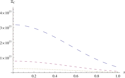
Figure 1: $16\pi^{6}\left[a\left(\tau\right)/H\right]^{2}\Xi_{c}^{\Phi}\left(\tau,\bar{\xi}\right)$ as a function of $\xi$, for fixed $m/H=10^{-6}$ and $\tau_{0}=0.7\times 10^{-9}$ (large dashing), $\tau_{0}=10^{-9}$ (medium dashing) and $\tau_{0}=1.3\times 10^{-9}$ (tiny dashing)

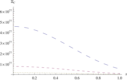
Figure 2: $16\pi^{6}\left[a\left(\tau\right)/H\right]^{2}\Xi_{c}^{\Phi}\left(\tau,\bar{\xi}\right)$ as a function of $\xi$, for fixed $\tau_{0}=10^{-9}$ and $m/H=0.8\times 10^{-6}$ (large dashing), $m/H=10^{-6}$ (medium dashing) and $m/H=1.2\times 10^{-9}$ (tiny dashing)

We can estimate the (dimensionless) coherence length of the kinetic helicity as

$$\Lambda^{2}\left(\frac{m}{H},\tau_{0}\right)\equiv-\left.\frac{\Xi_{c}^{\Phi}\left(\tau,\bar{\xi}\right)}{\partial^{2}\Xi_{c}^{\Phi}\left(\tau,\bar{\xi}\right)/\partial\xi^{2}}\right|_{\xi=0}$$ (51)

In Fig. (3) we show $\Lambda^{2}$ as a function of $m/H$ for $\tau_{0}$ fixed, and in Fig. and (4) the converse. From both figures we see that, for the chosen values of the parameters, $\Lambda\sim 1$, i.e. it is of the order of the particle horizon’s scale.

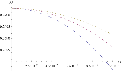
Figure 3: $\Lambda^{2}$ as a function of $\tau_{0}$, and for $m/H=0.8\times 10^{-6}$ (large dashing), $m/H=10^{-8}$ (medium dashing) and $m/H=1.2\times 10^{-9}$ (tiny dashing)

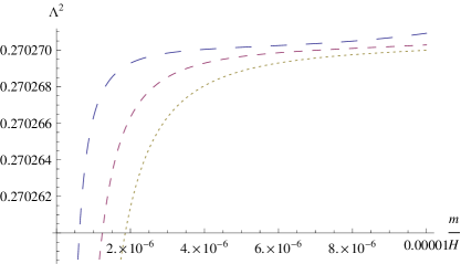
Figure 4: $\Lambda^{2}$ as a function of $m/H$, and for $\tau_{0}=0.7\times 10^{-9}$ (large dashing), $\tau_{0}=10^{-9}$ (medium dashing) and $\tau_{0}=1.3\times 10^{-9}$ (tiny dashing)

The r.m.s. value of the kinetic helicity is obtained by volume averaging expression (50) over $x$ and $x^{\prime}$, i.e.

$$\Sigma_{\mathcal{H}_{c}}^{2}=\frac{1}{Vol\left(x\right)}\int_{Vol\left(x\right)}d\left[vol\left(x\right)\right]\frac{1}{Vol\left(x^{\prime}\right)}\int_{Vol\left(x^{\prime}\right)}d\left[vol\left(x^{\prime}\right)\right]~{}\Xi_{c}^{\Phi}\left(\tau,\bar{x},\bar{x}^{\prime}\right)$$ (52)

Kinetic helicity is a global quantity, that can depend at most on the dimensionless characteristic scale $\mathcal{L}<1$ of the integration volume. To evaluate the integrals in eq. (52) we can proceed as follows. As we are considering scales $\lesssim 1$ we can develop eq. (50) in Taylor series to second order in $\bar{x}-\bar{x}^{\prime}$, then using eq. (35) we have

$$\Sigma_{\mathcal{H}_{c}}\left(\tau,\mathcal{L}\right) \sim\frac{8H\tau_{0}^{4}}{\pi a\left(\tau\right)}\left[\frac{3}{2}\left(\frac{H}{m}\right)^{2}\tau_{0}^{2}+\left(\frac{9}{16}\right)^{4}\frac{1}{24}\right]^{-2}$$

$$\times A^{1/2}\left(\frac{m}{H},\tau_{0}\right)\left[1-\frac{1}{240}\frac{\mathcal{L}^{2}}{\Lambda^{2}\left(m/H,\tau_{0}\right)}\right]^{1/2}$$ (53)

where $\mathcal{L}=HL$, and with

$$A\left(\frac{m}{H},\tau_{0}\right) \simeq-\frac{2187}{2097152}\frac{1}{\tau_{0}^{2}}\left[\frac{3}{8}\left(\frac{H}{m}\right)^{4}+\frac{1}{2}\left(\frac{H}{m}\right)^{2}+\frac{9477}{29360128}\frac{1}{\tau_{0}^{2}}\right]$$

$$\times\left\{\left[\frac{1}{12}\frac{H}{m}-\frac{2187}{5242880}\frac{1}{\tau_{0}^{2}}\right]^{2}-\left[\frac{3}{8}\left(\frac{H}{m}\right)^{2}+\frac{2187}{4194304}\frac{1}{\tau_{0}^{2}}\right]\right.$$

$$\times\left.\left[\frac{3}{8}\left(\frac{H}{m}\right)^{4}+\frac{1}{2}\left(\frac{H}{m}\right)^{2}+\frac{9477}{29360128}\frac{1}{\tau_{0}^{2}}\right]\right\}$$ (54)

the zeroth order in the Taylor expansion of $\Xi_{c}^{\Phi}\left(\tau,\bar{\xi}\right)$.

4 Characterizing the turbulence: viscosity, Reynolds number and characteristic decay and correlation times

Turbulence sets in at the inflation-reheating transition, and afterward, as there is no stirring forces acting on the flow, it decays. Since the fluid is made of particle - antiparticle pairs, annihilation also occurs. We have two competing processes, whose characteristic times must be compared in order to decide which one dominates: the decay time of turbulence and the time of particle anti-particle annihilation.

To properly characterize the turbulence, we must first calculate the Reynolds number of the flow. This number is defined as $Re=ul/\upsilon$, with $u$ and $l$ characteristics velocity and scale respectively and $\upsilon$ the kinematic viscosity. As it may happen that turbulence is not fully developed at all scales, we must calculate this number for each scale. The scale dependent Reynolds number can be written as

$$Re\left(\kappa\right)=\frac{k^{-1}\mathtt{v}_{\kappa}}{\upsilon}$$ (55)

where $\upsilon=\eta/\left\langle\rho+p\right\rangle$ is the dimensionless ratio of the fluid shear viscosity to the energy density $k^{-1}=a\left(\tau\right)H^{-1}\kappa^{-1}$ is the scale of interest and $\mathtt{v}_{\kappa}\sim\sqrt{2E_{\kappa}\left(\tau\right)}$ the estimate of the velocity at the corresponding scale. To estimate $\eta$ we follow the work of Son and collaborators [45], and consider it proportional to the entropy density, i.e., $\eta/s=1/4\pi$. We take $s$ as proportional to the quasiparticle number density $n$, i.e., $s\sim n\left(\tau\right)$, with $n\left(\tau\right)$

$$n\left(\tau\right)\simeq\frac{H^{3}}{a^{3}\left(\tau\right)}\frac{1}{\tau_{0}^{2}}\left[\frac{3}{2}\frac{H^{3}}{m^{3}}\tau_{0}^{2}+\left(\frac{9}{16}\right)^{4}\frac{\pi}{28}\right]$$ (56)

(see Appendix B). Using eq. (35) we have that

$$\upsilon\left(\tau\right)\simeq\frac{1}{\left(2\pi\right)^{1/2}}\frac{a\left(\tau\right)}{H}\frac{\left[\left(3/2\right)\left(H/m\right)^{3}\tau_{0}^{2}+\left(9/16\right)^{4}\pi/28\right]}{\left[\left(3/2\right)\left(H/m\right)^{2}\tau_{0}^{2}+\left(9/16\right)^{4}/24\right]}$$ (57)

Replacing everything into eq. (55) we obtain

$$Re\left(\kappa,\tau\right)\simeq\left(2\pi\right)^{1/2}\left(\frac{9}{16}\right)^{2}\sqrt{\frac{3}{256}}\frac{a^{1/2}\left(\tau\right)\left(H/m\right)^{2}\tau_{0}}{\left[\left(3/2\right)\left(H/m\right)^{3}\tau_{0}^{2}+\left(9/16\right)^{4}\pi/28\right]}\frac{1}{\kappa^{4}}$$ (58)

We see that, for $\kappa\sim 1$, we can have $Re\gg 1$ if

$$\left(2\pi\right)^{1/2}\frac{2}{3}\left(\frac{9}{16}\right)^{2}\sqrt{\frac{3}{256}}\gg\frac{H}{m}\tau_{0}$$ (59)

i.e., if the transition between inflation and reheating is very fast. In Fig. (5) we plot $Re\left(\kappa,\tau\right)/a^{1/2}\left(\tau\right)$ as a function of $\kappa$ for fixed $m/H$ and three values of $\tau_{0}$, it is seen that $Re$ increases as the duration of the transition inflation/reheating shortens. In Fig. (6) we plot the same as in the first figure, but with fixed $\tau_{0}=10^{-9}$ and $m/H=10^{-5}$, $10^{-6}$ and $10^{-7}$, and we observe that $Re$ diminishes with decreasing $m/H$. In both figures $Re$ is a decreasing function of $\kappa$, hence only the modes near the horizon can be considered as turbulent. In Fig. (7) we plot $Re\left(\kappa=1,\tau\right)/a^{1/2}\left(\tau\right)$ as a function of $\tau_{0}$ and for $m/H=10^{-5}$, $10^{-6}$ and $10^{-7}$. In this case $Re$ has a peak at certain value of $\tau_{0}$, and this peak is higher and occurs at shorter values of $\tau_{0}$ as $m/H$ diminishes. As $\tau_{0}$ grows $Re$ decreases monotonically. Finally, in Fig. (8) we show $Re/a^{1/2}\left(\tau\right)$ as a function of $m/H$, for $\kappa=1$ and $\tau_{0}=10^{-7}$, $10^{-8}$ e $10^{-9}$. Again $Re$ peaks at certain values of $m/H$ and the peak is higher and occurs at smaller values of $m/H$ as $\tau_{0}$ diminishes.

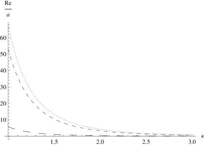
Figure 5: $Re\left(\kappa,\tau\right)/a^{1/2}\left(\tau\right)$ as a function of $\kappa$, for fixed $m/H=10^{-5}$ and $\tau_{0}=10^{-7}$ (large dashing), $10^{-8}$ (medium dashing) and $10^{-9}$ (tiny dashing). $Re$ increases as $\tau_{0}$ diminishes

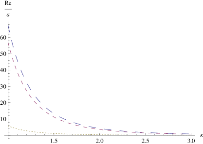
Figure 6: $Re\left(\kappa,\tau\right)/a^{1/2}\left(\tau\right)$ as a function of $\kappa$, for fixed $\tau_{0}=10^{-9}$ and $m/H=10^{-5}$ (large dashing), $10^{-6}$ (medium dashing) and $10^{-7}$ (tiny dashing). $Re$ diminishes as $m/H$ diminishes

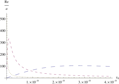
Figure 7: $Re\left(\kappa=1,\tau\right)/a^{1/2}\left(\tau\right)$ as a function of $\tau_{0}$, and for $m/H=10^{-5}$ (large dashing), $10^{-6}$ (medium dashing) and $10^{-7}$ (tiny dashing). Observe that $Re$ peaks at a certain value of $\tau_{0}$. The peak is higher and occurs at smaller values of $\tau_{0}$ as $m/H$ diminishes.

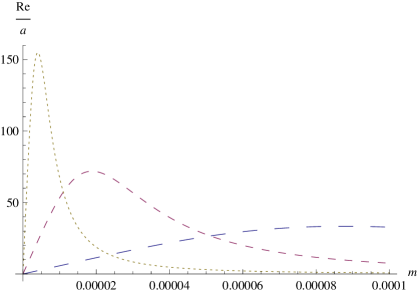
Figure 8: $Re\left(\kappa=1,\tau\right)/a^{1/2}\left(\tau\right)$ as a function of $m/H$, and for $\tau_{0}=10^{-7}$ (large dashing), $10^{-8}$ (medium dashing) and $10^{-9}$ (tiny dashing). Observe that $Re$ again peaks at a certain value of $m/H$. The peak is higher and occurs at smaller values of $m/H$ as $\tau_{0}$ diminishes.

The decay time of each turbulent mode is given by $t_{d}\left(k\right)=1/\upsilon k^{2}=a^{2}\left(\tau\right)H^{-2}/\upsilon\kappa^{2}$. Using eq. (57) we can write

$$t_{d}\left(\kappa\right)\simeq\frac{\left(2\pi\right)^{1/2}a\left(\tau\right)}{H}\frac{\left[\left(3/2\right)\left(H/m\right)^{2}\tau_{0}^{2}+\left(9/16\right)^{4}/24\right]}{\left[\left(3/2\right)\left(H/m\right)^{3}\tau_{0}^{2}+\left(9/16\right)^{4}\pi/28\right]}\frac{1}{\kappa^{2}}$$ (60)

To estimate the pair annihilation time of each mode, we consider that the particles are relativistic, according to the result obtained for their energy density. On a dimensional basis, this time can be estimated as

$$t_{a}\left(\kappa\right)\sim\frac{1}{n\left(\tau\right)\sigma_{\kappa}u_{r}}$$ (61)

with $n\left(\tau\right)$ the particle density, $\sigma_{\kappa}$ the annihilation cross-section and $u_{r}$ the relative velocity between species which we take $u_{r}\sim 1$. We make a crude estimation of the cross section, as being the same as for $e^{+}e^{-}$ annihilation [54] for $\gamma\gg 1$. i.e., $\sigma\simeq\pi r_{0}^{2}/\gamma$, with, $r_{0}=\alpha/m$, $\alpha=1/137$ the fine-structure constant, $\gamma=\varepsilon/m$ with $m$ the particles mass and $\varepsilon\sim H\Omega_{\kappa}=H\left[\kappa^{2}/a^{2}\left(\tau\right)+\left(m/H\right)^{2}\right]^{1/2}$ the maximum energy of each mode. We then have

$$\sigma_{\kappa}\simeq\pi\frac{\alpha^{2}}{mH}\frac{a\left(\tau\right)}{\sqrt{\kappa^{2}+a^{2}\left(\tau\right)\left(m/H\right)^{2}}}$$ (62)

replacing in eq. (61) we have

$$t_{a}\left(\kappa\right)\sim\frac{a^{2}\left(\tau\right)}{\pi\alpha^{2}}\frac{m\tau_{0}^{2}}{H^{2}}\frac{\sqrt{\kappa^{2}+a^{2}\left(\tau\right)\left(m/H\right)^{2}}}{\left[\left(3/2\right)\left(H/m\right)^{3}\tau_{0}^{2}+\left(9/16\right)^{4}/28\right]}$$ (63)

Comparing both times we have

$$\frac{t_{d}\left(\kappa\right)}{t_{a}\left(\kappa\right)}\simeq\frac{\left(2\pi^{3}\right)^{1/2}\alpha^{2}}{a\left(\tau\right)}\frac{H}{m\tau_{0}^{2}}\frac{\left[\left(3/2\right)\left(H/m\right)^{2}\tau_{0}^{2}+\left(9/16\right)^{4}/24\right]}{\kappa^{2}\sqrt{\kappa^{2}+a^{2}\left(\tau\right)\left(m/H\right)^{2}}}$$ (64)

as $H/m\gg 1$ and $\tau_{0}^{2}\ll 1$ we have that $t_{d}\left(\kappa\right)/t_{a}\left(\kappa\right)\gg 1$, i.e., annihilation occurs before the end of turbulence.

It can be seen that $t_{a}$ is also much shorter than other time scales pertaining to the flow, such as the ratio between the radius of the largest turbulent eddy (i.e., the horizon as it is there where $Re\left(\kappa\right)$ takes its largest value) to the velocity associated to that scale. Therefore in what follows we take $t_{corr}\equiv t_{a}$.

5 Magnetic field amplification due to dynamo action

According to eq. (8) we must now evaluate the amplification exponent, $\Sigma{\mathcal{H}_{c}}^{2}\left(\tau,\mathcal{L}\right)t\left(\kappa\right)/\mathtt{L}a\left(\tau\right)$, where $\mathtt{L}a\left(\tau\right)$ is the physical coherence scale of the magnetic field and $\mathcal{L}$ is the (dimensionless) coherent scale of the kinetic helicity. From the discussion in Section III, the shortest time is the annihilation time, which for scales such that $\kappa\sim 1/\mathcal{L}>m/H$ reads

$$t_{a}\left(\mathcal{L}\right)\sim\frac{a^{2}\left(\tau\right)}{\pi\alpha^{2}}\frac{m\tau_{0}^{2}}{H^{2}}\frac{1}{\left[\left(3/2\right)\left(H/m\right)^{3}\tau_{0}^{2}+\left(9/16\right)^{4}/28\right]}\frac{1}{\mathcal{L}}$$ (65)

Writing $\mathtt{L}=H^{-1}\mathfrak{L}$ the amplification exponent reads

$$\frac{\Sigma_{\mathcal{H}_{c}}\left(\tau,\mathcal{L}\right)t_{a}\left(\mathcal{L}\right)}{\mathtt{L}a\left(\tau\right)} \sim \frac{8}{\pi^{3}\alpha^{4}}a^{3}\left(\tau\right)\frac{m^{2}\tau_{0}^{8}}{H^{2}}\frac{1}{\mathfrak{L}\mathcal{L}^{2}}\frac{1}{\left[\left(3/2\right)\left(H/m\right)^{2}\tau_{0}^{2}+\left(9/16\right)^{4}1/24\right]^{2}}$$ (66)

$$\times\frac{1}{\left[\left(3/2\right)\left(H/m\right)^{3}\tau_{0}^{2}+\left(9/16\right)^{4}/28\right]^{2}}$$

$$\times A^{1/2}\left(\frac{m}{H},\tau_{0}\right)\left[1-\frac{1}{240}\frac{\mathcal{L}^{2}}{\Lambda^{2}\left(m/H,\tau_{0}\right)}\right]^{1/2}$$

which by simple inspection is seen to be very small.

6 Discussion and Conclusions

In this paper we have studied the possibility of turbulent dynamo action during reheating. We considered the presence of a charged scalar field minimally coupled to gravity. This field is in its invariant vacuum state during inflation. When the transition to reheating takes place the vacuum state turns into a many-particle state. For sub-horizon modes of the field, the number of created modes depends on the details of the transition. Therefore during reheating, besides the decay products of the inflaton we also have a plasma of scalar particles which is at rest in the comoving frame. We characterize the fluctuating velocities of this plasma giving their spatial two point correlation function and the kinetic energy associated to each Fourier mode of the stochastic velocity field, eq. (44). We evaluate the Reynolds number associated to each mode, $Re\left(\kappa\right)$, which turns out to depend on the physical parameters of the problem, namely $m$, $H$ and the duration $\tau_{0}$ of the transition from inflation to reheating. If $\tau_{0}$ is small enough, then there is a range of $\kappa$ for which $Re\left(\kappa\right)>1$ and the flow can be considered as (mildly) turbulent. As there are no stirring forces, the turbulence we refer to decays, each mode doing so in a characteristic time $t_{d}\left(\kappa\right)$ given by eq. (60). Besides as the plasma is a particle anti-particle one, each mode of the scalar field (not to be confused with modes of the stochastic velocity field) annihilates in a characteristic time $t_{a}\left(\kappa\right)$ given by eq. (63). When comparing both times we find that annihilation dominates over decay, eq. (64) and hence for practical purposes we can consider the turbulence as steady.

The sufficient condition to have a large scale kinematic dynamo is the flow to be endowed with kinetic helicity [35]. The non-trivial result of this paper is that the scalar plasma does possess a non null rms kinetic helicity,eq. (53) From Figs. (3) and (4) we see that, for the parameters for which $Re\left(\kappa\right)>1$, the characteristic scale of the kinetic helicity is of the order of the particle horizon, thus allowing for kinematic dynamo action.

The existence of an rms helicity is due to the presence of the two scalar fields, $\Phi$ and $\Phi^{\dagger}$, as is evident from eq. (49). Moreover, though the helicity may have either sign, in the average the amplification effect dominates. From the simplest model of kinematic dynamo, eq. (7), we compute the amplification factor of an initial seed field, eq. (66), and find that for the physical parameters of the scenario considered, it is very small. In spite of this result, we believe our work shows the need for exploring the impact of nonlinear effects in the early universe. These effects offer the most natural answer to the riddle of the survival of the primordial magnetic field until the epoch of structure formation, in spite of the $1/a^{2}$ damping induced by the Hubble expansion.

Appendix A Bogoliubov coefficients

We assume that during the reheating period the scale factor of the Universe scales as $t^{2/3}$ [49, 50], while for inflation we consider a spatially flat de Sitter universe. For large wavenumbers the Bogoliubov coefficients are sensitive to the details of the transition, while for small wavenumbers the coefficients can be found assuming an instantaneous transition. This dependence on the transition details for subhorizon modes was also recently analyzed by Zaballa and Sasaki [51] in the context of creation of metric perturbations at the end of inflation.

The Klein Gordon equation for a free field in a FRW Universe is

$$\ddot{\psi}_{\kappa}+\left[\frac{\kappa^{2}}{a^{2}}+\left(\frac{m}{H}\right)^{2}-\frac{3}{2}\left(\frac{\ddot{a}}{a}+\frac{\dot{a}^{2}}{2a^{2}}\right)\right]\psi_{\kappa}=0$$ (67)

It is seen that

$$\frac{3}{2}\left(\frac{\ddot{a}}{a}+\frac{\dot{a}^{2}}{2a^{2}}\right)=\frac{1}{a^{3/2}}\frac{d^{2}a^{3/2}}{d\tau^{2}}\equiv\frac{9}{4}f\left(\varkappa\right)$$ (68)

with $x=\left(\tau-\tau_{1}\right)/\tau_{0}$ where $\tau_{0}$ is the time the transition lasts. We assume $\tau_{0}~{}\tau_{1}\ll 1$. In terms of $x$ eq. (68) gives

$$\frac{d^{2}a^{3/2}}{dx^{2}}=\frac{9}{4}\tau_{0}^{2}a^{3/2}f\left(x\right)$$ (69)

which can be integrated giving

$$a^{3/2}\left(x\right)=A+Bx+\frac{9}{4}\tau_{0}^{2}\int_{-x_{1}}^{x}dy\left(x-y\right)f\left(y\right)a^{3/2}\left(y\right)$$ (70)

where $x_{1}=\tau_{1}/\tau_{0}$. The constants of integration are obtained by matching to the inflationary solution at $\tau=0$. We get $A=1+\tau_{0}x_{1}$ and $B=\tau_{0}$, then

$$a^{3/2}\left(x\right)=1+\tau_{0}\left(x_{1}+x\right)+\frac{9}{4}\tau_{0}^{2}\int_{-x_{1}}^{x}dy\left(x-y\right)f\left(y\right)a^{3/2}\left(y\right)\equiv F\left(x\right)+\tau_{0}xG\left(x\right)$$ (71)

with

$$F\left(x\right) =1+\tau_{0}x_{1}-\frac{9}{4}\tau_{0}^{2}\int_{-x_{1}}^{x}dyyf\left(y\right)a^{3/2}\left(y\right)$$ (72)

$$G\left(x\right) =1+\frac{9}{4}\tau_{0}\int_{-x_{1}}^{x}dyf\left(y\right)a^{3/2}\left(y\right)$$ (73)

For $x\geq 1$ we have $f\sim 0$, hence $F$ and $G$ are constants in that $x$ range. We now write K.G. equation (67) as

$$\frac{d^{2}\psi_{\kappa}}{dx^{2}}+\tau_{0}^{2}\Omega_{\kappa}^{2}\left(x\right)\psi_{\kappa}=0$$ (74)

with

$$\Omega_{\kappa}^{2}\left(x\right)=\frac{\kappa^{2}}{a^{2}}+\frac{m^{2}}{H^{2}}-\frac{9}{4}f\left(x\right)$$ (75)

We are interested in the behavior of the solutions equivalent to $H_{\nu}^{\left(1\right)}\left(x\right)$ (the positive frequency solutions for a spatially flat de Sitter spacetime) in $x=-x_{1}$. There are two possible situations. Given that $x=0$ is the middle of the transition, we consider: (a) $\Omega\left(0\right)\tau_{0}<1$: the details of the transition are not important; (b) $\Omega\left(0\right)\tau_{0}>1$: the details of the transition matter. For modes inside the horizon ($\kappa\geq 1$) we can consider the WKB solution

$$\varphi_{\kappa+}\left(x\right)=\frac{e^{i\tau_{0}S\left[x\right]}}{\sqrt{2\Omega_{\kappa}\left(x\right)}}$$ (76)

with $\Omega\left(x\right)=dS\left[x\right]/dx$. The derivatives are

$$\frac{d\varphi_{\kappa+}}{dx}=-\left[i\tau_{0}\Omega_{\kappa}\left(x\right)+\frac{1}{2}\frac{\Omega_{\kappa}^{\prime}\left(x\right)}{\Omega_{\kappa}\left(x\right)}\right]\varphi_{\kappa+}$$ (77)

$$\frac{d^{2}\varphi_{\kappa+}}{dx^{2}}=-\left[\tau_{0}^{2}\Omega_{\kappa}^{2}\left(x\right)-\frac{1}{4}\left(\frac{\Omega_{\kappa}^{\prime}\left(x\right)}{\Omega_{\kappa}\left(x\right)}\right)^{2}+\frac{1}{2}\left(\frac{\Omega_{\kappa}^{\prime}\left(x\right)}{\Omega_{\kappa}\left(x\right)}\right)^{\prime}\right]\varphi_{\kappa+}$$ (78)

and then the equation for $\psi_{\kappa}$ reads

$$\frac{d^{2}\psi_{\kappa}}{dx^{2}}+ \left[\tau_{0}^{2}\Omega_{\kappa}^{2}\left(x\right)-\frac{1}{4}\left(\frac{\Omega_{\kappa}^{\prime}\left(x\right)}{\Omega_{\kappa}\left(x\right)}\right)^{2}+\frac{1}{2}\left(\frac{\Omega_{\kappa}^{\prime}\left(x\right)}{\Omega_{\kappa}\left(x\right)}\right)^{\prime}\right]\psi_{\kappa}$$

$$=\left[-\frac{1}{4}\left(\frac{\Omega_{\kappa}^{\prime}\left(x\right)}{\Omega_{\kappa}\left(x\right)}\right)^{2}+\frac{1}{2}\left(\frac{\Omega_{\kappa}^{\prime}\left(x\right)}{\Omega_{\kappa}\left(x\right)}\right)^{\prime}\right]\psi_{\kappa}$$ (79)

The solution can be expressed as a superposition of positive and negative frequency modes as

$$\psi_{\kappa}\left(x\right) =\varphi_{\kappa+}\left(x\right)+\frac{i}{\tau_{0}}\varphi_{\kappa+}\left(x\right)\int_{-x_{1}}^{x_{1}}dy\varphi_{\kappa-}\left(y\right)\left[-\frac{1}{4}\left(\frac{\Omega_{\kappa}^{\prime}}{\Omega_{\kappa}}\right)^{2}+\frac{1}{2}\left(\frac{\Omega_{\kappa}^{\prime}}{\Omega_{\kappa}}\right)^{\prime}\right]\psi_{\kappa}\left(y\right)$$

$$-\frac{i}{\tau_{0}}\varphi_{\kappa-}\left(x\right)\int_{-x_{1}}^{x_{1}}dy\varphi_{\kappa+}\left(y\right)\left[-\frac{1}{4}\left(\frac{\Omega_{\kappa}^{\prime}}{\Omega_{\kappa}}\right)^{2}+\frac{1}{2}\left(\frac{\Omega_{\kappa}^{\prime}}{\Omega_{\kappa}}\right)^{\prime}\right]\psi_{\kappa}\left(y\right)$$ (80)

Whereby we read the Bogoliubov coefficients

$$\alpha_{\kappa}=1+\frac{i}{\tau_{0}}\int_{-x_{1}}^{x_{1}}dy\varphi_{\kappa-}\left(y\right)\left[-\frac{1}{4}\left(\frac{\Omega_{\kappa}^{\prime}}{\Omega_{\kappa}}\right)^{2}+\frac{1}{2}\left(\frac{\Omega_{\kappa}^{\prime}}{\Omega_{\kappa}}\right)^{\prime}\right]\psi_{\kappa}\left(y\right)$$ (81)

$$\beta_{\kappa}=-\frac{i}{\tau_{0}}\int_{-x_{1}}^{x_{1}}dy\varphi_{\kappa+}\left(y\right)\left[-\frac{1}{4}\left(\frac{\Omega_{\kappa}^{\prime}}{\Omega_{\kappa}}\right)^{2}+\frac{1}{2}\left(\frac{\Omega_{\kappa}^{\prime}}{\Omega_{\kappa}}\right)^{\prime}\right]\psi_{\kappa}\left(y\right)$$ (82)

which should satisfy $\left|\alpha_{\kappa}\right|^{2}-\left|\beta_{\kappa}\right|^{2}=1$. To obtain a simpler expression, we consider an iterative solution. To lowest order, i.e., $\psi\left(y\right)\simeq\varphi_{+}\left(y\right)$, we have

$$\alpha_{\kappa}^{\left(0\right)}=1+\frac{i}{\tau_{0}}\int_{-x_{1}}^{x_{1}}dy\varphi_{\kappa-}\left(y\right)\varphi_{\kappa+}\left(y\right)\left[-\frac{1}{4}\left(\frac{\Omega_{\kappa}^{\prime}}{\Omega_{\kappa}}\right)^{2}+\frac{1}{2}\left(\frac{\Omega_{\kappa}^{\prime}}{\Omega_{\kappa}}\right)^{\prime}\right]$$ (83)

$$\beta_{\kappa}^{\left(0\right)}\simeq-\frac{i}{\tau_{0}}\int_{-x_{1}}^{x_{1}}dy\varphi_{\kappa+}^{2}\left(y\right)\left[-\frac{1}{4}\left(\frac{\Omega_{\kappa}^{\prime}}{\Omega_{\kappa}}\right)^{2}+\frac{1}{2}\left(\frac{\Omega_{\kappa}^{\prime}}{\Omega_{\kappa}}\right)^{\prime}\right]$$ (84)

and

$$\psi_{\kappa}\left(x\right)=\alpha_{\kappa}^{\left(0\right)}\varphi_{\kappa+}\left(x\right)+\beta_{\kappa}^{\left(0\right)}\varphi_{\kappa-}\left(x\right)$$ (85)

Performing another iteration we obtain

$$\alpha_{\kappa}^{\left(1\right)}\simeq\exp\left[\frac{i}{\tau_{0}}\int_{-x_{1}}^{x_{1}}dy\varphi_{\kappa+}\left(y\right)\varphi_{\kappa-}\left(y\right)Q_{\kappa}\left(y\right)\right]\left(1+\frac{1}{2}\left|\beta_{\kappa}^{\left(0\right)}\right|^{2}\right)$$ (86)

Observe that it is not necessary to perform another iteration for $\beta_{k}$. The normalization condition $\left|\alpha_{\kappa}\right|^{2}-\left|\beta_{\kappa}\right|^{2}=1$ is satisfied up to a term $\left|\beta_{\kappa}^{\left(0\right)}\right|^{4}/4$, indicating that this coefficient must be $\left|\beta_{\kappa}^{\left(0\right)}\right|^{2}\ll 1$ in order to render our expressions valid.

Integrating by parts in eq eq. (82) and neglecting surface terms we have

$$\int_{-x_{1}}^{x_{1}}dy\varphi_{\kappa+}^{2}\left(y\right)\frac{1}{2}\left(\frac{\Omega_{\kappa}^{\prime}}{\Omega_{\kappa}}\right)^{\prime} =-\int_{-x_{1}}^{x_{1}}dy\frac{\Omega_{\kappa}^{\prime}}{\Omega_{\kappa}}\varphi_{\kappa+}\left(y\right)\varphi_{\kappa+}^{\prime}\left(y\right)$$ (87)

$$=-\int_{-x_{1}}^{x_{1}}dy\frac{\Omega_{\kappa}^{\prime}}{\Omega_{\kappa}}\varphi_{\kappa+}^{2}\left(y\right)\left[-i\tau_{0}\Omega_{\kappa}-\frac{1}{2}\frac{\Omega_{\kappa}^{\prime}}{\Omega_{\kappa}}\right]$$

Observe that the first term is suppressed by a factor of $\tau_{0}$, so we shall not consider it further. We are now at the point where details begin to matter. Write

$$\frac{\Omega_{\kappa}^{\prime}}{\Omega_{\kappa}}=\frac{1}{2\Omega_{\kappa}^{2}}\left[\frac{-2\kappa^{2}}{a^{2}}\frac{a^{\prime}}{a}-\frac{9}{4}f^{\prime}\left(x\right)\right]$$ (88)

The $\kappa^{2}$ term may be neglected even when $\kappa^{2}$ is large. To see this, observe that

$$\frac{\kappa^{2}}{a^{2}}=\Omega_{\kappa}^{2}-\left(\frac{m}{H}\right)^{2}+\frac{9}{4}f\left(x\right)$$ (89)

so

$$\frac{\Omega_{\kappa}^{\prime}}{\Omega_{\kappa}}=-\left(\frac{a^{\prime}}{a}\right)-\frac{1}{2\Omega_{\kappa}^{2}}\left[2\left(\frac{9}{4}f\left(x\right)-\left(\frac{m}{H}\right)^{2}\right)\frac{a^{\prime}}{a}+\frac{9}{4}f^{\prime}\left(x\right)\right]$$ (90)

Writing

$$\frac{a^{\prime}}{a}=\frac{2}{3}\frac{\left(a^{3/2}\right)^{\prime}}{a^{3/2}}=\frac{2}{3}\frac{\tau_{0}G\left(x\right)}{\left(F\left(x\right)+\tau_{0}xG\left(x\right)\right)}$$ (91)

we see that this function is suppressed by $\tau_{0}$. Therefore in eq. (90) the only term that is not suppressed is the last one. So we finally have

$$\beta_{\kappa}^{\left(0\right)}\sim-\frac{i}{\tau_{0}}\left(\frac{9}{16}\right)^{2}\int_{-x_{1}}^{x_{1}}dy\left[\frac{f^{\prime}\left(y\right)}{\Omega_{\kappa}^{2}\left(y\right)}\right]^{2}\varphi_{\kappa+}^{2}\left(y\right)$$ (92)

We see that $\beta_{\kappa}$ is essentially the Fourier transform of $\left(f^{\prime}\right)^{2}$. Since this function has a peak whose width is $\sim 1$, by Heisenberg’s principle we expect to get a negligible result for $\tau_{0}\Omega_{\kappa}\gg 1$, namely for $\kappa\gg\tau_{0}^{-1}$. Observe however that this scale can be extremely high. To give concrete results, let us consider $f^{\prime}=const=-1/2$ and assume that we can make a linear approximation in the exponent of eq. (76), $S\left[x\right]\sim S\left[0\right]+\Omega\left[0\right]x$. Assuming $x_{1}\simeq 1$ and that $\Omega_{\kappa}\left(y\right)$ is a slowly varying function of time to keep only the surface terms in the integral, we obtain eq. (26). We see that the number of created particles with large $\kappa$ is very sensitive to the details of the transition between inflation and reheating; it would actually diverge in the limit $\tau_{0}\mapsto 0$, which is therefore unphysical.

For small $\kappa$ an instantaneous transition can be considered, and the coefficients calculated by directly matching the inflationary and reheating solutions at $\tau=0$. Assuming again a WKB form for the modes during reheating and the usual Hankel function for de Sitter [38]. For this transition the full expression for $\beta_{\kappa}$ is

$$\beta_{\kappa}=-\frac{\pi^{1/2}}{8^{1/2}\Omega_{\kappa}^{1/2}\left(0\right)}\left\{\kappa H_{\nu-1}^{\left(1\right)}\left(\kappa\right)+H_{\nu}^{\left(1\right)}\left(\kappa\right)\left[\frac{2}{3}\frac{\kappa^{2}}{\Omega_{\kappa}^{2}\left(0\right)}-\nu-i\Omega_{\kappa}\left(0\right)\right]\right\}$$ (93)

with $\nu=\sqrt{9/4-m^{2}/H^{2}}\simeq 3/2-m^{2}/3H^{2}$. For $\kappa<1$ the Hankel functions can be approximated as

$$H_{\nu}^{\left(1\right)}\left(\kappa\right)\simeq-\frac{i}{\pi}\Gamma\left(\nu\right)\left(\frac{\kappa}{2}\right)^{-\nu}$$ (94)

Using $\left(\nu-1\right)\Gamma\left(\nu-1\right)=\Gamma\left(\nu\right)$ and the fact that $2\kappa^{2}/\Omega_{\kappa}^{2}\left(0\right)3-\nu\sim 1$ we get eq. (28)

Appendix B Calculation of $\left\langle\rho+p\right\rangle$ and $n$

In terms of the scalar field we have

$$\left\langle\rho+p\right\rangle\approx\frac{4\left\langle T_{\Phi}^{00}\right\rangle+\left\langle T_{\Phi a}^{a}\right\rangle}{3}$$ (95)

Using eq. (13) we obtain

$$4\left\langle T_{\Phi}^{00}\right\rangle+\left\langle T_{\Phi a}^{a}\right\rangle=H^{4}\left[3\left\langle\dot{\Phi}\dot{\Phi}^{\dagger}\right\rangle+\frac{1}{a^{2}}\left\langle\bar{\nabla}\Phi\cdot\bar{\nabla}\Phi^{\dagger}\right\rangle\right]$$ (96)

Replacing the decompositions (20) and using

$$\left[a_{\kappa},a_{\varpi}^{\dagger}\right]=\left(2\pi\right)^{3/2}a^{3}\left(\tau\right)\delta\left(\bar{\kappa}-\bar{\varpi}\right)$$ (97)

we obtain

$$3\left\langle\dot{\Phi}\dot{\Phi}^{\dagger}\right\rangle+\frac{1}{a^{2}}\left\langle\bar{\nabla}\Phi\cdot\bar{\nabla}\Phi^{\dagger}\right\rangle = \frac{1}{\left(2\pi\right)^{3/2}a^{3}\left(\tau\right)}\int d\bar{\kappa}\left\{3\dot{\phi}_{\kappa}^{I}\left(\tau\right)\dot{\phi}_{\kappa}^{I\ast}\left(\tau\right)\right.$$

$$- 9\frac{\dot{a}\left(\tau\right)}{a\left(\tau\right)}\left[\dot{\phi}_{\kappa}^{I}\left(\tau\right)\phi_{\kappa}^{I\ast}\left(\tau\right)+\phi_{\kappa}^{I}\left(\tau\right)\dot{\phi}_{\kappa}^{I\ast}\left(\tau\right)\right]$$

$$+ \left.\left[27\frac{\dot{a}^{2}\left(\tau\right)}{a^{2}\left(\tau\right)}+\frac{\kappa^{2}}{a^{2}\left(\tau\right)}\right]\phi_{\kappa}^{I}\left(\tau\right)\phi_{\kappa}^{I\ast}\left(\tau\right)\right\}$$

Using decomposition (25) we identify two different contributions to the integrand: one from pure vacuum

$$M_{0} = 3\dot{\phi}_{k}^{R}\left(\tau\right)\dot{\phi}_{k}^{R\ast}\left(\tau\right)-9\frac{\dot{a}\left(\tau\right)}{a\left(\tau\right)}\left[\dot{\phi}_{k}^{R}\left(\tau\right)\phi_{k}^{R\ast}\left(\tau\right)+\phi_{k}^{R}\left(\tau\right)\dot{\phi}_{k}^{R\ast}\left(\tau\right)\right]$$ (99)

$$+ 27\frac{\dot{a}^{2}\left(\tau\right)}{a^{2}\left(\tau\right)}\phi_{k}^{R}\left(\tau\right)\phi_{k}^{R\ast}\left(\tau\right)+\frac{\kappa^{2}}{a^{2}\left(\tau\right)}\phi_{k}^{R}\left(\tau\right)\phi_{k}^{R\ast}\left(\tau\right)$$

and one from the created particles,

$$M_{1} =3\left[\alpha_{k}\beta_{k}^{\ast}\dot{\phi}_{k}^{R}\left(\tau\right)\dot{\phi}_{k}^{R}\left(\tau\right)+\alpha_{k}^{\ast}\beta_{k}\dot{\phi}_{k}^{R\ast}\left(\tau\right)\dot{\phi}_{k}^{R\ast}\left(\tau\right)\right]$$

$$-18\frac{\dot{a}\left(\tau\right)}{a\left(\tau\right)}\left[\alpha_{k}\beta_{k}^{\ast}\phi_{k}^{R}\left(\tau\right)\dot{\phi}_{k}^{R}\left(\tau\right)+\alpha_{\kappa}^{\ast}\beta_{\kappa}\dot{\phi}_{k}^{R\ast}\left(\tau\right)\phi_{k}^{R\ast}\left(\tau\right)\right]$$

$$+\left(27\frac{\dot{a}^{2}\left(\tau\right)}{a^{2}\left(\tau\right)}+\frac{\kappa^{2}}{a^{2}\left(\tau\right)}\right)\left[\alpha_{k}\beta_{k}^{\ast}\phi_{k}^{R2}\left(\tau\right)+\alpha_{k}^{\ast}\beta_{k}\phi_{k}^{R\ast 2}\left(\tau\right)\right]$$ (100)

$$+2\left|\beta_{k}\right|^{2}\left[3\dot{\phi}_{k}^{R\ast}\left(\tau\right)\dot{\phi}_{k}^{R}\left(\tau\right)-9\frac{\dot{a}\left(\tau\right)}{a\left(\tau\right)}\left(\dot{\phi}_{k}^{R}\left(\tau\right)\phi_{k}^{R\ast}\left(\tau\right)+\dot{\phi}_{k}^{R\ast}\left(\tau\right)\phi_{k}^{R}\left(\tau\right)\right)\right.$$

$$+\left.\left(27\frac{\dot{a}^{2}\left(\tau\right)}{a^{2}\left(\tau\right)}+\frac{\kappa^{2}}{a^{2}\left(\tau\right)}\right)\phi_{k}^{R\ast}\left(\tau\right)\phi_{k}^{R}\left(\tau\right)\right]$$

We are interested in $M_{1}$ and of it, the contribution from the $\left|\beta_{k}\right|^{2}$ terms is the most important: as $\alpha_{k}$ oscillates (see eq, [86]), the terms proportional to $\alpha_{k}$ and $\alpha_{k}^{\ast}$ will give negligible contributions when integrated. Replacing the WKB form for $\phi_{k}^{R}\left(\tau\right)$, eq. (24) we obtain

$$3\left\langle\dot{\Phi}\dot{\Phi}^{\dagger}\right\rangle+\frac{1}{a^{2}}\left\langle\bar{\nabla}\Phi\cdot\bar{\nabla}\Phi^{\dagger}\right\rangle =\frac{1}{\left(2\pi\right)^{3/2}a^{3}\left(\tau\right)}\int d\bar{\kappa}\left|\beta_{k}\right|^{2}\left\{3\left[\Omega_{k}\left(\tau\right)+\frac{1}{4}\frac{\dot{\Omega}_{k}^{2}\left(\tau\right)}{\Omega_{k}^{3}\left(\tau\right)}\right]\right.$$

$$+\left.\frac{9}{2}\frac{\dot{a}\left(\tau\right)}{a\left(\tau\right)}\frac{\dot{\Omega}_{k}\left(\tau\right)}{\Omega_{k}^{2}\left(\tau\right)}+\left[27\frac{\dot{a}^{2}\left(\tau\right)}{a^{2}\left(\tau\right)}+\frac{\kappa^{2}}{a^{2}\left(\tau\right)}\right]\frac{1}{\Omega_{k}\left(\tau\right)}\right\}$$ (101)

Replacing

$$\frac{\dot{a}}{a} =\frac{1}{a^{3/2}},$$

$$\dot{\Omega}_{\kappa}\left(\tau\right) =-\frac{1}{a^{7/2}}\frac{\kappa^{2}}{\Omega_{\kappa}\left(\tau\right)},$$

$$\frac{\dot{\Omega}_{k}\left(\tau\right)}{\Omega_{k}^{2}\left(\tau\right)} =-\frac{1}{a^{7/2}}\frac{\kappa^{2}}{\Omega_{\kappa}^{3}\left(\tau\right)},$$

$$\frac{\dot{\Omega}_{k}^{2}\left(\tau\right)}{\Omega_{k}^{3}\left(\tau\right)} =\frac{1}{a^{7}}\frac{\kappa^{4}}{\Omega_{\kappa}^{5}\left(\tau\right)}$$ (102)

we have that

$$3\left\langle\dot{\Phi}\dot{\Phi}^{\dagger}\right\rangle+ \frac{1}{a^{2}}\left\langle\bar{\nabla}\Phi\cdot\bar{\nabla}\Phi^{\dagger}\right\rangle\rightarrow$$

$$\rightarrow\frac{1}{\left(2\pi\right)^{3/2}a^{3}\left(\tau\right)}\int d\bar{\kappa}\left|\beta_{k}\right|^{2}\left\{3\left[\Omega_{k}\left(\tau\right)+\frac{1}{4}\frac{\kappa^{4}}{a^{7}\left(\tau\right)\Omega_{\kappa}^{5}\left(\tau\right)}\right]\right.$$

$$-\left.\frac{9}{2}\frac{\kappa^{2}}{a^{5}\left(\tau\right)\Omega_{\kappa}^{3}\left(\tau\right)}+\left[\frac{27}{a^{3}\left(\tau\right)}+\frac{\kappa^{2}}{a^{2}\left(\tau\right)}\right]\frac{1}{\Omega_{k}\left(\tau\right)}\right\}$$ (103)

By simple inspection we can see that the terms that contribute the most are

$$3\left\langle\dot{\Phi}\dot{\Phi}^{\dagger}\right\rangle +\frac{1}{a^{2}}\left\langle\bar{\nabla}\Phi\cdot\bar{\nabla}\Phi^{\dagger}\right\rangle\simeq$$

$$\simeq\frac{1}{\left(2\pi\right)^{3/2}a^{3}\left(\tau\right)}\int d\bar{\kappa}\left|\beta_{k}\right|^{2}\left[3\Omega_{k}\left(\tau\right)+\frac{\kappa^{2}}{a^{2}\left(\tau\right)}\frac{1}{\Omega_{k}\left(\tau\right)}\right]$$ (104)

because they decay more slowly than the others. We must now replace the Bogoliubov coefficients and perform the integrations. For long wavelengths, i.e., those in the the interval $\left(0,1\right)$ we use the expression (28). Thus in this case we must evaluate

$$3\left\langle\dot{\Phi}\dot{\Phi}^{\dagger}\right\rangle +\left.\frac{1}{a^{2}}\left\langle\bar{\nabla}\Phi\cdot\bar{\nabla}\Phi^{\dagger}\right\rangle\right|_{\left(0\right)}$$

$$\simeq\frac{\left(\nu-1\right)^{2}\Gamma^{2}\left(1/2\right)}{\left(2\pi\right)^{3/2}\pi a^{3}\left(\tau\right)}\int_{0}^{1}\frac{d\bar{\kappa}}{\Omega_{\kappa}\left(0\right)}\frac{1}{\kappa^{2\nu}}\left[3\Omega_{k}\left(\tau\right)+\frac{\kappa^{2}}{a^{2}\left(\tau\right)}\frac{1}{\Omega_{k}\left(\tau\right)}\right]$$ (105)

Since $m/H\ll 1$ and we are considering a period of time in which $a\left(\tau\right)$ does not differ very much from unity, we can take $a\left(\tau\right)\simeq 1$ in all the roots, and so we have

$$\left.3\left\langle\dot{\Phi}\dot{\Phi}^{\dagger}\right\rangle+\frac{1}{a^{2}}\left\langle\bar{\nabla}\Phi\cdot\bar{\nabla}\Phi^{\dagger}\right\rangle\right|_{\left(0\right)} \simeq\frac{1}{2\left(2\pi\right)^{1/2}a^{4}\left(\tau\right)}$$

$$\times\int_{0}^{1}d\kappa\left[\frac{3}{\kappa^{2\nu-2}}+\frac{\kappa^{4-2\nu}}{\left(\kappa^{2}+m^{2}/H^{2}\right)}\right]$$ (106)

And finally the contribution from long wavelengths reads

$$\left.3\left\langle\dot{\Phi}\dot{\Phi}^{\dagger}\right\rangle+\frac{1}{a^{2}}\left\langle\bar{\nabla}\Phi\cdot\bar{\nabla}\Phi^{\dagger}\right\rangle\right|_{\left(0\right)}\simeq\frac{1}{\left(2\pi\right)^{1/2}a^{4}\left(\tau\right)}\frac{3}{4}\left(\frac{H}{m}\right)^{2}$$ (107)

To evaluate the contribution from the short wavelengths we use eq. (27) in eq. (104), so we have to compute

$$3\left\langle\dot{\Phi}\dot{\Phi}^{\dagger}\right\rangle+ \left.\frac{1}{a^{2}}\left\langle\bar{\nabla}\Phi\cdot\bar{\nabla}\Phi^{\dagger}\right\rangle\right|_{\left(\infty\right)}\simeq\left(\frac{9}{16}\right)^{4}\frac{1}{16}\frac{1}{\tau_{0}^{4}}\frac{2}{\left(2\pi\right)^{1/2}a^{4}\left(\tau\right)}$$ (108)

$$\times\int_{1}^{\infty}d\kappa\frac{1}{\kappa^{8}}\left[3\left(\kappa^{2}+a^{2}\left(\tau\right)m^{2}/H^{2}\right)^{1/2}+\frac{\kappa^{2}}{\left(\kappa^{2}+a^{2}\left(\tau\right)m^{2}/H^{2}\right)^{1/2}}\right]$$

As in this case $m/H\ll\kappa$, we can neglect that term and so the contribution from short wavelengths reads

$$\left.3\left\langle\dot{\Phi}\dot{\Phi}^{\dagger}\right\rangle+\frac{1}{a^{2}}\left\langle\bar{\nabla}\Phi\cdot\bar{\nabla}\Phi^{\dagger}\right\rangle\right|_{\left(\infty\right)}\simeq\left(\frac{9}{16}\right)^{4}\frac{1}{24}\frac{1}{\tau_{0}^{2}}\frac{\pi}{\left(2\pi\right)^{3/2}a^{4}\left(\tau\right)}$$ (109)

Gathering expressions (107) and (109), approximating $\nu-1\simeq 1/2$ and using that $\Gamma\left(1/2\right)=\pi^{1/2}$ we arrive at expression (35).

For $n$, the number density of created particles, we have [38, 39, 40]

$$n=\frac{H^{3}}{a^{3}\left(\tau\right)}\int_{0}^{\infty}d\bar{\kappa}\left|\beta_{\kappa}\right|^{2}$$ (110)

Using again eqs. (28) and (27) in the appropriate momentum intervals we obtain eq. (56).

Appendix C Calculation of the velocity correlation spectrum

We start by replacing eq. (33) into (32) and noting that three kernels build the correlation function: one with the vacuum contributions

$$N_{\left(00\right)}^{ij}\left(\kappa,\varpi,\tau,\tau^{\prime}\right) =\varpi^{i}\kappa^{j}\frac{\partial}{\partial\tau}G_{\kappa}^{R+}\left(\tau,\tau^{\prime}\right)\frac{\partial}{\partial\tau^{\prime}}G_{\varpi}^{R+}\left(\tau,\tau^{\prime}\right)$$

$$+\kappa^{i}\varpi^{j}\frac{\partial}{\partial\tau}G_{\varpi}^{R+}\left(\tau,\tau^{\prime}\right)\frac{\partial}{\partial\tau^{\prime}}G_{\kappa}^{R+}\left(\tau,\tau^{\prime}\right)$$ (111)

$$+\varpi^{i}\varpi^{j}\left[\frac{\partial^{2}}{\partial\tau^{\prime}\partial\tau}G_{\kappa}^{R+}\left(\tau,\tau^{\prime}\right)\right]G_{\varpi}^{R+}\left(\tau,\tau^{\prime}\right)$$

$$+\kappa^{i}\kappa^{j}\left[\frac{\partial^{2}}{\partial\tau^{\prime}\partial\tau}G_{\varpi}^{R+}\left(\tau,\tau^{\prime}\right)\right]G_{\kappa}^{R+}\left(\tau,\tau^{\prime}\right)$$

another with mixed contributions from the vacuum and the created particles,

$$N_{\left(01\right)}^{ij}\left(\kappa,\varpi,\tau,\tau^{\prime}\right)=\varpi^{i}\kappa^{j}\left|\beta_{\kappa}\right|^{2}\left[\frac{\partial}{\partial\tau}G_{\kappa}^{R+}\left(\tau,\tau^{\prime}\right)+\frac{\partial}{\partial\tau}G_{\kappa}^{R-}\left(\tau,\tau^{\prime}\right)\right]\frac{\partial}{\partial\tau^{\prime}}G_{\varpi}^{R+}\left(\tau,\tau^{\prime}\right)$$

$$+\varpi^{i}\kappa^{j}\left|\beta_{\varpi}\right|^{2}\frac{\partial}{\partial\tau}G_{\kappa}^{R+}\left(\tau,\tau^{\prime}\right)\left[\frac{\partial}{\partial\tau^{\prime}}G_{\varpi}^{R+}\left(\tau,\tau^{\prime}\right)+\frac{\partial}{\partial\tau^{\prime}}G_{\varpi}^{R-}\left(\tau,\tau^{\prime}\right)\right]$$ (112)

$$+\varpi^{i}\varpi^{j}\left|\beta_{\kappa}\right|^{2}\left[\frac{\partial^{2}}{\partial\tau^{\prime}\partial\tau}G_{\kappa}^{R+}\left(\tau,\tau^{\prime}\right)+\frac{\partial^{2}}{\partial\tau^{\prime}\partial\tau}G_{\kappa}^{R-}\left(\tau,\tau^{\prime}\right)\right]G_{\varpi}^{R+}\left(\tau,\tau^{\prime}\right)$$

$$+\varpi^{i}\varpi^{j}\left|\beta_{\varpi}\right|^{2}\left[\frac{\partial^{2}}{\partial\tau^{\prime}\partial\tau}G_{\kappa}^{R+}\left(\tau,\tau^{\prime}\right)\right]\left[G_{\varpi}^{R+}\left(\tau,\tau^{\prime}\right)+G_{\varpi}^{R-}\left(\tau,\tau^{\prime}\right)\right]$$

$$+\varpi^{i}\kappa^{j}\alpha_{\varpi}\beta_{\varpi}^{\ast}\frac{\partial}{\partial\tau}G_{\kappa}^{R+}\left(\tau,\tau^{\prime}\right)g_{\varpi}\left(\tau\right)\frac{\partial}{\partial\tau^{\prime}}g_{\varpi}\left(\tau^{\prime}\right)+\varpi^{i}\kappa^{j}\alpha_{\varpi}^{\ast}\beta_{\varpi}\frac{\partial}{\partial\tau}G_{\kappa}^{R+}\left(\tau,\tau^{\prime}\right)g_{\varpi}^{\ast}\left(\tau\right)\frac{\partial}{\partial\tau^{\prime}}g_{\varpi}^{\ast}\left(\tau^{\prime}\right)$$

$$+\varpi^{i}\kappa^{j}\alpha_{\kappa}\beta_{\kappa}^{\ast}\frac{\partial}{\partial\tau}g_{\kappa}\left(\tau\right)g_{\kappa}\left(\tau^{\prime}\right)\frac{\partial}{\partial\tau^{\prime}}G_{\varpi}^{R+}\left(\tau,\tau^{\prime}\right)+\varpi^{i}\kappa^{j}\alpha_{\kappa}^{\ast}\beta_{\kappa}\frac{\partial}{\partial\tau}g_{\kappa}^{\ast}\left(\tau\right)g_{\kappa}^{\ast}\left(\tau^{\prime}\right)\frac{\partial}{\partial\tau^{\prime}}G_{\varpi}^{R+}\left(\tau,\tau^{\prime}\right)$$

$$+\varpi^{i}\varpi^{j}\alpha_{\kappa}\beta_{\kappa}^{\ast}\left[\frac{\partial^{2}}{\partial\tau^{\prime}\partial\tau}g_{\kappa}\left(\tau\right)g_{\kappa}\left(\tau^{\prime}\right)\right]G_{\varpi}^{R+}\left(\tau,\tau^{\prime}\right)+\varpi^{i}\varpi^{j}\alpha_{\varpi}^{\ast}\beta_{\varpi}\left[\frac{\partial^{2}}{\partial\tau^{\prime}\partial\tau}G_{\kappa}^{R+}\left(\tau,\tau^{\prime}\right)\right]g_{\varpi}^{\ast}\left(\tau\right)g_{\varpi}^{\ast}\left(\tau^{\prime}\right)$$

$$+\varpi^{i}\varpi^{j}\alpha_{\kappa}^{\ast}\beta_{\kappa}\left[\frac{\partial^{2}}{\partial\tau^{\prime}\partial\tau}g_{\kappa}^{\ast}\left(\tau\right)g_{\kappa}^{\ast}\left(\tau^{\prime}\right)\right]G_{\varpi}^{R+}\left(\tau,\tau^{\prime}\right)+\varpi^{i}\varpi^{j}\alpha_{\varpi}\beta_{\varpi}^{\ast}\left[\frac{\partial^{2}}{\partial\tau^{\prime}\partial\tau}G_{\kappa}^{R+}\left(\tau,\tau^{\prime}\right)\right]g_{\varpi}\left(\tau\right)g_{\varpi}\left(\tau^{\prime}\right)$$

$$+\left(\varpi\leftrightarrow\kappa\right),$$

and a third kernel with contributions from the created particles,

$$N_{\left(11\right)}^{ij}\left(\kappa,\varpi,\tau,\tau^{\prime}\right) =\varpi^{i}\kappa^{j}\left|\beta_{\kappa}\right|^{2}\left|\beta_{\varpi}\right|^{2}\left(\frac{\partial}{\partial\tau}G_{\kappa}^{R+}\left(\tau,\tau^{\prime}\right)+\frac{\partial}{\partial\tau}G_{\kappa}^{R-}\left(\tau,\tau^{\prime}\right)\right)$$

$$\times\left(\frac{\partial}{\partial\tau^{\prime}}G_{\varpi}^{R+}\left(\tau,\tau^{\prime}\right)+\frac{\partial}{\partial\tau^{\prime}}G_{\varpi}^{R-}\left(\tau,\tau^{\prime}\right)\right)$$

$$+\varpi^{i}\varpi^{j}\alpha_{\kappa}\beta_{\kappa}^{\ast}\left|\beta_{\varpi}\right|^{2}\left(\frac{\partial^{2}}{\partial\tau^{\prime}\partial\tau}g_{\kappa}\left(\tau\right)g_{\kappa}\left(\tau^{\prime}\right)\right)$$

$$\times\left(G_{\varpi}^{R+}\left(\tau,\tau^{\prime}\right)+G_{\varpi}^{R-}\left(\tau,\tau^{\prime}\right)\right)$$

$$+\varpi^{i}\kappa^{j}\left[\alpha_{\kappa}\beta_{\kappa}^{\ast}\alpha_{\varpi}\beta_{\varpi}^{\ast}\frac{\partial}{\partial\tau}g_{\kappa}\left(\tau\right)g_{\kappa}\left(\tau^{\prime}\right)g_{\varpi}\left(\tau\right)\frac{\partial}{\partial\tau^{\prime}}g_{\varpi}\left(\tau^{\prime}\right)+\cdots\right]$$ (113)

$$+ \varpi^{i}\varpi^{j}\left[\alpha_{\kappa}^{\ast}\beta_{\kappa}\alpha_{\varpi}\beta_{\varpi}^{\ast}\left(\frac{\partial^{2}}{\partial\tau^{\prime}\partial\tau}g_{\kappa}^{\ast}\left(\tau\right)g_{\kappa}^{\ast}\left(\tau^{\prime}\right)\right)g_{\varpi}\left(\tau\right)g_{\varpi}\left(\tau^{\prime}\right)+\cdots\right]$$

$$+\left(\varpi\left.\leftrightarrow\right.\kappa\right)$$

where the dots in square brackets indicate more terms with combinations of $\alpha_{\kappa}$, $\beta_{\kappa}^{\ast}$, $\alpha_{\varpi}$, $\beta_{\varpi}^{\ast}$. Of the three kernels, $N_{\left(11\right)}^{ij}\left(\kappa,\varpi,\tau,\tau^{\prime}\right)$ gives the main contribution, because it has no vacuum contribution. Observe that as the coefficient $\alpha_{\kappa}$ is oscillatory (see eq. [86] in Appendix A), the terms with coefficients with $\alpha_{\kappa}$ and $\alpha_{\varpi}$ will give negligible contributions when integrated. Therefore in what follows we shall analyze only the terms in $\left|\beta_{\kappa}\right|^{2}\left|\beta_{\varpi}\right|^{2}$. From direct inspection of eq. (113) we see that the only terms that can survive after integrating are those proportional to $\varpi^{i}\varpi^{j}$ and to $\kappa^{i}\kappa^{j}$. Thus we have to evaluate

$$\left\langle 0\left|\left\{T_{\Phi}^{\left\{0i\right\}}\left(x^{\mu}\right),T_{\Phi}^{\left\{0j\right\}}\left(x^{\prime\nu}\right)\right\}\right|0\right\rangle_{\beta}=$$

$$=\frac{H^{8}}{32\pi^{3}a^{6}\left(\tau\right)}\iint d\bar{\kappa}d\bar{\varpi}~{}e^{i\left(\bar{\kappa}+\bar{\varpi}\right).\left(\bar{r}-\bar{r}^{\prime}\right)}\left|\beta_{\kappa}\right|^{2}\left|\beta_{\varpi}\right|^{2}$$ (114)

$$\times\left\{\varpi^{i}\varpi^{j}\left[G_{\varpi}^{R+}\left(\tau,\tau^{\prime}\right)+G_{\varpi}^{R-}\left(\tau,\tau^{\prime}\right)\right]\left[\frac{\partial^{2}}{\partial\tau^{\prime}\partial\tau}G_{\kappa}^{R+}\left(\tau,\tau^{\prime}\right)+\frac{\partial^{2}}{\partial\tau^{\prime}\partial\tau}G_{\kappa}^{R-}\left(\tau,\tau^{\prime}\right)\right]\right.$$

$$+\left.\kappa^{i}\kappa^{j}\left[G_{\kappa}^{R+}\left(\tau,\tau^{\prime}\right)+G_{\kappa}^{R-}\left(\tau,\tau^{\prime}\right)\right]\left[\frac{\partial^{2}}{\partial\tau^{\prime}\partial\tau}G_{\varpi}^{R+}\left(\tau,\tau^{\prime}\right)+\frac{\partial^{2}}{\partial\tau^{\prime}\partial\tau}G_{\varpi}^{R-}\left(\tau,\tau^{\prime}\right)\right]\right\}$$

The modes during reheating are of the WKB form, and thus the $G_{k}^{R+}\left(\tau,\tau^{\prime}\right)$ reads

$$G_{k}^{R+}\left(\tau,\tau^{\prime}\right)=\frac{1}{2\sqrt{\Omega_{k}\left(\tau\right)\Omega_{k}\left(\tau^{\prime}\right)}}\exp\left[-i\int_{\tau^{\prime}}^{\tau}\Omega_{k}\left(\sigma\right)d\sigma\right]$$ (115)

The velocity spectrum is defined in eq. (36), so taking the coincidence limit $\tau=\tau^{\prime}$ of eq. (34) and transforming Fourier we obtain

$$\Phi^{ij}\left(\varsigma,\tau\right)=\frac{H^{5}}{32\pi^{3}a^{3}\left(\tau\right)}\frac{1}{\left\langle\rho+p\right\rangle^{2}}\varsigma^{i}\varsigma^{j}\int d\bar{\kappa}\left|\beta_{\kappa}\right|^{2}\left|\beta_{\varsigma-\kappa}\right|^{2}$$

$$\times\left[G_{\varsigma-\kappa}^{R+}\left(\tau,\tau\right)+G_{\varsigma-\kappa}^{R-}\left(\tau,\tau\right)\right]\left[\frac{\partial^{2}}{\partial\tau^{\prime}\partial\tau}G_{\kappa}^{R+}\left(\tau,\tau\right)+\frac{\partial^{2}}{\partial\tau^{\prime}\partial\tau}G_{\kappa}^{R-}\left(\tau,\tau\right)\right]$$

$$+\frac{m^{4}H^{4}}{32\pi^{3}a^{6}\left(\tau\right)}\frac{1}{\left\langle\rho+p\right\rangle^{2}}\frac{\delta^{ij}}{3}\int d\bar{\kappa}\left|\beta_{\kappa}\right|^{2}\left|\beta_{\varsigma-\kappa}\right|^{2}\kappa^{2}$$ (116)

$$\times\left\{\left[G_{\varsigma-\kappa}^{R+}\left(\tau,\tau\right)+G_{\varsigma-\kappa}^{R-}\left(\tau,\tau\right)\right]\right.\left[\frac{\partial^{2}}{\partial\tau^{\prime}\partial\tau}G_{\kappa}^{R+}\left(\tau,\tau\right)+\frac{\partial^{2}}{\partial\tau^{\prime}\partial\tau}G_{\kappa}^{R-}\left(\tau,\tau\right)\right]$$

$$+\left.\left[G_{\kappa}^{R+}\left(\tau,\tau^{\prime}\right)+G_{\kappa}^{R-}\left(\tau,\tau^{\prime}\right)\right]\left[\frac{\partial^{2}}{\partial\tau^{\prime}\partial\tau}G_{\varsigma-\kappa}^{R+}\left(\tau,\tau^{\prime}\right)+\frac{\partial^{2}}{\partial\tau^{\prime}\partial\tau}G_{\varsigma-\kappa}^{R-}\left(\tau,\tau\right)\right]\right\}$$

where we used the isotropy of the Bogoliubov coefficients to replace

$$\kappa^{i}\kappa^{j}\mapsto\frac{1}{3}\kappa^{2}\delta^{ij}$$ (117)

as those terms are the ones that give non null contributions. After replacing the propagators and their derivatives, the velocity correlation can be written as

$$\Phi^{ij}\left(\varsigma,\tau\right)=\Phi_{(1)}^{ij}\left(\varsigma,\tau\right)+\Phi_{(2)}^{ij}\left(\varsigma,\tau\right)$$ (118)

with

$$\Phi_{(1)}^{ij}\left(\varsigma,\tau\right) =\frac{H^{5}}{32\pi^{3}a\left(\tau\right)}\frac{1}{\left\langle\rho+p\right\rangle^{2}}\varsigma^{i}\varsigma^{j}\int d\bar{\kappa}\left|\beta_{\kappa}\right|^{2}\left|\beta_{\varsigma-\kappa}\right|^{2}$$ (119)

$$\times\left[\left|\bar{\kappa}-\bar{\varsigma}\right|^{2}+a^{2}\left(\tau\right)\left(\frac{m}{H}\right)^{2}\right]^{-1/2}\left[\kappa^{2}+a^{2}\left(\tau\right)\left(\frac{m}{H}\right)^{2}\right]^{-1/2}$$

$$\times \left\{\frac{1}{4}\frac{\kappa^{4}}{a^{3}\left(\tau\right)}\left[\kappa^{2}+a^{2}\left(\tau\right)\left(\frac{m}{H}\right)^{2}\right]^{-2}+\frac{1}{a^{2}\left(\tau\right)}\left[\kappa^{2}+a^{2}\left(\tau\right)\left(\frac{m}{H}\right)^{2}\right]\right\}$$

and

$$\Phi_{(2)}^{ij} \left(\zeta,\tau\right)=\frac{H^{5}}{32\pi^{3}a\left(\tau\right)}\frac{1}{\left\langle\rho+p\right\rangle^{2}}\frac{\delta^{ij}}{3}\int d\bar{\kappa}\kappa^{2}\left|\beta_{\kappa}\right|^{2}\left|\beta_{\kappa-\varsigma}\right|^{2}$$ (120)

$$\times\left[\left|\bar{\kappa}-\bar{\varsigma}\right|^{2}+a^{2}\left(\tau\right)\left(\frac{m}{H}\right)^{2}\right]^{-1/2}\left[\kappa^{2}+a^{2}\left(\tau\right)\left(\frac{m}{H}\right)^{2}\right]^{-1/2}$$

$$\times\left\{\frac{1}{4}\frac{\kappa^{4}}{a^{3}\left(\tau\right)}\left[\kappa^{2}+a^{2}\left(\tau\right)\left(\frac{m}{H}\right)^{2}\right]^{-2}+\frac{1}{a^{2}\left(\tau\right)}\left[\kappa^{2}+a^{2}\left(\tau\right)\left(\frac{m}{H}\right)^{2}\right]\right.$$

$$+\left.\frac{1}{4}\frac{\left|\bar{\kappa}-\bar{\varsigma}\right|^{4}}{a^{3}\left(\tau\right)}\left[\left|\bar{\kappa}-\bar{\varsigma}\right|^{2}+a^{2}\left(\tau\right)\left(\frac{m}{H}\right)^{2}\right]^{-2}+\frac{1}{a^{2}\left(\tau\right)}\left[\left|\bar{\kappa}-\bar{\varsigma}\right|^{2}+a^{2}\left(\tau\right)\left(\frac{m}{H}\right)^{2}\right]\right\}$$

Here we must replace the Bogoliubov coefficients eqs. (27) and (28). We are interested in short wavelength velocity modes, i.e., those inside the particle horizon for which $q\geq 1$. However, care must be taken when $\bar{\kappa}$ approaches $\bar{\varsigma}$ as in this case the Bogoliubov for long wavelengths must be used. After long but straightforward calculations we obtain that the full expressions for the contribution of long wavelengths to the velocity spectrum is

$$\Phi_{(1)\left(l\right)}^{ij}\left(\varsigma,\tau\right) \simeq\frac{\pi}{16}\left(\frac{9}{16}\right)^{4}\frac{1}{\tau_{0}^{2}}\left(\frac{H}{m}\right)^{2}\frac{H^{5}}{32\pi^{3}a^{4}\left(\tau\right)}\frac{1}{\left\langle\rho+p\right\rangle^{2}}\frac{\varsigma^{i}\varsigma^{j}}{\varsigma^{13}}$$ (121)

$$\times\left[\frac{3}{2}a^{2}\left(\tau\right)+\frac{1}{16a^{5}\left(\tau\right)}+\frac{1}{8a^{2}\left(\tau\right)}+\frac{3}{2a\left(\tau\right)}-\frac{3}{2a\left(\tau\right)}\left(\frac{am}{H}\right)^{m^{2}/H^{2}}\right]$$

$$\Phi_{(2)\left(0\right)}^{ij}\left(\varsigma,\tau\right) \simeq\frac{1}{16}\left(\frac{9}{16}\right)^{4}\frac{1}{\tau_{0}^{2}}\frac{H^{5}}{32\pi^{2}a^{4}\left(\tau\right)}\frac{1}{\left\langle\rho+p\right\rangle^{2}}\frac{\delta^{ij}}{6\varsigma^{11}}$$ (122)

$$\times\left[1+3\left(\frac{H}{m}\right)^{2}\left(1-\left[\frac{a\left(\tau\right)m}{H}\right]^{m^{2}/H^{2}}\right)\right]$$

while for short wavelengths we have

$$\Phi_{(1)\left(s\right)}^{ij} \left(\varsigma,\tau\right)\simeq$$

$$\simeq\frac{H^{5}}{8\pi^{2}a^{3}\left(\tau\right)}\frac{1}{\tau_{0}^{4}}\frac{1}{\left\langle\rho+p\right\rangle^{2}}\left(\frac{9}{16}\right)^{8}\frac{1}{\left(16\right)^{2}}\frac{1}{11}\frac{19!}{9!}\left[\frac{1}{10!10}-\sum_{n=1}^{9}\frac{\left(9-n\right)!}{\left(20-n\right)!}\right]\frac{\varsigma^{i}\varsigma^{j}}{\varsigma^{11}}$$

$$+\frac{3H^{5}}{32\pi^{2}a^{4}\left(\tau\right)}\left(\frac{H}{m}\right)^{4}\frac{1}{\tau_{0}^{2}}\frac{1}{\left\langle\rho+p\right\rangle^{2}}\frac{1}{4}\left(\frac{9}{16}\right)^{4}\frac{1}{16}\frac{\varsigma^{i}\varsigma^{j}}{\varsigma^{11}}$$

$$+\frac{H^{5}}{64\pi^{2}a^{3}\left(\tau\right)}\frac{220}{3}\left[\frac{1}{4}-\sum_{n=1}^{9}\frac{\left(9-n\right)!}{\left(12-n\right)!}\right]\left(\frac{9}{16}\right)^{4}\frac{1}{16}\left(\frac{H}{m}\right)^{2}\frac{1}{\tau_{0}^{2}}\frac{1}{\left\langle\rho+p\right\rangle^{2}}\frac{\varsigma^{i}\varsigma^{j}}{\varsigma^{11}}$$

$$\simeq\frac{3H^{5}}{128\pi^{2}a^{4}\left(\tau\right)}\left(\frac{9}{16}\right)^{4}\frac{1}{16}\left(\frac{H}{m}\right)^{4}\frac{1}{\tau_{0}^{2}}\frac{1}{\left\langle\rho+p\right\rangle^{2}}\frac{\varsigma^{i}\varsigma^{j}}{\varsigma^{11}}$$ (123)

$$\Phi_{(2)\left(s\right)}^{ij} \left(\varsigma,\tau\right)\simeq$$

$$\simeq\frac{H^{5}}{8\pi^{2}a^{3}\left(\tau\right)}\frac{1}{\tau_{0}^{4}}\frac{1}{\left\langle\rho+p\right\rangle^{2}}\left(\frac{9}{16}\right)^{8}\frac{1}{\left(16\right)^{2}}\frac{1}{11}\frac{17!}{7!}\left[\frac{1}{10}\frac{1}{10!}-\sum_{p=1}^{n-1}\frac{\left(7-p\right)!}{\left(18-p\right)!}\right]\frac{\delta^{ij}}{3\varsigma^{9}}$$

$$+\left(\frac{9}{16}\right)^{4}\frac{1}{64}\frac{H^{5}}{64\pi^{2}a^{4}\left(\tau\right)}\left(\frac{H}{m}\right)^{4}\frac{1}{\tau_{0}^{4}}\frac{1}{\left\langle\rho+p\right\rangle^{2}}\frac{\delta^{ij}}{\varsigma^{9}}$$

$$+\frac{H^{5}}{128\pi^{2}a^{3}\left(\tau\right)}\left(\frac{H}{m}\right)^{2}\frac{1}{\tau_{0}^{2}}\frac{1}{\left\langle\rho+p\right\rangle^{2}}\left(\frac{9}{16}\right)^{4}\frac{72}{16}\frac{4}{3}\left[\frac{1}{4}-\sum_{n=1}^{7}\frac{\left(7-n\right)!}{\left(10-n\right)!}\right]\frac{\delta^{ij}}{3\varsigma^{9}}$$

$$\simeq\left(\frac{9}{16}\right)^{4}\frac{1}{16}\frac{H^{5}}{128\pi^{2}a^{4}\left(\tau\right)}\left(\frac{H}{m}\right)^{4}\frac{1}{\tau_{0}^{2}}\frac{1}{\left\langle\rho+p\right\rangle^{2}}\frac{\delta^{ij}}{\varsigma^{9}}$$ (124)

As $\varsigma>1$ the main contribution comes from term whose inverse power of $\varsigma$ is the smallest, so we shall keep only them. Observe that they come from the contribution of short wavelengths, and therefore depends strongly on the details of the transition inflation-reheating. The two contributions to the velocity spectrum are then

$$\Phi_{(1)}^{ij}\left(\varsigma,\tau\right)\simeq\left(\frac{9}{16}\right)^{4}\frac{3}{16\times 128}\frac{H^{5}}{\pi^{2}a^{4}\left(\tau\right)}\left(\frac{H}{m}\right)^{4}\frac{1}{\tau_{0}^{2}}\frac{1}{\left\langle\rho+p\right\rangle^{2}}\frac{\varsigma^{i}\varsigma^{j}}{\varsigma^{11}}$$ (125)

$$\Phi_{(2)}^{ij}\left(\varsigma,\tau\right)\simeq\left(\frac{9}{16}\right)^{4}\frac{1}{16\times 128}\frac{H^{5}}{\pi^{2}a^{4}\left(\tau\right)}\left(\frac{H}{m}\right)^{4}\frac{1}{\tau_{0}^{2}}\frac{1}{\left\langle\rho+p\right\rangle^{2}}\frac{\delta^{ij}}{\varsigma^{9}}$$ (126)

Replacing eq. (35) we obtain eq. (37).

Appendix D Calculation of the kinetic helicity

We start from eq. (50) and replace decomposition (20) of the fields, thus obtaining

$$\Xi_{c}^{\Phi}\left(\tau,\bar{x},\bar{x}^{\prime}\right) =\frac{4H^{18}}{\left(2\pi\right)^{18}16\left\langle\rho+p\right\rangle^{4}a^{30}\left(\tau\right)}\int d\bar{\varpi}d\bar{\varsigma}d\bar{\varkappa}d\bar{\sigma}d\bar{\varpi}^{\prime}d\bar{\varsigma}^{\prime}d\bar{\sigma}^{\prime}d\bar{\kappa}^{\prime}$$

$$\times\epsilon^{ijk}\kappa^{i}\varsigma^{j}\varpi^{k}\epsilon^{ijk}\kappa^{\prime i}\varsigma^{\prime j}\varpi^{\prime k}$$

$$\times\left\{e^{i\left(\bar{\kappa}+\bar{\varpi}+\bar{\varsigma}+\bar{\sigma}\right)\cdot\bar{x}}e^{-i\left(\bar{\kappa}^{\prime}+\bar{\varpi}^{\prime}+\bar{\varsigma}^{\prime}+\bar{\sigma}^{\prime}\right)\cdot\bar{x}^{\prime}}\dot{\phi}_{\sigma^{\prime}}^{I\ast}\dot{\phi}_{\varsigma^{\prime}}^{I\ast}\phi_{\kappa^{\prime}}^{I\ast}\phi_{\varpi^{\prime}}^{I\ast}\dot{\phi}_{\sigma}^{I}\dot{\phi}_{\varsigma}^{I}\phi_{\kappa}^{I}\phi_{\varpi}^{I}\right.$$ (127)

$$\times\left[a_{\sigma}b_{\varsigma}b_{k}a_{\varpi}-b_{\sigma}a_{\varsigma}b_{\kappa}a_{\varpi}\right]\left[a_{\sigma^{\prime}}^{\dagger}b_{\varsigma^{\prime}}^{\dagger}b_{\kappa^{\prime}}^{\dagger}a_{\varpi^{\prime}}^{\dagger}-b_{\sigma^{\prime}}^{\dagger}a_{\varsigma^{\prime}}^{\dagger}b_{\kappa^{\prime}}^{\dagger}a_{\varpi^{\prime}}^{\dagger}\right]$$

$$+e^{i\left(\bar{\kappa}^{\prime}+\bar{\varpi}^{\prime}+\bar{\varsigma}^{\prime}+\bar{\sigma}^{\prime}\right)\cdot\bar{x}\prime}e^{-i\left(\bar{\kappa}+\bar{\varpi}+\bar{\varsigma}+\bar{\sigma}\right)\cdot\bar{x}}\dot{\phi}_{\sigma}^{I\ast}\dot{\phi}_{\varsigma}^{I\ast}\phi_{\kappa}^{I\ast}\phi_{\varpi}^{I\ast}\dot{\phi}_{\sigma^{\prime}}^{I}\dot{\phi}_{\varsigma^{\prime}}^{I}\phi_{\kappa^{\prime}}^{I}\phi_{\varpi^{\prime}}^{I}$$

$$\times\left.\left[a_{\sigma^{\prime}}b_{\varsigma^{\prime}}b_{\kappa^{\prime}}a_{\varpi^{\prime}}-b_{\sigma^{\prime}}a_{\varsigma^{\prime}}b_{\kappa^{\prime}}a_{\varpi^{\prime}}\right]\left[a_{\sigma}^{\dagger}b_{\varsigma}^{\dagger}b_{\kappa}^{\dagger}a_{\varpi}^{\dagger}-b_{\sigma}^{\dagger}a_{\varsigma}^{\dagger}b_{\kappa}^{\dagger}a_{\varpi}^{\dagger}\right]\right\}$$

Noting that to avoid an odd integrand, we must contract$\ \sigma^{\prime}$ with $\sigma$, we are left with

$$\Xi_{c}^{\Phi}\left(\tau,\bar{x},\bar{x}^{\prime}\right) =\frac{4H^{18}}{\left(2\pi\right)^{33/2}16\left\langle\rho+p\right\rangle^{4}a^{27}\left(\tau\right)}\int d\bar{\sigma}\dot{\phi}_{\sigma}^{I}\left(\tau\right)\dot{\phi}_{\sigma}^{I\ast}\left(\tau^{\prime}\right)$$

$$\times\int d\bar{\varpi}d\bar{\varsigma}d\bar{\kappa}d\bar{\varpi}^{\prime}d\bar{\varsigma}^{\prime}d\bar{\kappa}^{\prime}\epsilon^{ijk}k^{i}\varsigma^{j}\varpi^{k}\epsilon^{ijk}\kappa^{\prime i}\varsigma^{\prime j}\varpi^{\prime k}$$

$$\times e^{i\left(\bar{\kappa}+\bar{\varpi}+\bar{\varsigma}+\bar{\sigma}\right)\cdot\bar{x}}e^{-i\left(\bar{\kappa}^{\prime}+\bar{\varpi}^{\prime}+\bar{\varsigma}^{\prime}+\bar{\sigma}\right)\cdot\bar{x}^{\prime}}$$

$$\times\dot{\phi}_{\varsigma^{\prime}}^{I\ast}\left(\tau^{\prime}\right)\phi_{\kappa^{\prime}}^{I\ast}\left(\tau^{\prime}\right)\phi_{\varpi^{\prime}}^{I\ast}\left(\tau^{\prime}\right)\dot{\phi}_{\varsigma}^{I}\left(\tau\right)\phi_{\kappa}^{I}\left(\tau\right)\phi_{\varpi}^{I}\left(\tau\right)a_{\varpi}b_{\kappa}$$ (128)

$$\times\left[b_{\varsigma}b_{\varsigma^{\prime}}^{\dagger}+a_{\varsigma}a_{\varsigma^{\prime}}^{\dagger}\right]b_{\kappa^{\prime}}^{\dagger}a_{\varpi^{\prime}}^{\dagger}$$

$$+\bar{x}\leftrightarrow\bar{x}^{\prime}$$

where we used $\left[a_{\kappa},a_{\varpi}^{\dagger}\right]=\left(2\pi\right)^{3/2}a^{3}\left(\tau\right)\delta\left(\bar{\kappa}-\bar{\varpi}\right)$. Considering all possible combinations of the remaining moments, we finally have

$$\Xi_{c}^{\Phi}\left(\tau,\bar{\xi}\right) =\frac{4H^{18}}{16\left(2\pi\right)^{12}\left\langle\rho+p\right\rangle^{4}a^{18}\left(\tau\right)}\int d\bar{\sigma}d\bar{\varpi}d\bar{\varsigma}d\bar{\kappa}$$

$$\times e^{i\left(\bar{\kappa}+\bar{\varpi}+\bar{\varsigma}+\bar{\sigma}\right)\cdot\bar{\xi}}\left(\epsilon^{ijk}\kappa^{i}\varsigma^{j}\varpi^{k}\right)^{2}\left|\dot{\phi}_{q}^{I}\left(\tau\right)\right|^{2}\left|\phi_{\varpi}^{I}\left(\tau\right)\right|^{2}$$ (129)

$$\left[\dot{\phi}_{\varsigma}^{I}\left(\tau\right)\dot{\phi}_{\varsigma}^{I\ast}\left(\tau\right)\phi_{\kappa}^{I}\left(\tau\right)\phi_{\kappa}^{I\ast}\left(\tau\right)-\phi_{\kappa}^{I}\left(\tau\right)\dot{\phi}_{\kappa}^{I\ast}\left(\tau\right)\dot{\phi}_{\varsigma}^{I}\left(\tau\right)\phi_{\varsigma}^{I\ast}\left(\tau\right)\right]$$

$$+\bar{\xi}\leftrightarrow-\bar{\xi}$$

with $\bar{\xi}=\bar{x}-\bar{x}^{\prime}$. Replacing $\phi_{k}^{I}\left(\tau\right)=\alpha_{k}\phi_{k}^{R}\left(\tau\right)+\beta_{k}\phi_{k}^{R\ast}\left(\tau\right)$ we obtain, as in the case of the velocity correlation $R_{ij}$, several kernels: one with only the vacuum contribution, another with mixed contributions from vacuum and from the created particles, and a third one with the contribution of only the created particles. The expressions are rather long, but they are straightforwardly obtained . Of the one due to the created particles, the part with $\left|\beta_{k}\right|^{2}$ gives the main contribution, because as was the case for $R_{ij}$, terms with $\alpha_{\kappa}\alpha_{\varpi}^{\ast}\ldots$, etc. oscillate, and will give negligible contributions when integrated. Therefore we shall consider

$$\Xi_{c}^{\Phi}\left(\tau,\bar{\xi}\right) \simeq\frac{H^{18}}{8\left(2\pi\right)^{12}\left\langle\rho+p\right\rangle^{4}a^{18}\left(\tau\right)}\int d\bar{\sigma}d\bar{\varpi}d\bar{\varsigma}d\bar{\kappa}\left|\beta_{\sigma}\right|^{2}\left|\beta_{\varpi}\right|^{2}\left|\beta_{\varsigma}\right|^{2}\left|\beta_{\kappa}\right|^{2}$$

$$\times e^{i\left(\bar{\kappa}+\bar{\varpi}+\bar{\varsigma}+\bar{\sigma}\right)\cdot\bar{\xi}}\left(\epsilon^{ijk}\kappa^{i}\varsigma^{j}\varpi^{k}\right)^{2}\left|\dot{\phi}_{\sigma}^{R}\left(\tau\right)\right|^{2}\left|\phi_{\varpi}^{R}\left(\tau\right)\right|^{2}$$ (130)

$$\times\left\{\dot{\phi}_{\varsigma}^{R}\left(\tau\right)\dot{\phi}_{\varsigma}^{R\ast}\left(\tau\right)\phi_{\kappa}^{R}\left(\tau\right)\phi_{\kappa}^{R\ast}\left(\tau\right)-\phi_{\kappa}^{R}\left(\tau\right)\dot{\phi}_{\kappa}^{R\ast}\left(\tau\right)\dot{\phi}_{\varsigma}\left(\tau\right)\phi_{\varsigma}^{R\ast}\left(\tau\right)\right\}$$

$$+\bar{\xi}\leftrightarrow-\bar{\xi}$$

Replacing the WKB form for the modes and keeping only the slowly decaying terms we can express eq. (130) as

$$\Xi_{c}^{\Phi}\left(\tau,\bar{x},\bar{x}^{\prime}\right) \simeq\frac{H^{18}}{\left(2\pi\right)^{12}8\left\langle\rho+p\right\rangle^{4}a^{18}\left(\tau\right)}\int d\bar{\sigma}d\bar{\varpi}d\bar{\varsigma}d\bar{\kappa}\left|\beta_{\sigma}\right|^{2}\left|\beta_{\varpi}\right|^{2}\left|\beta_{\varsigma}\right|^{2}\left|\beta_{\kappa}\right|^{2}$$

$$\times e^{i\left(\bar{\kappa}+\bar{\varpi}+\bar{\varsigma}+\bar{\sigma}\right)\cdot\bar{\xi}}\left(\epsilon^{ijk}\kappa^{i}\varsigma^{j}\varpi^{k}\right)^{2}\frac{\Omega_{\sigma}\left(\tau\right)}{\Omega_{\varpi}\left(\tau\right)}\left[\frac{\Omega_{\varsigma}\left(\tau\right)}{\Omega_{\kappa}\left(\tau\right)}-1\right]$$ (131)

$$+\bar{\xi}\left.\leftrightarrow\right.-\bar{\xi}$$

Working in spherical coordinates and performing the angular integrals for each mode we are left with

$$\Xi_{c}^{\Phi}\left(\tau,\bar{\xi}\right)_{c} \simeq -\frac{4H^{18}}{\left(2\pi\right)^{8}\left\langle\rho+p\right\rangle^{4}a^{18}\left(\tau\right)}\frac{1}{\xi}I_{1}\left(\xi\right)\frac{\partial^{2}}{\partial\xi^{2}}\left[\frac{1}{\xi}I_{2}\left(\xi\right)\right]$$

$$\times \left\{\frac{\partial^{2}}{\partial\xi^{2}}\left[\frac{1}{\xi}I_{1}\left(\xi\right)\right]\frac{\partial^{2}}{\partial\xi^{2}}\left[\frac{1}{\xi}I_{2}\left(\xi\right)\right]-\left(\frac{\partial^{2}}{\partial\xi^{2}}\left[\frac{1}{\xi}I_{3}\left(\xi\right)\right]\right)^{2}\right\}$$

where

$$I_{1}\left(\xi\right) =\int d\kappa\kappa\sin\left(\kappa\xi\right)\left|\beta_{\kappa}\right|^{2}\Omega_{\kappa}\left(\tau\right)$$ (133)

$$I_{2}\left(\xi\right) =\int d\kappa\kappa\sin\left(\kappa\xi\right)\left|\beta_{\kappa}\right|^{2}\frac{1}{\Omega_{\kappa}\left(\tau\right)}$$ (134)

$$I_{3}\left(\xi\right) =\int d\kappa\kappa\sin\left(\kappa\xi\right)\left|\beta_{\kappa}\right|^{2}$$ (135)

These integrals can be performed straighforwardly using the same approximations as for $\Phi^{ij}$, obtaining

$$\frac{1}{\xi}I_{1}\left(\xi\right) \simeq\frac{1}{4}\frac{3H^{2}}{2m^{2}}\left[\cos\left(\xi\right)-1\right]+\left(\frac{9}{16}\right)^{4}\frac{1}{16}\frac{1}{\tau_{0}^{2}}$$

$$\times\left\{\frac{1}{7!}\left[6!-4!\xi^{2}+2!\xi^{4}-\xi^{6}\right]\frac{\sin\left(\xi\right)}{\xi}\right.$$

$$-\left.\frac{1}{7!}\left[-5!+3!\xi^{2}-\xi^{4}\right]\cos\left(\xi\right)+\frac{1!}{7!}\xi^{6}{\rm Ci}\left(\xi\right)\right\}$$ (136)

$$\frac{1}{\xi}I_{2}\left(\xi\right) \simeq \frac{1}{4}\left(\frac{H}{m}\right)^{2}\left[-\frac{1}{\xi}\sin\left(\xi\right)+1+\frac{3H^{2}}{2m^{2}}\left[\cos\left(\xi\right)-1\right]\right]$$

$$- \frac{H^{2}}{m^{2}}\frac{1}{\xi^{2}}\left[\cos\left(\xi\right)-1\right]+1-\frac{1}{\xi}\sin\left(\xi\right)+\int_{m/H}^{1}dp\frac{\cos\left(p\xi\right)}{p}$$

$$+ \left(\frac{9}{16}\right)^{4}\frac{1}{16}\frac{1}{\tau_{0}^{2}}\left\{\frac{1}{9!}\left[8!-6!\xi^{2}+4!\xi^{4}-2!\xi^{6}+\xi^{8}\right]\frac{1}{\xi}\sin\left(\xi\right)\right.$$

$$+ \left.\frac{1}{9!}\left[7!-5!\xi^{2}+3!\xi^{4}-\xi^{6}\right]\cos\left(\xi\right)-\frac{1}{9!}\xi^{8}{\rm Ci}\left(\xi\right)\right\}$$

and

$$\frac{1}{\xi}I_{3}\left(\xi\right) \simeq\frac{1}{4}\left\{-\frac{H}{m}\frac{\sin\left(\xi\right)}{\xi}+\frac{H}{m}-\frac{1}{2}\frac{\sin\left(\xi\right)}{\xi}+\frac{1}{2}\frac{H^{2}}{m^{2}}\frac{1}{\xi}\sin\left(\frac{m}{H}\xi\right)\right.$$

$$-\left.\frac{1}{2}\frac{H}{m}\sin\left(\frac{m}{H}\xi\right)+\frac{1}{2}\xi\right\}$$ (138)

$$+\left(\frac{9}{16}\right)^{4}\frac{1}{16}\frac{1}{8!}\frac{1}{\tau_{0}^{2}}\left\{\left[7!-5!\xi^{2}+3!\xi^{4}-\xi^{6}\right]\frac{\sin\left(\xi\right)}{\xi}\right.$$

$$+\left.\left[6!-4!\xi^{2}+2!\xi^{4}-\xi^{6}\right]\cos\left(\xi\right)+\xi^{7}\left[\frac{\pi}{2}-{\rm Si}\left(\xi\right)\right]\right\}$$

References

• [1] A. Brandenburg and K. Subramanian, Phys. Rept. 417, 1 (2005).
• [2] E. Calzetta and A. Kandus, astro-ph/9901009
• [3] A. Wolfe, R. A. Jorgenson, T. Robishaw, C. Heiles and J. X. Prochaska, Nature 455, 638 - 640 (2008).
• [4] M. L. Bernet, F. Miniati, S. J. Lilly, P. P. Kronberg, M. Dessauges-Zavadsky, Nature 454, 302 (2008).
• [5] Kronberg, P. P.; Bernet, M. L.; Miniati, F.’; Lilly, S. J.; Short, M. B.; Higdon, D. M., Astrophys. J. 676, 70 (2008).
• [6] C. J. Hogan, Phys. Rev. Lett. 51, 1488 (1983).
• [7] J. Quashnock, A. Loeb and D. Spergel, Astrophys. J. 344, L49 (1989).
• [8] B. Cheng and A. V. Olinto, Phys. Rev. D50, 2421 (1994).
• [9] G. Sigl, A. V. Olinto and K. Jedamzik, Phys. Rev. D55, 4582 (1997).
• [10] D. Grasso and H. R. Rubinstein, Phys. Rept. 348, 163 (2001).
• [11] L. M., Widrow, Rev. Mod. Phys. 74, 775 (2002).
• [12] M. S. Turner and L. M. Widrow, Phys. Rev. D 37, 2743 (1988).
• [13] F. D. Mazzitelli and F. M. Spedalieri, Phys. Rev. D52, 6694 (1995).
• [14] C. G. Tsagas and A. Kandus, Phys. Rev. D71, 123506 (2005).
• [15] K. Kunze, Phys. Rev. D77, 023530 (2008).
• [16] E. A. Calzetta, A. Kandus and F. D. Mazzitelli, Phys. Rev. D 57, 7139 (1998).
• [17] A. Kandus, E. A. Calzetta, F. D. Mazitelli and C. E. M. Wagner, Phys. Lett. B472, 287 (2000).
• [18] M. Giovannini and M. Shaposhnikov, Phys. Rev. D62, 103512 (2000).
• [19] E. A. Calzetta and A. Kandus, Phys. Rev. D65, 063004 (2002).
• [20] A. L. Maroto, Phys. Rev. D64, 083006 (2001).
• [21] E. Calzetta and B-L. Hu, Nonequilibrium quantum field theory (Cambridge University Press, Cambridge, England, 2008).
• [22] S. Khlebnikov and I. Tkachev, Phys. Rev. Lett. 77, 219 (1996).
• [23] S. Khlebnikov and I. Tkachev, Phys. Rev. D56, 653 (1997).
• [24] L. Kofman, A. Linde and A. A. Starobinsky, Phys. Rev. Lett. 76, 1011 (1996).
• [25] L. Kofman, A. Linde and A. A. Starobinsky, Phys. Rev. D56, 3258 (1997).
• [26] F. Finelli and R. Brandenberger, Phys. Rev. Lett. 82, 1362 (1999).
• [27] F. Finelli and R. Brandenberger, Phys. Rev. D62, 083502 (2000).
• [28] G. Felder and I. Tkachev, Comput. Phys. Commun.178, 929 (2008).
• [29] G. Felder, J. Garcia-Bellido, P. Greene, L. Kofman, A. Linde and I. Tkachev, Phys. Rev. Lett 87, 011601 (2001).
• [30] G. Felder and L. Kofman, Phys. Rev. D 63, 103503 (2001).
• [31] M. Graña and E. A. Calzetta, Phys. Rev. D 65, 063522 (2002).
• [32] K. Jedamzik, M. Lemoine and J. Martin, eprint: arXiv:1002.3278, arXiv:1002.3039. (2010).
• [33] F. Finelli and A. Gruppusso, Phys. Lett. B502, 216 (2001).
• [34] B. A. Bassett, G. Pollifrone, S. Tsujikawa and F. Viniegra, Phys. Rev. D63, 103515 (2001).
• [35] H. K. Moffatt, Magnetic Field Generation in Electrically Conducting Fluids, Cambridge Univ. Press, Cambridge, 1st paperback edition (1983).
• [36] P. D. Mininni, D. O. Gomez and S. M. Mahajan, Astrophys. J. 587, 472 (2003).
• [37] P. Mininni, Phys. Rev. E 76, 026316 (2007).
• [38] N. D. Birrel and P. C. W. Davies, Quantum Fields in Curved Space, Cambridge Univ. Press, Cambridge (1994).
• [39] Viatcheslav Mukhanov and Sergei Winitzki, Introduction to quantum effects in gravity, Cambridge Univ. Press, Cambridge (2007).
• [40] Leonard Parker and David Toms,  Quantum Field Theory in Curved Spacetime: Quantized Fields and Gravity Cambridge University Press, Cambridge (2009)
• [41] M. Lesieur, Turbulence in Fluids, Kluwer Acad. Pub., Dordrecht (1990).
• [42] A. Brandenburg, A. Bigazzi and K. Subramanian, MNRAS 325, 685 (2001).
• [43] P. D. Mininni, D. O. Gomez and S. Mahajan, Astrophys. J. 619, 1019 (2005).
• [44] B. Allen, Phys. Rev. D32, 3136 (1985).
• [45] P. K. Kovtun, D. T. Son and A. O. Starinets, Phys. Rev. Lett. 94, 111601 (2005).
• [46] M. Luzum and P. Romatschke, Phys. Rev. Lett. 103, 262302 (2009).
• [47] K. H. Rädler and M. Rheinhardt, Geoph. and Astr. Fluid Dyn. 101, 117 (2007).
• [48] W. D. McComb, The Physics of Fluid Turbulence, Oxford Univ. Press, Oxford (1990).
• [49] E. W. Kolb and M. S. Turner, The Early Universe, Addison-Wesley (1990).
• [50] A. A. Starobinskii, Phys. Lett. B 91, 99 (1980).
• [51] I. Zaballa and M. Sasaki, arxiv:0911.2069 [astro-ph.CO] (2009).
• [52] A. S. Monin and A. M. Yaglom, Statistical Fluid Mechanics: Mechanics of Turbulence, Vol 2, Dover Ed. (2007).
• [53] K. Tomita, H. Nariai, H. Satö, T. Matsuda and H. Takeda, Prog. of Theor. Phys. 43, 1511 (1970).
• [54] C. Itzykson and J. B. Zuber, Quantum Field Theory, Dover edts. (2005).