Analysis of $D^{+}\rightarrow K^{-}\pi^{+}e^{+}\nu_{e}$ and $D^{+}\rightarrow K^{-}\pi^{+}\mu^{+}\nu_{\mu}$ Semileptonic Decays

Abstract

Using a large sample ($\approx$ 11800 events) of $D^{+}\rightarrow K^{-}\pi^{+}e^{+}\nu_{e}$ and $D^{+}\rightarrow K^{-}\pi^{+}\mu^{+}\nu_{\mu}$ decays collected by the CLEO-c detector running at the $\psi(3770)$, we measure the helicity basis form factors free from the assumptions of spectroscopic pole dominance and provide new, accurate measurements of the absolute branching fractions for $D^{+}\rightarrow\overline{K}^{*0}e^{+}\nu_{e}$ and $D^{+}\rightarrow\overline{K}^{*0}\mu^{+}\nu_{\mu}$ decays. We find branching fractions which are consistent with previous world averages. Our measured helicity basis form factors are consistent with the spectroscopic pole dominance predictions for the three main helicity basis form factors describing $D^{+}\rightarrow\overline{K}^{*0}\ell^{+}\nu_{\ell}$ decay. The ability to analyze $D^{+}\rightarrow K^{-}\pi^{+}\mu^{+}\nu_{\mu}$ allows us to make the first non-parametric measurements of the mass-suppressed form factor. Our result is inconsistent with existing Lattice QCD calculations. Finally, we measure the form factor that controls non-resonant $s$-wave interference with the $D^{+}\rightarrow\overline{K}^{*0}\ell^{+}\nu_{\ell}$ amplitude and search for evidence of possible additional non-resonant $d$- or $f$-wave interference with the $\overline{K}^{*0}$.

I INTRODUCTION

We present new measurements of the $D^{+}\rightarrow\overline{K}^{*0}e^{+}\nu_{e}$ and $D^{+}\rightarrow\overline{K}^{*0}\mu^{+}\nu_{\mu}$ absolute branching fractions, their ratio, and measurements of the semileptonic form factors controlling these decays.^, Exclusive charm semileptonic decays provide particularly simple tests of over decay dynamics since long distance effects only enter through the hadronic form factors bigi . A wide variety of theoretical methods have been brought to bear on the calculation of these form factors including quark models quark , QCD sum rules ball , Lattice QCD lqcd , analyticity analyticity , and others slovenia . Using a technique developed by FOCUS helicity-focus , we present non-parametric measurements of the $q^{2}$ dependence of the helicity basis form factors that give an amplitude for the $K^{-}\pi^{+}$ system to be in any one of its possible angular momentum states where $q^{2}$ is the invariant mass squared of the lepton pair in the decay. The ultimate goal of this study is to obtain a better understanding of the semileptonic decay intensity.

CLEO-c produces $D$ mesons at the $\psi$(3770), which ensures a pure $D\overline{D}$ final state with no additional final state hadrons. In events where the $D^{+}\rightarrow K^{-}\pi^{+}\ell^{+}\nu_{\ell}$ is produced against a fully reconstructed $D^{-}$ the missing neutrino can be reconstructed with unparalleled precision using energy-momentum balance. Hence, CLEO-c data offer unparalleled $q^{2}$ and decay angle resolution allowing one to resolve fine details in the structure of these form factors without the complications of a deconvolution procedure. The various helicity basis form factors are distinguished based on their contributions to the decay angular distribution.

Figure 1: Definition of the ${\theta_{V}}$, ${\theta_{\ell}}$, and $\chi$ angles.

The amplitude $\mathcal{A}$ for the semileptonic decay $D^{+}\rightarrow K^{-}\pi^{+}\ell^{+}\nu_{\ell}$ is described by five kinematic quantities: $q^{2}$; the kaon-pion mass ($m_{K\pi}$); the kaon helicity angle ($\theta_{\textrm{V}}$), which is computed as the angle between the $\pi$ and the $D$ direction in the $K^{-}\pi^{+}$ rest frame; the lepton helicity angle ($\theta_{\ell}$), which is computed as the angle between the $\nu_{\ell}$ and the $D$ direction in the $\ell^{+}\nu_{e}$ rest frame; and the acoplanarity angle between the two decay planes ($\chi$). The decay angles are illustrated in Fig. 1. The amplitude $\mathcal{A}$ can be expressed in terms of four helicity amplitudes representing the transition to the vector $\overline{K}^{*0}$: $H_{+}(q^{2})$, $H_{-}(q^{2})$, $H_{0}(q^{2})$, $H_{t}(q^{2})$ and a fifth form factor, $h_{0}(q^{2})H_{0}(q^{2})$ describing a non-resonant, $s$-wave $D^{+}\rightarrow K^{-}\pi^{+}\ell^{+}\nu_{\ell}$ contribution.

The diferential decay width for the 4-body semileptonic process is

$${d^{5}\Gamma\over d\cos\theta_{\ell}~{}d\cos\theta_{\textrm{V}}~{}d\chi~{}dq^{2}~{}dm_{K\pi}^{2}}={|\mathcal{A}|^{2}KP_{\ell}P^{*}\over 256\pi^{6}m_{D}^{2}\sqrt{q^{2}}m_{K\pi}}\,,$$ (1)

where $|\mathcal{A}|^{2}$ is the decay intensity, $K$ is the $K^{-}\pi^{+}$ momentum in the $D^{+}$ rest frame, $P^{*}$ is the momentum of the kaon in the $K^{-}\pi^{+}$ rest frame, and $|\vec{P}_{\ell}|$ is the momentum of the $\ell^{+}$ in the $\ell^{+}\nu$ rest frame. Upon integration over $\chi$, the differential decay width is proportional to:

$$\int{|\mathcal{A}|^{2}d\chi}=\frac{q^{2}-m_{\ell}^{2}}{8}\left\{\begin{array}[]{l}((1+\cos\theta_{\ell})\sin\theta_{\textrm{V}})^{2}|H_{+}(q^{2})|^{2}|\beta|^{2}\\ +((1-\cos\theta_{\ell})\sin\theta_{\textrm{V}})^{2}|H_{-}(q^{2})|^{2}|\beta|^{2}\\ +(2\sin\theta_{\ell}\cos\theta_{\textrm{V}})^{2}|H_{0}(q^{2})|^{2}|\beta|^{2}\\ +8~{}\underline{\sin^{2}\theta_{\ell}\cos\theta_{\textrm{V}}H_{0}(q^{2})h_{0}(q^{2}){\mathop{\rm Re}\nolimits}\{Ae^{-i\delta}\beta\}}\end{array}\right\}$$ (6)

(7)

$$\mbox{}+\frac{|\beta|^{2}}{8}(q^{2}-m_{\ell}^{2})\frac{m_{\ell}^{2}}{q^{2}}\left\{\begin{array}[]{l}(\sin\theta_{\ell}\sin\theta_{\textrm{V}})^{2}|H_{+}(q^{2})|^{2}+(\sin\theta_{\ell}\sin\theta_{\textrm{V}})^{2}|H_{-}(q^{2})|^{2}\\ +(2\cos\theta_{\ell}\cos\theta_{\textrm{V}})^{2}|H_{0}(q^{2})|^{2}\\ +(2\cos\theta_{\textrm{V}})^{2}|H_{t}(q^{2})|^{2}+8\cos\theta_{\ell}\cos^{2}\theta_{\textrm{V}}H_{0}(q^{2})H_{t}(q^{2})\end{array}\right\}\,$$ (11)

The $H_{t}(q^{2})$ form factor, which appears in the second term of Eq. (LABEL:amp1), is helicity suppressed by a factor of $m_{\ell}^{2}/q^{2}$. The mass-suppressed terms are negligible for $D^{+}\rightarrow K^{-}\pi^{+}e^{+}\nu_{e}$ but can be measured in $D^{+}\rightarrow K^{-}\pi^{+}\mu^{+}\nu_{\mu}$. The $H_{t}(q^{2})$ form factor can only be effectively measured in $D^{+}\rightarrow K^{-}\pi^{+}\mu^{+}\nu_{\mu}$ decays at low $q^{2}$ where the mass suppression effects are least severe. The semimuonic to semielectric branching ratio is sensitive to the magnitude of the $H_{t}(q^{2})$ form factor.

We study the form factor of the non-resonant, spin zero, $s$-wave component to $D^{+}\rightarrow\overline{K}^{*0}\mu^{+}\nu_{\mu}$ first described in Ref. anomaly . According to the model of Ref. formfactor , 2.4% of the decays in the mass range $0.8~{}\textrm{GeV}/c^{2}{}<m_{K\pi}{}<1.0~{}\textrm{GeV}/c^{2}{}$ are due to this $s$-wave componentabsBeCLEO , where $m_{K\pi}$ is the $K^{-}\pi^{+}$ mass. The underlined term in Eq. (LABEL:amp1) represents the interference between the $s$-wave, $K^{-}\pi^{+}$ amplitude and the $\overline{K}^{*0}$ amplitude, represented as a simplified, Breit-Wigner function of the form:

$$\beta=\frac{\sqrt{m_{0}\Gamma}\left(\frac{P^{*}}{P_{0}^{*}}\right)}{m_{K\pi}^{2}-m_{0}^{2}+im_{0}\Gamma\left(\frac{P^{*}}{P_{0}^{*}}\right)^{3}}\,$$ (12)

where $P^{*}$ is the kaon momentum in the $K^{-}\pi^{+}$ rest frame, and $P_{0}^{*}$ is the value of $P^{*}$ when the $K^{-}\pi^{+}$ mass is equal to the $\overline{K}^{*0}$ mass.

The $s$-wave form factor is denoted as $h_{0}(q^{2})$ in the underlined piece of Eq. (LABEL:amp1). Following Ref. anomaly we model the $s$-wave contribution as an amplitude with a phase ($\delta$) and modulus ($A$) that are independent of $m_{K\pi}$. We have dropped the second-order, $s$-wave intensity contribution ($\propto|A|^{2}$) in Eq. (LABEL:amp1) since $A\ll|\beta|$.

The $\chi$ integration significantly simplifies the intensity by eliminating all interference terms between different helicity states of the virtual $W^{+}$ with relatively little loss in form factor information.

The four helicity basis form factors for the $D^{+}\rightarrow\overline{K}^{*0}\mu^{+}\nu_{\mu}$ component are generally written KS as linear combinations of a vector ($V(q^{2}{})$) and three axial-vector ($A_{1,2,3}(q^{2}{})$) form factors according to

$$H_{\pm}(q^{2}) = (M_{D}+m_{K\pi})A_{1}(q^{2})\mp 2{M_{D}K\over M_{D}+m_{K\pi}}V(q^{2})\,,$$

$$H_{0}(q^{2}) = {1\over 2m_{K\pi}\sqrt{q^{2}}}\left[(M^{2}_{D}-m^{2}_{K\pi}-q^{2})(M_{D}+m_{K\pi})A_{1}(q^{2})\frac{}{}\right.$$ (13)

$$\mbox{}\hskip 56.9055pt\left.-4{M^{2}_{D}K^{2}\over M_{D}+m_{K\pi}}A_{2}(q^{2})\right]\,,$$

$$H_{t}(q^{2}) = {M_{D}K\over m_{K\pi}\sqrt{q^{2}}}\left[(M_{D}+m_{K\pi})A_{1}(q^{2})-{(M^{2}_{D}-m^{2}_{K\pi}+q^{2})\over M_{D}+m_{K\pi}}A_{2}(q^{2})\right.$$

$$\mbox{}\hskip 56.9055pt\left.+{2q^{2}\over M_{D}+m_{K\pi}}A_{3}(q^{2})\right]\,,$$

where $M_{D}$ is the mass of the $D^{+}$ and $K$ is the momentum of the $K^{-}\pi^{+}$ system in the rest frame of the $D^{+}$. In the Spectroscopic Pole Dominance (SPD) model KS ; formfactor , these axial and vector form factors are given by

$$V\left({q^{2}}\right)=\frac{{V(0)}}{{1-q^{2}/M_{V}^{2}}}{\rm{~{}~{};~{}~{}}}A_{{\rm{1,2,3}}}\left({q^{2}}\right)=\frac{{A_{{\rm{1,2,3}}}(0)}}{{1-q^{2}/M_{A}^{2}}}~{}~{},~{}~{}$$ (14)

where $M_{V}=2.1~{}\textrm{GeV}/c^{2}$ and $M_{A}=2.5~{}\textrm{GeV}/c^{2}$. The SPD model allows one to parameterize the $H_{-}(q^{2})$, $H_{+}(q^{2})$, $H_{0}(q^{2})$, and $H_{t}(q^{2})$ form factors using just three parameters, which are ratios of form factors taken at $q^{2}=0$ : $r_{\textrm{v}}\equiv V(0)/A_{1}(0),\ r_{2}\equiv A_{2}(0)/A_{1}(0)$ and $r_{3}{}=A_{3}(0)/A_{1}(0)$. There are accurate measurements formfactor of $r_{\textrm{v}}$ and $r_{2}$, but very little is known about $r_{3}$, which is an important motivation for this work.

In this paper, we use a projective weighting technique helicity-focus to disentangle and directly measure the $q^{2}$ dependence of these helicity basis form factors free from parameterization. We provide information on the six form factor products $H_{\pm}^{2}(q^{2})$, $H^{2}_{0}(q^{2})$, $h_{0}(q^{2})H_{0}(q^{2})$, $H^{2}_{t}(q^{2})$ and $H_{0}(q^{2})H_{t}(q^{2})$ in bins of $q^{2}$ by projecting out the associated angular factors given by Eq. (LABEL:amp1). We next describe some of the experimental and analysis details used for these measurements.

II EXPERIMENTAL AND ANALYSIS DETAILS

The CLEO-c detector detector consists of a six-layer inner stereo-wire drift chamber, a 47-layer central drift chamber, a ring-imaging Cerenkov detector (RICH), and a cesium iodide electromagnetic calorimeter inside a superconducting solenoidal magnet providing a 1.0 T magnetic field. The tracking chambers and the electromagnetic calorimeter cover 93% of the full solid angle. The solid angle coverage for the RICH detector is 80% of $4\pi$. Identification of the charged pions and kaons is based on measurements of specific ionization ($dE/dx$) in the main drift chamber and RICH information. Electrons are identified using the ratio of the energy deposited in the electromagnetic calorimeter to the measured track momentum ($E/p$) as well as $dE/dx$ and RICH information. Although there is a muon detector in CLEO, it was optimized for b-meson semileptonic decay, and is ineffectual for charm semileptonic decay since a muon from charm particle decay will typically range out in the first layer of iron in the muon shield.

In this paper, we use 818 pb^-1 of data taken at the $\psi(3770)$ center-of-mass energy with the CLEO-c detector at the Cornell Electron Storage Ring (CESR) $e^{+}e^{-}$ collider, which corresponds to a (produced) sample of 1.8 million $D^{+}D^{-}$ pair events HadronicBrFraction .

We select the events containing a $D^{-}$ decaying into one of the following six decay modes: $D^{-}\rightarrow K^{0}_{S}\pi^{-}$, $D^{-}\rightarrow K^{+}\pi^{-}\pi^{-}$, $D^{-}\rightarrow K^{0}_{S}\pi^{-}\pi^{0}$, $D^{-}\rightarrow K^{+}\pi^{-}\pi^{-}\pi^{0}$, $D^{-}\rightarrow K^{0}_{S}\pi^{-}\pi^{-}\pi^{+}$, and $D^{-}\rightarrow K^{-}K^{+}\pi^{-}$ along with a 4-body semileptonic candidate. To avoid complications due to having two or more $D^{+}\rightarrow K^{-}\pi^{+}\ell^{+}\nu_{\ell}$ decay candidates in the event, we select the decay candidate with the smallest $|M_{\textrm{bc}}-M_{D^{-}}|$ value where $M_{\textrm{bc}}$ is the beam-constrained mass. The beam-constrained mass $M_{\textrm{bc}}$ is defined as $M_{\textrm{bc}}c^{2}=\sqrt{|(E_{\textrm{beam}})^{2}-c^{2}P^{2}_{\textrm{D}}|}$ where $E_{\textrm{beam}}$ is the beam energy and $P_{D}$ is the D-tag momentum. More details on selecting the tagging $D^{-}$ candidates as well as identifying $\pi^{0}$ and $K^{0}_{S}$ candidates are described in Ref. HadronicBrFraction .

We used extensive Monte Carlo (MC) studies to design efficient, background-suppressing selections. The $D^{+}\rightarrow K^{-}\pi^{+}\ell^{+}\nu_{\ell}$ reconstruction starts by requiring three well-measured tracks not associated with the tagging $D^{-}$ decay. In order to select semileptonic decays, we require a minimal missing momentum and energy of 50 MeV/$c$ and 50 MeV, respectively. Both the minimal missing momentum and energy are calculated using the center-of-mass momentum and energy. In order to reduce backgrounds from charm decays with missing $\pi^{0}$ ’s, we require an unassociated shower energy of less than 250 MeV. The unassociated shower energy refers to electromagnetic showers, which are statistically separated from all measured, charged tracks. Charged kaons and pions are required to have momenta of at least 50 MeV/$c$ and are identified using $dE/dx$ and RICH information. We require that the pion deposits a shower energy, which is inconsistent with the electron hypothesis.

Electron candidates are required to have momenta of at least 200 MeV/$c$, lie in the good shower containment region ($|\cos\theta|<0.9$), and pass a requirement on a likelihood variable that combines $E/p$, $dE/dx$, and RICH information. Our simulations indicate that contamination of our kaon sample due to pions is less than 0.06% using this likelihood variable. The only final state particle not detected is the neutrino in the semileptonic decay. The neutrino four-momentum vector can be reconstructed from the missing energy and momentum in the event. The $q^{2}$ resolution, predicted by our Monte Carlo simulation, is roughly Gaussian with an r.m.s. width of 0.02 $\textrm{GeV}^{2}/c^{4}$, which is negligible on the scale that we will bin our data.

For $D^{+}\rightarrow K^{-}\pi^{+}\mu^{+}\nu_{\mu}$ candidates, it is difficult to distinguish the $\pi^{+}$ track from the $\mu^{+}$ track. Because $D^{+}\rightarrow K^{-}\pi^{+}\mu^{+}\nu_{\mu}$ decay is strongly dominated by $\overline{K}^{*0}\rightarrow K^{-}\pi^{+}$, which is a relatively narrow resonance, we select the positive track with the smallest $|m_{K\pi}{}-m_{\overline{K}^{*0}}|$ as the pion and the other track as the muon. Our Monte Carlo studies concluded that this $\overline{K}^{*0}$ arbitration approach was correct 84% of the time and works better than pion-muon discrimination based on the electromagnetic calorimeter response.

We apply a variety of additional requirements to suppress backgrounds in $D^{+}\rightarrow K^{-}\pi^{+}\mu^{+}\nu_{\mu}$ candidates. We require that the muon is inconsistent with the electron hypothesis according to the electron likelihood variable. We require that missing momentum ($P_{\textrm{miss}}$) lies within 20 MeV of the missing energy ($E_{\textrm{miss}}$). For $D^{+}\rightarrow K^{-}\pi^{+}\mu^{+}\nu_{\mu}$ candidates, we also require $-0.01<M^{2}_{\textrm{miss}}<0.015~{}\textrm{GeV}^{2}/c^{4}$. The $M^{2}_{\textrm{miss}}$ distributions for muon and $-0.01<M^{2}_{\textrm{miss}}<0.015~{}\textrm{GeV}^{2}/c^{4}$. The $M^{2}_{\textrm{miss}}$ distributions for muon and electron candidates are illustrated in Fig. 2.

In order to suppress cross-feed from $D^{+}\rightarrow K^{-}\pi^{+}e^{+}\nu_{e}$ decay to our $D^{+}\rightarrow K^{-}\pi^{+}\mu^{+}\nu_{\mu}$ sample, we construct the squared invariant mass of the lepton candidate, $\widetilde{M}_{\mu}^{2}c^{4}=\left(2E_{\textrm{beam}}-E_{\textrm{Dtag}}-E_{{\nu}_{\mu}}-E_{K}-E_{\pi}\right)^{2}-(cP_{\ell})^{2}$, where $E_{\textrm{Dtag}}$ is the reconstructed energy of the $D^{-}$ produced against the $D^{+}\rightarrow K^{-}\pi^{+}\ell^{+}\nu_{\ell}{}$ candidate and $E_{K}$, $E_{\pi}$, $P_{\ell}$ are the reconstructed kaon energy, pion energy, and lepton momentum. We require $0<\widetilde{M}_{\mu}^{2}<0.020~{}\textrm{GeV}^{2}/c^{4}$ to eliminate both $D^{+}\rightarrow K^{-}\pi^{+}e^{+}\nu_{e}$ cross-feed and $D^{+}{}\rightarrow K^{-}\pi^{+}\pi^{+}\pi^{0}$ decays. In order to suppress backgrounds to $D^{+}\rightarrow K^{-}\pi^{+}\mu^{+}\nu_{\mu}$ from $D^{+}\rightarrow K^{-}\pi^{+}\pi^{+}$ decays with an accompanying bremsstrahlung photon, we require that cosine of the minimum angle between three charged tracks and the missing momentum direction be less than 0.90. This requirement is illustrated in Fig. 3.

We obtain 11801 $D^{+}\rightarrow K^{-}\pi^{+}\ell^{+}\nu_{\ell}$ candidates. The $m_{K\pi}$ distribution for these $D^{+}\rightarrow K^{-}\pi^{+}\ell^{+}\nu_{\ell}$ candidates is shown in Fig. 4. Finally, we require $0.8~{}\textrm{GeV}/c^{2}{}\leq m_{K\pi}\leq 1.0~{}\textrm{GeV}/c^{2}{}$ and select 10865 events.

Figure 2: The $M^{2}_{\textrm{miss}}$ distributions for events satisfying our nominal $D^{+}\rightarrow K^{-}\pi^{+}\ell^{+}\nu_{\ell}$ selection requirements apart from the $M^{2}_{\textrm{miss}}$ requirement. (a) shows the $M^{2}_{\textrm{miss}}$ distribution for $D^{+}\rightarrow K^{-}\pi^{+}\mu^{+}\nu_{\mu}$ candidates, while (b) shows the $M^{2}_{\textrm{miss}}$ distribution for $D^{+}\rightarrow K^{-}\pi^{+}e^{+}\nu_{e}$ candidates. For $D^{+}\rightarrow K^{-}\pi^{+}\mu^{+}\nu_{\mu}$ candidates, we require that $M^{2}_{\textrm{miss}}$ lies between the vertical lines. This cut is placed asymmetrically on our semimuonic sample to suppress cross-feed from $D^{+}\rightarrow K^{-}\pi^{+}e^{+}\nu_{e}$. In each plot, the solid histogram shows the signal plus background distribution predicted by our Monte Carlo simulation, while the dashed histogram shows the predicted background component.

Two types of Monte Carlo simulations are used throughout this analysis. The generic Monte Carlo simulation is a large charm Monte Carlo sample consisting of generic $D\overline{D}$ decays, which is primarily used in this analysis to simulate the properties of backgrounds to our $D^{+}\rightarrow K^{-}\pi^{+}\ell^{+}\nu_{\ell}$ signal states. The generic Monte Carlo events are generated by EvtGen evtgen and the detector is simulated using a GEANT-based geant program. In much of the form-factor work, we use an SPD Monte Carlo simulation based on the SPD model described in Sec. I and summarized by Eqs. (LABEL:amp1–14). We use the SPD parameters of Ref. formfactor , $r_{\textrm{v}}$ =1.504 , $r_{2}$ =0.875, and we set $r_{3}$=0.

The background shapes in Fig. 4 are obtained using generic Monte Carlo simulations. Our simulation predicts a 6.5 % background for our $D^{+}\rightarrow K^{-}\pi^{+}\mu^{+}\nu_{\mu}$ sample with 4% due to misidentified $D^{+}\rightarrow K^{-}\pi^{+}e^{+}\nu_{e}$ cross-feed events and the rest due to various charm decays. The simulation also predicts a 1% background to our $D^{+}\rightarrow K^{-}\pi^{+}e^{+}\nu_{e}$ sample with 0.03 % due to $D^{+}\rightarrow K^{-}\pi^{+}\mu^{+}\nu_{\mu}$ cross-feed.

Figure 3: Distributions of the largest cosine between missing momentum vector and any of the three charged tracks from the semileptonic candidate when all cuts are applied except the cut on largest cosine. (a) shows the $\cos{\theta^{\rm max}}$ distribution for $D^{+}\rightarrow K^{-}\pi^{+}\mu^{+}\nu_{\mu}$ candidates, while (b) shows the $\cos{\theta^{\rm max}}$ distribution for $D^{+}\rightarrow K^{-}\pi^{+}e^{+}\nu_{e}$ candidates. We remove all combinations to the right of the vertical line, which removes the major part of remaining $K\pi\pi$ background for the semimuonic sample. In each plot, the solid histogram shows the signal plus background distribution predicted by our Monte Carlo simulation, while the dashed histogram shows the predicted background component.

Figure 4: The $m_{K\pi}$ distributions for events satisfying our nominal $D^{+}\rightarrow K^{-}\pi^{+}\ell^{+}\nu_{\ell}$ selection requirements. (a) shows the $m_{K\pi}$ distribution for $D^{+}\rightarrow K^{-}\pi^{+}\mu^{+}\nu_{\mu}$ candidates, while (b) shows the $m_{K\pi}$ distribution for $D^{+}\rightarrow K^{-}\pi^{+}e^{+}\nu_{e}$ candidates. Over the full displayed mass range, there are 11 801 (6 227 semielectric and 5 574 semimuonic) events satisfying our nominal selection. For this analysis, we use a restricted mass range from 0.8 – 1.0 $\textrm{GeV}/c^{2}$, which is the region between the vertical lines. In each plot, the solid histogram shows the signal plus background distribution predicted by our Monte Carlo simulation, while the dashed histogram shows the predicted background component. In this restricted region, there are 10865 ( 5 658 semielectric and 5 207 semimuonic) events. The inserted figures are on a finer scale to better show the estimated background contributions.

III ABSOLUTE AND RELATIVE BRANCHING FRACTIONS

We have measured both the semimuonic to semielectric relative branching ratio and the $D^{+}\rightarrow\overline{K}^{*0}e^{+}\nu_{e}$ and $D^{+}\rightarrow\overline{K}^{*0}\mu^{+}\nu_{\mu}$ absolute branching fractions, which we will denote as ${\mathcal{B}}_{e}$ and ${\mathcal{B}}_{\mu}$, respectively. The ${\mathcal{B}}_{\mu}/{\mathcal{B}}_{e}$ relative branching ratio is expected to be less than 1 due to the reduced phase space available to the semimuonic decay relative to the semielectric decay. The mass-suppressed terms in Eq. (LABEL:amp1) will change the relative branching ratio compared to the phase space ratio. In the context of the SPD model, Eq. (14), the relative branching fraction will depend on $r_{3}\equiv A_{3}(0)/A_{1}(0)$, which controls the strength of the $H_{t}(q^{2})$ form factor and is essentially unknown. It is expected that ${\mathcal{B}}_{\mu}/{\mathcal{B}}_{e}$ will increase with increasing values of $r_{3}$.

In order to obtain the semimuonic to semielectric branching ratio, we write the observed ${D^{+}\rightarrow\bar{K}^{*0}\mu^{+}\nu_{\mu}}$ and ${D^{+}\rightarrow\bar{K}^{*0}e^{+}\nu_{e}}$ yields as

$$\left(\begin{array}[]{c}y_{e}\\ y_{\mu}\end{array}\right)=\left(\begin{array}[]{cc}\epsilon_{e}(\vec{f}\,)&c_{\mu}(\vec{f}\,)\\ c_{e}(\vec{f}\,)&\epsilon_{\mu}(\vec{f}\,)\end{array}\right)\left(\begin{array}[]{c}n_{e}\\ n_{\mu}\end{array}\right)+\left(\begin{array}[]{c}b_{e}\\ b_{\mu}\end{array}\right),$$ (15)

where $y_{\mu,e}$ are the observed yields, $b_{\mu,e}$ are non-semileptonic backgrounds, and $n_{\mu,e}$ give the number of produced semileptonic decays in our data sample. The cross-feed matrix, which multiplies the $n_{e}$ and $n_{\mu}$ signal vector, is constructed from $\epsilon_{\mu,e}(\vec{f}\,)$, which are the $D^{+}\rightarrow\bar{K}^{*0}\mu^{+}\nu_{\mu}$ and $D^{+}\rightarrow\bar{K}^{*0}e^{+}\nu_{e}$ detection efficiencies, and $c_{\mu,e}(\vec{f}\,)$, which are the cross-feed efficiencies. For example, $c_{\mu}(\vec{f}\,)$ is the efficiency for reconstructing a $D^{+}\rightarrow\bar{K}^{*0}\mu^{+}\nu_{\mu}$ event as a $D^{+}\rightarrow\bar{K}^{*0}e^{+}\nu_{e}$ candidate. The $y_{\mu,e}$ yields are obtained by counting the number of semimuonic and semielectric events in our mass range $0.8<m_{K\pi}<1.0~{}\textrm{GeV}/c^{2}{}$. The relative branching ratio is given by ${\mathcal{B}}_{\mu}/{\mathcal{B}}_{e}{}=n_{\mu}/n_{e}$.

The vector $\vec{f}$ represents parameters that the efficiencies and cross-feeds can depend on such as the SPD parameters: $r_{\textrm{v}}$ , $r_{2}$, and $r_{3}$ and the $s$-wave amplitude and phase. The detection efficiencies, $\epsilon_{\mu,e}(\vec{f}\,)$, and the cross-feed efficiencies, $c_{\mu,e}(\vec{f}\,)$, were obtained using our Monte Carlo simulations. We will refer to the use of Eq. (15) to obtain the relative branching ratio, ${\mathcal{B}}_{\mu}/{\mathcal{B}}_{e}$, as the cross-feed method.

We used the double-tag technique, described in Ref. HadronicBrFraction , to measure the ${D^{+}\rightarrow\bar{K}^{*0}\mu^{+}\nu_{\mu}}$ and ${D^{+}\rightarrow\bar{K}^{*0}e^{+}\nu_{e}}$ absolute semileptonic branching fractions (${\cal B}_{\mu,e}$). We define single tag (ST) events as events where the ${D^{-}}$ was fully reconstructed against one of our six tag modes without any requirement on the recoil ${D^{+}}$.

We estimate the number of ST events by fitting the $\Delta E$ distributions, shown in Fig. 5, using a binned maximum likelihood fit. Here $\Delta E\equiv E_{\textrm{D}}-E_{\textrm{beam}}$, where $E_{\textrm{D}}$ is the energy of the D-tag candidate.

The total number of reconstructed ${D^{-}}$ ST events is then

$${n_{\textrm{ST}}^{i}=N_{D^{+}D^{-}}\epsilon_{\textrm{ST}}^{i}{\cal B}_{\textrm{tag}}^{i}},$$ (16)

where $n_{\textrm{ST}}^{i}$ is the number of ST reconstructed events in the $i$-th mode, ${N_{D^{+}D^{-}}}$ is the number of produced ${D^{+}D^{-}}$ events in our data sample, ${\epsilon_{\textrm{ST}}^{i}}$ is the ST detection efficiency, and ${\cal B}_{\textrm{tag}}^{i}$ is the tag mode branching fraction.

For double tag (DT) events, we reconstruct ${D^{-}}$ into one of our six tagging modes, and require the presence of either a ${D^{+}\rightarrow\bar{K}^{*0}\mu^{+}\nu_{\mu}}$ or ${D^{+}\rightarrow\bar{K}^{*0}e^{+}\nu_{e}}$ candidate. The DT yields are then

$${n_{\textrm{DT}}^{e,i}=N_{D^{+}D^{-}}\left(\epsilon_{\textrm{DT}}^{e,i}{\cal B}_{\textrm{tag}}^{i}{\cal B}_{e}+c_{\textrm{DT}}^{\mu,i}{\cal B}_{\textrm{tag}}^{i}{\cal B}_{\mu}\right)}$$ (17)

and

$${n_{\textrm{DT}}^{\mu,i}=N_{D^{+}D^{-}}\left(c_{\textrm{DT}}^{e,i}{\cal B}_{\textrm{tag}}^{i}{\cal B}_{e}+\epsilon_{\textrm{DT}}^{\mu,i}{\cal B}_{\textrm{tag}}^{i}{\cal B}_{\mu}\right)},$$ (18)

respectively. The yields ${n_{\textrm{DT}}^{e,i}}$ and ${n_{\textrm{DT}}^{\mu,i}}$ represent the number of reconstructed DT events in semielectric and semimuonic decay modes after the background subtraction. The efficiencies ${\epsilon_{\textrm{DT}}^{e,i}}$ and ${\epsilon_{\textrm{DT}}^{\mu,i}}$ are the DT event detection efficiencies for the semielectric and semimuonic decay modes. The cross-feed efficiency ${c_{\textrm{DT}}^{\mu,i}}$ describes how often a semimuonic decay is reconstructed as a semielectric candidate, while the cross-feed efficiency ${c_{DT}^{e,i}}$ describes how often a semielectric decay is reconstructed as semimuonic candidate. The variables ${\cal B}_{e}$, ${\cal B}_{\mu}$ are the respective ${D^{+}\rightarrow\bar{K}^{*0}e^{+}\nu_{e}}$ and ${D^{+}\rightarrow\bar{K}^{*0}\mu^{+}\nu_{\mu}}$ branching fractions, which we wish to measure.

Dividing Eq. (17) and Eq. (18) by Eq. (16), we have:

$$\left(\begin{array}[]{c}{n_{\textrm{DT}}^{e,i}/n_{\textrm{ST}}^{i}}\\ {n_{\textrm{DT}}^{\mu,i}/n_{\textrm{ST}}^{i}}\end{array}\right)=\left(\begin{array}[]{cc}\epsilon_{\textrm{DT}}^{e,i}/\epsilon_{\textrm{ST}}^{i}&c_{\textrm{DT}}^{\mu,i}/\epsilon_{\textrm{ST}}^{i}\\ c_{\textrm{DT}}^{e,i}/\epsilon_{\textrm{ST}}^{i}&\epsilon_{\textrm{DT}}^{\mu,i}/\epsilon_{\textrm{ST}}^{i}\end{array}\right)\left(\begin{array}[]{c}{\cal B}_{e}\\ {\cal B}_{\mu}\end{array}\right).$$ (19)

Equation (19) shows how the branching fractions of $D^{+}\rightarrow\bar{K}^{*0}e^{+}\nu_{e}$ and $D^{+}\rightarrow\bar{K}^{*0}\mu^{+}\nu_{\mu}$ semileptonic modes depend on the ratio of the DT and the ST yields, the detection efficiencies, and the cross-feed efficiencies.

Figures 6 and 7 shows the $\Delta E$ distributions for our double tag sample. For both semileptonic decay modes, about half of our sample comes from the $D^{-}\rightarrow K^{+}\pi^{-}\pi^{-}$ D-tag mode. The ST yields for this mode are nearly background free. The cross-feed fraction for the $D^{-}\rightarrow K^{*0}e^{-}\bar{\nu}_{e}$ semileptonic mode is less than 0.02%, while, for the $D^{-}\rightarrow K^{*0}\mu^{-}\bar{\nu}_{\mu}$ semileptonic mode, the cross-feed fraction is 3.7%. The background level is about 2.5 times smaller for the $D^{-}\rightarrow K^{*0}e^{-}\bar{\nu}_{e}$ mode than for the $D^{-}\rightarrow K^{*0}\mu^{-}\bar{\nu}_{\mu}$ mode. The semielectric mode is nearly background free because of the effectiveness of the electromagnetic calorimeter, while our semimuonic mode uses a variety of less effective kinematic cuts to suppress background and cross-feed.

Our absolute branching fraction results are summarized by Tables 1 and 2. Table 1 gives a “conditional” absolute branching fraction based only on $D^{+}\rightarrow K^{-}\pi^{+}\ell^{+}\nu_{\ell}$ decays into the mass range $0.8<m_{K\pi}<1.0~{}\textrm{GeV}/c^{2}{}$. This mass range is required for events entering into Figs. 6 and 7. We find that the total systematic error for the semielectric and semimuonic absolute branching fractions, presented in Table I, are comparable. The dominant systematic error for the semielectric decay is due to the 1% uncertainty in the efficiency our electron identification requirements, while the dominant systematic error for the semimuonic branching fraction is due to the 0.8% uncertainty in the background subtraction. The remaining systematic error, which is 1.2% for both the semielectric and semimuonic branching fractions, includes uncertainties in the final state radiation corrections, as well as uncertainties in the tracking and particle identification efficiencies for the kaon and pion tracks. Table 2, on the other hand, relies on models for the $\overline{K}^{*0}$ line-shape to extrapolate outside of the 200 $\rm{MeV}/c^{2}$ wide mass region where our measurements are made in order to report the conventional $D^{+}\rightarrow\overline{K}^{*0}\ell^{+}\nu_{\ell}$ absolute branching ratios, which includes events over the entire $m_{K\pi}$ spectrum. We include an additional, Clebsch-Gordan factor of 1.5 in order to correct for the undetected $\overline{K}^{*0}\rightarrow\overline{K}^{0}\pi^{0}$ decay mode. Finally, we have included an additional $\pm 0.10~{}\%$ contribution to the quoted systematic error in Table 2 based on the difference between the $\overline{K}^{*0}$ extrapolations made using our Generic and SPD models. This $\pm 0.10~{}\%$ systematic error contribution includes both distortions to the $\overline{K}^{*0}$ line shape as well as uncertainties in level of non-resonant contributions due to the $s$-wave amplitude.

Table 1: Conditional absolute branching fractions. These branching fractions only represent the $K^{-}\pi^{+}$ spectrum from $0.8<m_{K\pi}<1.0~{}\textrm{GeV}/c^{2}$.

Mode	Branching fraction [%]
$\Gamma(D^{+}\rightarrow K^{-}\pi^{+}e^{+}\nu_{e})/\Gamma(D^{+})$	$3.19\pm 0.04\pm 0.05$
$\Gamma(D^{+}\rightarrow K^{-}\pi^{+}\mu^{+}\nu_{\mu})/\Gamma(D^{+})$	$3.05\pm 0.04\pm 0.05$

Table 2: Comparison of our absolute branching fraction measurements to previously published data. These branching fractions represent the $K\pi$ contribution over the full $m_{K\pi}$ spectrum and include a systematic error contribution for uncertainties in the $\overline{K}^{*0}$line shape.

	Lumin. [$\rm pb^{-1}$]	${\mathcal{B}}_{e}$ [%]
These results	818	$5.52\pm 0.07\pm 0.13$
CLEO absBeCLEO	56	$5.56\pm 0.27\pm 0.23$
World Average pdg	–	$5.49\pm 0.31$
	Lumin. [$\rm pb^{-1}$]	${\mathcal{B}}_{\mu}$ [%]
These results	818	$5.27\pm 0.07\pm 0.14$
World Average pdg	–	$5.40\pm 0.40$

Table 3: The ${\mathcal{B}}_{\mu}/{\mathcal{B}}_{e}$ branching ratio for the data based on relative and absolute measurements.

Method	${\mathcal{B}}_{\mu}/{\mathcal{B}}_{e}$ [%]
Absolute	$95.98\pm 1.93\pm 1.30$
Cross-feed	$94.64\pm 1.95\pm 1.03$
PDG 2008	$98.36\pm 9.16$

Figure 5: Distribution of $\Delta E$ for single tag $D^{-}$ candidates when $D^{+}$ and $D^{-}$ candidates have been combined. The distribution for each of the six tags is shown in (a)–(f). The points with error bars are the reconstructed yield from the data sample and the curves show our fit to the signal peak over the dashed background line.

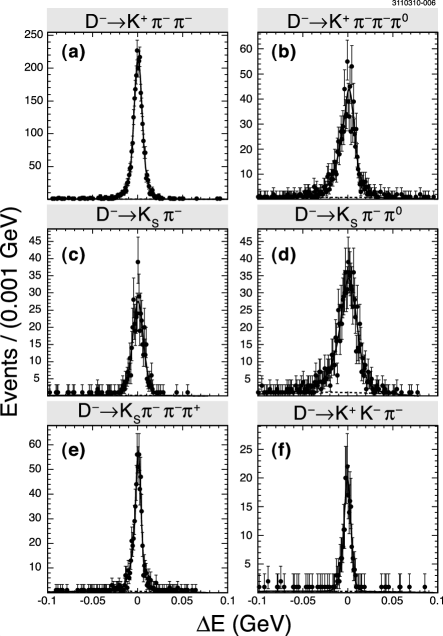
Figure 6: Distribution of $\Delta E$ for double tag events for the data, where $D^{-}$ candidate is reconstructed in one of the six tag modes [(a)–(f)], and $D^{+}$ candidate is reconstructed in $\bar{K}^{*0}e^{+}\nu_{e}$ mode. The points with error bars are the reconstructed yield from the data sample and the curves show our fit to the signal peak over the dashed background line.

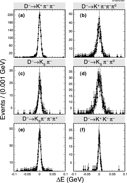
Figure 7: Distribution of $\Delta E$ for double tag events, where $D^{-}$ candidate is reconstructed in one of the six tag modes [(a)–(f)], and $D^{+}$ candidate is reconstructed in $\bar{K}^{*0}\mu^{+}\nu_{\mu}$ mode. The points with error bars are the reconstructed yield from the data sample and the curves show our fit to the signal peak over the dashed background line.

Figure 8: Results on the relative branching ratio, ${\mathcal{B}}_{\mu}/{\mathcal{B}}_{e}$ obtained for the six tag states and the error weighted average of these six values. We compare the relative branching ratio using the cross-feed method [Eq. (15)] to the ratio of absolute branching fractions. Table 3 gives a summary of these results.

Figure 8 and Table 3 compare our relative ${\mathcal{B}}_{\mu}/{\mathcal{B}}_{e}$ obtained using the cross-feed method to the ratio of absolute branching ratios for the six tag states and generic and SPD Monte Carlo simulations. The cross-feed method is reasonably consistent with the ratio of absolute branching fractions.

IV PROJECTIVE WEIGHTING TECHNIQUE

We extract the helicity basis form factors using the projective weighting technique more fully described in Ref. helicity-focus . For a given $q^{2}$ bin, a weight designed to project out a given helicity form factor, is assigned to the event depending on its $\theta_{\textrm{V}}$ and $\theta_{\ell}$ decay angles. We use 25 joint $\Delta\cos\theta_{\textrm{V}}\times\Delta\cos\theta_{\ell}$ angular bins: 5 evenly spaced bins in $\cos\theta_{\textrm{V}}$ times 5 bins in $\cos\theta_{\ell}$.

For each $q_{i}^{2}$ bin, we can write the bin populations $\vec{N}_{i}$ as a sum of the expected bin populations $\vec{m}_{\alpha}$ from each, individual form-factor product contribution to Eq. (LABEL:amp1). Thus $\vec{N}_{i}$ can be written as a linear combination with coefficients $f_{\alpha}(q_{i}^{2})$,

$$\vec{N}_{i}=f_{+}(q_{i}^{2})\,\vec{m}_{+}+f_{-}(q_{i}^{2})\,\vec{m}_{-}+f_{0}(q_{i}^{2})\,\vec{m}_{0}$$

$$+f_{I}(q_{i}^{2})\,\vec{m}_{I}+f_{T}(q_{i}^{2})\,\vec{m}_{T}+f_{TI}(q_{i}^{2})\,\vec{m}_{TI}\,.$$ (20)

Each of the six $f_{\alpha}(q_{i}^{2})$ coefficients is associated with one of the form factor products that we wish to measure. The six $\vec{m}_{\alpha}$ vectors are computed using SPD Monte Carlo simulations generated with the Eq. (LABEL:amp1) intensity but including just one of the six form factor products. For example, $\vec{m}_{+}$ is computed using a simulation generated with an arbitrary function for $H_{+}(q^{2})$ (such as $H_{+}(q^{2})=1$) and zero for the remaining five form factors. The $f_{\alpha}(q_{i}^{2})$ functions are proportional to the true $H^{2}_{\alpha}(q_{i}^{2})$ along with multiplicative factors such as $G_{F}^{2}\left|V_{cs}\right|^{2}(q^{2}-m_{\ell}^{2})$ and acceptance corrections.

Reference helicity-focus shows how Eq. (20) can be solved for the six form factor products $H_{+}^{2}(q^{2})$, $H_{-}^{2}(q^{2})$, $H_{0}^{2}(q^{2})$, $h_{0}(q^{2})H_{0}(q^{2})$, $H^{2}_{t}(q^{2})$, and $H_{0}(q^{2})H_{t}(q^{2})$ by making six weighted $q^{2}$ histograms. The weights are directly constructed from the six $\vec{m}_{\alpha}$ vectors.

Figure 9: Non-parametric form factor products obtained for the SPD Monte Carlo sample (multiplied by $q^{2}$) for ten, evenly spaced $q^{2}$ bins. The reconstructed form factor products are shown as the points with error bars, where the error bars represent the statistical uncertainties. The three points at each $q^{2}$ value are: filled circles a combined $D^{+}\rightarrow K^{-}\pi^{+}\mu^{+}\nu_{\mu}$ & $D^{+}\rightarrow K^{-}\pi^{+}e^{+}\nu_{e}$ sample, empty squares $D^{+}\rightarrow K^{-}\pi^{+}e^{+}\nu_{e}$ only, and empty triangles $D^{+}\rightarrow K^{-}\pi^{+}\mu^{+}\nu_{\mu}$ only. The solid curves represent our SPD model, which was used to generate the Monte Carlo sample. The histogram plots are: (a) $q^{2}H_{+}^{2}(q^{2})$, (b) $q^{2}H_{-}^{2}(q^{2})$, (c) $q^{2}H_{0}^{2}(q^{2})$, (d) $q^{2}h_{0}(q^{2})H_{0}(q^{2})$, (e) $q^{2}H^{2}_{t}(q^{2})$, and (f) $q^{2}H_{0}(q^{2})H_{t}(q^{2})$.

Figure 9 shows the six form factor products multiplied by $q^{2}$ obtained from a Monte Carlo simulation using our selection requirements. Because the isolated $D^{+}\rightarrow K^{-}\pi^{+}e^{+}\nu_{e}$ sample provides no useful information on the mass-suppressed form factor products $H^{2}_{t}(q^{2})$ and $H_{0}(q^{2})H_{t}(q^{2})$, the second point is not plotted for these two form factor products. The Monte Carlo sample was generated with our SPD Monte Carlo with $r_{3}=0$ and was run with three times our data sample. The reconstructed form factor products in the Monte Carlo simulation are a good match to the input model indicating that the projective weighting method is reasonably unbiased.

We turn next to a discussion of our normalization convention. Equation (13) tells us that as $q^{2}{}\rightarrow 0$, $q^{2}{}H_{\pm}^{2}(q^{2})\rightarrow 0$; and $q^{2}{}H^{2}_{0}(q^{2}){}$, $q^{2}{}h_{0}(q^{2})H_{0}(q^{2}){}$, $q^{2}{}H^{2}_{t}(q^{2})$, $q^{2}{}H_{0}(q^{2})H_{t}(q^{2}){}$ all approch the same constant. Therefore, we normalized the form factor products in Fig. 9 by scaling the weighted histograms by a single common factor so that $q^{2}{}H^{2}_{0}(q^{2}){}=1$ as $q^{2}{}\rightarrow 0$ based on the $q^{2}{}H^{2}_{0}(q^{2}){}$ measured in the combined $D^{+}\rightarrow K^{-}\pi^{+}e^{+}\nu_{e}$ and $D^{+}\rightarrow K^{-}\pi^{+}\mu^{+}\nu_{\mu}$ sample.

Figure 9 shows that the isolated $D^{+}\rightarrow K^{-}\pi^{+}\mu^{+}\nu_{\mu}$ and $D^{+}\rightarrow K^{-}\pi^{+}e^{+}\nu_{e}$ samples produce similar error bars for the measured $H^{2}_{+}(q^{2})$, $H^{2}_{-}(q^{2})$, and $h_{0}(q^{2})H_{0}(q^{2})$ form factor products, while the $H^{2}_{0}(q^{2})$ errors are much larger for the $D^{+}\rightarrow K^{-}\pi^{+}\mu^{+}\nu_{\mu}$ sample than for the $D^{+}\rightarrow K^{-}\pi^{+}e^{+}\nu_{e}$. This is due to the large correlation between the $H^{2}_{0}(q^{2})$ and $H^{2}_{t}(q^{2})$ form factors present in the $D^{+}\rightarrow K^{-}\pi^{+}\mu^{+}\nu_{\mu}$ sample owing to the similarity in their associated angular distributions. For this reason, the error bars on the $H^{2}_{t}(q^{2})$ form factor product are dramatically reduced when one combines the $D^{+}\rightarrow K^{-}\pi^{+}\mu^{+}\nu_{\mu}$ and $D^{+}\rightarrow K^{-}\pi^{+}e^{+}\nu_{e}$ samples.

V FORM-FACTOR RESULTS

We turn next to a discussion of our form-factor measurements. Figure 10 compares the $h_{0}(q^{2})H_{0}(q^{2})$ distribution below the nominal pole (a) to that above the nominal $K^{*0}$ pole (b). Figure 10 shows that there is no significant $h_{0}(q^{2})H_{0}(q^{2})$ signal above the $K^{*0}$ pole. The absence of a $h_{0}(q^{2})H_{0}(q^{2})$ signal above the nominal $K^{*0}$ shows that our data are consistent with the $\delta_{s}$ phase obtained in Refs. helicity-focus ; anomaly ; formfactor . A related interference pattern was observed in the FOCUS anomaly discovery of the $s$-wave interference in $D^{+}\rightarrow K^{-}\pi^{+}\mu^{+}\nu_{\mu}$ decay. We can thus improve our statistical errors by restricting our $h_{0}(q^{2})H_{0}(q^{2})$ measurements to events with $0.8<m_{K\pi}{}<0.9~{}\textrm{GeV}/c^{2}{}$. This additional requirement was applied to the $q^{2}h_{0}(q^{2})H_{0}(q^{2})$ plot of Fig. 11, while the other five form factor products use the full $0.8<m_{K\pi}{}<1.0~{}\textrm{GeV}/c^{2}{}$ mass range.

Figure 10: We show uncorrected plots of the $h_{0}(q^{2})H_{0}(q^{2})$ for data with $D^{+}\rightarrow K^{-}\pi^{+}\mu^{+}\nu_{\mu}$ and $D^{+}\rightarrow K^{-}\pi^{+}e^{+}\nu_{e}$ combined. (a) is for events below the nominal $K^{*0}$ pole: $0.8<m_{K\pi}{}<0.9~{}\textrm{GeV}/c^{2}{}$. (b) is for events above the nominal pole: $0.9<m_{K\pi}{}<1.0~{}\textrm{GeV}/c^{2}{}$. There is a strong $h_{0}(q^{2})H_{0}(q^{2})$ signal below the nominal pole but no evidence for a non-zero $h_{0}(q^{2})H_{0}(q^{2})$ form factor above the pole. Note the order of magnitude difference in the y-axis scales between the left and right plots.

Figure 11 shows the six form factor products multiplied by $q^{2}$ obtained for data using our $q^{2}{}H^{2}_{0}(q^{2}){}=1$ as $q^{2}{}\rightarrow 0$ normalization convention. The background was subtracted using our Monte Carlo samples. Although the data are a reasonably good match to the SPD model for the $q^{2}H_{0}^{2}(q^{2})$ and $q^{2}H_{\pm}^{2}(q^{2})$ form factors, the model does not match the data for $q^{2}h_{0}(q^{2})H_{0}(q^{2})$, and the mass-suppressed form factors $q^{2}H^{2}_{t}(q^{2})$ and $q^{2}H_{0}(q^{2})H_{t}(q^{2})$. These disagreements will be discussed in Sec. VI.

Figure 11: Non-parametric form factor products obtained for the data (multiplied by $q^{2}$) for ten evenly spaced $q^{2}$ bins. The reconstructed form factor products are shown as the points with error bars, where the error bars represent the statistical uncertainties. The three points at each $q^{2}$ value are: filled circles a combined $D^{+}\rightarrow K^{-}\pi^{+}\mu^{+}\nu_{\mu}$ & $D^{+}\rightarrow K^{-}\pi^{+}e^{+}\nu_{e}$ sample, empty squares $D^{+}\rightarrow K^{-}\pi^{+}e^{+}\nu_{e}$ only, and empty triangles $D^{+}\rightarrow K^{-}\pi^{+}\mu^{+}\nu_{\mu}$ only. The solid curves show our SPD model. The histogram plots are: (a) $q^{2}H_{+}^{2}(q^{2})$, (b) $q^{2}H_{-}^{2}(q^{2})$, (c) $q^{2}H_{0}^{2}(q^{2})$, (d) $q^{2}h_{0}(q^{2})H_{0}(q^{2})$, (e) $q^{2}H^{2}_{t}(q^{2})$, and (f) $q^{2}H_{0}(q^{2})H_{t}(q^{2})$.

Because of our excellent $q^{2}$ resolution, there is negligible correlation among the ten $q^{2}$ bins for a given form factor product, but the relative correlations between different form factor products in the same $q^{2}$ bin can be much larger. Most of the correlations are less than 30 %. There are, however, some very strong ($>70\%$) correlations for $H_{-}(q^{2})$ with various other form factors – most notably in the three lowest $q^{2}$ bins in the correlations between the $H_{-}(q^{2})$ and the $H_{T}~{}H_{0}$ as well as $H_{0}^{2}$ form factor products.

Table 4, a tabular representation of Fig. 11 for the $D^{+}\rightarrow K^{-}\pi^{+}\mu^{+}\nu_{\mu}$ and $D^{+}\rightarrow K^{-}\pi^{+}e^{+}\nu_{e}$ combined sample, gives the center of each $q^{2}$ bin, the measured form-factor product, its statistical uncertainty (first error) and its estimated systematic uncertainty (second error). The biggest source of the systematic uncertainty is from the background estimation. We separately consider systematic uncertainties from non-semileptonic decay backgrounds, and semileptonic decay backgrounds. The semileptonic backgrounds include cross-feed as well as semimuonic events where the pion and muon are exchanged.

For the background uncertainty, we assign a conservative systematic error by increasing the level of the non-semileptonic background and semileptonic background subtractions by a factor of 1.5 and comparing these form factor products to the results with the nominal background subtractions. For $H^{2}_{+}(q^{2})$ and $h_{0}(q^{2})H_{0}(q^{2})$, the non-semileptonic and semimuonic background subtraction systematic uncertainty is less than 20 % of the statistical error, while for the other four form factor products the systematic error is less than 40% of the statistical error.

We also assess a relative systematic error due to uncertainties in track reconstruction and particle identification efficiencies. The systematic uncertainty from this source is rather small since we are reporting form factor shapes rather than absolute normalization. This uncertainty is estimated as less than 1.9 % for all the form factor products. Finally, we assess a scale error of 13.4% on the $h_{0}(q^{2})H_{0}(q^{2})$ form factor product due to the uncertainties in the $A$ and $\delta$ values reported in Ref. formfactor . When this $s$-wave scale error is added in quadrature to the subtraction systematic error, the total systematic error rises to about 85% of the statistical error in the lowest three $q^{2}$ bins of the $h_{0}(q^{2})H_{0}(q^{2})$ form factor product, but systematic errors on the form factor shape are less than 20% of the statistical error.

Table 4: Summary of form factor product results for ten, evenly spaced $q^{2}$bins for the $D^{+}\rightarrow K^{-}\pi^{+}\mu^{+}\nu_{\mu}$ and $D^{+}\rightarrow K^{-}\pi^{+}e^{+}\nu_{e}$ combined sample. The first and second errors are statistical and systematical uncertainties, respectively. The numbers are normalized using the condition: $q^{2}{}H^{2}_{0}(q^{2}){}=1$ as $q^{2}{}\rightarrow 0$.

$q^{2}$	$q^{2}$ $H^{2}_{+}(q^{2})$	$q^{2}$ $H^{2}_{-}(q^{2})$	$q^{2}$ $H^{2}_{0}(q^{2})$
0.05	0.0013$\pm$0.0061$\pm$0.0010	0.0398$\pm$0.0304$\pm$0.0099	1.1979$\pm$0.0737$\pm$0.0276
0.15	0.0417$\pm$0.0135$\pm$0.0026	0.2467$\pm$0.0380$\pm$0.0146	1.0598$\pm$0.0616$\pm$0.0253
0.25	0.0993$\pm$0.0209$\pm$0.0036	0.4242$\pm$0.0471$\pm$0.0221	1.1160$\pm$0.0656$\pm$0.0274
0.35	0.1079$\pm$0.0259$\pm$0.0039	0.6704$\pm$0.0535$\pm$0.0175	1.0520$\pm$0.0690$\pm$0.0217
0.45	0.1401$\pm$0.0290$\pm$0.0031	0.8822$\pm$0.0575$\pm$0.0120	0.9556$\pm$0.0721$\pm$0.0203
0.55	0.2140$\pm$0.0358$\pm$0.0026	1.0809$\pm$0.0605$\pm$0.0025	1.0941$\pm$0.0832$\pm$0.0181
0.65	0.3874$\pm$0.0457$\pm$0.0057	1.2094$\pm$0.0692$\pm$0.0017	0.9692$\pm$0.0891$\pm$0.0165
0.75	0.3907$\pm$0.0548$\pm$0.0060	1.4181$\pm$0.0830$\pm$0.0085	1.0531$\pm$0.1030$\pm$0.0195
0.85	0.5670$\pm$0.0759$\pm$0.0090	1.2612$\pm$0.0982$\pm$0.0164	1.3298$\pm$0.1415$\pm$0.0307
0.95	0.7475$\pm$0.1495$\pm$0.0084	1.5113$\pm$0.1952$\pm$0.0263	1.4912$\pm$0.2539$\pm$0.0421
$q^{2}$	$q^{2}$ $h_{0}(q^{2})H_{0}(q^{2})$	$q^{2}$ $H^{2}_{t}(q^{2})$	$q^{2}$$H_{0}(q^{2})H_{t}(q^{2})$
0.05	1.5263$\pm$0.2649$\pm$0.2068	-0.1535$\pm$1.0530$\pm$0.2330	-0.4717$\pm$0.4033$\pm$0.1983
0.15	1.3410$\pm$0.2081$\pm$0.1802	0.3069$\pm$0.8381$\pm$0.3261	-1.1157$\pm$0.7390$\pm$0.3345
0.25	1.5601$\pm$0.2470$\pm$0.2092	-0.9425$\pm$1.0708$\pm$0.4993	-1.0842$\pm$0.8925$\pm$0.2879
0.35	0.3432$\pm$0.2450$\pm$0.0657	-2.8312$\pm$2.2685$\pm$1.1741	1.0604$\pm$1.2657$\pm$0.3050
0.45	1.0085$\pm$0.2927$\pm$0.1378	5.0488$\pm$3.2535$\pm$1.3110	1.4500$\pm$2.2843$\pm$0.5273
0.55	0.7593$\pm$0.3344$\pm$0.1186	-3.5770$\pm$4.0787$\pm$1.6076	-1.2391$\pm$3.1060$\pm$0.3136
0.65	0.5340$\pm$0.3524$\pm$0.0906	-0.1290$\pm$5.8905$\pm$2.2112	-1.1319$\pm$4.1718$\pm$0.2507
0.75	0.3474$\pm$0.3856$\pm$0.0758	6.2982$\pm$7.6928$\pm$2.1522	9.9457$\pm$7.8013$\pm$0.7991
0.85	-0.0682$\pm$0.3905$\pm$0.0538	-16.9593$\pm$10.8847$\pm$3.1543	-13.1707$\pm$11.6553$\pm$0.0672
0.95	0.1968$\pm$0.8383$\pm$0.0266	-75.1674$\pm$33.6395$\pm$4.8926	-2.1058$\pm$16.0185$\pm$0.0680

Figure 12 illustrates our sensitivity to the pole masses in Eq. (13) by comparing measurements of the $q^{2}~{}H^{2}_{-}(q^{2})$ form factor product to a model with spectroscopic axial and vector pole masses versus a model with infinite pole masses, implying constant axial and vector form factors. Our data favor the spectroscopic pole masses given in Eq. (14), for the high $q^{2}$ bins of the $H^{2}_{-}(q^{2})$ form factor product. The other five form factor products are consistent with either pole mass choice.

Figure 12: Evidence for finite pole masses. We show the measured $q^{2}H^{2}_{-}(q^{2}){}$ form factor shown in Fig. 11 overlayed with two models. (a) uses the same SPD model shown in Fig. 11 while (b) overlays the data with a SPD model where the axial and vector poles [$M_{A}$ and $M_{V}$ in Eq. (LABEL:amp1)] are set to infinity. We show the data with $D^{+}\rightarrow K^{-}\pi^{+}\mu^{+}\nu_{\mu}$ and $D^{+}\rightarrow K^{-}\pi^{+}e^{+}\nu_{e}$ combined. The slight scale difference between the data points in the two plots is an artifact of our $q^{2}{}H^{2}_{0}(q^{2}){}=1$ as $q^{2}{}\rightarrow 0$ normalization scheme, which is based on the two different pole mass predictions for the $H^{2}_{0}(q^{2})$ form factor product.

It is of interest to search for the possible existence of additional non-resonant amplitudes of higher angular momentum. It is fairly simple to extend Eq. (LABEL:amp1) to account for potential $d$-wave or $f$-wave interference with the $\overline{K}^{*0}$Breit-Wigner amplitude. We search specifically for a possible zero helicity $d$-wave or $f$-wave piece that interferes with the zero helicity $\overline{K}^{*0}$ contribution. One expects that such potential $h^{(d)}_{0}(q^{2})$ and $h^{(f)}_{0}(q^{2})$ form factors would peak as $1/\sqrt{q^{2}}$ near $q^{2}{}\rightarrow 0$ as is the case for the other zero helicity contributions $H_{0}(q^{2})$ and $h_{0}(q^{2})$. If so, the zero helicity contributions should be much larger than potential $d$- or $f$-wave $\pm 1$ helicity contributions. The $d$-wave projectors are based on an additional interference term of the form

$$4\,\sin^{2}\theta_{\ell}(3\,\cos^{2}\theta_{\textrm{V}}-1)\,H_{0}(q^{2})\,h^{(d)}_{0}(q^{2})\,{\mathop{\mathrm{Re}}\nolimits}\{A_{d}e^{-i\delta_{d}}\beta\}.$$ (21)

To search for the presence of zero helicity $d$-wave amplitude we use the technique of Ref. helicity-focus to construct a projector which is orthogonal to the projectors for each of the six terms in Eq. (LABEL:amp1). The $f$-wave weights are based on an additional interference term of the form

$$4\,\sin^{2}\theta_{\ell}(5\,\cos^{3}\theta_{\textrm{V}}-3\cos\theta_{\textrm{V}})\,H_{0}(q^{2})\,h^{(f)}_{0}(q^{2})\,{\mathop{\mathrm{Re}}\nolimits}\{A_{f}e^{-i\delta_{f}}\beta\}.$$ (22)

Averaging over the Breit-Wigner intensity, the interference should be proportional to $A_{d,f}\,\sin{\delta_{d,f}}\,h_{0}^{(d,f)}(q^{2})\,H_{0}(q^{2}){}$ and will disappear when the non-resonant amplitude is orthogonal to the average, accepted $\overline{K}^{*0}$ amplitude. Fig. 13 shows the $q^{2}{}h_{0}^{(d,f)}(q^{2})H_{0}(q^{2})$ form factor products obtained in the data using projective weights generated assuming a phase of zero. The projective weights are normalized so that $q^{2}{}h^{(d,f)}(q^{2})H_{0}(q^{2})=1$ in the limit $q^{2}\rightarrow 0$ if the putative $d$,$f$ -wave amplitude had the same strength as the $s$-wave amplitude relative to the $\overline{K}^{*0}$ Breit-Wigner amplitude.

Figure 13: Measurements of the $d$-wave form factor product (a) and $f$-wave form factor product (b) for an assumed phase of 0 radians relative to the $\overline{K}^{*0}$ Breit-Wigner amplitude.

There is no evidence for either a $d$-wave or $f$-wave component with this phase.

Figure 14: Search for d-wave, (a) and (b), and f-wave, (c) and (d), interference effects for each phase assumption as described in the text. The phases $\delta_{d}$ and $\delta_{f}$ represent the phase of possible d and f -wave contributions relative to the phase of the $\overline{K}^{*0}$Breit-Wigner amplitude. They are measured in radians.

Figure 14 shows our amplitude and limits for sixteen phase assumptions. As illustrated by Fig. 10, our ability to measure a non-resonant amplitude can depend critically on its phase relative to the average, accepted $\overline{K}^{*0}$ phase. In order to maximize our sensitivity to the non-resonant amplitude, for each phase assumption and $q^{2}$ bin we made our measurement based on three $m_{K\pi}$ mass regions: $0.8<m_{K\pi}<0.9~{}\textrm{GeV}/c^{2}$, $0.8<m_{K\pi}<1.0~{}\textrm{GeV}/c^{2}$, and $0.9<m_{K\pi}<1.0~{}\textrm{GeV}/c^{2}$, which puts the average $\overline{K}^{*0}$ reference phase at roughly $3\pi/4$, $3\pi/2$, and $7\pi/4$ for these three mass regions, respectively. We chose the mass region with the smallest expected error according to the Monte Carlo simulation. Under the assumption $h^{(d,f)}_{0}(q^{2}{})=H_{0}(q^{2}){}$, used in Ref. formfactor , we performed a $\chi^{2}$ fit of Fig. 13 to the form $A_{d,f}\,\sin{\delta_{d,f}}\,H^{2}_{0}(q^{2})$ over the region $q^{2}{}<0.6~{}\textrm{GeV}^{2}/c^{4}$ to find the amplitude and limits shown in Fig. 14.

Figure 14 shows that this “mass selection” method produced non-amplitude limits, which are reasonably independent of assumed phase. If, on the other hand, one used the full $0.8<m_{K\pi}<1.0~{}\textrm{GeV}/c^{2}$ mass range for all sixteen phase assumptions, one would get dramatically poorer limits for phase choices orthogonal to the Breit-Wigner amplitude phase. It is apparent from Fig. 14 that we have no compelling evidence for either a $d$-wave, or an $f$-wave component.

VI SUMMARY

We present a branching fraction and form factor analysis of the $D^{+}\rightarrow K^{-}\pi^{+}\ell^{+}\nu_{\ell}$ decay based on a sample of approximately 11800 $D^{+}\rightarrow K^{-}\pi^{+}e^{+}\nu_{e}$ and $D^{+}\rightarrow K^{-}\pi^{+}\mu^{+}\nu_{\mu}$ decays collected by the CLEO-c detector running at the $\psi(3770)$. We find ${\cal B}_{e}(D^{+}\rightarrow\overline{K}^{*0}e^{+}\nu_{e}{})=(5.52\pm 0.07\pm 0.13)\%$ and ${\cal B}_{\mu}(D^{+}\rightarrow\overline{K}^{*0}\mu^{+}\nu_{\mu})=(5.27\pm 0.07\pm 0.14)\%$. Our direct measurement of the relative semimuonic to semielectric branching ratio using Eq. (15) is ${\mathcal{B}}_{\mu}/{\mathcal{B}}_{e}{}=(94.64\pm 1.95\pm 1.03)\%$.

We also present a non-parametric analysis of the helicity basis form factors that control the kinematics of the $D^{+}\rightarrow K^{-}\pi^{+}\ell^{+}\nu_{\ell}$ decays. We used a projective weighting technique that allows one to determine the helicity form factor products by weighted histograms rather than likelihood based fits. We find consistency with the spectroscopic pole dominance model for the dominant $H^{2}_{+}(q^{2})$, $H^{2}_{-}(q^{2})$ and $H^{2}_{0}(q^{2})$ form factors. Our measurement on the $h_{0}(q^{2})H_{0}(q^{2})$ form factor product suggests that the $h_{0}$ form factor falls faster than $H_{0}$ with increasing $q^{2}$. The form factors determined using $D^{+}\rightarrow K^{-}\pi^{+}\mu^{+}\nu_{\mu}$ decays are consistent with those determined using $D^{+}\rightarrow K^{-}\pi^{+}e^{+}\nu_{e}$ decays and are consistent with our earlier study oldff of $D^{+}\rightarrow K^{-}\pi^{+}e^{+}\nu_{e}$. Our measured $H^{2}_{-}(q^{2})$ form factor data are more consistent with axial and vector form factors with the expected spectroscopic pole dominance $q^{2}$ dependence than with constant axial and vector form factors.

Our measurements of the $H^{2}_{t}(q^{2})$ and $H_{0}(q^{2})H_{t}(q^{2})$ form factor suggests a much smaller $H_{t}(q^{2})$ form factor than expected in Lattice Gauge Theory models lqcd . Within the context of the spectroscopic pole dominance model Eq. (14), our $H_{0}(q^{2})H_{t}(q^{2})$ measurements are most consistent with a small $H_{t}(q^{2})$ form factor contribution implying a very negative value for $r_{3}\equiv A_{3}(0)/A_{1}(0)$, such as $r_{3}=-10$, which would place the predicted ${\mathcal{B}}_{\mu}/{\mathcal{B}}_{e}$ relative branching ratio close to the phase space estimate of 91%. Finally, we have searched for possible $d$-wave or $f$-wave non-resonant interference contributions to $D^{+}\rightarrow K^{-}\pi^{+}\ell^{+}\nu_{\ell}$. We have no statistically significant evidence for $d$-wave or $f$-wave interference, but are only able to limit these terms to roughly less than 1.0 and 1.5 times the observed $s$-wave interference for $d$-wave and $f$-wave respectively.

References

(1)
S. Bianco, F.L. Fabbri, D. Benson, and I. Bigi, Riv. Nuovo Cim. 26N7,
1 (2003).
(2)
M. Bauer, B. Stech, and M. Wirbel, Z. Phys. C 29, 637 (1985);
M. Bauer and M. Wirbel, Z. Phys. C 42, 671 (1989);
J.G. Korner and G.A. Schuler, Z. Phys. C 46, 93 (1990);
F.J. Gilman and R.L. Singleton, Phys. Rev. D 41, 142 (1990);
D. Scora and N. Isgur, Phys. Rev. D 52, 2783 (1995);
B. Stech, Z. Phys. C 75, 245 (1997);
D. Melikhov and B. Stech, Phys. Rev. D 62, 014006 (2000).
(3)
P. Ball, V.M. Braun, H.G. Dosch, and M. Neubert, Phys. Lett. B 259,
481 (1991);
P. Ball, V.M. Braun, and H.G. Dosch, Phys. Rev. D 44, 3567 (1991).
(4)
C.W. Bernard, A.X. El-Khadra, and A. Soni, Phys. Rev. D 45, 869
(1992);
V. Lubicz, G. Martinelli, M.S. McCarthy, and C.T. Sachrajda, Phys. Lett. B
274, 415 (1992);
A. Abada et al., Nucl. Phys. B 416, 675 (1994);
K.C. Bowler et al. (UKQCD Collaboration), Phys. Rev. D 51, 4905 (1995);
T. Bhattacharya and R. Gupta, Nucl. Phys. B (Proc. Suppl.) 47, 481
(1996);
C.R. Alton et al. (APE Collaboration), Phys. Lett. B 345, 513 (1995);
S. Gusken, G. Siegert, and K. Schilling, Prog. Theor. Phys. Suppl. 122,
129 (1996);
A. Abada et al. (SPQcdR Collaboration), Nucl. Phys. Proc. Supp. 119, 625
(2003).
(5)
C. Bourrely, B. Machet and E. de Rafael, Nucl. Phys. B 189, 157 (1981);
C. G. Boyd, B. Grinstein and R. F. Lebed, Phys. Rev. Lett. 74, 4603 (1995);
L. Lellouch, Nucl. Phys. B 479, 353 (1996);
C. G. Boyd, B. Grinstein and R. F. Lebed, Nucl. Phys. B 461, 493 (1996);
I. Caprini and M. Neubert, Phys. Lett. B 380, 376 (1996);
I. Caprini, L. Lellouch and M. Neubert, Nucl. Phys. B 530, 153 (1998);
C. G. Boyd and M. J. Savage, Phys. Rev. D 56, 303 (1997);
M. Fukunaga and T. Onogi, Phys. Rev. D 71, 034506 (2005);
C. M. Arnesen, B. Grinstein, I. Z. Rothstein and I. W. Stewart, Phys. Rev. Lett. 95, 071802 (2005);
T. Becher and R. J. Hill, Phys. Lett. B 633, 61 (2006).
(6)
S. Fajfer and J. Kamenik, Phys. Rev. D 72, 034029 (2005).
(7)
J.M. Link et al. (FOCUS Collaboration), Phys. Lett. B 633, 183 (2006).
(8)
J.M. Link et al. (FOCUS Collaboration), Phys. Lett. B 535, 43 (2002).
(9)
J.M. Link et al. (FOCUS Collaboration), Phys. Lett. B 544, 89 (2002).
(10)
J.G. Korner and G.A. Schuler, Z. Phys. C 46, 93 (1990);
Fredrick J. Gilman
and Robert L. Singleton, Jr. Phys. Rev. D 41, 142 (1990)
(11)
Y. Kubota et al. (CLEO Collaboration), Nucl. Instrum. Methods A 320, 66 (1992);
M. Artuso et al., Nucl. Instrum. Methods A 554, 147 (2005);
D. Peterson et al., Nucl. Instrum. Methods A 478, 142 (2002).
(12)
S. Dobbs et al. (CLEO Collaboration), Phys. Rev. D 76, 112001 (2007).
(13)
D.J. Lange, Nucl. Instrum. Methods A 462, 152
(2001).
(14)
R. Brun et al., Geant 3.21, CERN Program Library Long Writeup W5013,
unpublished.
(15)
G.S. Hung et al. (CLEO Collaboration) Phys. Rev. Lett. 95, 181801 (2005).
(16)
C. Amsler et al. (Particle Data Group), Phys. Lett. B 667, 1 (2008).
(17)
M.R. Shepherd et al. (CLEO Collaboration), Phys. Rev. D 74, (2006) 052001.