Statistical characterization of temperature patterns in anisotropic cosmologies

Abstract

We consider the issue of characterizing the coherent large-scale patterns from CMB temperature maps in globally anisotropic cosmologies. The methods we investigate are reasonably general; the particular models we test them on are the homogeneous but anisotropic relativistic cosmologies described by the Bianchi classification. Although the temperature variations produced in these models are not stochastic, they give rise to a “non–Gaussian” distribution of temperature fluctuations over the sky that is a partial diagnostic of the model. We explore two methods for quantifying non–Gaussian and/or non-stationary fluctuation fields in order to see how they respond to the Bianchi models. We first investigate the behavior of phase correlations between the spherical harmonic modes of the maps. Then we examine the behavior of the multipole vectors of the temperature distribution which, though defined in harmonic space, can indicate the presence of a preferred direction in real space, i.e. on the 2-sphere. These methods give extremely clear signals of the presence of anisotropy when applied to the models we discuss, suggesting that they have some promise as diagnostics of the presence of global asymmetry in the Universe.

1 Introduction

Observations of the Cosmic Microwave Background (CMB) provide some of the most compelling support for the currently favored $\Lambda$CDM, or concordance, cosmological model. The concordance framework predicts that the CMB should posses temperature fluctuations which are both statistically isotropic (i.e. stationary over the celestial sphere) and Gaussian (Guth & Pi, 1982; Starobinskij, 1982; Bardeen, Steinhardt & Turner, 1983). Measurements by the Wilkinson Microwave Anisotropy Probe (WMAP) (Bennett et al., 2003; Hinshaw et al., 2009) have undergone extensive statistical analysis, much of which has confirmed the concordance model but with some indications of departures that may be significant; see for example Yadav & Wandelt (2008). More specifically, there is some evidence for hemispherical power asymmetry (Eriksen et al., 2004; Park, 2004; Eriksen et al., 2007; Hoftuft et al., 2009; Hansen et al., 2009) and also a Cold Spot has been identified (Vielva et al., 2004; Cruz et al., 2005). In other words there is some evidence of an anisotropic universe, i.e. one in which the background cosmology may not be described by the standard Friedman-Robertson-Walker (FRW) metric. Of course the background cosmology for a non-isotropic universe may still be described by the FRW metric, but this would require a non-standard topology which we do not consider in this analysis.

The Bianchi classification provides a complete characterization of all the known homogeneous but anisotropic exact solutions to General Relativity. The classification was first proposed by Bianchi and later applied to General Relativity (Ellis & MacCallum, 1969). Initial studies used the lack of large-scale asymmetry in the CMB temperature to put strong constraints on the possible Bianchi models (Barrow, Juszkiewicz & Sonoda, 1985; Bunn, Ferreira & Silk, 1996; Kogut, Hinshaw & Banday, 1997). However, simulations of the CMB from Bianchi universes not only show a preferred direction, but models with negative spatial curvature (such as the types V and VII_h) can produce localized features (Barrow, Juszkiewicz & Sonoda, 1985). So more recently attention has shifted to reproducing a Cold Spot such as that claimed to exist in the WMAP data. Initially, Type VII_h was the favored model to best reproduce the anomaly (Jaffe et al., 2005, 2006a, 2006b), and this has subsequently been investigated quite thoroughly (McEwen et al., 2006; Bridges et al., 2008; Pontzen & Challinor, 2007; Pontzen, 2009; Sung & Coles, 2010), although more recent work has also looked at the Bianchi Type V which also produces localized features (Sung & Coles, 2009).

The most interesting range of anisotropic structures is produced in Bianchi Types VII_h, VII₀ and V. These different Bianchi types have the effect of focusing and/or twisting the initial quadrupole over time (see Figure 1). In this paper we study the behavior of these Bianchi models so as to identify characteristics of the radiation fields they produce and develop methods that can be used to identify more general forms of anisotropy. Understanding the characteristics identified in these particular cases will hopefully help us find better and more systematic ways of constraining the level of global symmetry present in the real Universe. Note we consider just characteristics observable in the CMB temperature; we shall return to a study of the polarization radiation component in later work.

We consider two statistical measures of anisotropy in some detail in this paper. Neither of these is entirely new and both have previously been applied to observed CMB maps. However, the general philosophy behind previous applications of these methods has been simply to look for departures from the (composite) null hypothesis of statistical isotropy and Gaussianity (or more recently they have been developed to look at universes with multiply-connected topologies (Bielewicz & Riazuelo, 2009)). In other words, they have been used to construct hypothesis tests with the concordance cosmology but their performance has not hitherto been evaluated on models with built-in anisotropy.

For example, if the concordance model is correct, the phases of the spherical harmonic coefficients of the CMB should be independently random and uniformly distributed. Recent studies have suggested some deviation from this (Coles et al., 2004; Stannard & Coles, 2005; Dineen, Rocha & Coles, 2005; Chiang, Naselsky & Coles, 2007; Chiang et al., 2007) but it is not clear whether they indicate global anisotropy or departures from Gaussianity, let alone whether these are of cosmic or instrumental origin. Here we examine the use of phase correlations in quantifying the temperature patterns generated in models with known levels of global inhomogeneity.

Multipole vectors were first introduced over a century ago (Maxwell, 1891). There have since been attempts to understand the multipole vectors in order to explain the CMB anomalies reported at large angular scales (Katz & Weeks, 2004; Schwarz et al., 2004; Copi, Huterer & Starkman, 2004; Land & Magueijo, 2005a, b, c, d, e; Copi et al., 2006, 2007) since is not clear how to quantify and verify such properties from the CMB anomalies in spherical harmonics. They have been used in a number of studies to show anomalies, such as alignments of multiples (Abramo et al., 2006) in a similar plane to the axis of evil (Land & Magueijo, 2005d, 2007). Our aim here is to examine the behavior of the multipole vectors in cases where the form of anisotropy is known priori in order to assess their potential to act as more general descriptors.

Two points are worth making before we continue. First, any realistic cosmology (whether of FRW or Bianchi type) will possess random fluctuations on top of a smooth background. If these fluctuations are stationary Gaussian then they will add correlated “noise” to any signal arising from the background model and will thus hamper the performance of any statistical analysis method, especially at smaller angular scales. This Gaussian “noise” (which is equivalent to stationary Gaussian fluctuations, and not to be confused with instrumental noise) is completely characterized by second-order statistical quantities (i.e. the power spectrum in harmonic space or the autocorrelation function in pixel space). The statistical descriptors we explore are independent of the power-spectrum, so adding Gaussian noise will not produce any systematic response in them.

We also restrict ourselves to looking at just the large-scale features because the patterns in the temperature maps resulting from the Bianchi models is over large scales. Therefore, by looking at large scales only, there is more chance of detecting the anisotropy. However, it goes without saying we are not claiming that these Bianchi models are in themselves complete alternatives to the concordance cosmology. Rather we think of them as representing possible perturbation modes of the FRW background.

The layout of this article is as follows. In Section 2 we look at pixel distributions of the CMB maps to show how the statistical anisotropy present in these models produces a form of non-Gaussianity in the pixel distribution over the celestial sphere. We then introduce phase correlations in Section 3 to provide characterization of the anisotropy displayed by the models. In Section 4 we look at the behavior of the multipole vectors as characteristics of the anisotropy of the same maps. Finally, Section 5 summarizes the conclusions.

.

Figure 1: Simulated maps of the the CMB temperature, at redshift z = 0, using Bianchi type cosmologies. From left to right the Bianchi types are: V, VII₀ and VII_h. The colour scale is marked in milliKelvin. All the maps started as a quadruple at z = 500. The Bianchi V map shows a focused feature, the Bianchi VII₀ map has a twisted feature and the Bianchi VII_h map has both focusing and twisting in the resulting temperature pattern.

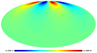
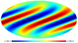
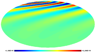
2 Statistical Descriptors of non-Gaussianity

Sung & Coles (2009) discussed how localized features in the CMB temperature pattern, perhaps similar to the Cold Spot observed in the WMAP data (Vielva et al., 2004; Cruz et al., 2005), can be generated in models with negative spatial curvature, i.e. Bianchi types V and VII_h. In the standard cosmological framework the temperature fluctuations are described by a Gaussian random process over the sky, so a feature like the cold spot corresponds to an extreme event in the tail of the distribution of fluctuations. In a Bianchi model, however, it is not stochastic at all but produced coherently as a result of the geometry of the space-time.

Clearly we need a systematic way to characterize the relationship between rare events like this and their origin through either non-Gaussianity or global anisotropy. Analysis of the temperature patterns using standard descriptors in non-standard scenarios will produce signals different from what one would see in the presence of stationary Gaussian noise. To illustrate this issue we study the pixel distribution function of temperature values. This is an obvious way to test for non-Gaussianity in a random field of temperature values, but a coherent fluctuation field also possesses a one-point distribution that yields some diagnostic information. In this sense, all the Bianchi models are inherently non-Gaussian but their non-Gaussianity is simply a manifestation of the presence of anisotropy.

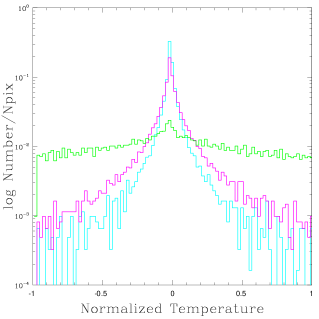
We calculated the pixel distribution function, which is simply a frequency count of the pixel (or temperature) values, for each of the Bianchi maps and used it to plot the histogram seen in Figure 2. A perfectly homogeneous and isotropic map, such as that predicted by the concordance model, would have a constant value over the whole map - remember we are considering maps without fluctuations - and therefore a histogram of the pixel distribution histogram for this map would give a delta function at the mean. Our results show some deviation from this prediction. In Figure 2 we see the plots for the Bianchi V and VII_h types have strongly peaked features at the mean, but still with some non zero variance; the type VII₀ model has a nearly uniform distribution across the whole temperature range.

Although not demonstrated in this diagram, another point to note is that at early times the histograms of the pixel distribution functions of the three different Bianchi types are almost identical; the different values of the temperature pixels are roughly even over the range. As redshift decreases, the temperature patterns for Bianchi V and VII_h gradually start to focus (see Sung & Coles, 2009), and their histograms of the pixel distribution functions become successively more peaked. For the Bianchi type VII₀ the temperature pattern just twists, reorganizing the pattern on the sky while the histogram stays roughly the same. These observations help to explain the features in the histograms. As the temperature patterns become more focused, more of the rest of the map becomes uniform and so the histogram is tending towards a delta function.

In summary, what we would hope to discover from the pixel distribution histogram is that it gives us some clues about the homogeneity and isotropy of the maps i.e. the degree of concentration around the mean might tells us about the homogeneity of the parameters or the asymmetry of the distribution might give information about the anisotropy. But as it stands, the information from the pixel distribution function is not that clear. All we can say is that the histograms differ from a delta function, so the maps are not perfectly homogeneous and isotropic, and that the histograms are clearly non-Gaussian in shape. However the shape of this one-point pixel distribution does not furnish us with a complete description of the pattern because it does not take into angular correlations between the pixels.

Figure 2: The pixel distribution function of the normalized temperature for the Bianchi CMB maps. The y axis indicates the normalized pixel number which is the whole range of temperature covered by the plot, but normalized so they can be plotted on the same axes. The colour cyan represents type V, magenta for VII_h, and green for VII₀. The plot shows that the Bianchi V and VII_h types have strongly peaked features at the mean, whereas the type VII₀ has a nearly uniform distribution across the temperature range.

3 Phase correlations of Bianchi CMB Maps

We now move on from pixel distributions to consider the spherical harmonics of the temperature maps, or more specifically the phases of the spherical harmonic coefficients.

3.1 Spherical Harmonics

The temperature of the CMB, $T_{\theta,\phi}$, is defined on a sphere where $\theta\in[0,\pi]$ and $\phi\in[0,2\pi]$ are the polar and azimuthal angles. Therefore one way of describing the temperature anisotropies, $\Delta T_{\theta,\phi}$, is to extract the corresponding spherical harmonic coefficients ($a_{{{\ell}m}}$):

$$\Delta T_{\theta,\phi}=\frac{T_{\theta,\phi}-\bar{T}}{\bar{T}}=\sum_{\ell=0}^{\infty}\sum_{m=-\ell}^{\ell}|a_{{{\ell}m}}|e^{i\Phi_{{{\ell}m}}}Y_{{{\ell}m}}(\theta,\phi),$$ (1)

where $|a_{{{\ell}m}}|$ and $\Phi_{{{\ell}m}}$ are the amplitudes and phases of the spherical harmonic coefficients, and $Y_{{{\ell}m}}$ are the spherical harmonics which are defined here as:

$$Y_{{{\ell}m}}=(-1)^{m}\sqrt{\frac{2{\ell}+1}{4\pi}\frac{({\ell}-m)!}{({\ell}+m)!}}P_{{{\ell}m}}(\cos\theta)e^{im\phi},$$ (2)

where $P_{{{\ell}m}}$ is the associated Legendre Polynomial. Note that this definition of spherical harmonics includes a phase factor of $(-1)^{m}$, also known as the Condon-Shortley phase.

In the standard cosmological model, the temperature fluctuation field is produced by stochastic fluctuations which are Gaussian and statistically stationary over the celestial sphere. In this case the phases $\Phi_{{{\ell}m}}$ of each spherical harmonic mode $a_{{{\ell}m}}$ are independent and uniformly random on the interval $[0,2\pi]$ (Coles et al., 2004). If instead the temperature pattern on the sky is produced by a Bianchi geometry then the $a_{{{\ell}m}}$ are no longer stochastically generated but can be directly calculated from parameters of the model. Analytical forms for the temperature pattern can be used to obtain the spherical harmonic phases (McEwen et al., 2006; Bridges et al., 2008), but it is clumsy to transform these between different coordinate systems (Coles et al., 2004). In the following we therefore obtain distributions of $\Phi_{{{\ell}m}}$ from Bianchi maps generated using the method described by Sung & Coles (2010).

3.2 Visualising phase correlations

To visualize the information held in the phases, $\Phi_{{{\ell}m}}$, of the spherical harmonic coefficients, $a_{{{\ell}m}}$, we plotted them over all ${\ell}$ and $m$. Rather than using a 3D plot, colour has been used to represent the $\Phi_{{{\ell}m}}$ following Coles & Chiang (2000). The colours equate to the angle on a colour wheel: red ($\Phi_{{{\ell}m}}=0$), green ($\Phi_{{{\ell}m}}=\pi/2$), cyan ($\Phi_{{{\ell}m}}=\pi$), and purple ($\Phi_{{{\ell}m}}=3\pi/2$). To understand these plots, first consider what we would expect to see in the case of an isotropic and homogeneous universe as predicted by the concordance model. This would be a uniform map (as we are not at this point considering fluctuations) but in spherical harmonics this only has power in one mode (${\ell}=m=0$), so there is no phase for the other modes. Better to consider a map with Gaussian fluctuations as later in the section we will move on to add noise to the Bianchi maps. Figure 3 shows the phases ($\Phi_{{{\ell}m}}$) for a homogeneous and isotropic map with Gaussian fluctuations. The phases are random over the space i.e. there are no visible patterns in the distribution of colours in the plot. Note that for all the maps, $\Phi_{{{\ell}m}}$ = 0 or $\pi$ for $m$ = 0 because the $a_{{{\ell}m}}$ coefficients are defined so that $a_{{{\ell}m}}=a_{l,-m}$. Other than this, the distribution of $\Phi_{{{\ell}m}}$ is random. Also, note that for all $|m|>{\ell}$, $\Phi_{{{\ell}m}}$ = 0.

Figure 3: Example of the spherical harmonic phases ($\Phi_{{{\ell}m}}$) we would expect for the concordance model where ${\ell}$, $m$ $\in$ [0, 20]. The distribution of $\Phi_{{{\ell}m}}$ is random, apart from for $m=0$, where the phases can only be 0 or $\pi$ by definition. The colours represent the different values of the $\Phi_{{{\ell}m}}$ (red ($\Phi_{{{\ell}m}}=0$), green ($\Phi_{{{\ell}m}}=\pi/2$), cyan ($\Phi_{{{\ell}m}}=\pi$), and purple ($\Phi_{{{\ell}m}}=3\pi/2$)).

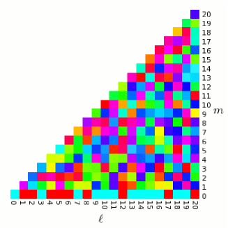
We extracted the $\Phi_{{{\ell}m}}$ from each of the Bianchi maps using Healpix (Górski et al., 2005) and plotted them in the same way as we have described; the results are shown in Figure 5. The plots show that the $\Phi_{{{\ell}m}}$ are not random but have patterns, i.e. the harmonic modes manifest some form of phase correlation. For all the Bianchi types, $\Phi_{{{\ell}m}}$ = 0 for all odd $m$. For the VII₀ and V types, all the $\Phi_{{{\ell}m}}$ are orthogonal i.e. they are either 0, $\pi/2$, $\pi$, or $3\pi/2$. Both the VII₀ and VII_h types show sequences of increasing/decreasing phases, which are particularly prominent for $m=2$.

Figure 4: Phases of the spherical harmonic coefficients ($\Phi_{{{\ell}m}}$) for Bianchi types V (left), VII₀ (middle) and VII_h (right) where ${\ell}$, $m$ $\in$ [0, 20] and z = 0. Note that ${\ell}$ is plotted against the x axis, increasing from left to right, and $m$ is plotted against the y axis, increasing from bottom to top. The distributions are not random (as in Figure 3) but exhibit some distinctive features. All the $\Phi_{{{\ell}m}}$ for the VII₀ and V types are orthogonal, and there are sequences of colours in the type VII_h (see $m=2$).

Figure 5: $\Delta\Phi_{{{\ell}m}}$ for Bianchi types V (left), VII₀ (middle) and VII_h (right) where ${\ell}$, $m$ $\in$ [0, 20] and z = 0. Note that ${\ell}$ is plotted against the x axis, increasing from left to right, and $m$ is plotted against the y axis, increasing from bottom to top. Like the phases (Figure 5) the distributions are not random but exhibit some distinctive features. All the $\Delta\Phi_{{{\ell}m}}$ for the V type are either 0 or $\pi$. The $\Delta\Phi_{{{\ell}m}}$ for the VII₀ type are again orthogonal but in a more correlated way. Similarly, the sequences of colours in the type VII_h are now even more prominent (see $m=2$).

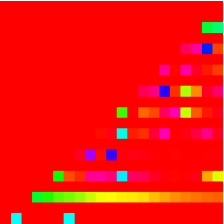
While some patterns are apparent in these plots, an even better way to visualize the phase correlations is to look at the phase differences which are defined here as:

$$\Delta\Phi_{{{\ell}m}}=\Phi_{{{\ell}m}}-\Phi_{{\ell},m-1}$$ (3)

The phase differences are shown in Figure 5 and the correlations are much more apparent compared to the plots of $\Phi_{{{\ell}m}}$. All the $\Delta\Phi_{{{\ell}m}}$ for the V type are lined up, i.e. either 0 or $\pi$. The $\Delta\Phi_{{{\ell}m}}$ for the VII₀ type are again orthogonal, but whereas in the phases the distribution of 0, $\pi/2$, $\pi$, and $3\pi/2$ seemed some what random, in the phase differences we see similar values ‘clump’ together. Similarly, the sequences of colours in the type VII_h (see $m=2$ for example) are now even more prominent.

So, strong correlations are observed in the phases and phases differences of the simulated Bianchi CMB maps. But we have only looked at large angular scales where there are only a small number of independent data points. Even without noise, it is important to ask the question whether these correlations are likely to be statistically significant. One way to quantify this is to use a Kolmogorov-Smirnov test. This is a non-parametric statistical test which measures the maximum distance of a given distribution from a reference probability distribution. In this case we want to show deviation from a random set of $\Delta\Phi_{{{\ell}m}}$, i.e. a uniform distribution, which is predicted by the concordance model.

To calculate the Kolmogorov-Smirnov test statistic a set of phase differences $\Delta\Phi_{{{\ell}m}}$ are separated into bins of equal size between 0 and $2\pi$. The number of $\Delta\Phi_{{{\ell}m}}$ which fall into each bin are counted and a cumulative distribution derived. If the distribution is uniform, as in the case of the reference probability distribution, then the number of $\Delta\Phi_{{{\ell}m}}$ in each of the bins should increase roughly linearly across the bins. The difference between both the sample and uniform cumulative distributions is found for each bin and the biggest difference is the Kolmogorov-Smirnov statistic D.

To deduce the significance of D, a set of ten thousand tests have been run to generate sets of random angles of equal size to the sample sets. D was found for each of these sets and this data was used to find the significance of D for the sample distributions from the Bianchi maps.

The Kolmogorov-Smirnov statistic D, and the derived probability of that statistic P(D), for all the Bianchi maps are detailed in Table 1.

Map	z	D	P(D) %
VIIh	500	0.11	94.5
VIIh	200	0.09	77.1
VIIh	60	0.14	99.2
VIIh	10	0.24	$>$99.9
VIIh	3	0.27	$>$99.9
VIIh	1	0.38	$>$99.9
VIIh	0	0.27	$>$99.9
VII0	0	0.28	$>$99.9
V	0	0.73	$>$99.9

Table 1: Results from the Kolmogorov-Smirnov test comparing the distribution of phase differences in the Bianchi CMB maps with a random distribution of phases as predicted by the concordance model. D is the Kolmogorov-Smirnov statistic found by comparing the phase differences $(\Delta\Phi$). $P(\textbf{{D}})$ is the Monte Carlo estimate of the probability of getting the value of D, or less, found for the Bianchi models, from a random selection of phase differences. These are computed by forming an empirical distribution of D from sets of random simulations and counting what fraction of the ensemble gives the results obtained for the Bianchi maps. For example, in the case of the $P(\textbf{{D}})$ for the VII_h map (z = 500) we find that, out of 10000 simulations, 9450 have a value of D less than 0.11. Given the probable sampling accuracy of around one percent, we have rounded the results.

This table shows that there is indeed a significant deviation from a uniform distribution for the phase differences for all Bianchi types. Of the 10000 random sets of data, none showed a value for D as high as seen for the Bianchi cases.

The Bianchi VII_h type was also considered at different redshifts to see how the correlations changed with time. Table 1 shows that in general value of D gets more significant over time i.e. the correlations in the phase differences of the Bianchi maps become stronger over time.

3.3 Rotating maps and adding noise

In Section 3.2 we applied the Kolmogorov-Smirnov test to a “clean” map that is perfectly aligned with the vertical axis. This section addresses how noise and rotation affect the identification of correlations in the phases of the spherical harmonics of CMB maps from Bianchi models.

First we consider rotation. Phases of spherical harmonic coefficients are not rotation-invariant. Rotating the coordinate system used to represent a CMB map in $\phi$ (which is equivalent to rotation around the z axis) would increment each of the spherical harmonic phases by $\phi$, so the phase differences would remain the same. Therefore rotation in $\phi$ would have no effect on the value of the Kolmogorov-Smirnov statistic D. Rotation in $\theta$ is more complicated to express so we used an empirical approach to quantity the effect on D. The Bianchi CMB maps were rotated by a small angle, $\theta=\pi/8$, and then the spherical harmonic coefficients were derived and used to calculate D. The results in Table 2 show that the values of D for each of the maps are even higher than in maps that hadn’t been rotated, indicating the presence of even stronger correlations. This suggests that, at least for small rotations off the axis, the correlations are just as significant, if not more so.

Map	z	D	P(D) %
VIIh	0	0.46	$>$99.9
VII0	0	0.38	$>$99.9
V	0	0.77	$>$99.9

Table 2: Results from the Kolmogorov-Smirnov test comparing the distribution of phase differences in the Bianchi CMB maps, rotated by $\theta=\pi/8$, with a random distribution of phase differences as predicted by the concordance model. D is the Kolmogorov-Smirnov statistic found when considering the phase differences. $P(\textbf{{D}})$ is the Monte Carlo estimate of the probability of getting the value of D, or less, found for the Bianchi models, from a random selection of phase differences. These are computed by forming an empirical distribution of D from sets of random simulations and counting what fraction of the ensemble gives the results obtained for the Bianchi maps. For example, in the case of the $P(\textbf{{D}})$ for the VII_h map we find that, out of 10000 simulations, over 9999 have a value of D less than 0.46.

As an aside, the colour plots of the phase differences for Bianchi maps rotated by a number of different $\theta$ in the range 0 to 2$\pi$ were generated. These plots have been condensed together into movies which show that the correlations in the VII₀ and V maps are visible across all $\theta$ and for the VII_h map are visible within about $\pi/3$ of the preferred axis. .

Figure 6: $\Delta\Phi_{{{\ell}m}}$ for ${\ell}$, $m\in$ [0, 20] (Bianchi type V map at z = 0 with white (left), WMAP (middle), and $\Lambda$CDM fluctuations (right) noise maps , $\theta=\pi/8$). Note that ${\ell}$ is plotted against the x axis, increasing from left to right, and $m$ is plotted against the y axis, increasing from bottom to top. Correlations can still be observed as lines of similar colours.

Map	z	Dwhite	P(D)%	Dwmap	P(D)%	DΛCDM	P(D)%
VIIh	0	0.15	99.2	0.16	99.8	0.17	99.8
VII0	0	0.09	77.1	0.08	66.1	0.07	52.0
V	0	0.19	$>$99.9	0.18	99.9	0.14	98.2

Table 3: Results from the Kolmogorov-Smirnov test comparing the distribution of phase differences in the Bianchi CMB maps rotated by $\theta=\pi/8$ with white, WMAP, and $\Lambda$CDM noise maps (z = 0) . D is the Kolmogorov-Smirnov statistic found when considering the phase differences. $P(\textbf{{D}})$ is the Monte Carlo estimate of the probability of getting the value of D, or less, found for the Bianchi models, from a random selection of phase differences. These are computed by forming an empirical distribution of D from sets of random simulations and counting what fraction of the ensemble gives the results obtained for the Bianchi maps. For example, in the case of the $P(\textbf{{D}})$ for the VII_h map with white noise we find that, out of 10000 simulations, 9920 have a value of D less than 0.15.

Now to investigate the effect of noise, we considered three different types of noise. Firstly we tried the simplest form by just adding white noise to the Bianchi map. A map of random Gaussian noise (white noise) was generated. Using Healpix the spherical mode resolution was reduced to $\ell$ $\leq$ 20. Then the “noise” map was modified to have zero mean and variance half that of the Bianchi map. The second “noise” map was derived from a product available on the WMAP Lambda website which provides the effective number of observations per pixel. A map of random Gaussian noise was again generated. The variance was modified per pixel so that it was inversely proportional to the square of the number of observations in that pixel. Using Healpix the spherical mode resolution was reduced to $\ell$ $\leq$ 20. Then the noise map was modified to have zero mean and variance half that of the Bianchi map. The final “noise” map used a simulation of $\Lambda$CDM fluctuations of the CMB (as performed by Eriksen et al. (2005)). Again the noise map was modified to reduce the spherical mode resolution to $\ell$ $\leq$ 20 and have variance half that of the Bianchi map.

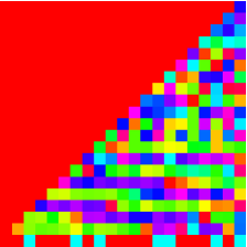
Each of these “noise” maps was added to each of the rotated Bianchi maps. We see from the example in Figure 6 that the spherical harmonic coefficients derived still have visible correlations in the phases for the Bianchi V map. The results of the Kolmogorov-Smirnov test (see Table 3) show that the correlations are still detectable and significant for the Bianchi V and VII_h maps but not so well for the VII₀ maps. So the method is better for detecting focused features that twisted features.

We see that the effect of adding fluctuations here is not dissimilar to adding just Gaussian noise. The concordance model predicts fluctuations which are stationary and Gaussian, as discussed in the Introduction (Section 1). Although these fluctuations are correlated on the sky, they have random phases so are incoherent with respect to what our statistic measures.

The “noise”, or fluctuation, maps are added to the Bianchi maps so that the ratio of the variances is of order unity. However, any ratio is possible; this specific choice is just for illustrative purposes to demonstrate the proposed methods. Nevertheless, if a random-phase (Gaussian) signal is superimposed on the Bianchi template, the phase coherence of the resulting map will still be degraded. If the Gaussian component is too large, the overall map will be indistinguishable from one with purely random phases.

In the examples we have shown, the Gaussian “noise” or fluctuation maps are added to the Bianchi maps in such a way that the ratio of the overall variance is of order unity. Our method still functions well with this level of “contamination”, but if the noise variance is much higher than that of the Bianchi maps the method begins to struggle.

So summarizing, the phases of the spherical harmonic coefficients are a very effective way of identifying focusing features in CMB maps, as long as the noise is not excessive, and can be used to give quantifiable significances. However, like the pixel distributions, the variation from the expectation of the concordance model only gives us an indication of non-Gaussianity. It is not clear in what form the non-Gaussianity occurs, such as an anisotropy or inhomogeneity. Hence the next section looks at multipole vectors which are built from spherical harmonic coefficients but can be used to give results in pixel (as opposed to harmonic) space, which is more meaningful from the point of view of diagnosing the presence of a preferred direction.

3.4 Application to WMAP 5 Year Data

For pedagogical interest, the methods described in Section 3.2 are applied here to the WMAP 5 year Internal Linear Combination (ILC) map. The results of the Kolmogorov-Smirnov test on the ILC map in the galactic coordinate system show very low significance correlations in $\Delta\Phi$ (see Table 4).

However Section 3.3 showed that to see the phase correlations, the Bianchi maps needed to be rotated close to the preferred axis. There have been studies that have found a preferred direction in the WMAP data, highlighted by the alignment of at least the quadrupole (${\ell}$ = 2) and octopole (${\ell}$ = 3). This preferred axis is known as the Axis of Evil. Therefore the methods from Section 3.2 are applied to the ILC map rotated so that the vertical axis aligns with the Axis of Evil. These $\Delta\Phi$ plotted in Figure 7 do not show any visual correlations. For comparison the figure also includes a plot of the same ILC data but with the phases replaced with random angles (i.e. so as to not affect the magnitude of the amplitudes of the $a_{l,m}$). Whilst the Kolmogorov-Smirnov test (Table 4) finds higher significance results than when the map was in Galactic coordinates, the results are still at a low significance.

The results show there is no significant detection, so if we do live in an anisotropic universe then it must be obscured with considerable “noise” (fluctuations). However the fact that the significance of the results do increase when the map is aligned with the Axis of Evil is intriguing.

Map	Axis	D	P(D) %
ILC	Galactic	0.06	66.20
ILC	Evil	0.07	86.05

Table 4: Results from the Kolmogorov-Smirnov test comparing the distribution of phase differences in the WMAP ILC map, rotated to align with either the galactic axis or axis of evil, with a random distribution of phase differences as predicted by the concordance model. D is the Kolmogorov-Smirnov statistic found when considering the phase differences. $P(\textbf{{D}})$ is the Monte Carlo estimate of the probability of getting the value of D, or less, found for the Bianchi models, from a random selection of phase differences. These are computed by forming an empirical distribution of D from sets of random simulations and counting what fraction of the ensemble gives the results obtained for the Bianchi maps. For example, in the case of the P(D) for the ILC map in the galactic plane we find that, out of 10000 simulations, 6620 have a value of D less than 0.06.

Figure 7: $\Delta\Phi$ for ${\ell}$, $m$ $\in$ [0, 20] for the ILC map with the Axis of Evil aligned with the preferred axis (left) and for the same map but with the phases replaced with random phases (right). Note that ${\ell}$ is plotted against the x axis, increasing from left to right, and $m$ is plotted against the y axis, increasing from bottom to top. No correlations are visible in either plot.

4 Multipole Vectors from Bianchi Universe

As shown in the previous section, the properties of spherical harmonic coefficients provide us with a generally effective way of identifying anisotropy through correlations in CMB maps. However the geometric interpretation of the mode correlations seen in harmonic space is by no means easy to interpret geometrically. In an effort to use the spherical harmonics to provide more meaningful explanation of non-Gaussianities found, we now consider an alternative approach, based on multipole vectors These can be constructed from spherical harmonics, using the $a_{{{\ell}m}}$ coefficients derived from CMB maps, but they give results in real (i.e. pixel) space. For a summary of the main terminology for the multipole vectors, using the polynomial interpretation approach which was introduced by Katz & Weeks (2004), please see Appendix A.

4.1 Results for Bianchi maps

Figure 8: The multipole vectors from Bianchi V map: dipole (left), quadrupole (middle) and octopole (right).

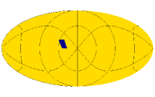
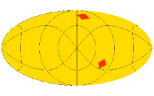
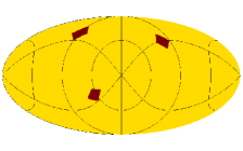
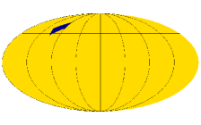
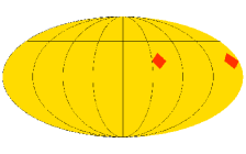
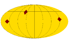
Figure 8 shows the multipole vectors from the Bianchi V map which serves as a good example to show how strongly the multipoles are correlated. The dipole (left) lies exactly at the top of the sphere, which is at the centre of the image. The two quadrupole vectors (middle) are located on the same spots on which two of octopole vectors (right) are placed. The remaining octopole vector is in the centre, i.e. the same place as dipole. Now we plot the dipole, quadrupole and octopole on the same 2-sphere for all the Bianchi maps, at different redshifts, to see how exactly they overlap (see Figure 9). The background colours indicate if any of the multipoles over-lap; yellow for no overlapped multipoles, green for overlapped dipole and octopole, light yellow for overlapped quadrupole and octopole, and light blue if all the multipole vectors are overlapped. The z-axis is into the page and the x-y plane is the large marked circle.

Figure 9: The multipole vectors from the Bianchi V (left), VII_h (middle) and VII₀ (right) maps from early stage (bottom panel) to late time (top panel). The vectors are represented by dots: dark blue for the dipole, light red for the quadrupole and brown for the octopole. Background colours also indicate if any of the multipoles over-lap; yellow for no overlapped multipoles (right column and bottom of middle column), green for overlapped dipole and octopole, light yellow (bottom of left column) for quadrupole and octopole and light blue (top of left column) if all the multipole vectors are overlapped.

First of all, in all types of the Bianchi models, we see the quadrupole and octopole vectors lie on the same plane, except for one of the octopole vectors which is always located in the centre of the image. For the Bianchi V and VII_h types, the dipole vectors lie very near the centre in the early stage but not exactly on it. However, as time goes on, the dipole vector is overlapped by one of the octopole vectors in the centre. The dipole vector of Bianchi VII₀ type is different from Bianchi VII_h. In the Bianchi VII₀ type, there is no particular correlation between the dipole and other multipoles since the dipole is not coupled with the other multipoles (quadrupole and octopole). For the Bianchi V (left), at the beginning of the stage, the dipole vector is ‘almost’ on the z-axis and one of octopole vectors is exactly on the z-axis. However the two later-time Bianchi V cases on the top left of Figure 9 show the dipole and octopole are on the same spot, in the middle of the image, which is exactly on the z-axis. Meanwhile, one of components of quadrupole and octopole vectors are on the same spot on the x-y plan. This means that the later Bianchi V models have more extreme correlation between the multipoles.

4.2 Results for WMAP Data

Again for pedagogical interest, the multipole vectors are applied to the WMAP 5 year Internal Linear Combination (ILC) map in Figure 10. At first glance, the results in the top row look like they might be clustered in a similar way to those in the Bianchi models (see Figure 9). However when we look at the results in the second row, where the map is orientated in the usual galactic coordinates, we see the multipoles line up along the x-y plane. This suggests an alternative explanation that the clustering near the x-y plane could be a feature of the residual galactic contamination which is known to remain in the full sky ILC maps.

Figure 10: The multipole vectors from the WMAP 5 year ILC map: dipole (left), quadrupole (middle) and octopole (right). The top row shows results where the z-axis is into the page and the x-y plane is the large marked circle. The bottom row shows results where the z-axis is the vertical line and the x-y plane is the horizontal line across the centre of the map.

5 Discussion and Conclusions

The aim of this article was to explore some simple ways of characterizing the large-scale temperature patterns in CMB maps generated in anisotropic Bianchi type V, VII_h and VII₀ universes. The ultimate purpose of investigating this behavior is to find ways of quantifying the global properties of the pattern produced in order to isolate the effect of anisotropy from that of non-Gaussianity. We repeat that when we talk about non-Gaussianity here is not related to a stochastic field; there are no fluctuations in the Bianchi maps.

We first discussed perhaps the simplest and perhaps the most obvious possible descriptive statistics, the histogram of the pixel values, primarily with the aim of demonstrating how non-Gaussianity of a sort can arise from asymmetry. We evaluated the pixel distribution functions for each of the maps and compared them to results expected in a universe consistent with the concordance model. The type VII₀ maps show the strongest deviation from the null hypothesis; but types V and VII_h behaved in a similar fashion to each other, and closer to that of the null hypothesis. The reason these two gave lesser indications of the presence of anomalies was because the focussing effect produces a pattern that covers only a smaller part of the celestial sphere, which tends to get lost when averaged over the whole sky. This method is therefore useful to characterize coherent signals extended over a large region, such as a spiral pattern, but not if they are concentrated.

Phase analysis is a relatively new technique, and has consequently not been used to quantify many alternative situations to the concordance model. The phases of the spherical harmonic coefficients provide a generic way of looking at correlations in harmonic space that could arise from non-stationarity or non-Gaussianity. While this is a potential strength of the approach - while phase correlations will not just be useful for identifying anisotropies specific to the Bianchi models, but in theory any isotropy introduced to the CMB - it could also prove a weakness, in that more general methods may lack the power to discriminate very specific models.

The phase correlations identified in our Bianchi maps using this technique were much stronger than we at first expected; given the generic nature of the metric it was not expected to yield good results. In addition to this, the strong correlations were found to be robust to both rotation and moderate noise. Significant correlations in both twisted and focusing features were also identified. However using the same methods on the WMAP 5 year data shows little evidence of non-Gaussianity. Given that the diagnostics are identified in harmonic space, it is difficult to say whether any of the anomalies identified this way are down to isotropy or homogeneity.

The analysis of multipole vectors is also a relatively new technique. It has been used to identify non-Gaussianities in the WMAP data, and has been particularly successful in identifying anisotropies (i.e. asymmetries and/or preferred directions). The multipole vectors are calculated from spherical harmonic coefficients which, as we have already shown, themselves provide a very effective way of identifying correlations in Bianchi (and presumably other anisotropic) patterns. The multipole vectors must include at least some of the information needed to describe these mode correlations. The advantage of multipole vectors over the spherical harmonics themselves, however, is that they give results in real (i.e. pixel) space which is much more informative to the user. The results when applied to the Bianchi maps show very strong correlations between the directions of the multipole vectors for low ${\ell}$, often with them entirely overlapping, and hence showing preferred directions. Since these vectors would not be aligned in the case of a stationary stochastic field over the sky, these results demonstrate that they are sensitive to departures from the standard cosmological model.

It remains the case that the standard cosmological model is a good fit to a huge range of observational data. Nevertheless, it is important that tools are developed that are sufficiently sensitive to hunt efficiently for possible anomalies in the next generation of observations. There are many ways that the CMB temperature pattern could be anomalous other than through the presence of Bianchi perturbation modes such as those we have studied here. Just as there are many ways a distribution can be non-Gaussian, so are there also many ways a fluctuation field can be non-stationary. Testing for departures from the standard model will require not one but a battery of statistical techniques each sensitive to particular aspects of the distribution.

This has been a very preliminary analysis, aimed at establishing whether the diagnostics described in this paper are in principle capable of uncovering evidence of underlying anomalies in CMB data. Of course these patterns represent somewhat extreme departures from the standard framework so it is no real surprise that they register strongly in the descriptors used. However, in all cases our analysis has involved only a relatively small number of quantities, so the fact that we see quantifiable effects emerging is very encouraging.

Appendix A Multipole vectors terminology

Any homogeneous polynomial $F_{R}$ of degree ${\ell}$ in $x$, $y$ and $z$ can be written as

$$F_{R}(x,y,z)=\lambda\cdot(a_{1}x+b_{1}y+c_{1}z)\cdot(a_{2}x+b_{2}y+c_{2}z)\cdots(a_{\ell}x+b_{\ell}y+c_{\ell}z)+S_{R}\cdot G_{R}.$$ (4)

The function $G_{R}$ is homogeneous of degree ${\ell}-2$ and $S_{R}=x^{2}+y^{2}+z^{2}$. All polynomials $F_{R}$, $G_{R}$ and $S_{R}$ and all variables are real. If we consider the values taken by the polynomial on the unit sphere where $S_{R}=x^{2}+y^{2}+z^{2}=1$ then the above expression reduces to the product of the linear parts together with the term $G_{R}$. This can be extended to a complex polynomial through

$$F(x,y,z)=\lambda L_{1}L_{2}\cdots L_{\ell}+S\cdot G$$ (5)

where $L_{i}=a_{i}x+b_{i}y+c_{i}z$ and $x$, $y$ and $z$ are complex numbers, while the coefficients of $F$ ($a_{i},b_{i},c_{i},$ and $\lambda$) are real. $G$ is a homogeneous polynomial of degree ${\ell}-2$ and $S$ is given by $x^{2}+y^{2}+z^{2}$. We are interested in the value of the polynomial $F$ on the 2-sphere which, in the complex space, takes the form $S=x^{2}+y^{2}+z^{2}=0$. By Bézout’s theorem, which holds that the number of points on two curves is equal to the product of their degrees, there are 2${\ell}$ points in which the complex curve $F(x,y,z)=0$ intersects the quadratic curve $S(x,y,z)=0$, which is topologically a 2-sphere. Since the complex curve $F=0$ intersects the complex $S=0$ in 2${\ell}$ points, the product curves $L_{i}$ also intersect $S=0$ in the same 2${\ell}$ points, $f_{i}=(x_{i},y_{i},z_{i})$. Moreover, its complex conjugate $f^{*}_{i}=(x^{*}_{i},y^{*}_{i},z^{*}_{i})$ has to lie in the intersection in which both $F$ and $S$ are zero. We thus obtain the 2${\ell}$ points of intersection $\{f_{1},f^{*}_{1},\cdots,f_{\ell},f^{*}_{\ell}\}$.

Each pair $\{f_{\ell},f^{*}_{\ell}\}$ determines a unique line $L_{i}=a_{i}x+b_{i}y+c_{i}z=0$ with real coefficients such that:

$$a_{i}x^{Re}_{i}+b_{i}y^{Re}_{i}+c_{i}z^{Re}_{i} = 0$$

$$a_{i}x^{Im}_{i}+b_{i}y^{Im}_{i}+c_{i}z^{Im}_{i} = 0$$ (6)

where the coefficients are normalized to unit length, i.e. $a^{2}_{i}+b^{2}_{i}+c^{2}_{i}=1$. Note that the index $i$ has no sum and $1\leq i\leq{\ell}$. In order to find the multipole vectors, $v_{i}=(a_{i},b_{i},c_{i})$, of each ${\ell}$ we need to find the pairs of $f_{i}$ which lie on the curve $F=0$ and $S=0$ in the complex projective plane i.e. finding the roots ($\alpha$) which satisfy $F=0$ on the 2-sphere ($S=0$). What is required is to factorize the homogeneous, harmonic polynomial, $F$ into linear factors i.e. such that $F$ is the product of $L_{i}$ only. However, this is not possible analytically since they are not linear equations far from the dipole. Fortunately, the curve $S=0$ can be parametrized as a single variable and the polynomial $F$ as:

$$F(x,y,z)=F(i(\alpha^{2}-1),-2i\alpha,\alpha^{2}+1).$$ (7)

From Equation 7, the roots $\alpha$ which satisfy $F=0$ and $S=0$, or the product of $L_{i}$=0, can be found. Once the roots $\alpha$ are found, the pair of $\{f_{i},f^{*}_{i}\}$ can be expressed in terms of x, y and z. The next step is to find the multipole vectors from Equation A by using $f_{i}=(x^{Re},y^{Re},z^{Re})+i(x^{Im},y^{Im},z^{Im})$ or its conjugate $f^{*}_{i}$ since the two points give same result.

We now apply this terminology to the relevant cosmological application, that of temperature patterns on the CMB sky, as follows. The ${\ell}^{th}$ multipoles, $T_{\ell}$, can be represented by a polynomial $F$ on the 2-sphere ($S=0$), or the product of $L_{i}$. By the given relations $x=i(\alpha^{2}-1)$, $y=-2i\alpha$, and $z=\alpha^{2}+1$, the spherical harmonics can be expanded as $\alpha$ terms. Thus the dipole ($T_{1}$), quadrupole ($T_{2}$) and octopole ($T_{3}$) can be described in terms of $\alpha$ with the $a_{{{\ell}m}}$ as coefficients. The $a_{{{\ell}m}}$ were calculated using Healpix from the maps, and we found the roots $\alpha$ which satisfy equations $T_{\ell}$=0 for each ${\ell}$. These roots gave a pair of $\{f_{\ell},f^{*}_{\ell}\}$ , therefore from Equation A we obtained solution sets $v_{i}=(a_{i},b_{i},c_{i})$ which are multipole vectors for each ${\ell}$.

We now explain this procedure in detail for each of the multipoles considered:

A.0.1 Dipole: ${\ell}=1$.

$$T_{1} = \sum_{m}a_{1m}Y_{1m}$$ (8)

$$= \sqrt{\frac{3}{2\pi}}(a^{Re}_{11}x-a^{Im}_{11}y+\frac{a_{10}}{\sqrt{2}}z)$$ (9)

For the dipole vector it is not necessary to use the $\alpha$ notation since it is a linear equation in $x$, $y$ and $z$. In our polynomial notation, the dipole is also represented as

$$F=L_{1}=\lambda_{1}(a_{1}x+b_{1}y+c_{1}z).$$ (10)

From the normalization, we obtain the multipole vector,

$$v_{1}=(\sqrt{\frac{2}{3C_{1}}}a^{Re}_{11},-\sqrt{\frac{2}{3C_{1}}}a^{Im}_{11},\frac{1}{\sqrt{3C_{1}}}a_{10}),$$ (11)

and the coefficient,

$$\lambda_{1}=\sqrt{\frac{3}{2\pi}}\sqrt{a^{2Re}_{11}+a^{2Im}_{11}+\frac{1}{2}a^{2}_{10}}=\sqrt{\frac{3}{2\pi}}\sqrt{a^{2}_{11}+\frac{1}{2}a^{2}_{10}}=\frac{3}{2}\sqrt{\frac{C_{1}}{\pi}}$$ (12)

where the C${}_{1}=(2|a_{11}|^{2}+a^{2}_{10})/3$ is the angular power spectrum C_ℓ of the monopole.

A.0.2 Quadrupole: ${\ell}=2$.

In this case we need to expand $T_{2}$ using the $\alpha$ notation since for multipoles from the quadrupole to higher order the equations are no longer linear. The quadrupole on the sphere has two multipole vectors, $\upsilon_{1}$ and $\upsilon_{2}$, from $F=L_{1}L_{2}=\lambda_{1}(a_{1}x+b_{1}y+c_{1}z)(a_{2}x+b_{2}y+c_{2}z)$. In order to find them, we transfer the quadrupole expression from spherical harmonics to $\alpha$ notation for efficient computing,

$$T_{2} = \sum_{m}a_{2m}Y_{2m}$$ (14)

$$= (\sqrt{\frac{3}{2}}a_{20}-a^{Re}_{22}+2ia^{Re}_{21})\alpha^{4}-4(a^{Im}_{22}-ia^{Im}_{21})\alpha^{3}+(\sqrt{6}a_{20}+6a^{Re}_{22})\alpha^{2}$$

$$\quad+4(a^{Im}_{22}+ia^{Im}_{21})\alpha+\sqrt{\frac{3}{2}}a_{20}-a^{Re}_{22}-2ia^{Re}_{21}$$

A.0.3 Octopole: ${\ell}=3$.

We use the same method as we have done for the quadrupole. The octopole has three multipole vectors, $\upsilon_{1}$, $\upsilon_{2}$ and $\upsilon_{3}$, from $F=L_{1}L_{2}L_{3}=\lambda_{1}(a_{1}x+b_{1}y+c_{1}z)(a_{2}x+b_{2}y+c_{2}z)(a_{3}x+b_{3}y+c_{3}z)$, which gives a $6^{th}$ order of equation in $\alpha$:

$$T_{3} = \sum_{m}a_{3m}Y_{3m}$$ (15)

$$= A_{6}\alpha^{6}+A_{5}\alpha^{5}+A_{4}\alpha^{4}+A_{3}\alpha^{3}+A_{2}\alpha^{2}+A_{1}\alpha+A_{0},$$ (16)

in which the coefficients are,

$$A_{6} = 5a_{30}-\sqrt{30}a^{Re}_{32}+(-5\sqrt{3}a^{Re}_{31}+\sqrt{5}a^{Re}_{33})i$$

$$A_{5} = -4\sqrt{30}a^{Im}_{32}+(-10\sqrt{3}a^{Im}_{31}+6\sqrt{5}a^{Im}_{33})i]$$

$$A_{4} = 5[3a_{30}+\sqrt{30}a^{Re}_{32}-(\sqrt{3}a^{Re}_{31}+3\sqrt{5}a^{Re}_{33})i$$

$$A_{3} = -20(\sqrt{3}a^{Im}_{31}+\sqrt{5}a^{Im}_{33})i$$

$$A_{2} = A_{4}^{*},A_{1}=-A_{5}^{*},A_{0}=A_{6}^{*}.$$

Each multipole has 2${\ell}$ roots of $\alpha$ which gives the $(f_{i},f^{*}_{i})$ pairs, however only ${\ell}$ components are used to find the multipoles since their conjugators give the same results, as we mentioned earlier.

References

- Abramo et al. (2006) Abramo L. R., Bernui A., Ferreira I. S., Villela T., Wuensche C. A., 2006, Phys. Rev. D, 74, 063506
- Bardeen, Steinhardt & Turner (1983) Bardeen J. M., Steinhardt P. J., Turner M. S., 1983, Phys. Rev. D, 28, 679
- Barrow, Juszkiewicz & Sonoda (1985) Barrow J. D., Juszkiewicz R., Sonoda D. H., 1985, MNRAS, 213, 917
- Bennett et al. (2003) Bennett C. L. et al., 2003, ApJS, 148, 1
- Bielewicz et al. (2005) Bielewicz P., Eriksen H. K., Banday A. J., Górski K. M., Lilje P. B., 2005, ApJ, 635, 750
- Bielewicz & Riazuelo (2009) Bielewicz P., Riazuelo A., 2009, MNRAS, 396, 609
- Bridges et al. (2008) Bridges M., McEwen J.D., Cruz M., Hobson M.P., Lasenby A.N., Vielva P., Martínez-Gonzalez E., 2008, MNRAS, 390, 1372
- Bunn, Ferreira & Silk (1996) Bunn E. F., Ferreira P., Silk J., 1996, Phys. Rev. Lett., 635, 750
- Chiang, Naselsky & Coles (2004) Chiang L.-Y., Naselsky P. D., Coles P., 2004, ApJ, 602,L1
- Chiang et al. (2007) Chiang L.-Y., Coles P., Naselsky P. D., Olesen P., 2007, JCAP, 1, 21
- Chiang, Naselsky & Coles (2007) Chiang L.-Y., Naselsky P. D., Coles P., 2007, ApJ, 664, 8
- Coles et al. (2004) Coles P., Dineen P., Earl J., Wright D., 2004, MNRAS, 350, 989
- Coles & Chiang (2000) Coles P., Chiang L.-Y., 2000, Nat, 406, 376
- Copi, Huterer & Starkman (2004) Copi C. J. , Huterer D., Starkman G. D., 2004, Phys. Rev. D, 70, 043515
- Copi et al. (2006) Copi C. J. , Huterer D., Schwarz D. J., Starkman G. D., 2006, MNRAS, 367, 79
- Copi et al. (2007) Copi C. J. , Huterer D., Schwarz D. J., Starkman G. D., 2007, Phys. Rev. D., 75, 023507
- Cruz et al. (2005) Cruz M., Martínez-González E., Vielva P., Cayón L., 2005, MNRAS, 356, 29
- Dineen, Rocha & Coles (2005) Dineen P., Rocha G., Coles P., 2005, MNRAS, 358, 1285
- Ellis & MacCallum (1969) Ellis G. F. R., MacCallum M. A. H., 1969, Commun. Math. Phys., 12, 108
- Eriksen et al. (2004) Eriksen H. K., Hansen F. K., Banday A. J., Górski K. M., Lilje P. B., 2004, ApJ, 605, 14
- Eriksen et al. (2005) Eriksen H. K. et al., 2005, astro-ph/0508196
- Eriksen et al. (2007) Eriksen H. K., Banday A. J., Górski K. M., Hansen F. K., Lilje P. B., 2007, ApJ, 660, L81
- Górski et al. (2005) Górski K. M., Hivon E., Banday A. J., Wandelt B. D., Hansen F. K., Reinecke M., Bartelmann M., 2005, ApJ, 622, 759
- Guth & Pi (1982) Guth A. H., Pi S. Y., 1982, Phys. Rev. Lett., 49, 1110
- Hansen et al. (2009) Hansen F. K., Banday A. J., Górski K. M., Eriksen H. K., Lilje P. B., 2009, ApJ, 704, 1448
- Hinshaw et al. (2009) Hinshaw G. et al., 2009, ApJS, 180, 225
- Hoftuft et al. (2009) Hoftuft J., Eriksen H. K., Banday A. J., Górski K. M., Hansen F. K., Lilje P. B., 2009, ApJS, 699, 985
- Jaffe et al. (2005) Jaffe T. R., Banday A. J., Eriksen H. K., Górski K. M., Hansen F. K., 2005, ApJ, 629, L1
- Jaffe et al. (2006a) Jaffe T. R., Banday A. J., Eriksen H. K., Górski K. M., Hansen F. K., 2006, ApJ, 643, 616
- Jaffe et al. (2006b) Jaffe T. R., Banday A. J., Eriksen H. K., Górski K. M., Hansen F. K., 2006, A&A, 640, 393
- Katz & Weeks (2004) Katz G., Weeks J., 2004, Phys. Rev. D, 70, 063527
- Kogut, Hinshaw & Banday (1997) Kogut A., Hinshaw G., Banday A. J., 1997, Phys. Rev. D, 55, 1901
- Land & Magueijo (2005a) Land K., Magueijo J., 2005a, MNRAS, 357, 994
- Land & Magueijo (2005b) Land K., Magueijo J., 2005b, MNRAS, 362, L16
- Land & Magueijo (2005c) Land K., Magueijo J., 2005c, Phys. Rev. D, 72, 101302(R)
- Land & Magueijo (2005d) Land K., Magueijo J., 2005d, Phys. Rev. Lett., 95, 071301
- Land & Magueijo (2005e) Land K., Magueijo J., 2005e, MNRAS, 362, 838
- Land & Magueijo (2007) Land K., Magueijo J., 2007, MNRAS, 378, 153
- McEwen et al. (2006) McEwen J. D., Hobson M. P., Lasenby A. N., Mortlock D.J., 2006, MNRAS, 369, 1858
- Maxwell (1891) Maxwell J. C., A Treatise on Electricity and Magnetism (Clarendon Press, London, 1891), Vol. I, 3rd edition.
- Park (2004) Park C., 2004, MNRAS, 349, 313
- Pontzen (2009) Pontzen A., 2009, Phys. Rev. D., 79, 103518
- Pontzen & Challinor (2007) Pontzen A., Challinor A., 2007, MNRAS, 380, 1387
- Schwarz et al. (2004) Schwarz D. J., Starkman G. D., Huterer D., Copi C. J., 2004, Phys. Rev. Lett., 93, 221301
- Stannard & Coles (2005) Stannard A., Coles P., 2005, MNRAS, 364, 929
- Starobinskij (1982) Starobinskij A. A., 1982, Phys. Lett. B, 117, 175
- Sung & Coles (2009) Sung R., Coles P., 2009, CQGra, 26, 172001
- Sung & Coles (2010) Sung R., Coles P., 2010, JCAP, submitted, arXiv:1004.0957 (astro-ph.CO)
- Vielva et al. (2004) Vielva P., Martínez-González E., Barreiro R. B., Sanz J. L., Cayón L., 2004, ApJ, 609, 22
- Yadav & Wandelt (2008) Yadav A. P. S., Wandelt B. D., 2008, Phys. Rev. Lett., 100, 181301