Spatiotemporal correlations of aftershock sequences

Abstract

Aftershock sequences are of particular interest in seismic research since they may condition seismic activity in a given region over long time spans. While they are typically identified with periods of enhanced seismic activity after a large earthquake as characterized by the Omori law, our knowledge of the spatiotemporal correlations between events in an aftershock sequence is limited. Here, we study the spatiotemporal correlations of two aftershock sequences form California (Parkfield and Hector Mine) using the recently introduced concept of “recurrent” events. We find that both sequences have very similar properties and that most of them are captured by the space-time epidemic-type aftershock sequence (ETAS) model if one takes into account catalog incompleteness. However, the stochastic model does not capture the spatiotemporal correlations leading to the observed structure of seismicity on small spatial scales.

PEIXOTO ET AL. SPATIOTEMPORAL CORRELATIONS OF AFTERSHOCK SEQUENCES

1 Introduction

One of the grand challenges for seismology is to establish the relationship between stress and strain in the lithosphere (Forsyth et al., 2009). While motions of tectonic plates and surface deformations can be measured precisely with satellite imaging and networks of Global Positioning System receivers, strainmeters, seismometers and tiltmeters, the causative stress can only be inferred. However, the temporally and spatially dependent rheology which describes the linkage between the forces (stresses) and the resulting deformations (strains) is generally not well understood (Kanamori and Brodsky, 2004). This makes it currently impossible to conclusively answer how some earthquakes trigger other earthquakes thousands of kilometers away, for example, and to predict earthquakes reliably.

An alternative approach to gain insight into the underlying dynamics of earthquakes is to study the spatiotemporal patterns of seismicity where each earthquakes is treated as a point event in space and time with a given magnitude. Such an approach may shed light on the fundamental physics since these patterns are emergent processes of the underlying many-body nonlinear system. Indeed, it has been proved successful in many cases and led to the discovery of new key features of seismicity (Rundle et al., 2003; Corral, 2004; Davidsen and Goltz, 2004; Shcherbakov et al., 2004; Davidsen and Paczuski, 2005; Baiesi and Paczuski, 2005; Felzer and Brodsky, 2006; Hainzl et al., 2006; Corral, 2006; Marsan and Lengliné, 2008; Zaliapin et al., 2008). For example, in Davidsen et al. (2006, 2008) the spatiotemporal clustering of earthquakes in Southern California was found to show non-trivial features which led to a new and independent estimate of the rupture length and its scaling with magnitude. In particular, the results provide further evidence for a shadowing effect associated with smaller earthquakes (Rubin, 2002; Fischer and Horálek, 2005; Hainzl and Marsan, 2008). The key to these findings was a unique approach to quantify non-trivial spatiotemporal clustering based on the view that any suitable definition of clustering should be purely contextual and depend only on the actual history of events without any further assumptions (Davidsen et al., 2008). This approach utilizes the notion of space-time records to define “recurrences” and maps seismicity onto a graph or network, thus, allowing the characterization of spatiotemporal clustering by means of tools from complex network theory (Albert and Barabasi, 2002; Newman, 2003).

To elucidate the origin of the observed non-trivial clustering further, we study here the spatiotemporal correlations of aftershock sequences which follow large shallow earthquakes. Aftershocks are the most obvious example of earthquakes that are triggered in part by preceding events as follows from the observed increased seismic activity captured by the Omori law (Utsu et al., 1995). Thus, their specific clustering in space and time should provide information on the underlying dynamics and triggering mechanisms — see, for example, (Felzer and Brodsky, 2006; Gomberg and Felzer, 2008). Moreover, aftershocks are important from a conceptual point of view since the current main paradigm in statistical seismology classifies earthquakes as triggered events like aftershocks and “background” events which are hypothesized to be induced by other means. It is important to realize, however, that the notion of background events — and aftershocks, for that matter — is not well-defined as no clear physical difference between such events has been established. In particular, background events could be artifacts to a large extent since small earthquakes can trigger larger events (Helmstetter et al., 2006; Marsan and Lengliné, 2008) and many small earthquakes are typically not detected (Sornette and Werner, 2005a, b).

For the aftershock sequences associated with the Parkfield earthquake (September 28, 2004) and the Hector Mine earthquake (October 16, 1999), we find that both sequences show very similar spatiotemporal correlations as quantified by the method of Davidsen et al. (2006, 2008). While most features are also similar to what has been observed previously for a 20-year catalog from Southern California (Davidsen et al., 2008), there is no indication of a shadowing effect. Moreover, we find that most of the observed features can be captured by a space-time version of the epidemic-type aftershock sequence (ETAS) model (Helmstetter and Sornette, 2002a; Ogata and Zhuang, 2006) if catalog incompleteness (Lennartz et al., 2008a) is taken into account. This suggests that the spatiotemporal correlations are to a large extent a consequence of a few established laws of seismicity and missing data. This was further confirmed by a comparison with a simple non-homogeneous Poisson (NHP) model following the Omori law, but without any spatiotemporal correlations between events. Yet, we find that this stochastic model has several shortcomings with respect to the spatial distribution of seismicity.

2 Aftershock sequences and the ETAS model

Although there is considerable statistical variability associated with aftershocks, their behavior appears to satisfy several scaling laws to a reasonably good approximation. Among them are the Gutenberg-Richter scaling relation for the frequency-magnitude distribution (Gutenberg and Richter, 1949) which is certainly satisfied on long time scales (Shcherbakov et al., 2006), Båth’s law for the difference between the magnitudes of a mainshock and its largest aftershock (Båth, 1965) as well as the modified Omori law for the temporal decay of aftershock rates (Utsu et al., 1995; Shcherbakov et al., 2004; Hainzl and Marsan, 2008; Narteau et al., 2009). More recently, another scaling law characterizing the epicenter distribution of aftershocks has been found (Felzer and Brodsky, 2006).

In an attempt to establish a statistical null model of aftershocks which would incorporate some of these scaling laws, the epidemic-type aftershock sequence (ETAS) model was introduced (Kagan and Knopoff, 1987; Ogata, 1988; Helmstetter and Sornette, 2002b). This model describes a stochastic branching process in which any earthquake may trigger other earthquakes, which in turn may trigger more, and so on. In particular, the location and the time of occurrence of each “daughter” event is strongly correlated to its “mother” event: The occurrence rate of daughter events at time $t$ and position $\vec{r}$ triggered by a mother event of magnitude $m_{i}$, at time $t_{i}$ and position $\vec{r}_{i}$, is defined as

$$\phi_{m_{i}}(t-t_{i},\vec{r}-\vec{r}_{i})=\rho(m_{i})\Psi(t-t_{i})\Phi_{m_{i}}(\vec{r}-\vec{r}_{i}),$$ (1)

where $\rho(m_{i})$ is the average number of aftershocks directly triggered by an event of magnitude $m_{i}$, $\Psi(t-t_{i})$ is the normalized temporal distribution of directly triggered events and $\Phi_{m_{i}}(\vec{r}-\vec{r}_{i})$ is the normalized spatial distribution of directly triggered events in two dimensions. $\rho(m_{i})$ is assumed to follow the productivity law

$$\rho(m_{i})=K10^{\alpha(m_{i}-m_{0})},$$ (2)

where $m_{i}>m_{0}$ and $K$, $\alpha$ are constants. Note that the productivity law is zero below $m_{0}$ implying that events smaller than $m_{0}$ do not trigger other earthquakes. This condition is necessary to ensure a finite total occurrence rate — see (Sornette and Werner, 2005a) for a discussion of its physical relevance. $\Psi(t)$ is assumed to be determined by the modified Omori law which can be written as

$$\Psi(t)=\frac{\theta c^{\theta}}{(t+c)^{1+\theta}}H(t),$$ (3)

where $c$, $\theta>0$ and $H(t)$ is the Heaviside step function. Note that the exponent $1+\theta$, which describes the time distribution of the direct aftershocks, is typically larger than the observed Omori exponent, which characterizes the whole cascade of directly and indirectly triggered aftershocks (Helmstetter and Sornette, 2002b; Marsan and Lengliné, 2008). Finally, $\Phi_{m}(\vec{r})$ is assumed to follow the recently established epicenter distribution of aftershocks (Helmstetter and Sornette, 2002b; Felzer and Brodsky, 2006) which can be expressed as

$$\Phi_{m}(\vec{r})=\frac{\mu}{d(m)\left(|\vec{r}|/d(m)+1\right)^{1+\mu}},$$ (4)

where $\mu=0.35$ and $d(m)=d_{0}10^{0.45m}$ with $d_{0}=15$m is the rupture length of the triggering event of magnitude $m$ (Wells and Coppersmith, 1994; Kagan, 2002; Davidsen et al., 2008). Note that this expression is already problematic since it assumes a rotationally symmetric distribution of aftershocks, thus, neglecting the typically anisotropic fault structure on which aftershocks occur and also neglecting the frequent observation that the mother event is located on the margin of the area of triggered events. Since the epicenters of the aftershock sequences considered here are approximately located on a single fault, we focus on the one-dimensional case and discuss the two-dimensional case as necessary.

The magnitude $m_{i}$ of each event is independently sampled from the normalized Gutenberg-Richter distribution,

$$P(m)=b\ln(10)10^{-b(m-m_{0})},$$ (5)

where the constant $b$ is typically close to 1 and $m_{0}$ is again the lower threshold, below which no aftershocks are initiated.

An important quantity in the ETAS model is the average number of $n$ of daughter events per earthquake, averaged over all magnitudes, which is given by

$$n =\int d\vec{r}\int_{t_{i}}^{\infty}dt\int_{m_{0}}^{\infty}dm_{i}P(m_{i})\phi_{m_{i}}(t-t_{i},\vec{r}-\vec{r_{i}})$$ (6)

$$=\frac{Kb}{b-\alpha},$$ (7)

where the last equation assumes $\alpha<b$ which has been suggested as the relevant regime (Marsan and Lengliné, 2008).

2.1 Data sets and parameter values

Here, we study the aftershock sequences associated with the Parkfield earthquake ($M=6.0$, September 28, 2004) and the Hector Mine earthquake ($M=7.1$, October 16, 1999) as identified in Shcherbakov et al. (2004, 2006). In both cases, the high-quality seismic network in the vicinity of these mainshocks provided a particularly well-documented sequence of aftershocks. This is especially true for the Parkfield sequence (Bakun et al., 2005). For Parkfield, the number of identified aftershock over a time period of $T=365$ days is $2056$ above magnitude $m=1.15$. For Hector mine, we have $5380$ aftershocks above $m=2.0$. Both aftershock sequences differ significantly in their spatial extent and also slightly in the exponents of the Omori law and the Gutenberg-Richter law.

In principle, it seems straightforward to estimate the parameters of the ETAS model for a given aftershock sequence. Yet, an important aspect of any aftershock sequence is that at early times after a mainshock not all (small) aftershocks are detected due to the large amount of seismic noise (Kagan, 2004; Kagan and Houston, 2005; Peng et al., 2006). This has led to the proposition of a time-dependent magnitude threshold of completeness which involves further parameters (Helmstetter et al., 2006). To take this into account, we proceed as follows: First we generate artificial aftershock sequence from the ETAS model for a given main event with magnitude $M$ as outlined in the Appendix .1. Then, we impose two constraints on the generated catalog to take into account the finite area size covered by the empirical catalogs and to mimic missing data: i) events that lie outside of the spatial area considered for the empirical catalogs were discarded; ii) events below the time-varying magnitude threshold of completeness $m_{c}(M,t)$ were discarded with a certain probability according to the procedure described in Lennartz et al. (2008b). To be more precise, we define $m_{C}(M,t)=\max{[m_{1}(M,t),m_{2}]}$ where $m_{1}(M,t)=M-4.5-0.75\log_{10}(t)$ reflects the incompleteness at time $t$ after the main event of magnitude $M$, and the time-independent sensitivity of the seismic network, different for each empirical catalog, is captured by the constant $m_{2}$. Then, the probability of observing an event of magnitude smaller than the threshold $m_{c}(M,t)$ is given by $p_{j}(m)=10^{-\gamma_{j}(m_{j}-m)}$, where $j=1$ if $m_{C}(M,t)=m_{1}(M,t)$ and $j=2$ otherwise.

Using the parameters estimated in Lennartz et al. (2008a) for the Parkfield and Hector mine aftershock sequences, only $K$ and $\alpha$ of the ETAS model as well as the fraction of background events have to be approximated. Our selection criteria were both the total number of events in the catalogs, and the functional form of the total event rate (see Eq. (8)). The background rate was set at $1$ event/day, which gives a total event rate in very good agreement with the empirical data (not shown). The other two parameters were chosen, such that the average catalog size was similar to the empirical catalogs (after some events were discarded by the procedure outlined above), i.e., $2056$ for Parkfield and $5380$ for Hector Mine, with an accepted deviation of at most $\pm 200$ events per catalog. In total, $100$ artificial Parkfield and Hector Mine catalogs were generated. The parameter values used for simulating the two different aftershock sequences are summarized in table 1.

Event	$M$	$m_{0}$	$\theta$	$c$ (days)	$b$	$\alpha$	K	$\gamma_{1}$	$m_{2}$	$\gamma_{2}$	$\lambda_{b}$ (days-1)
Parkfield	$6.0$	$1.15$	$0.09$	$0.00395$	$0.89$	0.8	0.2	$0.7$	$1.2$	$1.5$	1
Hector Mine	$7.1$	$2.0$	$0.21$	$0.024$	$1.01$	0.789	0.28	$1.8$	$1.4$	$1.5$	1

Table 1: Parameters used for the ETAS model.

3 Network of recurrences

We analyze the two aftershock sequences and the catalogs generated by the ETAS model according to a recently proposed method which allows one to characterize the spatiotemporal clustering of seismicity (Davidsen et al., 2006, 2008). It is based on the notion of a recurrence in the context of spatiotemporal point processes: An event is defined to be a recurrence of a given previous event if it occurs closer in space to that event than all intervening events. Recurrences are therefore record breaking events with respect to distance. This relationship is naturally represented by a directed network of recurrences: Each event $a_{k}$ defined by its location $\vec{r}_{k}$ and time of occurrence $t_{k}$, with $k=1,...,N$, is a vertex in the network and a directed edge from $a_{k}$ to $a_{m}$ exists for $k<m$ if $a_{m}$ is a recurrence of $a_{k}$, i.e., if the distance $|\vec{r}_{m}-\vec{r}_{k}|$ is smaller than the distance $|\vec{r}_{k^{\prime}}-\vec{r}_{k}|$ for all events $a_{k^{\prime}}$ with $k<k^{\prime}<m$. This definition assumes that the events are ordered according to their occurrence in time. Each recurrence, i.e. each edge on the network, is therefore characterized by the time interval $t=t_{m}-t_{k}$ between the two connected events $k$ and $m$ and analogously by the spatial distance $l$ between the two. Note that the mapping of the point process dynamics to the recurrence network is entirely data-driven and does not impose any arbitrary space and time scales other than those associated with the given event catalog.

To investigate the dependence of the network properties on the magnitude thresholds of events considered, we analyze networks obtained for different magnitude thresholds. This is crucial to identify robust features as well as potential scaling properties.

4 Results

4.1 Topological characteristics of the network

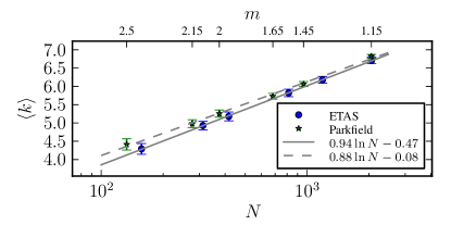
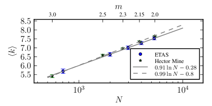
We turn now to the analysis of the statistical properties of the network of recurrences which have been proved useful in the analysis of the overall seismic activity in Southern California (Davidsen et al., 2006, 2008). The growth of the network can be measured by the average degree $\left<k\right>$ as a function of the number of events $N$ in the catalog. The in(out)-degree of a node is the number of edges pointing towards (away from) it and the in- and out-degree averaged over the entire network are obviously the same. The number of nodes $N$ can be controlled by changing the magnitude threshold above which events are considered for constructing the network. As can be seen in Fig. 1, the ETAS datasets as well as the empirical catalogs show a logarithmic increase of $\left<k\right>$ with $N$. Both for Parkfield and Hector Mine, the increase is compatible with the ETAS data sets if one takes into account the statistical uncertainties. In all cases, the behaviour is similar to what is expected if events were randomly, independently and uniformly placed in space and time, which would imply that the growth should follow $\left<k\right>\sim\ln N$ for large $N$ (Davidsen et al., 2008). Actually, this result even holds if the events are not uniformly distributed in time including the case of a simple non-homogeneous Poisson (NHP) model following the Omori law which by construction does not have any spatiotemporal correlations between events. The comparison with such a model is particularly helpful to identify statistical properties of the empirical aftershock series and of series generated by the ETAS model that arise trivially and are, thus, not due to spatiotemporal correlations. The properties of the NHP model are analytically derived and discussed in the Appendix .2.

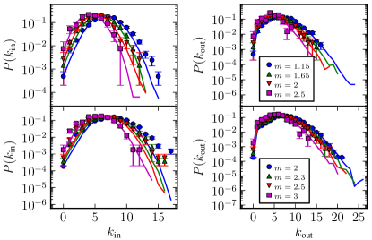
The probability distributions of in- and out-degrees can be seen in Fig 2. The out-degree distributions for both empirical and ETAS catalogs are in excellent agreement. While the distributions are compatible with a Poisson distribution over the range where we have non-zero values for the respective empirical catalog, the decay in the distribution for the respective ETAS catalog for larger values of $k_{out}$ is slightly but significantly slower than a Poisson distribution (not shown). The reason that we actually observe larger values of $k_{out}$ in the ETAS catalogs is due to the much better statistics. The situation is different for the in-degree distributions. Fig 2 shows that there are deviations between the distributions for the empirical catalog and for the ETAS catalog for both Parkfield and Hector mine. The deviations are most pronounced for large $k_{in}$ and small $m$. In comparison to a Poisson distribution, the distributions are more narrow (not shown).

For the NHP model, a Poisson distribution is expected both for the in- and out-degree distributions in the limit of large networks. The observed deviations imply that the degree distributions capture some of the underlying non-trivial spatiotemporal correlations. Moreover, the differences in the in-degree distribution between the empirical data and the ETAS model are a first indication that the spatiotemporal correlations generated by the ETAS model deviate from the empirical ones.

Figure 1: Average degree $\left<k\right>$ as a function of the number of events $N$ used to build the network. The values of $N$ were obtained by increasing the magnitude threshold $m$ of the event selection. The label above each plot indicate the corresponding $m$ values for the empirical data sets only. The error bars correspond to the standard deviation for the empirical datasets, and to the standard deviation of the average for the ETAS datasets.

Figure 2: In- and out-degree distributions for different magnitude thresholds $m$, for Parkfield (above) and Hector Mine (below). Solid lines represent results obtained with the ETAS model, and symbols the empirical catalogs.

4.2 Temporal recurrence statistics

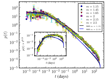
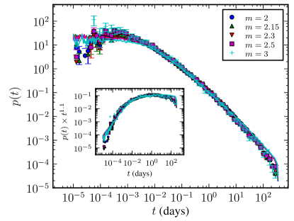
We turn now to the statistics of recurrence time intervals $t$, which are associated with the edges of the recurrence network. The comparison between the empirical catalogs and the ETAS model is shown in Fig 3. It can be seen that, with the parameters used for the ETAS model, and accounting properly for the missing data, the agreement between the datasets is excellent. Note that deviations for short time intervals are largely within the statistical uncertainties, but a lack of resolution and missing data in the empirical data not accounted for certainly play a role as well. This is further supported by the fact that there are basically no significant deviations for the Parkfield sequence which benefits from the higher quality of the seismic network in the region.

As the insets of Fig 3 indicate, after a characteristic time, which is independent of the magnitude threshold $m$, the probability density functions (PDF) $p(t)$ of the time intervals decay as $t^{-0.9}$ and $t^{-1.1}$ for Parkfield and Hector Mine, respectively. If one does not account for missing data in the ETAS models, the exponents of the power-law decay are unchanged but there are significant and systematic deviations at small time scales (not shown). In particular, the characteristic time varies with $m$. This is not only further evidence that it is crucial to take the effect of missing data into account but it also indicates that the characteristic time — which is of the order of a minute — might be an observational artifact.

Further support comes from the NHP model which predicts $p(t)$ as shown in the upper panel of Fig. 3 for Parkfield and different magnitude thresholds $m$ (see Appendix .2 for details). Indeed, the apparent lack of variation in $p(t)$ with respect to $m$ for the NHP model is due to the dependence of the parameters in the Omori law given in Eq. (9) on the magnitude threshold. In particular, the change in $c$ — which is typically related to missing data — prevents any significant variation in the characteristic time which would be expected otherwise (see Eq. (16)). However, the NHP model also shows a faster decay than what is actually observed for larger values of $t$. In fact, Eq. (16) predicts that we should not expect a pure power-law for Parkfield but rather a power-law with logarithmic corrections. We attribute this difference between the NHP model on one side and the ETAS model and the empirical data on the other side to the presence of spatiotemporal correlations. Clearly, this implies that at least some of the spatiotemporal correlations present in the empirical data are correctly captured by the ETAS model.

Figure 3: Probability density functions of the time intervals between an event and its recurrences for different threshold magnitudes $m$, for Parkfield (above) and Hector Mine (below). Solid lines represent results obtained for the ETAS model, and symbols for the empirical catalogs. The additional solid lines in the upper panel correspond to curves obtained with the NHP model. The insets show the rescaled functions as indicated by the axis labels.

4.3 Spatial recurrence statistics

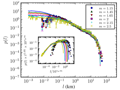
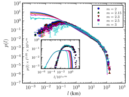
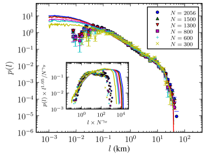
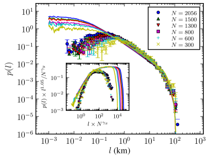
In addition to the time interval, there is also the spatial distance $l$ associated with each edge of the network. The PDF of these distances $p(l)$ for both the empirical and ETAS catalogs are shown in Figs. 4 and 5 for different magnitude thresholds $m$ and different numbers of events $N$, respectively. Contrary to the temporal statistics, there are significant differences between the ETAS model and the empirical data.

For the empirical data, $p(l)$ increases for small distances up to a characteristic distance followed by a decay for larger arguments . The decaying part itself consists of two regimes, a power-law decay for intermediate and large distances and a much faster decay for the largest arguments. The latter is simply a finite size effect since the maximal spatial extent of the aftershock sequences is about $40$km for Parkfield and about $150$km for Hector Mine. For both Parkfield and Hector mine, the power-law decay has the same exponent of about $1.05$ as evident from the insets of Figs. 4 and 5. The inset of Fig. 4 also shows that in both cases the characteristic distance scales as $10^{0.45m}$ with magnitude threshold $m$, while it scales as $N^{-0.45}$ with the number of considered events $N$ (inset of Fig. 5). Since $N\propto 10^{-m}$ according to the Gutenberg-Richter law for $b=1$, both scaling laws are trivially related in this case. As a comparison of the insets of Fig. 5 shows, the only obvious difference between the aftershock sequences of Parkfield and Hector mine are the constant prefactors in the respective scaling laws. This can be attributed to the different geometry of the faults in the areas considered. It is important to realize that all these findings are not significantly different from those for the NHP model (see Eq. (14, 15)) suggesting that they do not reflect any non-trivial spatiotemporal correlations.

For the ETAS model (see Figs. 4 and 5), $p(l)$ shows a similar behavior for large and intermediate distances but there are huge deviations at length scales smaller than the characteristic distance discussed above. While there is a characteristic distance for the ETAS model, it scales as $N^{-0.8}$ and $10^{0.8m}$, respectively  . This is not only different from the empirical data but there is also no obvious relationship to the spatial propagation of activity in the ETAS model defined by Eq. (4). Moreover, $p(l)$ does not increase for small distances but is clearly constant. Some of these differences can be reasonably attributed to the different dimensionality of the datasets: We have assumed for the ETAS model that the epicenters of the events are displaced in one dimension, in order to mimic the displacement along a single fault. However, this assumption breaks down exactly at small distances, since on those scales the higher-dimensional structure of the fault itself becomes important. To address this point, we have analyzed a version of the ETAS model for Parkfield where the events are distributed in a two-dimensional area. While this change in dimensionality does not affect the overall functional form of $p(l)$, the characteristic distance now scales as $N^{-0.45}$ and $10^{0.45m}$, respectively. Despite this agreement with the empirical data, the prefactor in the scaling of the characteristic distance is more than an order of magnitude larger. It is also important to note that $p(l)$ remains constant for small distances. This indicates that the spatial version of the ETAS model considered here is not able to reliably recover the spatial distribution of aftershocks on small scales. This is not unexpected since the isotropic spatial distribution of triggered events used in the ETAS model does not account for the orientations of the different faults and rupture areas. Surprisingly, however, the functional form of $p(l)$ and the scaling behavior of the characteristic distance observed for the empirical data can be well-reproduced by the NHP model (see Eq. (14, 15)) despite an isotropic spatial distribution of events in two dimensions. This is an indication that not necessarily the isotropy of the normalized spatial distribution of directly triggered events given in Eq. (4) is the issue but rather those spatiotemporal correlations that affect short spatial scales.

Figure 4: Recurrence distance distribution for different threshold magnitudes $m$, for Parkfield (above) and Hector Mine (below). Solid lines represent the respective ETAS model, and symbols correspond to the empirical catalogs. The insets show the rescaled distributions, with $\gamma_{x}=\gamma_{y}=0.45$ for both empirical data sets, $\gamma_{x}=0.8$ for both ETAS data sets, $\gamma_{y}=-0.1$ for the ETAS model of the Parkfield sequence and $\gamma_{y}=-0.15$ for the ETAS model of the Hector Mine sequence¹.

Figure 5: Recurrence distance distributions if only the first $N$ events after the mainshock are considered, for Parkfield with threshold magnitude $m=1.15$ (above) and Hector Mine with $m=2$ (below). Solid lines represent the respective ETAS model, and symbols correspond to the empirical catalogs. The insets show the rescaled distributions, with $\gamma_{x}=\gamma_{y}=0.45$ for both empirical data sets, $\gamma_{x}=0.8$ for both ETAS data sets, $\gamma_{y}=-0.1$ for the ETAS model of the Parkfield sequence and $\gamma_{y}=-0.15$ for the ETAS model of the Hector Mine sequence¹.

5 Discussion

It is interesting to compare the properties of the network of recurrences for the aftershock sequences associated with the Parkfield earthquake (September 28, 2004) and the Hector Mine earthquake (October 16, 1999) with those found for a 20-year catalog from southern California (Davidsen et al., 2008). For example, the out-degree distributions are clearly different: While they seem to follow a Poisson distribution for the isolated aftershock sequences, the distributions are significantly broader for the 20-year catalog. This indicates that spatiotemporal correlations exist between earthquakes that extend beyond what is typically considered an aftershock sequence. Another important finding is that the distributions of the time intervals between events and their recurrences are basically indistinguishable. Since the analysis of the ETAS model indicates that the absence of any dependence on the threshold magnitude for the aftershock sequences is a consequence of missing data, one can draw an analogous conclusion for the 20-year catalog. Finally, it is important to realize that the distributions of the spatial distance between an earthquake and its recurrences for the aftershock sequences do not show any indication of a non-trivial scaling with threshold magnitude. This is in sharp contrast to the 20-year catalog, which provided further evidence for a shadowing effect associated with smaller earthquakes (Rubin, 2002; Fischer and Horálek, 2005; Hainzl and Marsan, 2008). However, the absence of a shadowing effect might be attributed to the fact that the main events of both aftershock sequences studied here were of large magnitude — for which stress shadows are seldom observed (Helmstetter et al., 2005; Main, 2006) — and, hence, dominated the statistical behavior.

The comparison of the non-trivial statistical features of the network of recurrences for the aftershock sequences with those for the ETAS model showed that most of them are indeed correctly captured by the model if the effect of catalog incompleteness is taken into account. While this is a clear indication that some of the spatiotemporal correlations between earthquakes in aftershock sequences can be well-understood within the framework of the stochastic model, the significant differences in the spatial statistics of recurrences imply that the ETAS model is inadequate to explain all spatiotemporal correlations associated with aftershock sequences. Thus, our analysis confirms that the statistical properties of the network of recurrences can serve as a valuable benchmark test for models of seismicity as found in an earlier work on a conceptual model of earthquake dynamics (Peixoto and Davidsen, 2008). It remains to be seen whether other stochastic models of seismicity pass this test (Vere-Jones, 2005; Turcotte et al., 2007).

Appendix A

.1 Numerical simulation of the ETAS model

An artificial earthquake catalog can be created in an efficient manner with the ETAS model as follows. Starting from an initial event of magnitude $M$ at the origin, and at time $t=0$, the number of daughter events is sampled from a Poisson distribution with average $\rho(M)$. For each daughter event $i$, its magnitude, position, and occurrence time are independently sampled from $P(m_{i})$, $\Phi(\vec{r}_{i},m_{i})$ and $\Psi(t_{i}-t)$, respectively. The same procedure is then repeated for each daughter event, recursively, until there are no more events to be generated up to a predetermined maximum time. Background events, which are not daughters of any other event, can also be added, and their daughters can be obtained in the same manner. Thus, the total number of iterations is proportional to the number of events in the final catalog. The final rate of occurrence at a given time, considering all daughter events, is then given by

$$\lambda(t)=\lambda_{b}+\sum_{t_{i}<t}K10^{\alpha(m_{i}-m_{0})}\frac{\theta c^{\theta}}{(t-t_{i}+c)^{1+\theta}},$$ (8)

where $K=n(b-\alpha)/b$, $\lambda_{b}$ is the constant rate of background events, and the sum is taken over all previous events in the catalog.

.2 Simple non-homogeneous Poisson model

We follow the same approach as in Davidsen et al. (2008) which allows us to define a simple non-homogeneous Poisson (NHP) model by specifying the functions $\mu_{l}(l)$ and $\mu_{t}(t)$. These functions quantify the spatial and temporal distribution of events with respect to some reference event, respectively. Note that this fact trivially excludes the existence of any spatiotemporal correlations between events. In contrast to (Davidsen et al., 2008), we assume here that the rate of activity is not constant but given by the modified Omori law,

$$n\left(t\right)=\frac{K}{\left(t+c\right)^{p}},$$ (9)

where we restrict ourselves to the case $p>1$ as observed for Parkfield (Shcherbakov et al., 2006). We note that $p$ is not the same as $\theta+1$ in Eq. (3) for the ETAS model, since the latter describes the rate of events directly triggered by a single event, while the former describes the total event rate. Despite this non-homogeneous rate of activity, some of the statistical properties of the network of recurrences remain unchanged, including the topological structure, since they only depend on the spatial characteristics of the point process and the temporal ordering (Davidsen et al., 2008). Incorporating further the effect of finite space-time domains, we have

$$\mu_{l}(l)=2al\Theta\left(L-l\right),$$ (10)

$$\mu_{t}(t,t_{0})=\frac{K}{\left(c+t+t_{0}\right)^{p}}\Theta\left(T-t-t_{0}\right).$$ (11)

Here, $a$ is some constant such that $\mu_{l}(l)$ describes a homogeneous distribution of events in a two-dimensional ball of radius $L$ around the reference event. Hence, we assume translational invariance in space. $T$ corresponds to the finite observation period after the mainshock occurring at time $t=0$. $t_{0}$ is the time of occurrence of the reference event. Using the formalism presented in Davidsen et al. (2008), one can compute the average PDFs of finding a recurrence at distance $l$ from or at time $t$ after a randomly chosen reference event . This leads to

$$p_{l}(l)=\frac{2}{l}-\frac{2}{l^{3}}\frac{\left(p-1\right)}{aK}\frac{1}{\frac{1}{c^{p-1}}-\frac{1}{\left(c+T\right)^{p-1}}}\left[1-e^{-l^{2}aK\frac{1}{p-1}\left(\frac{1}{c^{p-1}}-\frac{1}{\left(c+T\right)^{p-1}}\right)}\right]\Theta\left(L-l\right),$$ (12)

$$p_{t}(t)=\frac{\left(p-1\right)}{\frac{1}{c^{p-1}}-\frac{1}{\left(c+T\right)^{p-1}}}\int_{0}^{\infty}\frac{p-1}{\left(c+t_{0}\right)\left(c+t+t_{0}\right)^{p}-\left(c+t_{0}\right)^{p}\left(c+t+t_{0}\right)}\times$$ (13)

$$\qquad\qquad\qquad\times\left[1-e^{-L^{2}aK\frac{1}{p-1}\left(\frac{1}{\left(c+t_{0}\right)^{p-1}}-\frac{1}{\left(c+t+t_{0}\right)^{p-1}}\right)}\right]\Theta\left(t-t-t_{0}\right)\,\mathrm{d}t_{0}.$$

The functional behavior of these PDFs can be broken down into several parts. For $p_{l}(l)$, we find

$$p_{l}(l)=\begin{cases}l\frac{aK}{\left(p-1\right)}\left(\frac{1}{c^{p-1}}-\frac{1}{\left(c+T\right)^{p-1}}\right)&l\ll l^{*}\\ \frac{2}{l}&l^{*}\ll l<L\\ 0&l>L,\end{cases}$$ (14)

where the characteristic distance $l^{*}$ scales as

$$l^{*}\propto\left[aK\frac{1}{2\left(p-1\right)}\left(\frac{1}{c^{p-1}}-\frac{1}{\left(c+T\right)^{p-1}}\right)\right]^{-\frac{1}{2}}\propto\frac{L}{\sqrt{N/2}}.$$ (15)

Note that the total number of events $N$ is simply given by $N=aL^{2}\int^{T}_{0}n(t)dt$. A comparison with the results derived in Ref. (Davidsen et al., 2008) for a homogeneous rate of activity shows that the qualitative features and the scaling exponents are unchanged. For $p_{t}(t)$, we have

$$p_{t}(t)\approx\begin{cases}\frac{p-1}{\frac{1}{c^{p-1}}-\frac{1}{\left(c+T\right)^{p-1}}}\frac{L^{2}aK}{2p-1}\left(\frac{1}{c^{2p-1}}-\frac{1}{\left(c+T\right)^{2p-1}}\right)&t\ll c\quad\wedge\quad t<\frac{c^{p}}{L^{2}aK}\\ \frac{1}{t}&t\ll c\quad\wedge\quad t>\frac{(c+T)^{p}}{L^{2}aK}\\ \text{see Eq.~{}(\ref{eq:large-values})}&t>c\quad\wedge\quad t<\frac{T+c}{2}\quad\wedge\quad t<T\\ 0&t>T.\end{cases}$$ (16)

$$p_{t}(t)\approx\frac{\left(p-1\right)^{2}}{\frac{1}{c^{p-1}}-\frac{1}{\left(c+T\right)^{p-1}}}\left\{\frac{1}{t^{p}}\ln\left(\frac{t}{c}\right)+\frac{1}{\left(p-1\right)^{2}}\left[\frac{1}{t^{p}}-\frac{1}{t\left(T-t+c\right)^{p-1}}+\right.\right.$$ (17)

$$\left.\left.\frac{p-1}{pt}\left(aL^{2}Kt\right)^{\frac{1-p}{p}}\left[\Gamma\left(\frac{p-1}{p},aL^{2}K\frac{1}{t^{p-1}}\right)-\Gamma\left(\frac{p-1}{p},aL^{2}K\frac{t}{\left(T-t+c\right)^{p}}\right)\right]\right]\right\},$$

where $\Gamma\left(\cdot,\cdot\right)$ denotes the incomplete Gamma function . Note that depending on the exact parameter values the $1/t$ regime might be present or not . For the aftershock sequence of Parkfield, one can also obtain $p_{t}(t)$ by numerically integrating Eq. (13). The values of the constants in Eqs. (10,11) can be derived from the values estimated for the Omori law given in  Shcherbakov et al. (2006). Note that the values of $c$ and $K$ vary with the magnitude threshold $m$. The variation in $c$ can arise due to missing data — see Shcherbakov et al. (2004, 2006), however, for a different interpretation. For $m=2.15$, we have $c=0.016$ d and $aL^{2}K=21$ d^p-1. For $m=1.15$, we have $c=0.08$ d and $aL^{2}K=200$ d^p-1. These curves are plotted in Fig. 3.

For $T\to\infty$ and $L\to\infty$, Eqs. (13,16) reduce to

$$p_{t}(t)=\left(p-1\right)c^{p-1}\int_{0}^{\infty}\frac{p-1}{\left(c+t_{0}\right)\left(c+t+t_{0}\right)^{p}-\left(c+t_{0}\right)^{p}\left(c+t+t_{0}\right)}\,\mathrm{d}t_{0}.$$ (18)

$$p_{t}(t)\approx\begin{cases}\frac{1}{t}&t\ll t^{*}\\ \frac{\left(p-1\right)^{2}c^{p-1}}{t^{p}}\left[\ln\left(\frac{t}{c}\right)+\frac{1}{\left(p-1\right)^{2}}\right]&t\gg t^{*},\end{cases}$$ (19)

where $t^{*}\propto c$.