Cavity-water interface is polar

Abstract

We present the results of numerical simulations of the electrostatics and dynamics of water hydration shells surrounding Kihara cavities given by a Lennard-Jones (LJ) layer at the surface of a hard-sphere cavity. The local dielectric response of the hydration layer substantially exceeds that of bulk water, with the magnitude of the dielectric constant peak in the shell increasing with the growing cavity size. The polar shell propagates into bulk water to approximately the cavity radius. The statistics of the electrostatic field produced by water inside the cavity follow linear response and approach the prediction of continuum electrostatics with increasing cavity size.

Nanoscale interfaces of polar liquids combine strong distortions of the liquid density profile with highly perturbed long-range electrostatic correlations. The interfacial density, and the related diffusional dynamics, are governed by short-range packing restrictions and are relatively short-ranged. Nevertheless, the density fluctuations of the interfacial region are critical for the long-range hydrophobic forces Ball:08 ; ChandlerNature:05 and the related weak dewetting of interfaces of non-polar solutes HummerPRL:98 ; Berne:09 . In contrast, electrostatic interactions, and the orientational correlations of multipolar moments, are long-ranged. They are assigned macroscopic length-scale in the Maxwell (continuum) electrostatics propagating the effect of partial charges at dielectric interfaces on the length-scale of the Coulomb potential. Whether this picture is correct for polar liquids and how the surface polarization is screened by the mobile liquid dipoles remains an open question DMepl:08 , the resolution of which will define the limits of continuum electrostatics in application to nanoscale interfaces of molecular liquids.

Water presents a particular challenge to the problems of interfacial dynamics and thermodynamics since energetically strong hydrogen bonds add a short-range scale competing with long-range electrostatic forces. The properties of hydration layers surrounding nanoscale solutes indeed turn out to be unusual. Apart from ubiquitous hydrophobic interactions linked to the structure of the water interface Ball:08 , measurements of microscopic electrostatics of the protein/water interface have shown some surprising results. Electrostatics on the microscopic scale is traditionally probed by the dynamic and static band-shifts of optical dyes Jimenez:94 . The corresponding Stokes-shift dynamics at the protein/water interface showed a long exponential decay absent for the free chromophores in solution. This observation has prompted the label of “biological water” for hydration layers of biopolymers Pal:04 . While the cause of this effect is still debated Zhang:07 ; Nilsson:05 , various extent of slowing of the collective Stokes shift dynamics has been universally observed at protein/water interfaces Pal:04 ; Zhang:07 . Further, the hydration shells around proteins were found to carry high local polarity DMpre2:08 , thus linking the slower dynamics to the structural reorganization of water in the form of a polarized cluster around proteins Ebbinghaus:07 . Unfortunately, the problem of the protein hydration is inseparable from the complex protein dynamics Frauenfelder:09 . Studies excluding this latter component are therefore necessary to understand the electrostatics of hydration layers when the solute size grows to the nanoscale. This is the goal of this report.

Here we present extensive Molecular Dynamics (MD) simulations of the structure of water around non-polar solutes (cavities). In contrast to previous active research in this field ChandlerNature:05 ; HummerPRL:98 ; Berne:09 ; GardePRL:09 , we ask here the following questions: (i) how polar is the interface? (ii) how far into the bulk does the polarity perturbation propagate? and (iii) how are the orientational dipolar dynamics of the hydration layers affected by the solute? The main result of this study is the observation of a significant increase of the local water polarity at the interface, with the region of enhanced polarity extending into the bulk to approximately the cavity radius.

The water nanoscale interface was modeled by inserting spherical solutes carrying a hard-sphere (HS) core surrounded by a Lennard-Jones (LJ) potential layer. The interactions with the SPC/E oxygen is then given by the Kihara solute-solvent potential

$$\phi(r)=4\epsilon_{\text{LJ}}\left[\left(\frac{\sigma}{r-r_{HS}}\right)^{12}-\left(\frac{\sigma}{r-r_{HS}}\right)^{6}\right].$$ (1)

The LJ well has the width $\sigma=3$ Å and the energy $\epsilon_{\text{LJ}}$ for which two values were used: $\epsilon_{\text{LJ}}=0.65\mbox{ kJ/mol}$ equal to the LJ energy between oxygens of SPC/E water and $\epsilon_{\text{LJ}}=20\mbox{ kJ/mol}$ close to the energy of hydrogen bonds in bulk water. The cavity size was varied by changing the HS radius $r_{\text{HS}}$ in the range 0–12 Å. The number of waters in the simulation cell was varied to allow sufficiently large solvation layers, with 4053 and 11845 hydration waters used for the smallest and largest solutes, respectively. The trajectories for analysis were 5 ns long, following 100–500 ps equilibration. Simulations were performed with cubic periodic boundary conditions, at 273 K and zero pressure, with Berendsen thermostat and barostat and a timestep of 2 fs. Ewald sums with tin foil boundary conditions were used for electrostatic interactions.

A spherical solute induces a spherical symmetry breaking in an otherwise isotropic liquid. The orientational structure of the interface consistent with this imposed symmetry is characterized by the first- and second-order orientational order parameters: $p_{1}(r)=(N(r))^{-1}\left\langle\sum_{r_{j}<r}\mathbf{\hat{r}}_{j}\cdot\mathbf{\hat{m}}_{j}\right\rangle$ and $p_{2}(r)=(2N(r))^{-1}\left\langle\sum_{r_{j}<r}[3(\mathbf{\hat{r}}_{j}\cdot\mathbf{\hat{m}}_{j})^{2}-1]\right\rangle$. These parameters project the unit dipolar vectors $\mathbf{\hat{m}}_{j}$ within the shell of radius $r$ on the radial direction $\mathbf{\hat{r}}_{j}=\mathbf{r}_{j}/r_{j}$, $N(r)$ is the number of waters within the shell. The first hydration layer is then defined as $R\leq r\leq R+1.5$ Å, $R=r_{\text{HS}}+\sigma$ and the corresponding order parameters are $p_{1}^{I}$ and $p_{2}^{I}$.

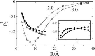
Figure 1: The second-order orientational order parameter $p_{2}^{I}$ of the water first shell vs the cavity radius $R=r_{\text{HS}}+\sigma$. The solid diamonds and triangles refer to cavities in water with $\epsilon_{\text{LJ}}=0.65$ and 20 kJ/mol, respectively. The open points refer to cavities in the fluid of dipolar hard spheres DMepl:08 with the reduced dipole moments $(m^{*})^{2}=\beta m^{2}/\sigma_{s}^{3}$ equal to 2.0 (open squares) and 3.0 (open circles); $m$ is the dipole moment and $\sigma_{s}$ is the hard-sphere diameter of the solvent. The inset shows the orientational parameter $p_{1}^{I}$ of the first hydration layer.

The dielectric constant of a cavity-water mixture can be defined in terms of the volume occupied by the cavity relative to the volume of water Scaife:98 . The solute-solvent response function describing the interfacial polarization can then be calculated by accounting for dipolar fluctuations accumulated within a radial water layer surrounding the cavity $\chi(r)=\beta\langle(\delta\mathbf{M}(r))^{2}\rangle/(3V(r))$; $\beta=1/(k_{\text{B}}T)$ is the inverse temperature. The water dipole moment $\mathbf{M}(r)$ in this equation is taken over the radial shell between the spherical cavity and radius $r$ extending from the cavity center to the bulk, $V(r)$ is the shell volume. The limit of infinite dilution yields the bulk dielectric susceptibility of water $\chi=\chi(\infty)=(\epsilon-1)/(4\pi)$, where $\epsilon$ is the water dielectric constant.

The fluctuation susceptibility $\chi(r)$ determines the dielectric constant $\epsilon(r)$ accumulated within the radial layer. For simulations employing periodic boundary conditions with tin-foil boundary around replicas of the simulation cell the connection between the simulated variance of the dipole moment and the dielectric constant is particularly simple Neumann:86 : $\epsilon(r)=1+4\pi\chi(r)$. The macroscopic dielectric constant of water is then $\epsilon=\epsilon(\infty)$.

The orientational structure of polar liquids at interfaces is strongly affected by short-range orientational correlations. Unsaturated hydrogen bonds of surface waters produce preferential in-plane orientations of water’s dipoles Lee:84 as reflected by the first and second orientational order parameters (Fig. 1). The first-order parameter $p_{1}^{I}$ is nearly zero pointing to no preferential radial orientation (inset in Fig. 1), while $p_{2}^{I}$ is non-zero and negative, in accord with the preferential in-plane orientation of the dipoles. This orientational pattern is specific for water and does not necessarily repeat itself in other polar liquid. For comparison, $p_{2}^{I}$ of hard-sphere dipoles at the surface of a spherical cavity DMepl:08 passes through a minimum (Fig. 1). Orientational order first grows with increasing cavity size as frustrations of dipolar orientations are released with the growing number of dipoles. However, further increase of the cavity size leads to a weak dewetting of the interface by the puling force of the liquid HummerPRL:98 with the resulting destruction of the interfacial orientational order. In contrast, water preserves its parallel interfacial order, mostly determined by its hydrogen-bond network and not much effected by the strength of the solute-solvent LJ attraction (Fig. 1).

The function $\epsilon(r)$ calculated for shells around cavities is compared to the same function calculated from shells around Lorentz’s virtual cavity Scaife:98 (water molecules between radii $R$ and $r$) taken from configurations of pure water without cavity inserted. The difference of the two functions shows a sharp peak (Fig. 2a) pointing to an effectively higher polarity of hydration shells around cavities compared to shells in bulk water.

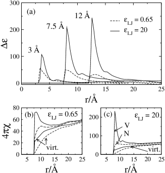
Figure 2: Dielectric constant of the hydration layer relative to the dielectric constant of the same layer around a virtual cavity for three cavity sizes indicated in the plot (a). The solid and dashed lines refer to $\epsilon_{\text{LJ}}=20$ and 0.65 kJ/mol, respectively. The response functions defined through the volume of the shell (“V”, solid lines) and through the number of shell waters (“N”, dashed lines) are shown in (b) for $\epsilon_{\text{LJ}}=0.65$ kJ/mol and in (c) for $\epsilon_{\text{LJ}}=20$ kJ/mol; $R=7.5$ Å. $\chi(r)$ for the virtual cavity is marked as “virt.”

In order to distinguish between the orientational and density origins of the peak in the dielectric constant, we have plotted in Figs. 2(b,c) $\chi(r)$ defined as above in comparison with the susceptibility normalized to the number of waters in the shell $N(r)$: $\chi_{N}(r)=\beta\rho\langle(\delta\mathbf{M}(r))^{2}\rangle/(3N(r))$, where $\rho$ is the number density of bulk water. This comparison shows that the origin of $\Delta\epsilon$ is a composite effect of changes in both the local density and orientational structure. Even though a significant part of $\Delta\epsilon$ comes from the increased density in the first solvation layer, particularly at the large solute-solvent LJ attraction (Fig. 2(c)), the effect cannot be cast in terms of $N(r)$ only.

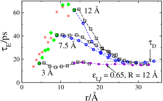
Figure 3: Exponential relaxation time of $\chi^{I}(t)$ (closed diamonds), $C_{E}(r,t)$ (open circles), and $\chi(r,t)$ (open squares); $\epsilon_{\text{LJ}}=20$ kJ/mol. Also shown is the exponential relaxation time of the self-correlation function of the unit vector $\mathbf{\hat{e}}^{I}(t)$ representing the dipole moment of the first-shell waters. Different cavity sizes for the $r$-dependent relaxation times are indicated in the plot. The filled circles refer to $R=12$ Å and $\epsilon_{\text{LJ}}=0.65$ kJ/mol and the horizontal dotted line indicates the Debye relaxation time $\tau_{D}$ of pure SPC/E water. The dashed lines in the plot are connecting the points.

Given the long range of the interfacial orientational order one wonders how the dynamics of hydration layers are affected. We have looked at several correlation functions. $\chi^{I}(t)=\beta\langle(\delta\mathbf{M}^{I}(t)\cdot\delta\mathbf{M}^{I}(0)\rangle/(3V^{I})$ is the time self-correlation function of the dipole moment of the first solvation layer and $\chi(r,t)$ is a similar correlation function extended to a layer within the radius $r$ from the cavity’s center. In addition, we have calculated the correlation function $C_{E}(t)=\langle\delta\mathbf{E}_{s}(r,t)\cdot\delta\mathbf{E}_{s}(r,0)\rangle$ of the electric field $\mathbf{E}_{s}(r,t)$ produced at the cavity’s center by the waters within the $r$-shell. This latter correlation function represents the Stokes shift dynamics of dipolar chromophores Pal:04 ; Zhang:07 . All correlation functions were fitted to a sum of a ballistic Gaussian decay and an exponential tail Jimenez:94 . Figure 3 presents the compilation of the results for the exponential relaxation time $\tau_{E}$.

The main observation from the dynamics calculations is a significant growth of the exponential relaxation time of the first solvation layer with the cavity size (filled diamonds in Fig. 3). Consistent with the results for $\Delta\epsilon(r)$, this dynamics perturbation propagates into the bulk to at least the distance of the cavity radius. The exponential decay time of $C_{E}(r,t)$ retraces the corresponding time from $\chi(r,t)$. The dipolar dynamics of the first solvation layer are dominated by rotations of the dipole moment $\mathbf{M}^{I}$, instead of its magnitude fluctuations, as is seen from the self-correlation function of the unit vector $\mathbf{\hat{e}}^{I}(t)=\mathbf{M}^{I}(t)/M^{I}(t)$ (crosses in Fig. 3). This observation points to a high level of orientational cooperativity in the first solvation layer, which does not decorrelate by individual dipole rotations and instead rotates slowly as a correlated dipolar domain. This dynamical slowing is however seen only for the larger LJ attraction, $\epsilon_{\text{LJ}}=20$ kJ/mol, and no effect of the solute on the dynamics is observed when the solute-solvent LJ potential is similar to that in water, $\epsilon_{\text{LJ}}=0.65$ kJ/mol (closed points in Fig. 3). This result might help to explain the conflicting literature He:07 on the subject of the surface-induced alteration of the liquid dynamics. The outcome seems to be controlled by the strength of the solute-solvent interactions and thus the surface composition.

Our results partially support Onsager’s concept of “inverted snowball” dynamics Onsager:77 . It stipulates that solvation dynamics are slower close to a newly created charge compared to more distant layers, ranging between the one-particle (slow) orientational diffusion and the dielectric (fast) relaxation of the bulk. The data in Fig. 3 indeed show a speedup of dipolar relaxation into the bulk. However, this effect strongly depends on both the cavity size and the solute-solvent LJ interaction. It is expected to be essentially absent for typical optical probes Jimenez:94 consistent in size with the smallest cavity studied here. Further, even for larger cavities, the slow dynamics of the closest solvation layers are almost lost when the hydration layer is grown to the boundaries of the simulation cell. At that point, the relaxation time becomes the Debye relaxation time of bulk water (Fig. 3). This observation implies that dipolar optical probes placed inside the cavity Pal:04 ; Zhang:07 ; Nilsson:05 will not pick up the slowing of the closest hydration shells and instead will average the effect out by the electric field contributions from more distant layers.

The statistics of dipolar interfacial fluctuation can be probed by the chemical potential of electrostatic solvation, i.e. the free energy of interaction of the charges inside the cavity with the surrounding water solvent. We found that the dipolar field $\mathbf{M}(r)$ is Gaussian and thus the linear response approximation should be applicable. The solvation chemical potential of a charge $\mu_{q}$ or a dipole $\mu_{d}$ can then be found from the variance of the electrostatic potential $\phi_{s}$ or the electric field $\mathbf{E}_{s}$ produced by the solvent at the position of the corresponding multipole Ben-Amotz:05 : $\mu_{q}=-\beta(q_{0})^{2}\langle(\delta\phi_{s})^{2}\rangle/2$, $\mu_{d}=-\beta(m_{0})^{2}\langle(\delta\mathbf{E}_{s})^{2}\rangle/6$. Here, $q_{0}$ and $m_{0}$ are, correspondingly, the charge and point dipole within the cavity. The averages in these relations do not depend, in linear response, on whether the corresponding multipoles are actually present inside the cavity Ben-Amotz:05 . They can therefore be calculated from our simulations with empty cavities providing insights into how these solvation free energies scale with the size of the solute and whether the limit of continuum electrostatics is reached.

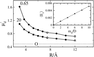
Figure 4: Chemical potential $\mu_{d}^{*}=\mu_{d}m_{0}^{2}/R^{3}$ of solvating the point dipole $m_{0}$ at the center of the cavity of radius $R$. The solid points ($\epsilon_{\text{LJ}}=20$ kJ/mol, circles and 0.65 kJ/mol, squares) and obtained from the variance of the water electric field inside the empty cavity, $\mu_{d}\propto\langle(\delta E_{s})^{2}\rangle$. The open triangles are from the thermodynamic integration of the average electric field $\langle E_{s}\rangle$ produced by dipoles of increasing magnitude ($0<m_{0}<10$ D) positioned at the cavity center. The average field (eV/D) is a linear function of the dipole magnitude $m_{0}$ (inset, $R=12$ Å, $\epsilon_{\text{LJ}}=0.65$ kJ/mol). The dashed line in the inset is the prediction based on the field variance inside the empty cavity (not the best fit). The dotted horizontal line is the result of continuum electrostatics given by the Onsager relation (“O”).

We found noticeable effects of the size of the simulation cell on $\langle(\delta\phi_{s})^{2}\rangle$ and much smaller size effects on $\langle(\delta\mathbf{E}_{s})^{2}\rangle$. We have therefore chosen to look at the statistics of the field fluctuations and the corresponding chemical potential of dipole solvation. These results are summarized in Fig. 4 showing $\mu_{d}^{*}=\mu_{d}R^{3}/(m_{0})^{2}$. This dimensionless parameter is expected to approach, with growing cavity size, the size-independent limit of continuum electrostatics, given by the Onsager equation Scaife:98 $\mu_{d}=(\epsilon-1)/(2\epsilon+1)\simeq 0.5$. The values of $\mu_{d}$, although noticeably higher at intermediate sizes, indeed seem to approach this limit. The open points in Fig. 4 are obtained by thermodynamic integration of average energies of point dipoles placed at the cavity center. A good agreement between $\mu_{d}$ from the field variance and from the thermodynamic integration, as well as the linear dependence of $\langle E_{s}\rangle$ vs $m_{0}$ (inset in Fig. 4), testifies to the validity of the linear response approximation.

The chemical potential $\mu_{d}$ is not strongly affected by the strength of the solute-solvent LJ attraction. The range of $\epsilon_{\text{LJ}}$ values studied here probably covers most of situations of practical interest. Deviations of the electric field variance from the area between the two curves shown in Fig. 4 might therefore be used to identify nonlinear solvation typically associated with hydrogen bonding between water and the solute DMjpca1:06 .

The results obtained here must have significant implications for self-assembly of nano-sized objects and biological activity of hydrated biopolymers. Polar solvation layers around solutes are expected to screen the inside charges. In the crowded environment of a living cell Douglas:09 this screening will reduce interactions between multipolar solutes. The high-polarity layer is also characterized by slower dipolar solvation. However, this effect is is not picked up by the dynamics of dipolar probes placed inside the cavity. A slow relaxation component observed in optical time-resolved spectra Pal:04 therefore needs to be assigned to protein motions pushing the hydration layers Nilsson:05 .

- (1) P. Ball, Chem. Rev. 108, 74 (2008)
- (2) D. Chandler, Nature 437, 640 (2005)
- (3) G. Hummer and S. Garde, Phys. Rev. Lett. 80, 4193 (1998)
- (4) B. J. Berne, J. D. Weeks, and R. Zhou, Annu. Rev. Phys. Chem. 60, 85 (2009)
- (5) D. R. Martin and D. V. Matyushov, Europhys. Lett. 82, 16003 (2008)
- (6) R. Jimenez, et al. Nature 369, 471 (1994)
- (7) S. K. Pal and A. H. Zewail, Chem. Rev. 104, 2099 (2004)
- (8) L. Zhang, et al. Proc. Natl. Acad. Sci. 104, 18461 (2007)
- (9) L. Nilsson and B. Halle, Proc. Natl. Acad. Sci. 102, 13867 (2005)
- (10) D. N. LeBard and D. V. Matyushov, Phys. Rev. E 78, 061901 (2008)
- (11) S. Ebbinghaus, et al. Proc. Natl. Acad. Sci. 104, 20749 (2007)
- (12) H. Frauenfelder, et al. Proc. Natl. Acad. Sci. 106, 5129 (2009)
- (13) S. Sarupria and S. Garde, Phys. Rev. Lett. 103, 037803 (2009)
- (14) B. K. P. Scaife, Principles of dielectrics (Clarendon Press, Oxford, 1998)
- (15) M. Neumann, Mol. Phys. 57, 97 (1986)
- (16) C. Y. Lee, J. A. McCammon, and P. J. Rossky, J. Chem. Phys. 80, 4448 (1984)
- (17) F. He, L.-M. Wang, and R. Richert, Eur. Phys. J. 141, 3 (2007)
- (18) L. Onsager, Can. J. Chem. 55, 1819 (1977)
- (19) D. Ben-Amotz, F. O. Raineri, and G. Stell, J. Phys. Chem. B 109, 6866 (2005)
- (20) P. K. Ghorai and D. V. Matyushov, J. Phys. Chem. A 110, 8857 (2006)
- (21) J. F. Douglas, J. Dudowicz, and K. F. Freed, Phys. Rev. Lett. 103, 135701 (2009)