Dynamic Bertrand Oligopoly

Abstract

We study continuous time Bertrand oligopolies in which a small number of firms producing similar goods compete with one another by setting prices. We first analyze a static version of this game in order to better understand the strategies played in the dynamic setting. Within the static game, we characterize the Nash equilibrium when there are $N$ players with heterogeneous costs. In the dynamic game with uncertain market demand, firms of different sizes have different lifetime capacities which deplete over time according to the market demand for their good. We setup the nonzero-sum stochastic differential game and its associated system of HJB partial differential equations in the case of linear demand functions. We characterize certain qualitative features of the game using an asymptotic approximation in the limit of small competition. The equilibrium of the game is further studied using numerical solutions. We find that consumers benefit the most when a market is structured with many firms of the same relative size producing highly substitutable goods. However, a large degree of substitutability does not always lead to large drops in price, for example when two firms have a large difference in their size.

1 Introduction

We study competitive markets with a small number of players in which firms use price as their strategic variable in an uncertain demand environment. These are known as Bertrand oligopolies. The firms are selling differentiated but substitutable goods. Many products, for instance consumer goods, are sold in markets that fit this structure. An example might be Pepsi and Coca-Cola in the market for soft drinks. Oil, coal and natural gas are commodities that can be substituted for one another for energy production, but which have different prices per unit of energy produced.

In this paper, we analyze price setting competition in the case of differentiated goods, and in continuous time under randomly fluctuating demands. These are nonzero-sum stochastic differential games that may be characterized by systems of Hamilton-Jacobi-Bellman PDEs. The large literature on oligopolistic competition deals primarily with the static problem, and we refer to Friedman [18] and Vives [27] for background and references. Cournot [11] provided the first analysis of an oligopoly where firms’ strategic interactions are taken into account. He assumed that firms compete using quantity as their strategic variable and then take prices as determined by the market through an inverse demand function, that is, a mapping from quantity to price. In a scathing review of Cournot’s paper, Bertrand [7] argued that firms compete using price as their strategic variable and then produce to clear the market demand arising from a demand function, that is, a mapping from price to quantity. In actuality, some markets may be better modeled as Cournot, and others as Bertrand, and we do not enter that debate here.

In both these original models, however, the goods were homogeneous, that is perfectly substitutable. This means that the only difference between the firms is the price they set or the quantity they produce. In the price setting game, this induces the behavior that, if the prices between two goods are not equal, consumers will only purchase the lower priced good. Here, we do not assume goods are perfectly substitutable, and therefore, if firms have prices that differ, they may all still receive some demand from the market. Models of product differentiation originated with Hotelling [23] and Chamberlin [10], and were extended by d’Aspremont et al. [12], among others. See Friedman [18, Chapter 3] for an excellent discussion.

Most of the continuous-time models are in a linear-quadratic (LQ) set-up, which has convenient analytical properties. We refer to Engwerda [15] for details, and Hamadène [20] for an approach via BSDEs. Jun and Vives [24] work within the context of a differential game of a duopoly with differentiated products. Their general model allows for either Cournot or Bertrand competition in which the players control the rate of change of the rate of production or price, respectively, in the LQ setting.

There has been much recent interest in other types of stochastic differential games. We mention, for example, Lasry and Lions [25], who consider Mean Field Games in which there are a large number of players and competition is felt only through an average of one’s competitors, with each player’s impact on the average being negligible. Bensoussan et al. [6] study leader-follower differential games in real options problems. Ekeland and Pirvu [14] and Björk and Murgoci [9] analyze time-inconsistent control problems which can be viewed as games against one’s future self. Energy markets in which a small number of firms control supply can be viewed as Cournot oligopolies and they are analyzed in the context of exhaustible resources in Harris et al. [22].

The state variable of the firms in our model is their remaining lifetime capacity. This is a quantity whose value at time zero represents all of the possible production a firm can undertake over its lifetime before it goes out of business. The primary reason for this choice is that it is a natural way to capture the notion of relative sizes of firms. A firm with a very large lifetime capacity is a major market participant whose decisions greatly affect the prevailing price in the market. A firm with a very small lifetime capacity has very little market power. Here, we analyze the effect that participant size has on Bertrand markets over time. For producers of consumer goods, the lifetime capacities could be proxied by past volume of sales projected forward into the expected lifetime of the firm. In the case of exhaustible resources, the state variables would be estimates of remaining oil, coal or natural gas reserves, for instance.

In Section 2, we set up the static version of our price setting game and prove the existence and uniqueness of a Nash equilibrium. The resulting equilibrium price functions are inputs for Section 3 where we present the dynamic Bertrand game. We characterize the price strategies of the firms using the solution to a system of coupled nonlinear PDEs. We analyze in detail the problem of a duopoly with linear demand functions and the related monopoly problem. Analytically, we obtain an asymptotic expansion in powers of a parameter that represents the extent of competition between the firms in a deterministic game. In Section 4, we present the numerical solution of our system of PDEs that allows us to characterize the price strategies and resulting demands of firms in the stochastic game. Finally, in Section 5, we conclude and discuss further lines of research.

2 Static Bertrand Game

The main purpose of this paper is to analyze a dynamic price setting game in continuous time. In order to fully understand this game, we first analyze a static version of the game and prove existence and uniqueness of a Nash equilibrium. This is used in establishing the system of HJB PDEs of the dynamic game in the next section.

We assume a market with $N$ firms where each firm uses price as a strategic variable in noncooperative competition with the remaining firms. Associated to each firm $i\in\left\{1,\ldots,N\right\}$ is a variable $p_{i}\in\mathbb{R}_{+}$ that represents the price at which firm $i$ offers its good for sale to the market. We denote by $p$ the vector of prices whose $i$th element is $p_{i}$.

2.1 Systems of Demand

Given prices of the firms, we specify the resulting market demands for each firm’s good. For each firm $i\in\left\{1,\ldots,N\right\}$, there exists a demand function $D_{i}^{N}\left(p_{1},p_{2},\ldots,p_{N}\right):\mathbb{R}^{N}_{+}\rightarrow\mathbb{R}$. We first state some natural properties of these demand functions.

Assumption 2.1 (Properties of Demand Functions).

For all $i=1,\ldots,N$, $D^{N}_{i}$ is smooth in all variables, and

$$D^{N}_{N}(0,\ldots,0)>0,\qquad\frac{\partial D^{N}_{i}}{\partial p_{i}}<0,\qquad\mbox{and}\qquad\frac{\partial D^{N}_{i}}{\partial p_{j}}>0\textrm{ for }i\neq j.$$

We further assume that firms are distinguished only by the prices they set.

Assumption 2.2 (Exchangeability of Firms).

For fixed $p_{1},\ldots,p_{N}$ and all $i,j\in\left\{1,\ldots,N\right\}$,

$$D^{N}_{i}\left(p_{1},\ldots,p_{i},\ldots,p_{j},\ldots,p_{N}\right)=D_{j}^{N}\left(p_{1},\ldots,p_{j},\ldots,p_{i},\ldots,p_{N}\right).$$

This implies that the demand function is invariant under permutations of the other firms’ prices. That is, for any $j,k\in\left\{1,\ldots,N\right\}\backslash\left\{i\right\}$, we have

$$D^{N}_{i}\left(p_{1},\ldots,p_{i},\ldots,p_{j},\ldots,p_{k}\ldots,p_{N}\right)=D^{N}_{i}\left(p_{1},\ldots,p_{i},\ldots,p_{k},\ldots,p_{j}\ldots,p_{N}\right).$$

Smoothness of these functions is for convenience, and, naturally, the market has positive demand if the prices are low enough. The key assumption in the above is that demand for an individual firm is decreasing in the firm’s own price and increasing in the price of their rivals. This assumption implies that we only deal with substitute goods. A classical example is Coca-Cola versus Pepsi. However, such goods can also be of different kinds and thus not directly replaceable, yet they still exhibit substitutability. For example, an iPod and a compact disc. One cannot directly replace the other, but we expect a drop in the price of iPods to cause a drop in the demand for compact discs. Contrary to this type of good, there are goods known as complementary goods, such as hot dogs and hot dog buns, but we do not consider those kinds of competition here.

We now make additional convenient assumptions.

Assumption 2.3 (Finite Choke Price).

Fix a firm $i\in\left\{1,\ldots,N\right\}$. For any fixed set of prices $p_{-i}\triangleq\left(p_{1},\ldots,p_{i-1},p_{i+1},\ldots,p_{N}\right)$, we assume there exists a “choke price”, $\hat{p}_{i}\left(p_{-i}\right)<\infty$, such that

$$D^{N}_{i}\left(p_{1},\ldots,p_{i-1},\hat{p}_{i},p_{i+1},\ldots,p_{N}\right)=0.$$ (1)

Note that this “choke price” is unique by Assumption 2.1 because $\partial D^{N}_{i}/\partial p_{i}<0$. This price is also positive by the same assumption and Assumption 2.2 because $D^{N}_{N}\left(0,\ldots,0\right)=D^{N}_{i}\left(0,\ldots,0\right)>D^{N}_{i}\left(0,\ldots,0,\hat{p}\left(0\right),0,\ldots,0\right)=0$. This implies $\hat{p}_{i}\left(0\right)>0$.

Remark 2.1.

For example, suppose each firm’s demand depends on its rivals’ prices only through their sum: $D^{N}_{i}=f\left(p_{i},\sum_{j\neq i}p_{j}\right)$ where $f(x,y):\mathbb{R}_{+}\times\mathbb{R}_{+}\rightarrow\mathbb{R}$ is a smooth function which is increasing in $y$, decreasing in $x$, and such that there exists a solution $x$ to $f(x,y)=0$ for every $y$. Then, it is easy to see that this demand system satisfies Assumptions 2.1, 2.2 and 2.3.

The actual demand that each firm faces cannot be negative as the firms are suppliers. For a fixed price vector $p$, we define $D_{i}(p)$, without the superscript, as the actual demand firm $i$ receives in the market. Suppose first, for simplicity, that $p_{1}\leq p_{2}\leq\cdots\leq p_{N}$. If this is not the case, then we can re-order the firms, carry out the following procedure, and then return them to their original order once their demands have been determined. We next show that if prices are ordered, then this same ordering carries over to the demands.

Proposition 2.1 (Price order implies demand order).

Fix a vector of prices $p$. Suppose they are ordered such that $p_{1}\leq p_{2}\leq\cdots\leq p_{N}$. Then,

$$D^{N}_{1}\left(p_{1},\ldots,p_{N}\right)\geq D^{N}_{2}\left(p_{1},\ldots,p_{N}\right)\geq\cdots\geq D^{N}_{N}\left(p_{1},\ldots,p_{N}\right).$$

Proof.

Using the ordering of the prices, the properties of the derivatives of the demand functions, and Assumption 2.2, we have

$$D^{N}_{N}\left(p_{1},\ldots,p_{N-2},p_{N-1},p_{N}\right) = D^{N}_{N-1}\left(p_{1},\ldots,p_{N-2},p_{N},p_{N-1}\right)$$

$$\leq D^{N}_{N-1}\left(p_{1},\ldots,p_{N-2},p_{N-1},p_{N-1}\right)$$

$$\leq D^{N}_{N-1}\left(p_{1},\ldots,p_{N-2},p_{N-1},p_{N}\right).$$

The result then follows for all $D^{N}_{i}$ by applying the same procedure. ∎

To determine the actual demand $D_{i}(p)$, we begin with the demand function $D^{N}_{N}(p_{1},p_{2},\ldots,p_{N})$. If $D^{N}_{N}(p)\geq 0$, then it must be the case that $D^{N}_{i}(p)\geq 0$ for all $i=1,\ldots,N$ by Proposition 2.1. The actual demand that each firm faces is $D^{N}_{i}(p)$. Hence,

$$D_{i}(p)=D^{N}_{i}(p)~{}~{}\textrm{ for all }i=1,\ldots,N,$$

and all the demands are determined. Otherwise, if $D^{N}_{N}(p)<0$, then the price $p_{N}$ is too high relative to the preference structure of the market to make any sales in the market. Thus, this firm will receive no demand from the market and the demand of the remaining firms must reflect this fact. The demand for firm $N$ is set to zero, $D_{N}(p)=0$, and the demand for the remaining firms is determined by considering their residual demand functions, which we now define.

Let us consider the general case of residual demand for $n$ firms when all firms $i>n$ receive zero demand at the current set of prices.

Definition 2.1 (Consistency of Demand).

For each $n\in[1,N-1]$, we define the $n$-firm system of demand functions from the $(n+1)$-firm system of demand functions through

$$D_{i}^{n}\left(p_{1},p_{2},\ldots,p_{n}\right)=D_{i}^{n+1}\left(p_{1},p_{2},\ldots,p_{n},\hat{p}_{n+1}\right)\hskip 14.22636pt\textrm{ for }i=1,\ldots,n,$$

where $\hat{p}_{n+1}\left(p_{1},\ldots,p_{n}\right)$ is defined by $D^{n+1}_{n+1}\left(p_{1},\ldots,p_{n},\hat{p}_{n+1}\right)=0$.

Definition 2.1 encapsulates that, if firm $n+1$ sets price so high that $D^{n+1}_{n+1}(p)<0$, demands for firms $i<n+1$ are consistently adjusted as if firm $n+1$ set price $\hat{p}_{n+1}$ that realizes it exactly zero demand. This will give rise to actual demands which are continuous as a firm raises its price through the level at which it receives zero demand, and the market effectively has one less player. We shall see in Remark 2.3 that a common way of generating demand systems through a representative consumer’s utility maximization problem yields a demand system with this consistency property.

In Definition 2.1, we do not necessarily know that $\hat{p}_{n+1}$ exists for all $n$. We shall prove that they do exist in Proposition 2.2, but first we need to make one additional assumption.

Assumption 2.4.

For all $n\in[1,N-1]$ and all $i=1,\ldots,n$, we assume $\frac{\partial D^{n}_{i}}{\partial p_{i}}<0$.

We will see in Propositions 2.2 and 2.3 that the other natural properties of Assumptions 2.1, 2.2 and 2.3 are inherited by the lower level demand functions. However, it is necessary to assume that lower level demand functions are decreasing in each player’s own price.

Proposition 2.2.

For each $n\in[1,N-1]$, there exists a finite “choke price” $\hat{p}_{n+1}(p_{1},\ldots,p_{n})$ where

$$D^{n+1}_{n+1}\left(p_{1},\ldots,p_{n},\hat{p}_{n+1}\right)=0.$$

Proof.

See Appendix A. ∎

Proposition 2.3 (Inherited Demand Properties).

The functions $D_{i}^{n}$, as defined in Definition 2.1, are smooth in all variables, and $\frac{\partial D^{n}_{i}}{\partial p_{j}}>0\textrm{ for }i\neq j$, and $i=1,\ldots,n$.

The functions $D_{i}^{n}$ also inherit the symmetry of the functions $D_{i}^{N}$ from Assumption 2.2. Furthermore, they inherit the ordering of demand shown in Proposition 2.1. That is, for a fixed vector of prices $p$, ordered such that $p_{1}\leq p_{2}\leq\cdots\leq p_{N}$, we have for any $1\leq n\leq N$

$$D^{n}_{1}\left(p_{1},\ldots,p_{n}\right)\geq D^{n}_{2}\left(p_{1},\ldots,p_{n}\right)\geq\cdots\geq D^{n}_{n}\left(p_{1},\ldots,p_{n}\right).$$

Proof.

The smoothness of the functions $D_{i}^{n}$ clearly comes directly from that of $D^{N}_{i}$. Furthermore, the symmetry of these functions is also clearly inherited. To show the positive transverse derivative, we simply compute. We show only at the level $N-1$; for all $n\in[1,N-1]$, the property will follow in the exact same way from the function at the level $n+1$ using Assumption 2.4. We first take the derivative of Eqn. (1) with respect to $p_{j}$ for $j\neq N$, which gives

$$\frac{\partial\hat{p}_{N}}{\partial p_{j}}=-\frac{\partial D^{N}_{N}/\partial p_{j}}{\partial D^{N}_{N}/\partial p_{N}}>0,\mbox{ because }\frac{\partial D^{N}_{N}}{\partial p_{j}}>0\mbox{ and }\frac{\partial D^{N}_{N}}{\partial p_{N}}<0.$$

Then, for $i=1,\ldots,N-1$ and $j\in\left\{1,\ldots,N-1\right\}\backslash\left\{i\right\}$, we have

$$\frac{\partial D^{N-1}_{i}}{\partial p_{j}}=\frac{\partial D^{N}_{i}}{\partial p_{j}}+\frac{\partial D^{N}_{i}}{\partial p_{N}}\frac{\partial\hat{p}_{N}}{\partial p_{j}}.$$

This is positive because of Assumption 2.1 and because $\frac{\partial\hat{p}_{N}}{\partial p_{j}}>0$ for any $j\neq N$. With these properties, the ordering of demands follows by applying the exact same proof as Proposition 2.1. ∎

We can now specify completely the demand function that each firm faces for a given set of prices.

Definition 2.2.

(Actual Demands) Given an ordered price vector $p$:

• If $D_{N}^{N}(p)\geq 0$, then $D_{i}(p)=D^{N}_{i}(p)$ for all $i=1,\ldots,N$.

• Otherwise, find $n\in\left\{1,\ldots,N-1\right\}$ such that

  $$D^{n+1}_{n+1}\left(p_{1},\ldots,p_{n},p_{n+1}\right)<0,\qquad\textrm{ and }\qquad D^{n}_{n}\left(p_{1},\ldots,p_{n}\right)\geq 0.$$

  For such an $n$, the actual demands of firms $n+1,\ldots,N$ are equal to zero, and $D_{i}^{n}$ give the actual demands for each firm $i\in\left\{1,\ldots,n\right\}$:

  $$D_{i}(p)=\left\{\begin{array}[]{ccl}D^{n}_{i}\left(p_{1},p_{2},\ldots,p_{n}\right)&&\textrm{ for }i=1,\ldots,n\\ 0&&\textrm{ for }i=n+1,\ldots,N\end{array}\right.$$

• If no such $n$ exists, then $D_{i}(p)=0$ for all $i=1,\ldots,N$.

2.2 Example: Linear Demand

We present demand functions that are affine in the prices of all firms. This is the demand structure we will use in the dynamic game of the following sections. For fixed $N$, we start with positive parameters $A,B,C$ such that $B>(N-1)C$. This latter condition on the parameters will be justified in what follows. With these parameters, we define

$$D_{i}^{N}\left(p_{1},\ldots,p_{N}\right)\triangleq A-Bp_{i}+C\sum_{j\neq i}p_{j},~{}~{}\textrm{ for }i=1,\ldots,N.$$ (2)

Notice that $D^{N}_{N}(0,\ldots,0)=A>0$, and $D_{i}^{N}$ is of the form given in Remark 2.1. Therefore the demand functions satisfy Assumptions 2.1, 2.2 and 2.3.

Proposition 2.4.

For each $n\in[1,N-1]$, we have

$$D_{i}^{n}\left(p_{1},\ldots,p_{n}\right)=a_{n}-b_{n}p_{i}+c_{n}\sum_{\underset{j\leq n}{j\neq i}}p_{j},~{}~{}\textrm{ for }i=1,\ldots,n,$$ (3)

where, for $2\leq n\leq N$,

$$a_{n-1}=a_{n}\left(1+\frac{c_{n}}{b_{n}}\right),\qquad b_{n-1}=b_{n}\left(1-\frac{c_{n}^{2}}{b_{n}^{2}}\right),\qquad c_{n-1}=c_{n}\left(1+\frac{c_{n}}{b_{n}}\right),$$ (4)

with $a_{N}=A$, $b_{N}=B$ and $c_{N}=C$.

Proof.

Using Definition 2.1, we solve for the choke price $\hat{p}_{N}$ by setting $D_{N}^{N}$ in Eqn. (2) to zero and solving for $p_{N}$. This results in $\hat{p}_{N}=B^{-1}\left(A+C\sum_{i=1}^{N-1}p_{i}\right)$. Substituting into Eqn. (2) we obtain, for $i=1,\ldots,N-1$,

$$D_{i}^{N-1}(p_{1},\ldots,p_{N-1})=A\left(1+\frac{C}{B}\right)-B\left(1-\frac{C^{2}}{B^{2}}\right)p_{i}+C\left(1+\frac{C}{B}\right)\sum_{\underset{j\leq N-1}{j\neq i}}p_{j},$$

which establishes Eqn. (4) for $n=N$. We can repeat this procedure for $1\leq n\leq N-1$, where we find $\hat{p}_{n+1}=b_{n+1}^{-1}\left(a_{n+1}+c_{n+1}\sum_{i=1}^{n}p_{i}\right)$, and this results in the demand system at the level $n$ being given by Eqn. (3) with the recursively defined parameters given in Eqn. (4). ∎

Proposition 2.5.

The explicit solution of the recursion (4) is given by

$$a_{n}=\frac{\alpha}{\beta+(n-1)\gamma},\qquad b_{n}=\frac{\beta+(n-2)\gamma}{(\beta+(n-1)\gamma)(\beta-\gamma)},\qquad c_{n}=\frac{\gamma}{(\beta+(n-1)\gamma)(\beta-\gamma)},$$ (5)

where we define

$$\gamma=\frac{C}{\left(B-(N-1)C\right)\left(B+C\right)},\qquad\alpha=\gamma\cdot A\cdot\left(\frac{B}{C}+1\right),\qquad\beta=\gamma\cdot\left(\frac{B}{C}-(N-2)\right).$$ (6)

Proof.

Simple algebra shows that the expressions in Eqn. (5) satisfy the recursions in Eqn. (4). All that remains to show is that $a_{n},b_{n},c_{n}$ are positive and well-defined. By examination of Eqn. (5), this will be the case provided $\alpha,\beta,\gamma$ are positive, and $\beta>\gamma$ because of the denominator in the last two expressions in Eqn. (5). We see from the first expression in Eqn. (6) that $\alpha>0$ if $\gamma>0$. Furthermore, we have that $\beta>\gamma$, and therefore $\beta>0$ if $\gamma>0$ and if $B>(N-1)C$. This is exactly the condition we assumed above on the parameters $B$ and $C$. Therefore, we need only show that $\gamma>0$, but this again will be true if $B>(N-1)C$. Hence, we have that $a_{n},b_{n},c_{n}$ are positive for all $n$.∎

Remark 2.2.

Note that Assumption 2.4 is satisfied by the demand functions in Eqn. (3) because $\frac{\partial D^{n}_{i}}{\partial p_{i}}=-b_{n}<0$, for all $n\leq N$ and $i\leq n$.

Remark 2.3 (Generating Demand Systems).

One can generate demand systems that satisfy our assumptions by starting with a utility function and using the utility maximization problem of a representative consumer. Let $U(q):\mathbb{R}^{N}_{+}\rightarrow\mathbb{R}$ be a smooth and strictly concave utility function, where $q$ is a vector representing quantities of the different products. We assume that a representative consumer solves the problem of maximizing utility of consumption minus the cost of that consumption: $\max_{q}U(q)-pq$. One then obtains inverse demands from the first order conditions of this maximization problem $p=\nabla U$. The Jacobian of the inverse demand system equals the Hessian of $U$, which implies the system is invertible. We obtain the direct demand system $\{D_{i}^{N}\}$ by inverting this system for quantity as a function of price. Concavity of $U$ implies $\partial D_{i}^{N}/\partial p_{i}<0$, but we cannot tell directly from $U$ if $\partial D_{i}^{N}/\partial p_{j}\geq 0$ holds for $j\neq i$. Therefore, an additional assumption must be made at the level of the demand functions in order to model substitute goods. However, the consistency property in Definition 2.1 is guaranteed. Suppose firm $N$ is removed from the utility function, then the demand functions $\{D_{i}^{N-1}\}$ derived this way, inverting $\nabla U$ after setting $q_{N}=0$, are consistent with the $\{D_{i}^{N}\}$, and similarly for the lower level demand functions $\{D_{i}^{n}\}$. The linear system of demand introduced in Section 2.2 can be obtained by using the quadratic utility function

$$U(q)=\alpha\sum_{i=1}^{N}q_{i}-\frac{1}{2}\left(\beta\sum_{i=1}^{N}q_{i}^{2}+\gamma\underset{i\neq j}{\sum\sum}q_{i}q_{j}\right).$$

While it is not necessary to assume that demand is derived from utility, it can be shown that, under some mild conditions, given a system of demand, there exist preferences that rationalize that demand, which result in a utility function consistent with that demand system. See Mas-Colell et al. [26, Section 3.H] for more details.

2.3 Nash Equilibrium

We now analyze the static Bertrand game. Each firm $i\in\left\{1,\ldots,N\right\}$ has an associated constant marginal cost, denoted by $s_{i}$. We denote by $s$ the vector of costs with $i$th element equal to $s_{i}$. Each firm chooses its price to maximize profit in a non-cooperative manner, but they must do so while taking into account the actions of all other firms. Firms choose prices to maximize profit in the sense of Nash equilibrium. The profit function $\Pi_{i}:\mathbb{R}^{N}\times\mathbb{R}\rightarrow\mathbb{R}_{+}$ for firm $i$ is given by

$$\Pi_{i}\left(p_{1},p_{2},\ldots,p_{N},s_{i}\right)\triangleq D_{i}(p)\cdot\left(p_{i}-s_{i}\right),$$ (7)

where $D_{i}(p)$ was defined using the procedure in Section 2.1.

In order to simplify exposition, we assume, possibly after a suitable relabeling, that firms are ordered by costs: $0\leq s_{1}\leq s_{2}\leq\cdots\leq s_{N}$.

Definition 2.3.

A vector of prices $p^{\star}=\left(p_{1}^{\star},p_{2}^{\star},\ldots,p_{N}^{\star}\right)$, is a Nash equilibrium of the Bertrand game if

$$p_{i}^{\star}=s_{i}\textrm{ whenever }D_{i}\left(p^{\star}\right)=0,$$ (8)

and

$$p_{i}^{\star}=\operatorname*{arg\,max}_{p\geq s_{i}}\Pi_{i}\left(p_{1}^{\star},p_{2}^{\star},\ldots,p_{i-1}^{\star},p,p_{i+1}^{\star},\ldots,p_{N}^{\star},s_{i}\right)$$ (9)

for all $i=1,\ldots,N$.

Eqn. (9) says the Nash equilibrium is a fixed point of best-responses. Eqn. (8) says that whenever a firm receives zero demand in equilibrium, it sets its price equal to cost, which is a best-response, meaning it satisfies Eqn. (9). This makes the best-response $p_{i}^{\star}$ a well-defined function.

In the game with heterogeneous costs, some firms may receive zero demand, and so we first consider subgames which, for $n=1,\ldots,N$, involve only the first $n$ players. Let $p^{\star,n}=\left(p_{1}^{\star,n},\ldots,p_{n}^{\star,n},\right.$ $\left.s_{n+1},\ldots,s_{N}\right)$, where the first $n$ components solve the Nash equilibrium problem with profit functions $\Pi^{n}_{i}(p_{1},\ldots,p_{n})=D_{i}^{n}(p_{1},\ldots,p_{n})\cdot(p_{i}-s_{i})$ and $D_{i}^{n}$, introduced in Definition 2.1, is the demand function for the $n$-player game. In other words,

$$p_{i}^{\star,n}=\operatorname*{arg\,max}_{p\geq 0}\Pi_{i}^{n}\left(p_{1}^{\star,n},p_{2}^{\star,n},\ldots,p_{i-1}^{\star,n},p,p_{i+1}^{\star,n},\ldots,p_{n}^{\star,n}\right),\qquad i=1,\ldots,n.$$ (10)

Assumption 2.5.

We assume that, for each $n=1,\ldots,N$, there exists a unique solution to the system of maximization problems in Eqn. (10).

Sufficient conditions for the existence of a unique best-response function for each player are existence of a unique solution to the first-order conditions:

$$\frac{\partial D_{i}}{\partial p_{i}}(p^{\star,n})\left(p^{\star,n}_{i}-s_{i}\right)+D_{i}(p^{\star,n})=0,\qquad i=1,\ldots,n,$$ (11)

and strict concavity of $\Pi^{n}_{i}$ as a function of $p_{i}$. It is straightforward to show that the latter is implied if we adopt the assumption that $D_{i}^{n}(p_{1},\ldots,p_{n})$ is concave as a function of $p_{i}$; some weaker conditions on the $D_{i}^{n}$ are discussed in Vives [27, Chapter 6], but we do not pursue those here. Finally, for a unique intersection of the best-reponse functions, hence a unique solution to Eqn. (10), a well-known sufficient condition is diagonal dominance of the Hessian of $\Pi_{i}^{n}$:

$$\frac{\partial^{2}\Pi_{i}^{n}}{\partial p_{i}^{2}}+\sum_{j\neq i}\left|\frac{\partial^{2}\Pi_{i}^{n}}{\partial p_{i}\partial p_{j}}\right|<0,\qquad i=1,\ldots,n.$$ (12)

Again, we refer to Vives [27] for details.

In the subgames, prices $p_{i}^{\star,n}$ are non-negative, but the resulting demands may be negative. Therefore, these are only initial candidates for the Nash equilibrium of our problem, but they are used in the proof of the next section. We will also provide an example of such a Nash equilibrium under linear demand functions.

2.3.1 Existence and Construction of Nash Equilibrium

Let $p^{\star}$ denote the vector of prices in equilibrium. We will see that the Nash Equilibrium will be one of three types:

1. All $N$ firms price above cost. In this case, $p_{i}^{\star}>s_{i}$ for all $i=1,\ldots,N$, and the Nash equilibrium is simply the $N$-player interior Nash equilibrium given by $p^{\star}=\left(p_{1}^{\star,N},\ldots,p_{N}^{\star,N}\right)$, where the $p_{i}^{\star,N}$ solve Eqn. (10) with $n=N$.

2. For some $0\leq n<N$, firms $1,\ldots,n$ price strictly above cost and the remaining firms set price equal to cost. In other words, $p_{i}^{\star}>s_{i}$ for $i=1,\ldots,n$, and $p_{j}=s_{j}$ for $j=n+1,\ldots,N$. The first $n$ firms play the interior $n$-player sub-game equilibrium as if firms $n+1,\ldots,N$ do not exist. These firms are completely ignorable because their costs are too high. The Nash equilibrium is $p^{\star}=\left(p_{1}^{\star,n},\ldots,p_{n}^{\star,n},s_{n+1},\ldots,s_{N}\right)$.

3. For some $(k,n)$ such that $0\leq k<n\leq N$, firms $1,\ldots,k$ price strictly above cost (if $k=0$ then no firms price strictly above cost), and the remaining firms set price equal to cost. In other words, $p_{i}^{\star}>s_{i}$ for $i=1,\ldots,k$ and $p_{j}^{\star}=s_{j}$ for $j=k+1,\ldots,N$. This type differs from Type $\langle$II$\rangle$ in that firms $k+1,\ldots,n$ are not ignorable: their presence is felt in the pricing decisions of firms $1,\ldots,k$, and we say that firms $k+1,\ldots,n$ are on the boundary. On the other hand, firms $n+1,\ldots,N$ are completely ignorable. This case arises when firms $k+1,\ldots,n$ would want to price above cost if they were ignored, but they do not want to price above cost in the full sub-game that includes them as a player.

In order to characterize Type $\langle$III$\rangle$ equilibria, for any fixed $n\in\left\{1,\ldots,N\right\}$ and for any $k=1,\ldots,n$, let $p^{b,n,n-k}$, be the vector where for every $i=1,\ldots,k$ we have

$$p_{i}^{b,n,n-k}=\operatorname*{arg\,max}_{p\geq s_{i}}D^{n}_{i}\left(p_{1}^{b,n,n-k},\ldots,p_{i-1}^{b,n,n-k},p,p_{i+1}^{b,n,n-k},\ldots,p_{k}^{b,n,n-k},s_{k+1},\ldots,s_{n}\right)\cdot\left(p-s_{i}\right),$$ (13)

and for which $p_{j}^{b,n,n-k}=s_{j}$ for $j=k+1,\ldots,N$. This means that firms $1,\ldots,k$ are setting prices by maximizing profit in the sense of Nash equilibrium given that firms $k+1,\ldots,n$ are on the boundary and firms $n+1,\ldots,N$ are ignorable. We note that this solution is different to the solution $p^{\star,k}$ because the demand function used in their profit maximization is $D_{i}^{n}$ and not $D^{k}_{i}$. This is exactly what we mean by the fact that firms $k+1,\ldots,n$ are on the boundary and hence not ignored. Explicitly, the superscript $(b,n,n-k)$ stands for boundary, $n$ firms entering into the demand function, and $n-k$ firms on the boundary, i.e. not ignorable.

The following lemma shows that if firm $n$ would see non-positive demand at cost, for some fixed set of prices $p_{1},\ldots,p_{n-1}$, then, at the same fixed prices, and with firm $n$ pricing at cost, firm $(n+1)$ will also see non-positive demand at cost.

Lemma 2.1.

Fix an $n\in\left\{1,\ldots,N-1\right\}$ and fix $p_{1},\ldots,p_{n-1}$. Suppose $D^{n}_{n}(p_{1},\ldots,p_{n-1},s_{n})\leq 0$. Then $D^{n+1}_{n+1}\left(p_{1},\ldots,p_{n-1},s_{n},s_{n+1}\right)\leq 0$.

Proof.

Recall that $\hat{p}_{n+1}$ is the unique price as a function of $(p_{1},\ldots,p_{n})$ that equates the demand of firm $(n+1)$ to zero. For the fixed $p_{1},\ldots,p_{n-1}$ and $s_{n}$, we have

$$D^{n+1}_{n+1}\left(p_{1},\ldots,p_{n-1},s_{n},\hat{p}_{n+1}\right)=0.$$ (14)

Then,

$$D^{n}_{n}\left(p_{1},\ldots,p_{n-1},s_{n}\right) = D^{n+1}_{n}\left(p_{1},\ldots,p_{n-1},s_{n},\hat{p}_{n+1}\right)$$

$$= D^{n+1}_{n+1}\left(p_{1},\ldots,p_{n-1},\hat{p}_{n+1},s_{n}\right)$$

$$\geq D^{n+1}_{n+1}\left(p_{1},\ldots,p_{n-1},\hat{p}_{n+1},s_{n+1}\right)$$

$$\geq D^{n+1}_{n+1}\left(p_{1},\ldots,p_{n-1},s_{n},s_{n+1}\right),$$

where the last inequality holds if $s_{n}\leq\hat{p}_{n+1}$. Alternatively, if $s_{n}\geq\hat{p}_{n+1}$, we note that then we also have $s_{n+1}\geq s_{n}\geq\hat{p}_{n+1}$ and thus

$$D^{n+1}_{n+1}\left(p_{1},\ldots,p_{n-1},s_{n},s_{n+1}\right)\leq D^{n+1}_{n+1}\left(p_{1},\ldots,p_{n-1},s_{n},\hat{p}_{n+1}\right)=0.$$

Hence, regardless of the relative size of $s_{n}$ and $\hat{p}_{n+1}$ we have $D^{n+1}_{n+1}\left(p_{1},\ldots,p_{n-1},s_{n},s_{n+1}\right)\leq 0$. ∎

Theorem 2.1.

There exists a unique Nash equilibrium to the Bertrand game.

Proof.

We begin with the lowest cost firm. His equilibrium candidate price is given by $p_{1}^{\star,1}$. If $p_{1}^{\star,1}$ is less than or equal to $s_{1}$ then the optimal response of firm 1 is to set price equal to cost. By Lemma 2.1, every other firm has negative demand at cost. Hence, it is the best response of all firms to set price at cost. In this case, costs are so high that no firms receive demand in equilibrium, and we have

$$p^{\star}=\left(s_{1},\ldots,s_{N}\right),$$ (15)

which is of Type $\langle$II$\rangle$ with $n=0$. Alternatively, if $p_{1}^{\star,1}>s_{1}$, then additional firms may also want to price above cost.

Suppose that for some $n\geq 1$ we have $p_{i}^{\star,n}>s_{i}$ for all $i=1,\ldots,n$. Consider the pricing decision of firm $n+1$. We find that if

$$D_{n+1}^{n+1}\left(p_{1}^{\star,n},\ldots,p_{n}^{\star,n},s_{n+1}\right)\leq 0,$$ (16)

then firm $(n+1)$ will not want to price above cost because even at cost they do not receive demand. Furthermore, by Lemma 2.1, firms $n+2,\ldots,N$ will also not receive demand and their best response will thus be to set price at cost. Hence, we have a Type $\langle$II$\rangle$ equilibrium given by

$$p^{\star}=\left(p_{1}^{\star,n},\ldots,p_{n}^{\star,n},s_{n+1},\ldots,s_{N}\right).$$

However, if

$$D_{n+1}^{n+1}\left(p_{1}^{\star,n},\ldots,p_{n}^{\star,n},s_{n+1}\right)>0,$$ (17)

then firm $n+1$ may want to price above cost. We must then distinguish two cases. The first is where $p_{n+1}^{\star,n+1}>s_{n+1}$. Then firm $(n+1)$ will want to price according to the interior candidate price, and all firms with lower cost will also price at their $(n+1)$-firm interior candidate prices. At this point, we have to consider the entry decision of the next firm, thereby moving back to the beginning of this inductive step if $n+1<N$. However, if $n+1=N$ then we stop and we have a Type $\langle$I$\rangle$ equilibrium given by

$$p^{\star}=\left(p_{1}^{\star,N},\ldots,p_{N}^{\star,N}\right).$$

The second case is where $p_{n+1}^{\star,n+1}\leq s_{n+1}$. Here, by Eqn. (17), firm $(n+1)$ wants to price above cost when the first $n$ firms are pricing at their interior candidate prices in the $n$-firm game. But, its cost is too high to receive any demand at its $(n+1)$-firm candidate price. We say that this firm is on the boundary. Therefore, firm $(n+1)$ must set price equal to $s_{n+1}$, because if they were to price strictly above cost it would have to be an interior candidate price, and we already have seen that this is not possible for the given $s_{n+1}$. We have thus ruled out both Type $\langle$I$\rangle$ and Type $\langle$II$\rangle$ equilibria, and the equilibrium of this game is of Type $\langle$III$\rangle$.

Hence, the remaining firms solve for an equilibrium with the $(n+1)$-firm demand functions, but with $p_{n+1}$ fixed at $s_{n+1}$. This will result in the prices $p_{i}^{b,n+1,1}$ for firms $i=1,\ldots,n$. If $p_{n}^{b,n+1,1}\geq s_{n}$, then we can stop and we have

$$p^{\star}=\left(p_{1}^{b,n+1,1},\ldots,p_{n}^{b,n+1,1},s_{n+1},\ldots,s_{N}\right),$$ (18)

again where we know that all firms with cost greater than firm $(n+1)$ price at cost by Lemma 2.1. However, suppose to the contrary that $p_{n}^{b,n+1,1}<s_{n}$. Then $s_{n}$ is too high to sustain a boundary solution with player $n$ pricing above cost, and we must consider the situation where there is more than one firm on the boundary. We find $k\in\left\{0,\ldots,n\right\}$ such that

$$p_{k+1}^{b,n+1,n-k}<s_{k+1}\hskip 14.22636pt\textrm{ and }\hskip 14.22636ptp_{k}^{b,n+1,n-k+1}\geq s_{k}.$$ (19)

Here $k$ represents the number of firms setting price according to the boundary optimization Eqn. (13), and $n-k+1$ is the number of firms on the boundary. From Eqn. (19), the best response of each of the $n-k+1$ boundary firms is to price at cost and, by Lemma 2.1, for the remaining higher cost firms to also price at cost. Meanwhile firms $1,\ldots,k$ choose prices $p_{i}^{b,n+1,n-k+1}$ which are greater than their costs. Thus, we have

$$p^{\star}=\left(p_{1}^{b,n+1,n-k+1},\ldots,p_{k}^{b,n+1,n-k+1},s_{k+1},\ldots,s_{n},s_{n+1},\ldots,s_{N}\right).$$ (20)

∎

2.3.2 Nash Equilibrium with Linear Demand

We give explicit expressions for the Nash equilibrium to the Bertrand game under the linear demand functions discussed in Section 2.2.

Proposition 2.6.

There exists a unique equilibrium to the Bertrand game with linear demand. The type $\langle$I$\rangle$ and $\langle$II$\rangle$ candidate solutions are given by

$$p_{i}^{\star,n}=\frac{1}{\left(2b_{n}+c_{n}\right)}\left[a_{n}+c_{n}\frac{na_{n}+b_{n}\sum_{m=1}^{n}s_{m}}{\left(2b_{n}-(n-1)c_{n}\right)}+b_{n}s_{i}\right].$$ (21)

The type $\langle$III$\rangle$ candidate solutions are given by

$$p_{i}^{b,n+1,n+1-k} = \frac{1}{\left(2b_{n+1}+c_{n+1}\right)}\left[\left(a_{n+1}+c_{n+1}\sum_{m=k+1}^{n+1}s_{m}\right)\right.$$ (22)

$$\left.+c_{n+1}\left(\frac{n\left(a_{n+1}+c_{n+1}\sum_{m=k+1}^{n+1}s_{m}\right)+b_{n+1}\sum_{m=1}^{k}s_{m}}{2b_{n+1}-(k-1)c_{n+1}}\right)+~{}b_{n+1}s_{i}\right].$$

The Nash equilibrium is constructed as follows:

• If $s_{1}>\frac{a_{1}}{b_{1}}$, then $p^{\star}=\left(s_{1},\ldots,s_{N}\right)$.

• Else, find $n$ such that $p_{i}^{\star,n}>s_{i},\forall i=1,\ldots,n,$ and $p_{n+1}^{\star,n+1}\leq s_{n+1}$.

  • If $s_{n+1}\geq b_{n+1}^{-1}\left(a_{n+1}+c_{n+1}\sum_{i=1}^{n}p_{i}^{\star,n}\right)$, then $p^{\star}=\left(p_{1}^{\star,n},\ldots,p_{n}^{\star,n},s_{n+1},\ldots,s_{N}\right)$,

  • Else,

    • if $p_{n}^{b,n+1,1}>s_{n}$, then $p^{\star}=\left(p_{1}^{b,n+1,1},\ldots,p_{n}^{b,n+1,1},s_{n+1},\ldots,s_{N}\right)$,

    • else, find $k<n$ such that

      $$p_{i}^{b,n+1,n+1-k}>s_{i}\,\mbox{ for all }i=1,\ldots,k,\quad\mbox{and}\quad p_{k+1}^{b,n+1,n+1-(k+1)}<s_{k+1}.$$

      Then $p^{\star}=\left(p_{1}^{b,n+1,n+1-k},\ldots,p_{k}^{b,n+1,n+1-k},s_{k+1},\ldots,s_{N}\right)$.

Proof.

We first show that the first-order condition equation, Eqn. (11), has a unique solution. The second-order conditions that these are maxima for each player are satisfied as a straightforward consequence of $b_{n}>0$. In order to find a formula for $p_{i}^{\star,n}$, we first solve the unconstrained individual firm profit maximization problem to get the best-response function for each firm. This results in

$$p_{i}^{\star,n}=\frac{1}{2}\left(\frac{a_{n}}{b_{n}}+\frac{c_{n}}{b_{n}}\sum_{j\neq i}p_{j}^{\star,n}+s_{i}\right).$$ (23)

In order to find the intersection of all these functions, we sum Eqn. (23) over $i$ to obtain

$$\bar{p}^{\star,n}=\frac{na_{n}+b_{n}\bar{s}_{n}}{\left(2b_{n}-(n-1)c_{n}\right)},$$ (24)

where $\bar{s}_{n}=\sum_{j=1}^{n}s_{j}$, the sum of the first $n$ firms’ costs, and $\bar{p}^{\star,n}=\sum_{j=1}^{n}p_{i}^{\star,n}$. Rewriting Eqn. (23) in terms of $\bar{p}^{\star,n}$ gives

$$p_{i}^{\star,n}=\frac{1}{\left(2b_{n}+c_{n}\right)}\left[a_{n}+c_{n}\bar{p}^{\star,n}+b_{n}s_{i}\right].$$ (25)

Thus, our candidate solution $p_{i}^{\star,n}$, found by solving Eqn. (11), is given by Eqn. (25) for $i=1,\ldots,n$ and $p_{i}^{\star,n}=s_{i}$ for $i=n+1,\ldots,N$. This establishes the formulas in Eqn. (21). The $p_{i}^{\star,n}$ are necessarily positive because $2b_{n}>(n-1)c_{n}$ which follows easily from Eqn. (5) and our standing assumption that $B>(N-1)C$ (which is equivalent to $\beta>\gamma$). Therefore we have a unique Nash equilibrium of the subgame with positive prices.

The boundary formulas Eqn. (22) are established similarly, and the remainder of the proposition follows from the proof of Theorem 2.1. ∎

Remark 2.4.

The condition for positive prices in the proof, namely $2b_{n}>(n-1)c_{n}$, is exactly the diagonally dominant condition of Eqn. (12).

2.4 Discussion of the Static Game

The boundary type of solution we discuss above does not appear to exist in the literature on Bertrand games, which has primarily focused on cases where Type $\langle$I$\rangle$ equilibria occur. For example in the typically-studied case where firms are taken to have equal costs, the boundary would not exist because all firms would either price at cost, or they would all play an interior Nash equilibrium. However, this boundary type of solution may occur when firms have asymmetric costs. Consider a firm who prices strictly above cost in a boundary equilibrium. One can think of this firm as using price to discourage competition from other smaller or less efficient firms. In the simplest case of two players, a potential monopolist sets a price below the optimal monopoly price in order to discourage the entry of a possible competitor. Such practices are usually termed predatory pricing.

For further discussion, we illustrate with the linear duopoly. We assume we have linear demand functions in the sense of Section 2.2 with $N=2$ for fixed constants $A,B$ and $C$, with $B>C$. We use the result of Proposition 2.5 to re-parameterize the problem in terms of constants $\alpha,\beta$ and $\gamma$. For a fixed cost $s$, the optimal price and realized demand in the monopoly problem are given by:

$$p_{M}^{\star}(s)=\frac{1}{2}\left(\alpha+s\right),\qquad D_{M}^{\star}(s)=\frac{1}{2\beta}\left(\alpha-s\right).$$ (26)

In terms of the players’ costs $(s_{1},s_{2})$, the interior equilibrium duopoly prices and demands are given by

$$p_{i}^{\star,2}(s_{1},s_{2}) = \alpha\left(\frac{\beta-\gamma}{2\beta-\gamma}\right)+\frac{\beta}{(4\beta^{2}-\gamma^{2})}\left(2\beta s_{i}+\gamma s_{j}\right),\qquad i=1,2;j\neq i,$$ (27)

$$D_{i}^{\star}(s_{1},s_{2}) = \frac{\alpha}{\beta+\gamma}-\frac{\beta}{(\beta^{2}-\gamma^{2})}p_{i}^{\star}(s_{1},s_{2})+\frac{\gamma}{(\beta^{2}-\gamma^{2})}p_{j}^{\star}(s_{1},s_{2}).$$ (28)

Finally, if the boundary case arises, the equilibrium prices are given by

$$p^{b,2,1}_{i}(s_{1},s_{2})=\frac{1}{2}\left(\frac{\alpha(\beta-\gamma)+\gamma s_{j}}{\beta}+s_{i}\right),\qquad\mbox{and}\qquad p_{j}^{\star}=s_{j},$$ (29)

which can be found from the two-player profit maximization problem under the assumption that one’s opponent sets price equal to cost. If $i$ denotes the lower cost firm such that $0\leq s_{i}\leq s_{j}$, then the Nash equilibrium price strategies are given by

$$p_{i}^{\star}=\max\left(s_{i},\left\{\begin{array}[]{ccc}p_{M}^{\star}(s_{i})&\textrm{ if }&D_{j}(p_{M}^{\star}(s_{i}),s_{j})\leq 0\\ p_{i}^{b,2,1}(s_{1},s_{2})&\textrm{ if }&D_{j}(p_{M}^{\star}(s_{i}),s_{j})>0\textrm{ and }p_{j}^{\star,2}\leq s_{j}\\ p_{i}^{\star,2}&\textrm{ else}&\end{array}\right.\right),$$ (30)

and $p_{j}^{\star}=\max\left(s_{j},p_{j}^{\star,2}\right)$. In the case $s_{1}=s_{2}=s$, this simplifies to $p_{1}^{\star}=p_{2}^{\star}=\max\left(s,\frac{\alpha(\beta-\gamma)+\beta s}{2\beta-\gamma}\right)$.

We examine the above solutions in more detail. Let us first note that if $p_{1}^{\star,2}<s_{1}$, then a duopoly is not sustainable. This occurs if and only if

$$\phi^{1}(s_{1})\triangleq\left(\frac{2\beta^{2}-\gamma^{2}}{\beta\gamma}\right)s_{1}-\frac{\alpha}{\beta\gamma}\left(\beta-\gamma\right)\left(2\beta+\gamma\right)>s_{2}.$$ (31)

Similarly, we note that if $D_{1}^{\star}\left(s_{1},p_{M}^{\star}(s_{2})\right)<0$, then Firm 2 has a monopoly. This occurs if and only if

$$\phi^{2}(s_{1})\triangleq\frac{2\beta}{\gamma}s_{1}-\frac{\alpha}{\gamma}\left(2\beta-\gamma\right)>s_{2}.$$ (32)

Therefore, for $s_{2}\in\left(\phi^{2}(s_{1}),\phi^{1}(s_{1})\right)$, Firm 2 cannot sustain a monopoly, but neither is a duopoly sustainable. This is the situation where Firm 1 is on the boundary. By the symmetry of the game, we can also use $\phi^{1}$ and $\phi^{2}$ to characterize where Firm 2 is on the boundary, and where Firm 1 has a monopoly. We can fully characterize the type of game in the space of $(s_{1},s_{2})$ through these two functions. First, note $\phi^{1}(\alpha)=\phi^{2}(\alpha)=\alpha,$ and $\phi^{1}(s)-\phi^{2}(s)=\frac{\gamma}{\beta}\left(\alpha-s\right)$. We see in Figure 1 that as long as $|s_{1}-s_{2}|$ is relatively small, a duopoly will be sustainable. We also note that the dependence of $\phi^{1}(s)-\phi^{2}(s)$ on $\gamma$ implies that as $\gamma$ decreases, the size of the boundary area will also decrease.

Figure 1: Characterization of solution in cost space

Consider a fixed set of costs $(s_{1},s_{2})$ such that $s_{1}>s_{2}$ and $s_{2}=\phi^{2}(s_{1})$. This is the point where the game transitions from the boundary solution to the monopoly solution. Using the monopoly price and boundary price given above, we find at this transition point that

$$p_{M}^{\star}\left(\phi^{2}(s_{1})\right)-p_{2}^{b,2,1}\left(s_{1},\phi^{2}(s_{1})\right)=\frac{\gamma}{2\beta}\left(\alpha-s_{1}\right)>0,$$

and thus there is a jump in the equilibrium price of Firm 2 as the game transitions from Firm 1 on the boundary to Firm 2 being a monopoly.

3 Differential Game

The single-period game provides only the beginning of an insight into the pricing decisions of firms. In reality, firms make their decisions dynamically through time. We consider a market in which there are $N$ possible firms, each of which has a fixed lifetime capacity of production at time $t=0$ denoted by $x_{i}(0)$, and where $x_{i}(t)$ denotes the remaining capacity at time $t$. The firms in this market produce only a single good and thus, one can use the terminology firm and product interchangably. In this sense, $x_{i}(t)$ represents the remaining amount of a certain product that will be sold. Therefore, when $x_{i}=0$, no more of the product will be sold, the firm has exhausted its capacity and is out of business. Thus, $x_{i}$ is not to be confused with inventory which is typically replenishable. Our point of view abstracts from the microscopic level of inventory fluctuations to the level of lifetime production. For simplicity of notation, we consider the cost of production in the dynamic game to be zero, but we will see there are shadow costs associated with scarcity of goods as they run down.

Each firm $i$ chooses a Markovian dynamic pricing strategy, $p_{i}=p_{i}(\mathbf{x}(t))$ where $\mathbf{x}(t)=\left(x_{1}(t),\ldots,x_{N}(t)\right)$. This is the price at which consumers can purchase a unit of the good produced by firm $i$. The firms in this market produce substitute, but not perfectly substitutable, goods. As in Section 2, given these prices, each firm $i=1,\ldots,N$ expects the market to demand at a rate $D_{i}(p_{1},p_{2},\ldots,p_{N})$, but actual demands from the market may see short term unpredictable fluctuations. We model them in the simplest way:

$$d_{i}(t)=D_{i}\left(p_{1},p_{2},\ldots,p_{N}\right)-\sigma_{i}\dot{\epsilon}_{i}(t),$$ (33)

where $\left\{\dot{\epsilon}_{i}(t)\right\}_{i=1,\ldots,N}$ are correlated Gaussian white noise sequences. Consequently, the dynamics of the lifetime capacity of the firms is given by $dx_{i}(t)=-d_{i}(t)~{}dt$. This leads to the controlled stochastic differential equations

$$dx_{i}(t)=-D_{i}\big{(}p_{1}(\mathbf{x}(t)),\ldots,p_{N}(\mathbf{x}(t))\big{)}dt+\sigma_{i}~{}dW_{i}(t),\hskip 2.84544pt\textrm{ if }x_{i}>0,~{}~{}i=1,\ldots,N,$$ (34)

where $\{W_{i}(t)\}_{i=1,\ldots,N}$ are correlated Brownian motions. If $x_{i}(t)=0$ for any $t$, then $x_{i}(s)=0$ for all $s\geq t$: random shocks cannot resuscitate a firm that has gone out of business. The use of this type of additive shock in demand is common in the economics literature, for example Arrow et al. [1]. The use of a Brownian motion for the demand flow can be found in various sources, for example Bather [3]. An alternative model for demand uncertainty in the literature is to consider the process of customer arrival as a Poisson process, see for example Besbes and Zeevi [8] for recent work in this direction.

3.1 The Linear Demand Duopoly Game

Now that we have fully specified the dynamics of the firms’ remaining lifetime capacities, we move on to the actual study of the dynamic game. The analysis can be done for an arbitrary number of players $N$, but, to simplify the exposition, we focus on the case $N=2$, i.e. duopoly. Additionally, we focus on the case of a linear demand system. This will allow us to be more explicit in our actual results. See Appendix C for a discussion of the $N$-player linear demand game.

Given initial lifetime capacity $x_{i}(0)>0$, player $i=1,2$ seeks to maximize his expected discounted lifetime profit

$$\mathbb{E}\left\{\int_{0}^{\infty}e^{-rt}p_{i}(x(t))D_{i}\left(p_{1}\left(x(t)\right),p_{2}\left(x(t)\right)\right)11_{\left\{x_{i}(t)>0\right\}}~{}dt\right\},$$ (35)

where $r>0$ is a discount rate and $D_{i}$ are the actual demands constructed in Definition 2.2 using the linear demand functions given in Section 2.2. We restrict attention to Markov Perfect Nash equilibria in order to rule out equilibria with undesirable properties such as non-credible threats (see, for example, Fudenberg and Tirole [19, Chapter 13]). This means that we are looking for a pair $\left(\bar{p}_{1}^{\star}(\mathbf{x}(t)),\bar{p}_{2}^{\star}(\mathbf{x}(t))\right)$ such that for $i=1,2$, $j\neq i$, and for all $\mathbf{x}(0)\in\mathbb{R}^{2}_{+}$,

$$\mathbb{E}\left\{\int_{0}^{\infty}e^{-rt}\bar{p}^{\star}_{i}(x(t))D_{i}\left(\bar{p}_{i}^{\star}\left(\mathbf{x}(t)\right),\bar{p}^{\star}_{j}\left(\mathbf{x}(t)\right)\right)11_{\left\{x_{i}(t)>0\right\}}~{}dt\right\}\geq$$

$$\mathbb{E}\left\{\int_{0}^{\infty}e^{-rt}p_{i}(x(t))D_{i}\left(p_{i}\left(\mathbf{x}(t)\right),\bar{p}^{\star}_{j}\left(\mathbf{x}(t)\right)\right)11_{\left\{x_{i}(t)>0\right\}}~{}dt\right\},$$

for any Markov strategy $p_{i}$ of player $i$. (The overbar in $\bar{p}_{i}^{\star}$ is used to distinguish the dynamic Nash equilibrium from the equilibrium of the static game in Section 2).

We define the value functions of the two firms by the coupled optimization problems

$$V_{i}(x_{1},x_{2})=\sup_{p_{i}\geq 0}\mathbb{E}\left\{\int_{0}^{\infty}e^{-rt}p_{i}(\mathbf{x}(t))D_{i}\left(p_{1}\left(\mathbf{x}(t)\right),p_{2}\left(\mathbf{x}(t)\right)\right)11_{\left\{x_{1}(t)>0\right\}}~{}dt\right\},\qquad i=1,2.$$ (36)

Then, by a dynamic programming argument for nonzero-sum differential games (see, for example, Friedman [17, Section 8.2], Başar and Olsder [2, Section 6.5.2], or Dockner et al. [13, Section 4.2]), these value functions, if they have sufficient regularity, satisfy the following system of PDEs:

$$\mathcal{L}V_{i}+\sup_{p_{i}\geq 0}\left\{-D_{1}\left(p_{1},p_{2}\right)\frac{\partial V_{i}}{\partial x_{1}}-D_{2}\left(p_{1},p_{2}\right)\frac{\partial V_{i}}{\partial x_{2}}+p_{i}D_{i}\left(p_{1},p_{2}\right)\right\}-rV_{i}=0$$ (37)

for $i=1,2$, where

$$\mathcal{L}=\frac{1}{2}\sigma_{1}^{2}\frac{\partial^{2}}{\partial x_{1}^{2}}+\rho\sigma_{1}\sigma_{2}\frac{\partial^{2}}{\partial x_{1}\partial x_{2}}+\frac{1}{2}\sigma^{2}_{2}\frac{\partial^{2}}{\partial x_{2}^{2}},$$

and $\rho$ is the correlation coefficient of the Brownian motions: $\mathbb{E}\left\{dW_{1}dW_{2}\right\}=\rho\,dt$.

When the parameter $\gamma$ is not too large, both players are close to being monopolists in disjoint markets for their own goods, and we can expect that the dynamic Nash equilibrium $\left(\bar{p}_{1}^{\star}(\mathbf{x}(t)),\bar{p}_{2}^{\star}(\mathbf{x}(t))\right)$ is such that both demands $D_{i}\left(\bar{p}_{1}^{\star}(\mathbf{x}(t)),\bar{p}_{2}^{\star}(\mathbf{x}(t))\right)$ remain strictly positive while $x_{i}(t)>0$. We shall find that this is indeed the case for small enough $\gamma$ in the asymptotic solution of Section 3.3 and the numerical solutions in Section 4.

When both demands are positive, we see easily from Propositions 2.4 and 2.5 that the linear demand functions satisfy the relationship

$$D_{j}(p_{1},p_{2})=D_{M}(p_{j})-\frac{\gamma}{\beta}D_{i}(p_{1},p_{2}),\qquad j\neq i,$$ (38)

which allows us to re-write Eqn. (37) as

$$\mathcal{L}V_{i}-D_{M}(p_{j})\frac{\partial V_{i}}{\partial x_{j}}+\sup_{p_{i}\geq 0}\left\{D_{i}\left(p_{1},p_{2}\right)\cdot\left[p_{i}-\left(\frac{\partial V_{i}}{\partial x_{i}}-\frac{\gamma}{\beta}\frac{\partial V_{i}}{\partial x_{j}}\right)\right]\right\}-rV_{i}=0,\qquad i=1,2.$$ (39)

We now observe that the Nash equilibrium problem in the two PDEs in Eqn. (39) is exactly a static Nash equilibrium problem for a two-player Bertand game, but with costs

$$S_{i}\left(\mathbf{x}\right)\triangleq\frac{\partial V_{i}}{\partial x_{i}}\left(\mathbf{x}\right)-\frac{\gamma}{\beta}\frac{\partial V_{i}}{\partial x_{j}}\left(\mathbf{x}\right),\qquad i=1,2.$$ (40)

Given the unique Nash equilibrium $p_{i}^{\star}\left(S_{1}\left(\mathbf{x}\right),S_{2}\left(\mathbf{x}\right)\right)$ of this static problem from Proposition 2.6, the PDE system is simply

$$\mathcal{L}V_{i}-D_{M}\left(p_{j}^{\star}\left(S_{1}\left(\mathbf{x}\right),S_{2}\left(\mathbf{x}\right)\right)\right)\frac{\partial V_{i}}{\partial x_{j}}+G_{i}\left(S_{1}\left(\mathbf{x}\right),S_{2}\left(\mathbf{x}\right)\right)-rV_{i}=0,\hskip 14.22636pti,j=1,2;j\neq i,$$ (41)

where we define $G_{i}(s_{1},s_{2})=D_{i}\left(p_{1}^{\star},p_{2}^{\star}\right)\left(p_{i}^{\star}-s_{i}\right)$ as the equilibrium profit function of the static game.

The domain of the PDE problem is $x_{1}>0,x_{2}>0$. When one firm runs out of capacity, the other has a monopoly. We denote by $v_{M}(x)$ the value function of a monopolist with remaining capacity $x$, which we will study in the next section. On $x_{2}=0$, $x_{1}>0$, Firm 1 has a monopoly, so $V_{2}(x_{1},0)\equiv 0$ and $V_{1}(x_{1},0)=v_{M}(x_{1})$. On $x_{1}=0$, $x_{2}>0$, Firm 2 has a monopoly, so $V_{1}(0,x_{2})\equiv 0$ and $V_{2}(0,x_{2})=v_{M}(x_{2})$.

As is well known, it is extremely difficult to provide existence and regularity results for systems of PDEs arising from nonzero-sum differential games and we do not attempt to do so here. Some results on weak solutions are found in Bensoussan and Frehse [5, 4], for related problems on smooth bounded domains with absorbing boundary conditions. In contrast, zero-sum games, which are characterized by a scalar equation, have a well studied viscosity theory; see, for example Fleming and Souganidis [16]. Mean Field Games are an intermediate case characterized by a system of two PDEs and some regularity results exist (Lasry and Lions [25]). We also mention some analytical progress can be made in nonzero-sum stochastic differential games of Dynkin type, that is games on stopping times; see Hamadène and Zhang [21].

In the stochastic game, the intuition is that the elliptic operator $\mathcal{L}$ will provide regularity which is supported in the numerical results of Section 4. In the non-stochastic game, when $\gamma$ is small enough, we obtain regular asymptotic approximations in Section 3.3 because the strength of competition between firms is weak.

3.2 Monopoly Problem

When one firm has a monopoly over the market, the dynamics for the firm’s remaining capacity, $x(t)$, is given by

$$dx(t)=-D_{M}\left(p(x(t))\right)dt+\sigma dW(t),$$

where $W$ is a Brownian motion. The value function of the monopoly firm as a function of its initial capacity $x_{0}=x\in\mathbb{R}_{+}$ is defined to be the maximum expected discounted lifetime profit

$$v_{M}(x)\triangleq\sup_{p\geq 0}\mathbb{E}\left\{\int_{0}^{\infty}e^{-rt}p\left(x(t)\right)D_{M}\left(p\left(x(t)\right)\right)11_{\left\{x(t)>0\right\}}~{}dt\right\}.$$ (42)

The associated Bellman equation for this stochastic control problem is the ODE

$$\frac{1}{2}\sigma^{2}v_{M}^{\prime\prime}+\sup_{p\geq 0}\left\{D_{M}(p)\left(p-v_{M}^{\prime}\right)\right\}-rv_{M}=0,$$

with boundary condition $v_{M}(0)=0$. We look for solutions in which $\lim_{x\rightarrow\infty}v_{M}^{\prime}(x)=0$.

As we are working in the case of linear demands, we find from Eqn. (26):

$$\frac{1}{2}\sigma^{2}v_{M}^{\prime\prime}+\frac{1}{4\beta}\left(v_{M}^{\prime}-\alpha\right)^{2}-rv_{M}=0.$$ (43)

In the case $\sigma=0$, the monopoly ODE is given by

$$\frac{1}{4\beta}\left(v_{M}^{\prime}-\alpha\right)^{2}-rv_{M}=0,$$ (44)

and we can find an explicit solution.

Proposition 3.1.

The value function for the monopoly with $\sigma=0$ is

$$v_{M}(x)=\frac{\alpha^{2}}{4\beta r}\left[\mathbf{W}\left(-e^{-\mu x-1}\right)+1\right]^{2},$$ (45)

where $\mu=(2\beta r)/\alpha$ and $\mathbf{W}$ is the Lambert $\mathbf{W}$ function defined by the relation $Y=\mathbf{W}(Y)e^{\mathbf{W}(Y)}$ with domain $Y\geq-e^{-1}$.

Proof.

It is straightforward to check that the Lambert $\mathbf{W}$ function satisfies $\mathbf{W}(z)<0$ for $z\in[-e^{-1},0)$, $\mathbf{W}\left(-e^{-1}\right)=-1$, $\mathbf{W}(0)=0$, and $\mathbf{W}^{\prime}(z)=\mathbf{W}(z)/\left(z\left(1+\mathbf{W}(z)\right)\right)$ for $z>-e^{-1}$, and therefore that Eqn. (45) indeed satisfies Eqn. (44) and the boundary condition $v_{M}(0)=0$. We note that the restriction of the domain of $\mathbf{W}$ to $[-e^{-1},\infty)$ is sufficient as the argument to $\mathbf{W}$ in Eqn. (45) is equal to $-e^{-1}$ when $x=0$ and increases to zero as $x$ increases to infinity. ∎

Inserting $s=v_{M}^{\prime}=-\alpha\mathbf{W}\left(-e^{-\mu x-1}\right)$, into the optimal monopoly price strategy and demand functions given in Eqn. (26), we find $p^{\star}_{M}\left(v_{M}^{\prime}(x)\right)=\frac{\alpha}{2}\left(1-\mathbf{W}\left(-e^{-\mu x-1}\right)\right)$. We plot this function in Figure 2. We note that the price at the zero capacity level is given by $\alpha$, and in the limit as $x\to\infty$, $p^{\star}_{M}\rightarrow\frac{\alpha}{2}$. The demand is given by $D_{M}^{\star}\left(v_{M}^{\prime}(x)\right)=\frac{1}{2\beta}\left(\alpha-v_{M}^{\prime}(x)\right)=\frac{\alpha}{2\beta}\left(1+\mathbf{W}\left(-e^{-\mu x-1}\right)\right)$, which is strictly positive for all $x>0$.

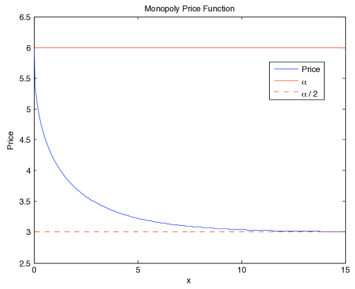
Figure 2: $p^{\star}_{M}(x)$ vs $x$ for $\sigma=0$

3.3 Small Degree of Substitutability Asymptotics under Deterministic Demand

We further analyze the non-stochastic (or ordinary) differential game ($\sigma_{1}=\sigma_{2}=0$) in which the monopoly problem is explicitly solvable, as in Proposition 3.1. We first note that $\gamma=0$ is equivalent to stating that firms have independent goods in the sense that they operate in markets without competing with one another. Hence, they have monopolies in their own markets, and it is clear that $V_{i}(x_{1},x_{2})=v_{M}(x_{i})$, where $v_{M}$ is the monopoly value function given in Eqn. (45). When $\gamma>0$, firms produce goods that are substitutable and are actually in competition with one another. We construct a perturbation expansion around the non-competitive case for small $\gamma>0$ to view the effects of a small amount of competition.

Recall our PDE system Eqn. (41), with $\mathcal{L}\equiv 0$. We look for an approximation to the solution of this system of PDEs of the form

$$V_{i}(x_{1},x_{2})=v_{M}(x_{i})+\gamma v_{i}^{(1)}(x_{1},x_{2})+\gamma^{2}v_{i}^{(2)}(x_{1},x_{2})+\cdots.$$ (46)

We use the static equilibrium price and demand functions that are given in Eqn. (27)-Eqn. (28), because we are working under the standing assumption that we have a Type $\langle$I$\rangle$ equilibrium. We first expand $S_{i}\left(\mathbf{x}\right)=s_{i}^{(0)}\left(\mathbf{x}\right)+\gamma s_{i}^{(1)}\left(\mathbf{x}\right)+\gamma^{2}s_{i}^{(2)}\left(\mathbf{x}\right)+\cdots$, where from Eqn. (40), we have

$$s_{i}^{(0)}=v_{M}^{\prime}(x_{i}),~{}~{}s_{i}^{(1)}=\frac{\partial v_{i}^{(1)}}{\partial x_{i}},~{}~{}s_{i}^{(2)}=\frac{\partial v_{i}^{(2)}}{\partial x_{i}}-\frac{1}{\beta}\frac{\partial v_{i}^{(1)}}{\partial x_{j}}.$$ (47)

Making use of Eqn. (26), the relevant expansions in powers of $\gamma$ are

$$p_{i}^{\star}(s_{1},s_{2}) = p_{M}^{\star}(s_{i}^{(0)})-\frac{\gamma}{2}D_{M}^{\star}(s_{j}^{(0)}+2\beta s_{i}^{(1)})-\frac{\gamma^{2}}{4\beta}D_{M}^{\star}(s_{i}^{(0)}+2\beta s_{j}^{(1)}+4\beta^{2}s_{i}^{(2)})+\cdots,$$ (48)

$$D_{i}^{\star}\left(s_{1},s_{2}\right) = D_{M}^{\star}(s_{i}^{(0)})-\frac{\gamma}{2\beta}D_{M}^{\star}(s_{j}^{(0)}-2\beta s_{i}^{(1)})-\frac{3\gamma^{2}}{4\beta^{2}}D_{M}^{\star}(s_{i}^{(0)}+\frac{2}{3}\beta s_{j}^{(1)}-\frac{4}{3}\beta^{2}s_{i}^{(2)})+\cdots,$$ (49)

$$D_{M}\left(p_{i}^{\star}\right) = D_{M}^{\star}(s_{i}^{(0)})+\frac{\gamma}{2\beta}D_{M}^{\star}(s_{j}^{(0)}+2\beta s_{j}^{(1)})+\frac{\gamma^{2}}{4\beta^{2}}D_{M}^{\star}(s_{i}^{(0)}+2\beta s_{j}^{(1)}+4\beta^{2}s_{i}^{(2)})+\cdots.$$ (50)

We define

$$q(x)\triangleq D_{M}^{\star}\left(v_{M}^{\prime}(x)\right)=\frac{1}{2\beta}\left(\alpha-v_{M}^{\prime}\left(x\right)\right).$$ (51)

Then, inserting Eqn. (46) into Eqn. (41), using Eqn. (48)-Eqn. (50), and comparing terms in $\gamma$ and $\gamma^{2}$, give that $v_{i}^{(1)}$ and $v_{i}^{(2)}$ satisfy

$$q(x_{1})\frac{\partial v^{(1)}_{i}}{\partial x_{1}}+q(x_{2})\frac{\partial v^{(1)}_{i}}{\partial x_{2}}+rv^{(1)}_{i} = -q(x_{1})q(x_{2}),$$ (52)

$$q(x_{1})\frac{\partial v_{i}^{(2)}}{\partial x_{1}}+q(x_{2})\frac{\partial v_{i}^{(2)}}{\partial x_{2}}+rv_{i}^{(2)} = \frac{1}{2\beta}\left(\frac{\partial v_{j}^{(1)}}{\partial x_{j}}+q(x_{i})\right)\cdot\left(\frac{\partial v_{i}^{(1)}}{\partial x_{j}}+q(x_{i})\right)$$ (53)

$$+\frac{1}{4\beta}\left(\frac{\partial v_{i}^{(1)}}{\partial x_{i}}+q(x_{j})\right)^{2}-\frac{3}{2\beta}\left(q(x_{i})\right)^{2},$$

for $i=1,2$ and $j\neq i$, with boundary conditions $v^{(1)}_{1}(x_{1},0)=v^{(2)}_{1}(x_{1},0)=0$ and $v^{(1)}_{1}(0,x_{2})=v^{(2)}_{1}(0,x_{2})=0$.

Proposition 3.2.

The solution $v_{i}^{(1)}$ is given, for $x_{1}>x_{2}$, by

$$v^{(1)}_{1}(x_{1},x_{2})=\frac{\alpha^{2}}{4\beta^{2}r}\left(e^{-rQ(x_{2})}\left(1+rQ(x_{2})\right)-e^{-rQ(x_{1})}\left(1-rQ(x_{2})\right)+e^{-r\left(Q(x_{1})+Q(x_{2})\right)}-1\right),$$ (54)

where

$$Q(x)\triangleq\int_{0}^{x}\frac{1}{q(u)}du=-\frac{1}{r}\log\left(-\mathbf{W}\left(-e^{-\mu x-1}\right)\right),$$ (55)

and, for $x_{2}\geq x_{1}$, by reversing the roles of $x_{1}$ and $x_{2}$ in Eqn. (54). The solution for $v^{(1)}_{2}$ is clearly the same, i.e. $v_{2}^{(1)}\equiv v_{1}^{(1)}$.

Proof.

The first step is to make the change of variables $(\xi,\eta)=\left(Q(x_{1}),Q(x_{2})\right)$ and $u(\xi,\eta)=e^{\frac{r}{2}\left(\xi+\eta\right)}v_{i}^{(1)}\left(Q^{-1}(\xi),Q^{-1}(\eta)\right)$ in Eqn. (52), which gives

$$\frac{\partial u}{\partial\xi}+\frac{\partial u}{\partial\eta}=f(\xi,\eta),\qquad\xi,\eta>0;\qquad u(\xi,0)=u(0,\eta)=0,$$ (56)

where $f(\xi,\eta)\triangleq-e^{\frac{r}{2}\left(\xi+\eta\right)}q\left(Q^{-1}(\xi)\right)q\left(Q^{-1}(\eta)\right).$ We see by the symmetry of this equation that $u(\xi,\eta)=u(\eta,\xi)$. We first suppose that $\xi>\eta$ and solve the PDE with the boundary condition $u(\xi,0)=0$. The other half of the solution can be obtained by symmetry. The solution is

$$u(\xi,\eta)=\int_{0}^{\eta}f(s+\xi-\eta,s)~{}ds=-\int_{0}^{\eta}e^{\frac{r}{2}(\xi-\eta+2s)}q\left(Q^{-1}\left(s+\xi-\eta\right)\right)q\left(Q^{-1}\left(s\right)\right)~{}ds.$$ (57)

By the definition of $q(x)$ in Eqn. (51) and $v_{M}$ in Eqn. (45), we have $q(x)=\frac{\alpha}{2\beta}\left[1+\mathbf{W}\left(-e^{-\mu x-1}\right)\right]$. This leads to Eqn. (55) since the range of $\mathbf{W}\left(-e^{-\mu x-1}\right)$ is $(-1,0)$. From properties of the Lambert $\mathbf{W}$ function, it follows easily that $-e^{-rs}=\mathbf{W}\left(-e^{-\mu Q^{-1}(s)-1}\right)$, and hence

$$q\left(Q^{-1}(s)\right)=\frac{\alpha}{2\beta}\left(1+\mathbf{W}\left(-e^{-\mu Q^{-1}(s)-1}\right)\right)=\frac{\alpha}{2\beta}\left(1-e^{-rs}\right).$$ (58)

We can now easily compute the integral in Eqn. (57). After restoring the transformations, we obtain Eqn. (54). ∎

Remark 3.1.

It can be verified by direct computation that the solutions $v_{i}^{(1)}$ in Proposition 3.2 are $\mathcal{C}^{1}$ on the line $x_{1}=x_{2}$. One can also solve the PDEs in Eqn. (53) to obtain a second-order correction for the value functions. We present this solution in Appendix B.

Remark 3.2.

While we do not give a formal convergence proof for the asymptotic approximation, we note that, since $v_{i}^{(1)}$ and $v_{i}^{(2)}$ are bounded with bounded continuous first-derivatives, the error terms $E_{i}$ defined by $V_{i}=v_{M}+\gamma v_{i}^{(1)}+\gamma^{2}v_{i}^{(2)}+E_{i}$ solve

$$q(x_{1})\frac{\partial E_{i}}{\partial x_{1}}+q(x_{2})\frac{\partial E_{i}}{\partial x_{2}}+rE_{i}=O(\gamma^{3})$$

with $E_{i}(x_{1},0)=E_{i}(0,x_{2})=0$. It follows from here that, for fixed $x_{1},x_{2}>0$, $|E_{i}(x_{1},x_{2})|=O(\gamma^{3})$ as $\gamma\downarrow 0$.

3.4 Discussion of Asymptotic Solution

We plot $v_{1}^{(1)}$ in Figure 33(a). Intuitively, it decreases from zero on the axes, because the first order correction decreases the value of the game due to the transition from a one-player monopoly to a two-player duopoly game. Hence, the greater the value of $\gamma$, the lower is the lifetime profit of an individual firm.

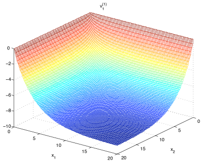
(a) $v_{1}^{(1)}$: Surface

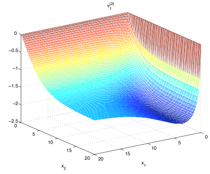
(b) $v_{1}^{(2)}$: Surface

Figure 3: $v_{1}^{(1)}$ and $v_{1}^{(2)}$. First- and second-order value function corrections.

We plot $v_{1}^{(2)}$ in Figure 33(b). It is again negative everywhere. Hence, the second-order correction serves to further decrease the value of the game from just the first-order approximation. We plot in Figure 4 the difference between $v_{1}^{(2)}$ and $v_{2}^{(2)}$. We do not make the same comparison for $v_{i}^{(1)}$ because $v_{1}^{(1)}-v_{2}^{(1)}\equiv 0$. We see from this figure that the sign of the difference is equal to the sign of $x_{1}-x_{2}$. Consider the situation in which Firm 1 has larger lifetime capacity, $x_{1}>x_{2}$. In the absence of competition, he has a larger value function, $v_{M}(x_{1})>v_{M}(x_{2})$. Introducing competition lowers his value by less than it lowers the value of the smaller firm. Therefore, competition serves to enhance the advantage of the larger firm. Of course, when two firms both have large remaining capacities, the inequality between firms does not have that much importance. It is only when one or both firms have small amounts of capacity remaining that inequalities across firms become magnified.

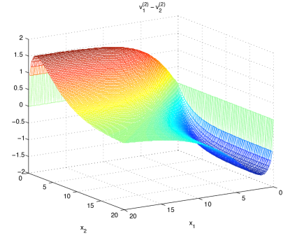
Figure 4: $v_{1}^{(2)}-v_{2}^{(2)}$. Difference between Firm 1 and Firm 2 second-order value function corrections.

For the remaining figures of this section we use the expansion up to order $\gamma$. We plot in Figure 55(a) the equilibrium price strategy of Firm 1 as a function of $x_{2}$ for various values of $\gamma$ using the first two terms of Eqn. (48). For $\gamma=0$, $\bar{p}_{1}^{\star}$ does not change with $x_{2}$ as the goods are independent. For increasing $\gamma$, as we would expect, the prices decrease at a faster rate as a function of $x_{2}$ because $\bar{p}_{1}^{\star}$ is more sensitive to the price of firm 2 when $\gamma$ is larger.

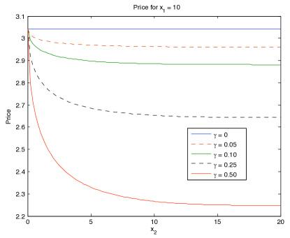
(a) Equilibrium price as a function of $x_{2}$ for $x_{1}=10$ fixed

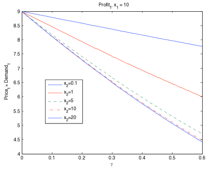
(b) $\bar{p}_{1}^{\star}\times D_{1}\left(\bar{p}_{1}^{\star},\bar{p}_{2}^{\star}\right)$ as a function of $\gamma$ for $x_{1}=10$

Figure 5: Equilibrium Price and Profit for Firm 1

In Figure 55(b), we plot the instantaneous profit for Firm 1, $\bar{p}_{1}^{\star}D_{1}(\bar{p}_{1}^{\star},\bar{p}_{2}^{\star})$. Each line shows the impact at a fixed $(x_{1},x_{2})$ of increasing $\gamma$, and we see from the slopes that the effect on reducing instantaneous profit is greater when $x_{2}$ is larger. Hence, competition, as measured by $\gamma$, only has bite when the competitor has comparable lifetime capacity levels.

Thus, when one considers the effect of competition on profit and prices, there are two main pieces of information one must take into account. The first is the degree of substitutability between goods. Fundamentally this means how similar is your good to your competitor’s. For example, one expects $\gamma$ to be large in the market for gasoline, because gas at one station is essentially the same as gas at a station across the street. The goods are not perfect substitutes because of travel costs, brand loyalty, and a host of other reasons. However, in the market for CDs, one expects a very low degree of substitutability, because an individual artist’s music is typically highly differentiated from that of another artist, even within a specific genre. It is reasonable to assume in such a market that $\gamma$ is quite low.

The second main piece of information is how credible is your competition. In this model, the proxy for a credible competitor is their level of lifetime capacity. If your competitor has very little lifetime capacity, then it stands to reason that regardless of how similar their good is to your own good, you will be a monopoly in short order. In contrast, if your competitor has a large amount of lifetime capacity, then they are a very credible threat to your business. As such, you must take such them very seriously even if their good is highly differentiated (but still substitutable) with your good. This can be seen in Figure 55(b) as even with $\gamma=0.1$, when $x_{2}$ is large relative to $x_{1}$, the instantaneous profit is much less than when $x_{2}$ is relatively small.

In Figure 6, we plot the solution to $\frac{dx_{1}}{dt}=-D_{1}\left(\bar{p}_{1}^{\star}(\mathbf{x}),\bar{p}_{2}^{\star}(\mathbf{x})\right)$, where we have used our expansion of order $\gamma$. We present the path of $x_{1}(t)$ over time for various different values of $\gamma$ starting from $x_{1}(0)=x_{2}(0)=10$. We see that as $\gamma$ increases, the time of the game increases. That is, it takes more time for Firm 1 to deplete their lifetime capacity when the degree of substitutability is greater.

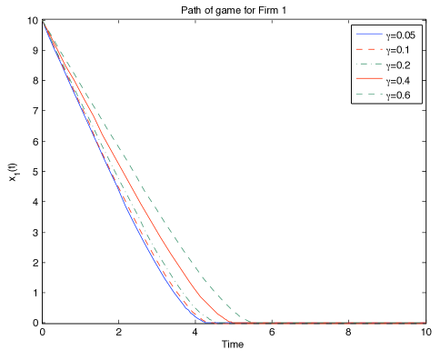
Figure 6: Path of Firm 1 Lifetime Capacity over time with $x_{1}(0)=x_{2}(0)=10$ for various values of $\gamma$

We can see this also by looking at the path of both demand and prices over the time of the game. These are plotted in Figures 7 7(a) and 7(b), respectively. We see that, for an individual firm, increasing the value of $\gamma$ drives down the price, while the demand first decreases and then increases. Common across all levels of $\gamma$, we see that as the capacity of the firm diminishes over time, the price increases while demand decreases.

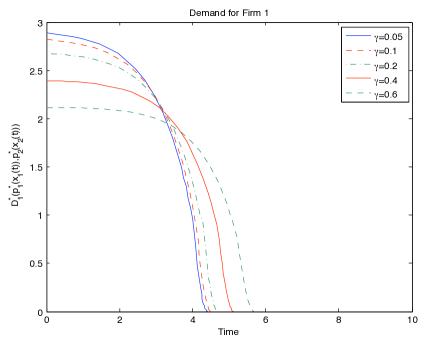
(a) Demand

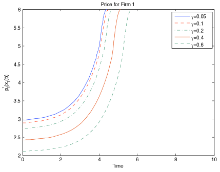
(b) Price

Figure 7: Path of Firm 1 Price and Demand over time with $x_{1}(0)=x_{2}(0)=10$ for various values of $\gamma$

Finally, we remark that one can confirm that the resulting demands from the asymptotic approximation for both firms are strictly positive in equilibrium. Therefore, our previous assumption on strictly positive demands is justified at least for $\gamma$ small enough.

4 Numerical Analysis

We have been able to capture many of the qualitative features of the model analytically in the case of deterministic demand using the asymptotic expansions of the previous section. However, in order to fully analyze the stochastic model we solve the full PDE system numerically. With these solutions, we then simulate paths of the game.

4.1 Finite Difference Solution of the PDE System

We employ fully implicit finite differences to find solutions $V_{1}$ and $V_{2}$ to the system in Eqn. (41). We can then use finite difference approximations to the derivatives of these value functions to obtain optimal price strategy functions and the resulting optimal demand functions. We use the parameter values $\alpha=6$, $\beta=1$, $r=1$, $\sigma_{1}=\sigma_{2}=0.6$ and $\rho=0.1$. The demands remain strictly positive for this choice of parameters and therefore, in this case, both firms are active participants in equilibrium.

For given levels of capacity $x_{1}$ and $x_{2}$, we define $\theta\triangleq\tan^{-1}\left(x_{2}/x_{1}\right)$. This is the angle in $(x_{1},x_{2})$ space that corresponds to the given capacity levels. We plot in Figure 8 8(a), the price of Firm 1 as a function of this $\theta$ for several values of $\gamma$. We also plot the optimal demand as a function of $\theta$ in Figure 8 8(b).

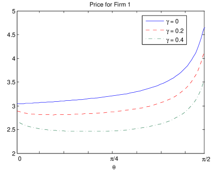
(a) Price

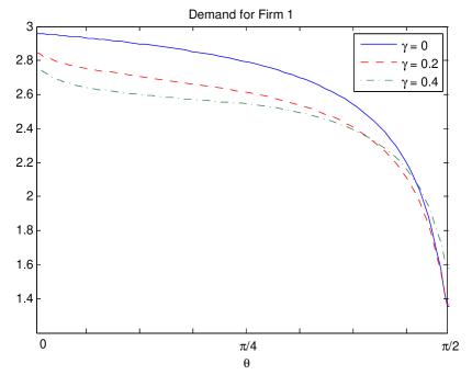
(b) Demand

Figure 8: Price and Demand for Firm 1 as a function of $\theta$ for various values of $\gamma$

These figures allow us to analyze price and demand effects for a fixed level of overall capacity in the market. At one end of the spectrum, $\theta=0$, we have that Firm 1 controls all of the capacity in the market. On the other end, $\theta=\pi/2$, Firm 2 controls all of the capacity. The price of Firm 1 decreases initially as $\theta$ increases, provided there is competition in the market, i.e. $\gamma>0$. However, the price starts to increase once $\theta$ moves beyond $\pi/4$ and Firm 1 holds the minority share of the available capacity in the market. Furthermore, price decreases at a greater rate for higher levels of $\gamma$. This implies that the optimal price strategies result in the lowest prices when substitutability is high, i.e. $\gamma$ is large, and when all firms in a market are of the same relative size, i.e. $\theta$ is close to $\pi/4$. Increasing the number of firms in a market, thereby increasing the level of competition, does not always have a large effect on consumer welfare. This is because if an additional firm enters a market with a small capacity when there already exist large capacity firms, then essentially this means they are not credible competitors to the large firms and therefore prices do not necessarily have to adjust by a large amount to account for this additional competition. On the other hand, we see from these figures, for a given fixed level of total market capacity, consumers are always better off if the capacity is spread evenly across firms, provided the firms produce substitute goods (i.e. $\gamma>0$). Consumers therefore face the best possible situation when there exist multiple firms in a market whose goods have a high degree of substitutability and whose relative sizes are the close to the same.

Figures 9 9(a) and 9(b) are the contours of the optimal price strategy for Firm 1 for two different values of $\gamma$. The strategy changes from charging a constant price as a function of $x_{2}$ when $\gamma=0$, to charging a price that is decreasing in $x_{2}$ for $\gamma=0.4$. This is as expected because prices should reflect the credibility of one’s competitor when that competitor produces a good which is substitutable with one’s own good. We see that although prices are decreasing in both $x_{1}$ and $x_{2}$, they decrease at a faster rate with respect to $x_{1}$.

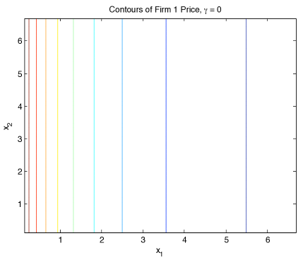
(a) $\gamma=0$

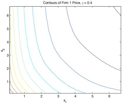
(b) $\gamma=0.4$

Figure 9: Contours of Firm 1 Price Strategy for $\gamma=0$ and $0.4$.

4.2 Game Simulations

We can use our numerical solution of the value functions to obtain numerical versions of the equilibrium prices, $\bar{p}_{i}^{\star}(\mathbf{x}(t))$. These in turn can be used to obtain numerical versions of the equilibrium capacity trajectories over time by making use of Eqn. (34), i.e.

$$dx_{i}(t)=-D_{i}\left(\bar{p}_{1}^{\star}(x_{1}(t),x_{2}(t)),\bar{p}_{2}^{\star}(x_{1}(t),x_{2}(t))\right)~{}dt+\sigma_{i}~{}dW_{i}(t),\hskip 14.22636pti=1,2.$$

We simulate paths of the Brownian motions in order to obtain paths of the game over time. We present an example of these paths in Figure 1010(a) for $\gamma=0.4$. This is just one example but it displays many features of the game. Here we started both firms with an initial capacity of $x_{1}(0)=x_{2}(0)=10$. Over time these decrease, but because of the stochastic component of demand, we see that at any given moment in time, we cannot say with certainty which firm will necessarily have a higher level of capacity. In this example, initially Firm 2 gains an advantage, however we see as time progresses that Firm 2 runs out of capacity before Firm 1, and hence for a period of time Firm 1 has a monopoly.

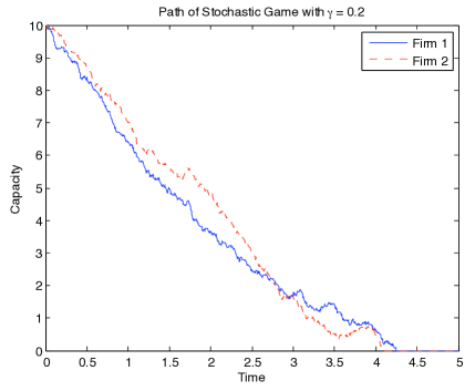
(a) Path of Stochastic Game for both firms with $\gamma=0.3$

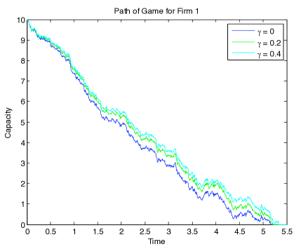
(b) Paths of game for firm 1 for varying $\gamma$

Figure 10: Path of Stochastic Game

For a fixed realization of the Brownian path, we plot in Figure 1010(b), the path of the capacity for Firm 1 for various values of $\gamma$. We see that as $\gamma$ increases, the time until the capacity of Firm 1 is exhausted, also appears to increase. This effect, where increased competition prolongs the lifetime of firms, is consistent with what we saw in Figure 6 in the deterministic game.

5 Conclusion

We have studied nonzero-sum stochastic differential games arising from Bertrand competitions, in particular, the case of a duopoly with linear demand functions. By considering the case where there is a small degree of substitutability between the firms’ goods, we are able to construct an asymptotic approximation that captures many of the qualitative features of the ordinary differential game. Numerical solutions further provide insight into the stochastic case and where there is a higher degree of substitutability. In our study of the dynamic game, we concentrated on the case where both firms have positive demand in equilibrium. As we saw in the static game, it is possible for there to arise cases where this does not occur. However, the study of such cases remains an interesting open question in the analysis of these dynamic Bertrand games.

These tools allow us to quantify the effects of substitutability and relative firm size on prices, demands and profits. In particular, we find that consumers benefit the most when a market is structured with many firms of the same relative size producing highly substitutable goods. However, a large degree of substitutability does not always lead to large drops in price, for example when two firms have a large difference in their size. That is, consumers benefit the most when firms are competing with other firms whom they deem to be credible threats. A competitor is a credible threat only if they have capacity large enough to match their competitors. For example, the existence of a very small coffee shop does not greatly affect the pricing decisions of Starbucks.

It is of interest to extend the analysis here to markets with nonlinear demand systems as well as to random demand environments. By the latter, we mean that baseline demand and substitutability may vary stochastically over time with economic conditions or consumer tastes. For example, in the linear demand system Eqn. (2), there may be fluctuations in the intercept parameter $A$, which is a measure of the general level of demand due to business cycles and recessions, or in $C/B$, which is the measure of substitutability, as certain brands fall out of fashion, for example what Toyota is experiencing in 2010. Finally, an important related direction is to connect, in a probabilistic way, prices to the mechanism of customer arrival, for example, by making the arrival intensity a function of prices. Such models have been used in a variety of applications for the single-player price setting problem. However, their use in competitive markets leads to multi-player stochastic differential games with jumps, and is a direction we are currently pursuing.

Appendix A Proof of Proposition 2.2

We have assumed that $\hat{p}_{N}$ exists. We show that this implies $\hat{p}_{N-1}$ exists. The result for all $n$ will then follow by induction. Fix $p_{1},\ldots,p_{N-2}$ and denote this vector of prices by $\rho$. Let $p_{N-1}$ be an arbitrary price. We denote $\hat{p}_{N}(\rho,p_{N-1})$ by $\tilde{p}$. We then have two cases, depending on $p_{N-1}$, under which we wish to show $D_{N-1}^{N-1}\left(\rho,p_{N-1}\right)<0$. The first case is $p_{N-1}>\hat{p}_{N}(\rho,\tilde{p})$, which implies

$$D^{N-1}_{N-1}\left(\rho,p_{N-1}\right)=D^{N}_{N-1}\left(\rho,p_{N-1},\tilde{p}\right)=D^{N}_{N}\left(\rho,\tilde{p},p_{N-1}\right)<D^{N}_{N}\left(\rho,\tilde{p},\hat{p}\left(\rho,\tilde{p}\right)\right)=0.$$

The second case we must consider is the reverse inequality, i.e. $p_{N-1}<\hat{p}_{N}(\rho,\tilde{p})$. This implies

$$0=D^{N}_{N}\left(\rho,p_{N-1},\tilde{p}\right)>D^{N}_{N}\left(\rho,\hat{p}\left(\rho,\tilde{p}\right),\tilde{p}\right)=D^{N}_{N-1}\left(\rho,\tilde{p},\hat{p}\left(\rho,\tilde{p}\right)\right)=D^{N-1}_{N-1}\left(\rho,\tilde{p}\right).$$

Hence, regardless of the relative size of $p_{N-1}$ and $\hat{p}_{N}\left(\rho,\tilde{p}\right)$, we have that $D^{N-1}_{N-1}(p)$ is negative for some vector of prices $p$. We have ignored the case $p_{N-1}=\hat{p}_{N}(\rho,\tilde{p})$, because this would change the above inequalities to equalities and we would have the choke price we are looking for.

We know by Assumption 2.4 that $D^{N-1}_{N-1}$ is a decreasing function of $p_{N-1}$. We have shown above that there exists some vector of prices $p$ such that $D^{N-1}_{N-1}(p)<0$. We thus need only show that there exists some vector of prices $p$ where $D^{N-1}_{N-1}(p)>0$. This will establish the existence of the choke price.

Fix some vector of prices $\bar{p}=\left(p_{1},\ldots,p_{N-2},0\right)$, where $p_{1},\ldots,p_{N-2}$ are arbitrary prices. Denote by $\underline{0}$ the vector in $\mathbb{R}^{N-1}$ of all zeros. Recall that $D^{N}_{N}\left(\underline{0},0\right)>D^{N}_{N}\left(\underline{0},\hat{p}_{N}\left(\underline{0}\right)\right)=0$. This implies $\hat{p}_{N}\left(\underline{0}\right)>0$. We then have

$$D^{N-1}_{N-1}\left(\bar{p}\right)=D^{N}_{N-1}\left(\bar{p},\hat{p}_{N}\left(\bar{p}\right)\right)\geq D^{N}_{N-1}\left(\bar{p},\hat{p}_{N}\left(\underline{0}\right)\right)>D^{N}_{N-1}\left(\bar{p},0\right)\geq D^{N}_{N-1}\left(\underline{0},0\right)=D^{N}_{N}\left(\underline{0},0\right)>0.$$

Hence, for the vector $\bar{p}$ we have that $D^{N-1}_{N-1}(\bar{p})$ is positive. Therefore, there must exist some $\hat{p}_{N-1}$ for every set of prices $p_{1},\ldots,p_{N-2}$ such that $D^{N-1}_{N-1}\left(p_{1},\ldots,p_{N-2},\hat{p}_{N-1}\right)=0$.

Appendix B Second-order approximation

We give the solution of the PDEs Eqn. (53) for $v_{i}^{(2)}$. Using the solution to $v_{i}^{(1)}$ found in Proposition 3.2, making the same change of variables $(\xi,\eta)=\left(Q(x_{1}),Q(x_{2})\right)$ and solving leads to

$$v_{1}^{(2)} = \frac{\alpha^{2}}{8\beta^{3}}e^{-rQ(x_{2})}\left[-\frac{Q(x_{2})^{2}}{2}\left(\frac{2re^{rQ(x_{2})}}{e^{rQ(x_{2})}-1}+\frac{r\varphi_{1}}{1-e^{-rQ(x_{1})}}\right)-\frac{Q(x_{2})(1-\varphi_{1})}{1-e^{-rQ(x_{1})}}\right.$$ (59)

$$\left.+\frac{3}{2r}\left(e^{rQ(x_{2})}-1\right)-\frac{\left(1-\varphi_{1}\right)^{2}}{2r\left(e^{rQ(x_{2})}\left(1-e^{-rQ(x_{1})}\right)\right)}+\frac{1-\varphi_{1}}{2r}\right.$$

$$\left.-\frac{3}{r}\left(e^{rQ(x_{2})}-\varphi_{1}^{2}e^{-rQ(x_{2})}-1+\varphi_{1}^{2}-2\varphi_{1}rQ(x_{2})\right)\right].$$

for $x_{1}>x_{2}$ where $\varphi_{1}=\exp\left\{-r\left(Q(x_{1})-Q(x_{2})\right)\right\}$. For $x_{2}>x_{1}$,

$$v_{1}^{(2)} = \frac{\alpha^{2}}{8\beta^{3}}e^{-rQ(x_{1})}\left[-\frac{Q(x_{1})^{2}}{2}\left(\frac{re^{rQ(x_{1})}}{e^{rQ(x_{1})}-1}+\frac{2r\varphi_{2}}{1-e^{-rQ(x_{2})}}\right)-\frac{2Q(x_{1})(1-\varphi_{2})}{1-e^{-rQ(x_{2})}}\right.$$ (60)

$$\left.+\frac{3}{2r}\left(e^{rQ(x_{1})}-1\right)-\frac{(1-\varphi_{2})^{2}}{re^{rQ(x_{1})}\left(1-e^{-rQ(x_{2})}\right)}+\frac{1-\varphi_{2}}{r}\right.$$

$$\left.-\frac{3}{r}\left(e^{rQ(x_{1})}-2rQ(x_{1})-e^{-rQ(x_{1})}\right)\right].$$

where $\varphi_{2}=\exp\left\{-r\left(Q(x_{2})-Q(x_{1})\right)\right\}$. We omit the details of this lengthy calculation.

Appendix C $N$-player Stochastic Differential Game with Linear Demands

Consider the $N$-player dynamic Bertrand game under the linear demand system introduced in Section 3. Within this section we explicitly assume that all firms participate in equilibrium, i.e. all firms receive positive demand. In the language of Section 2, this would mean that the resulting dynamic equilibrium is of Type $\langle$I$\rangle$. Let $V_{i}(\mathbf{x})$ denote the value functions defined by the $N$-player analog of Eqn. (36). Then, the associated PDE system, analog of Eqn. (37), is

$$\mathcal{L}V_{i}+\sup_{p_{i}\geq 0}\left\{-\sum_{k=1}^{N}D^{N}_{k}(p)\frac{\partial V_{i}}{\partial x_{k}}+p_{i}D^{N}_{i}(p)\right\}-rV_{i}=0,~{}~{}i=1,\ldots,N,$$ (61)

where we explicitly denote the dependence of the demand functions on $N$ to indicate the size of the vector $p$ in the argument. Here,

$$\mathcal{L}=\frac{1}{2}\sum_{i=1}^{N}\sum_{j=1}^{N}\Sigma_{ij}\frac{\partial^{2}V_{i}}{\partial x_{i}\partial x_{j}},$$ (62)

where $\left(\Sigma_{ij}\right)_{i,j=1,\ldots,N}$ is the covariance matrix between the Brownian motions in Eqn. (34).

For a fixed $i$, we note that we can write

$$D^{N}_{j}(p) = -\frac{C}{B}D^{N}_{i}(p)+A\left(1+\frac{C}{B}\right)-B\left(1-\frac{C^{2}}{B^{2}}\right)p_{j}+C\left(1+\frac{C}{B}\right)\underset{k\neq i}{\sum_{k\neq j}}p_{k}$$ (63)

$$= -\frac{C}{B}D^{N}_{i}(p)+D^{N-1}_{\pi_{i}(j)}\left(p_{-i}\right),$$

where $p_{-i}=p\backslash\{p_{i}\}$ and

$$\pi_{i}(k)=\left\{\begin{array}[]{ccl}k,&&k<i\\ k-1,&&k>i.\end{array}\right.$$ (64)

This decomposition means that one can represent a firm’s demand function at the level $N$ as a linear combination of another given firm’s demand function at the level $N$ and their own demand function at the level $N-1$ with the given firm being removed. This is a consequence of the consistency of demand functions and the existence of choke prices.

Hence, using this decomposition, we have, for $i=1,\ldots,N$

$$\mathcal{L}V_{i}-\sum_{k\neq i}^{N}D^{N-1}_{\pi_{i}(k)}(p_{-i})\frac{\partial V_{i}}{\partial x_{k}}+\sup_{p_{i}\geq 0}\left\{D^{N}_{i}(p)\left(p_{i}-\frac{\partial V_{i}}{\partial x_{i}}+\frac{C}{B}\sum_{k\neq i}\frac{\partial V_{i}}{\partial x_{k}}\right)\right\}-rV_{i}=0.$$ (65)

Therefore, we can use the results of the static Bertrand game to write the PDEs as

$$\mathcal{L}V_{i}-\sum_{k\neq i}^{N}D^{N-1}_{\pi_{i}(k)}(p^{\star}_{-i})\frac{\partial V_{i}}{\partial x_{k}}+G_{i}^{N}\left(s_{1},\ldots,s_{N}\right)=rV_{i}$$ (66)

where the prices $p^{\star}$ are the solutions of the $N$-player static game with costs

$$S_{i}(\mathbf{x})=\frac{\partial V_{i}}{\partial x_{i}}-\frac{C}{B}\sum_{k\neq i}\frac{\partial V_{i}}{\partial x_{k}},\qquad i=1,\ldots,N$$ (67)

and with corresponding profit functions $G_{i}^{N}\left(s_{1},\ldots,s_{N}\right)=D^{N}_{i}(p^{\star})\left(p^{\star}_{i}-s_{i}\right)$.

The boundary conditions for this PDE depends on the PDEs that result by considering a market with $N-1$ firms. That is, on any edge of an orthant where $x_{i}=0$ and $x_{j}>0$ for all $j\neq i$, we have $V_{i}\equiv 0$ and that $V_{j}$ solve the same PDE problem except where firm $i$ is removed and thus there are $N-1$ firms in the market. This is similar to the duopoly problem where the boundary condition depends on the monopoly problem. The remaining conditions can be worked out in a similar fashion.

References

- Arrow et al. [1951] K. J. Arrow, T. Harris, and J. Marschak. Optimal Inventory Policy. Econometrica, 19(3):250–272, 1951.
- Başar and Olsder [1995] T. Başar and G. J. Olsder. Dynamic Noncooperative Game Theory. Academic Press, 2nd edition, 1995.
- Bather [1966] J. A. Bather. A Continuous Time Inventory Model. Journal of Applied Probability, 3(2):538–549, 1966.
- Bensoussan and Frehse [2002] A. Bensoussan and J. Frehse. Regularity results for nonlinear elliptic systems and applications. Springer, 2002.
- Bensoussan and Frehse [1984] A. Bensoussan and J. Frehse. Nonlinear elliptic systems in stochastic game theory. Journal für die Reine und Angewandte Mathematik, 8(Band 350):24–67, 1984.
- Bensoussan et al. [2009] A. Bensoussan, D. Diltz, and C. Ho. Real options in Stackelberg games with an arithmetic Brownian motion cash flow process. Preprint, University of Texas at Dallas, 2009.
- Bertrand [1883] J. Bertrand. Théorie mathématique de la richesse sociale. Journal des Savants, 67:499–508, 1883.
- Besbes and Zeevi [2009] O. Besbes and A. Zeevi. Dynamic Pricing Without Knowing the Demand Function: Risk Bounds and Near-Optimal Algorithms. Operations Research, 57(6):1407–1420, 2009.
- Björk and Murgoci [2008] T. Björk and A. Murgoci. A General Theory of Markovian Time Inconsistent Stochastic Control Problems. Preprint. Stockholm School of Economics, September 2008.
- Chamberlin [1933] E. Chamberlin. The Theory of Monopolistic Competition. Harvard University Press, Cambridge, MA, 1933.
- Cournot [1838] A. Cournot. Recherches sur les Principes Mathématique de la Théorie des Richesses. Hachette, Paris, 1838. English translation by N.T. Bacon, published in Economic Classics, Macmillan, 1897, and reprinted in 1960 by Augustus M. Kelley.
- d’Aspremont et al. [1979] C. d’Aspremont, J. Gamszewicz, and J.-F. Thisse. On Hotelling’s “Stability in Competition”. Econometrica, 47(5):1145–1150, 1979.
- Dockner et al. [2000] E. Dockner, S. Jørgensen, N. v. Long, and G. Sorger. Differential games in economics and management science. Cambridge University Press, 2000.
- Ekeland and Pirvu [2008] I. Ekeland and T. A. Pirvu. Investment and consumption without commitment. Preprint. University of British Columbia, February 2008.
- Engwerda [2005] J. C. Engwerda. LQ Dynamic Optimization and Differential Games. John Wiley & Sons, 2005.
- Fleming and Souganidis [1989] W. Fleming and P. Souganidis. On the existence of value functions of two-player, zero-sum stochastic differential games. Indiana University Mathematics Journal, 38:293–314, 1989.
- Friedman [1971] A. Friedman. Differential Games. John Wiley & Sons, 1971. Reprinted by Dover, 2006.
- Friedman [1983] J. Friedman. Oligopoly Theory. Cambridge University Press, 1983.
- Fudenberg and Tirole [1991] D. Fudenberg and J. Tirole. Game Theory. MIT Press, 1991.
- Hamadène [1998] S. Hamadène. Backward-forward SDE’s and stochastic differential games. Stochastic Processes and their Applications, 77:1–15, 1998.
- Hamadène and Zhang [2010] S. Hamadène and J. Zhang. The continuous time nonzero-sum Dynkin game problem and application in game options. SIAM J. Control Optim., 48(5):3659–3669, 2010.
- Harris et al. [2010] C. Harris, S. Howison, and R. Sircar. Games with exhaustible resources. SIAM J. Applied Mathematics, 2010. To appear.
- Hotelling [1929] H. Hotelling. Stability in competition. The Economic Journal, 39(153):41–57, 1929.
- Jun and Vives [2004] B. Jun and X. Vives. Strategic incentives in dynamic duopoly. Journal of Economic Theory, 116:249–281, 2004.
- Lasry and Lions [2007] J.-M. Lasry and P.-L. Lions. Mean field games. Japanese Journal of Mathematics, 2(1):229–260, March 2007.
- Mas-Colell et al. [1995] A. Mas-Colell, M. D. Whinston, and J. R. Green. Microeconomic Theory. Oxford University Press, New York, New York, 1995.
- Vives [1999] X. Vives. Oligopoly pricing: old ideas and new tools. MIT Press, Cambridge, MA, 1999.