Contribution to hadrons’ width from classical instability of Y configuration
and other string hadron models

Abstract

We consider various hadron models with a string carrying $n=3$ massive points (quarks): Y configuration, linear baryon model $q$-$q$-$q$ and the closed string. For these models classical rotational states (planar uniform rotations) are tested for stability with respect to small disturbances. It is shown that rotations of all mentioned models are unstable, but nature of this instability is different. For the model Y the instability results from existence of multiple real frequencies in the spectrum of small disturbances, but for the linear model and the closed string the similar spectra contain complex frequencies, corresponding to exponentially growing modes of disturbances. This classical rotational instability is important for describing excited hadrons, in particular, for the linear model and the closed string it results in additional contribution in width of hadron states.

I Introduction

In various string models of hadrons material points representing quarks are connected by the Nambu-Goto strings (relativistic strings) simulating strong interaction between quarks at large distances Nambu ; Ch ; AY ; 4B ; Ko ; lin ; PY ; PRTr ; InSh ; Solovm ; stab ; Y02 (Fig. 1). This string has linearly growing energy (energy density is equal to the string tension $\gamma$), describes contribution of the gluon field, QCD confinement mechanism and quasilinear Regge trajectories for excited states of mesons and baryons 4B ; Ko ; lin ; PY ; PRTr ; InSh ; Solovm .

Such a string with massive ends in Fig. 1a may be regarded as the meson string model Ch . String models of the baryon were suggested in the following four topologically different variants AY : (b) the quark-diquark model $q$-$qq$ Ko $\big{[}$on the classic level it coincides with the meson model (a)$\big{]}$, (c) the linear configuration $q$-$q$-$q$ lin , (d) the “three-string” model or Y configuration AY ; PY , and (e) the “triangle” model or $\Delta$ configuration PRTr . String models of the glueball Solovgl ; EstrCBRS ; ZayasS ; glY08 were considered in the variants in Fig. 1f – i. Here massive points describe valent gluons.

One should choose the most preferable model among the mentioned four string baryon models in Fig. 1b – e. The problem of this choice remains open 4B ; Ko ; lin ; PY ; PRTr ; InSh ; Solovm ; stab ; Y02 . Different models have different advantages. In particular, rotational states (planar uniform rotations) of all mentioned baryon models generate linear or quasilinear Regge trajectories, but with different slopes $\alpha^{\prime}$ 4B ; Ko . For the baryon models in Fig. 1b and c like for the meson model in Fig. 1a this slope and the string tension $\gamma$ are connected by the Nambu relation Nambu $\alpha^{\prime}=1/(2\pi\gamma)$. The experimental value of this slope $\alpha^{\prime}\simeq 0{.}9$ GeV^-2 is equal for both meson and baryon Regge trajectories. So it is the argument in favour of these two baryon models.

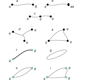
Figure 1: String models of mesons, baryons and glueballs

For rotational states of the linear baryon configuration (Fig. 1c) the middle mass is at the rotational center. In papers lin ; stab we have shown in numerical experiments that the mentioned states are unstable with respect to small disturbances and in Ref. Unst09 we proved this result analytically.

The string baryon model Y (Fig. 1d) for its rotational states demonstrates Regge trajectories with the slope PY $\alpha^{\prime}=1/(3\pi\gamma)$. To obtain $\alpha^{\prime}\simeq 0{.}9$ GeV^-2 we are to assume that the effective string tension $\gamma_{Y}$ in this model differs from $\gamma$ in models in Figs. 1a – c (the fundamental string tension) and equals $\gamma_{Y}=\frac{2}{3}\gamma$ 4B ; InSh . Moreover, rotations of the Y string configuration are also unstable with respect to small disturbances on the classic level stab ; Y02 . But specific features of this instability require more profound investigation: in Sect. III of this paper we study difference in character of rotational instability for Y and linear configurations.

The string baryon model “triangle” or $\Delta$ generates a set of rotational states with different topology PRTr . The so called triangle states was applied for describing excited baryon states on the Regge trajectories 4B ; InSh , but in this case (like for the model Y) we are to take another effective string tension $\gamma_{\Delta}=\frac{3}{8}\gamma$.

Different string models shown in Fig. 1f – i were used for describing glueballs (bound states of gluons) and other exotic hadrons Solovgl ; EstrCBRS ; ZayasS ; glY08 predicted in QCD. String models of glueballs include the open string with enhanced tension $\gamma_{adj}=\frac{9}{4}\gamma$ (the adjoint string) and two constituent gluons at the ends EstrCBRS ; Bali0 in Fig. 1f; the closed string without masses (Fig. 1g) Solovgl ; ZayasS ; MeyerT and the closed string carrying massive points (Fig. 1h and i) glY08 .

The problem of stability for rotations with respect to small disturbances is very important for choosing the most adequate string model for baryons or glueballs 4B ; stab ; Y02 ; glY08 . Note that instability of classical rotations for some string configuration does not mean that the considered string model must be totally prohibited. All excited hadron states (objects of modelling) are resonances, they are unstable with respect to strong decays. So they have rather large width $\Gamma$. On the level of string models these decays are described as string breaking with probability, proportional to the string length $\ell$ Kodecay ; GuptaR . The corresponding width $\Gamma=\Gamma_{br}\sim\ell$.

If classical rotations of a string configuration are unstable, this instability gives the additional contribution $\Gamma_{inst}$ to width $\Gamma$. This effect is one of manifestations of rotational instability. It can restrict applicability of some string models, if the total width $\Gamma$ predicted by this model (below we suppose $\Gamma=\Gamma_{br}+\Gamma_{inst}$) essentially exceeds experimental data.

The stability problem for rotational states is solved for the string with massive ends (Fig. 1a, b). Analytical investigation of small disturbances demonstrated that rotational states of this system are stable, and there is the spectrum of quasirotational states in the linear vicinity of these stable rotations stab ; qrottmf .

For string baryon models $q$-$q$-$q$, Y and $\Delta$ evolution of small disturbances of rotational states was investigated in numerical experiments stab ; Y02 . These calculations demonstrated instability of rotations for the linear model and for the Y-configuration. However, we are to estimate analytically increments of instability for all models and to investigate its influence on properties of excited hadrons.

In this paper dynamics of the mentioned string models is described in Sect. II. In Sections III and IV for the models Y and $q$-$q$-$q$ correspondingly (Figs. 1d and c) small disturbances of rotations are studied analytically and increments of instability are calculated. In Sect. V the similar result is presented for central rotational states (with a massive point at the rotational center) of the closed string (Fig. 1e, h or i). In Sect. VI we study how rotational instability enlarges width of excited hadrons on Regge trajectories.

II Dynamics of a string with massive points

Dynamics of an open or closed string carrying $n$ point-like masses $m_{1},\dots,m_{n}$ is determined by the action PRTr ; glY08

$$A=-\gamma\int\limits_{D}\sqrt{-g}\;d\tau d\sigma-\sum\limits_{j=1}^{n}m_{j}\int\sqrt{\dot{x}_{j}^{2}(\tau)}\;d\tau.$$ (1)

Here $\gamma$ is the string tension, $g$ is the determinant of the induced metric $g_{ab}=\eta_{\mu\nu}\partial_{a}X^{\mu}\partial_{b}X^{\nu}$ on the string world surface $X^{\mu}(\tau,\sigma)$ embedded in Minkowski space $R^{1,3}$, $\eta_{\mu\nu}=\mbox{diag}(1,-1.-1,-1)$, the speed of light $c=1$.

A world surface of the closed string mapping into $R^{1,3}$ from the domain

$$D=\big{\{}(\tau,\sigma):\,\tau\in R,\;\sigma_{0}(\tau)<\sigma<\sigma_{n}(\tau)\big{\}}$$

is divided into $n$ world sheets by the world lines of massive points

$$x_{j}^{\mu}(\tau)=X^{\mu}(\tau,\sigma_{j}(\tau)),\quad j=0,1,\dots,n.$$

Two of these functions $x_{0}(\tau)$ and $x_{n}(\tau)$ describe the same trajectory of the $n$-th massive point, and their equality forms the closure condition

$$X^{\mu}(\tau,\sigma_{0}(\tau))=X^{\mu}(\tau^{*},\sigma_{n}(\tau^{*}))$$ (2)

on the tube-like world surface PRTr ; MilSh . These equations may contain two different parameters $\tau$ and $\tau^{*}$, connected via the relation $\tau^{*}=\tau^{*}(\tau)$. This relation should be included in the closure condition (2).

For the string baryon model $q$-$q$-$q$ (an open string with $n=3$ masses) the domain $D$ in Eq. (1) has the form $\sigma_{1}(\tau)<\sigma<\sigma_{3}(\tau)$. This domain and the world surface are divided into two sheets by the line $\sigma=\sigma_{2}(\tau)$. Naturally, there is no closure condition in this model.

Equations of motion for both open and closed strings with massive points result from the action (1) and its variation. If we use invariance of the action (1) with respect to nondegenerate reparametrizations $\tau=\tau(\tilde{\tau},\tilde{\sigma})$, $\sigma=\sigma(\tilde{\tau},\tilde{\sigma})$ and choose the coordinates $\tau$, $\sigma$ satisfying the orthonormality conditions on the world surface

$$(\partial_{\tau}X\pm\partial_{\sigma}X)^{2}=0,$$ (3)

the equations of motion are reduced to the simplest form 4B ; PRTr . They include the string motion equation

$$\frac{\partial^{2}X^{\mu}}{\partial\tau^{2}}-\frac{\partial^{2}X^{\mu}}{\partial\sigma^{2}}=0,$$ (4)

and equations for two types of massive points: for endpoints of the model $q$-$q$-$q$

$$m_{1}\frac{d}{d\tau}\frac{\dot{x}_{1}^{\mu}(\tau)}{\sqrt{\dot{x}_{1}^{2}(\tau)}}-\gamma\bigl{[}X^{{}^{\prime}\!\mu}+\dot{\sigma}_{1}(\tau)\,\dot{X}^{\mu}\bigr{]}\bigg{|}_{\sigma=\sigma_{1}} = 0,\qquad$$ (5)

$$m_{3}\frac{d}{d\tau}\frac{\dot{x}_{3}^{\mu}(\tau)}{\sqrt{\dot{x}_{3}^{2}(\tau)}}+\gamma\bigl{[}X^{{}^{\prime}\!\mu}+\dot{\sigma}_{3}(\tau)\,\dot{X}^{\mu}\bigr{]}\bigg{|}_{\sigma=\sigma_{3}} = 0;\qquad$$ (6)

and for the middle point in the mentioned model or points on a closed string

$$m_{j}\frac{d}{d\tau}\frac{\dot{x}_{j}^{\mu}(\tau)}{\sqrt{\dot{x}_{j}^{2}(\tau)}}+\gamma\Big{[}X^{{}^{\prime}\!\mu}+\dot{\sigma}_{j}(\tau)\dot{X}^{\mu}\Big{]}\Big{|}_{\sigma=\sigma_{j}-0}$$

$${}-\gamma\Big{[}X^{{}^{\prime}\!\mu}+\dot{\sigma}_{j}(\tau)\dot{X}^{\mu}\Big{]}\Big{|}_{\sigma=\sigma_{j}+0}=0,$$ (7)

$$m_{n}\frac{d}{d\tau}\frac{\dot{x}_{0}^{\mu}(\tau)}{\sqrt{\dot{x}_{0}^{2}(\tau)}}+\gamma\big{[}X^{{}^{\prime}\!\mu}(\tau^{*},\sigma_{n})-X^{{}^{\prime}\!\mu}(\tau,0)\big{]}=0.$$ (8)

Here $\dot{X}^{\mu}\equiv\partial_{\tau}X^{\mu}$, $X^{{}^{\prime}\!\mu}\equiv\partial_{\sigma}X^{\mu}$, the scalar product $(\xi,\zeta)=\eta_{\mu\nu}\xi^{\mu}\zeta^{\nu}$.

In Eq. (8) for $n$-th massive point we fix

$$\sigma_{0}(\tau)=0,\qquad\sigma_{n}(\tau)=2\pi$$ (9)

without loss of generality with the help of substitutions $\tau\pm\sigma=f_{\pm}(\tilde{\tau}\pm\tilde{\sigma})$, keeping conditions (3) (conformal flatness of the induced metric $g_{ab}$) PRTr ; MilSh .

For the open string model $q$-$q$-$q$ we can fix the similar conditions at the ends lin ; 4B in Eqs. (5), (6):

$$\sigma_{1}(\tau)=0,\qquad\sigma_{3}(\tau)=\pi.$$ (10)

For the string baryon model Y (Fig. 1d) three world sheets (swept up by three string segments) are parametrized with three different functions $X_{j}^{\mu}(\tau_{j},\sigma)$ stab ; Y02 . Here we use different notations $\tau_{1}$, $\tau_{2}$, $\tau_{3}$ for “time-like” parameters and the same symbol $\sigma$ for “space-like” parameters. These three world sheets are joined along the world line of the junction that may be set as $\sigma=0$ for all sheets without loss of generality, so the action of this configuration takes the form stab ; Y02

$$A=-\sum_{j=1}^{3}\int d\tau_{j}\bigg{[}\gamma\!\!\int\limits_{0}^{\sigma_{j}(\tau_{j})}\!\!\sqrt{-g_{j}}\,d\sigma+m_{j}\sqrt{\dot{x}_{j}^{2}(\tau_{j})}\,\bigg{]}.$$ (11)

Here $g_{j}=\dot{X}_{j}^{2}X_{j}^{{}^{\prime}\!2}-(\dot{X}_{j},X_{j}^{{}^{\prime}})^{2}$, $\dot{x}_{j}^{\mu}(\tau_{j})=\frac{d}{d\tau_{j}}X^{\mu}(\tau_{j},\sigma_{j})$, $\dot{X}_{j}^{\mu}=\partial_{\tau_{j}}X_{j}^{\mu}$, other notations are the same.

At the junction of three world sheets $X_{j}^{\mu}(\tau_{j},\sigma)$ the parameters $\tau_{j}$ are connected as follows Y02

$$\tau_{2}=\tau_{2}(\tau),\quad\tau_{3}=\tau_{3}(\tau),\quad\tau_{1}\equiv\tau.$$

So the condition in the junction takes the form

$$X_{1}^{\mu}\big{(}\tau,0\big{)}=X_{2}^{\mu}\big{(}\tau_{2}(\tau),0\big{)}=X_{3}^{\mu}\big{(}\tau_{3}(\tau),0\big{)}.$$ (12)

Dynamical equations for the Y configuration result from the action (11) and under the orthonormality conditions (3)

$$(\partial_{\tau_{j}}X_{j}\pm\partial_{\sigma}X_{j})^{2}=0,\qquad j=1,2,3$$

and condition (10) $0\leq\sigma\leq\pi$ on three world sheets take the form Y02

$$\frac{\partial^{2}X_{j}^{\mu}}{\partial\tau_{j}^{2}}-\frac{\partial^{2}X_{j}^{\mu}}{\partial\sigma^{2}}=0,$$ (13)

$$\sum_{j=1}^{3}X_{j}^{{}^{\prime}\!\mu}\big{(}\tau_{j}(\tau),0\big{)}\,\dot{\tau}_{j}(\tau)=0,$$ (14)

$$m_{j}\frac{dU^{\mu}_{j}(\tau_{j})}{d\tau_{j}}+\gamma X_{j}^{{}^{\prime}\!\mu}(\tau_{j},\pi)=0.$$ (15)

Here $\dot{\tau}_{j}=\frac{d}{d\tau}\tau_{j}(\tau)$,

$$U^{\mu}_{j}(\tau_{j})=\frac{\dot{x}^{\mu}_{j}(\tau_{j})}{\sqrt{\dot{x}^{2}_{j}(\tau_{j})}}.$$ (16)

Equations (12) – (15) describe all motions of the Y configuration like Eqs. (2) – (4), (7), (8) for the closed string with masses and Eqs. (3) – (6), (7) ($j=2$) for the string baryon model $q$-$q$-$q$.

III Rotational stability for Y configuration

Rotational states of the Y configuration (Fig. 1d) correspond to planar uniform rotation of three rectangular string segments connected at the junction at angles of $120^{\circ}$ 4B ; Ko ; PY . These states may be parametrized as Y02

$$\underline{X}_{j}^{\mu}(\tau_{j},\sigma)=\Omega^{-1}\big{[}\omega\tau_{j}e_{0}^{\mu}+\sin(\omega\sigma)\cdot e^{\mu}(\tau_{j}+\Delta_{j})\big{]}.$$ (17)

Here $\tau_{1}=\tau_{2}=\tau_{3}$, $e_{0},\,e_{1},\,e_{2},\,e_{3}$ is the orthonormal tetrade in Minkowski space $R^{1,3}$, $\Delta_{j}=2\pi(j-1)/(3\omega)$,

$$e^{\mu}(\tau)=e_{1}^{\mu}\cos\omega\tau+e_{2}^{\mu}\sin\omega\tau$$ (18)

is the unit space-like rotating vector directed along the first string segment. Below we consider the case Y02

$$m_{1}=m_{2}=m_{3},\qquad v_{1}=v_{2}=v_{3}$$ (19)

Expression (17) satisfies Eq. (13) and conditions (3), (12), (14), (15), if angular velocity $\Omega$, the value $\omega$, constant velocities $v_{j}$ of the massive points are connected by the relations 4B

$$v_{j}=\sin(\pi\omega)=\left[\Big{(}\frac{\Omega m_{j}}{2\gamma}\Big{)}^{2}+1\right]^{1/2}-\frac{\Omega m_{j}}{2\gamma}.$$ (20)

In Refs. stab ; Y02 we demonstrated in numerical experiments, that rotational states (17) of the Y configuration are unstable with respect to small disturbances. Here we solve this problem analytically.

Let us consider a slightly disturbed motion of this configuration with a world surface $X_{j}^{\mu}(\tau_{j},\sigma)$ close to the surface $\underline{X}_{j}^{\mu}(\tau_{j},\sigma)$ of the rotational state (17) (below we underline values, describing rotational states). This disturbed motion is described by the general solution of Eq. (13)

$$X_{j}^{\mu}(\tau_{j},\sigma)=\frac{1}{2}\bigl{[}\Psi^{\mu}_{j+}(\tau_{j}+\sigma)+\Psi^{\mu}_{j-}(\tau_{j}-\sigma)\bigr{]},$$ (21)

for every world sheet. Functions $\Psi^{\mu}_{j\pm}(\tau)$ have isotropic derivatives

$$\dot{\Psi}_{j+}^{2}=\dot{\Psi}_{j-}^{2}=0.$$ (22)

as a consequence of the orthonormality conditions (3).

If we substitute Eq. (21) into conditions (12), (14) and (15), they may be reduced to the form Y02

$$\Psi^{\mu}_{1+}(\tau)+\Psi^{\mu}_{1-}(\tau)=\Psi^{\mu}_{j+}(\tau_{j})+\Psi^{\mu}_{j-}(\tau_{j}),$$ (23)

$$\sum\limits_{j=1}^{3}\big{[}\dot{\Psi}^{\mu}_{j+}(\tau_{j})-\dot{\Psi}^{\mu}_{j-}(\tau_{j})\big{]}\dot{\tau}_{j}(\tau)=0,$$ (24)

$$\displaystyle\dot{\Psi}_{j\pm}^{\mu}(\tau_{j}\pm\pi)=\frac{m_{j}}{\gamma}\Big{[}\sqrt{-\dot{U}_{j}^{2}(\tau_{j})}\,U_{j}^{\mu}(\tau_{j})\mp\dot{U}_{j}^{\mu}(\tau_{j})\Big{]}.\quad$$ (25)

If we know velocities $U_{j}^{\mu}(\tau_{j})$ of massive ends, we can calculate functions $X_{j}^{\mu}(\tau_{j},\sigma)$ for world sheets via equations (25) and (21). So we search velocities $U_{j}^{\mu}$ for disturbed motion as small corrections to vectors $\underline{U}_{j}^{\mu}$ for rotational states (17):

$$U_{j}^{\mu}(\tau_{j})=\underline{U}_{j}^{\mu}(\tau_{j})+u_{j}^{\mu}(\tau_{j}).$$ (26)

We suppose disturbances $u_{j}^{\mu}(\tau_{j})$ to be small ($|u_{j}^{\mu}|\ll 1$), so we omit squares of $u_{j}^{\mu}$ when we substitute the expression (26) into equalities $U_{j}^{2}=\underline{U}_{j}^{2}=1$, resulting in relations

$$\big{(}\underline{U}_{j}(\tau_{j}),u_{j}(\tau_{j})\big{)}=0,$$ (27)

and into dynamical equations (23) – (25).

The vectors $\underline{U}_{j}^{\mu}$ for rotational states (17) in Eq. (26) are

$$\underline{U}_{j}^{\mu}(\tau_{j})=(1-v_{j}^{2})^{-1/2}\big{[}e_{0}^{\mu}+v_{j}\acute{e}^{\mu}(\tau_{j}+\Delta_{j})\big{]},$$ (28)

where rotating vector

$$\acute{e}^{\mu}(\tau)=-e_{1}^{\mu}\sin(\omega\tau)+e_{2}^{\mu}\cos(\omega\tau),$$

is orthogonal to the vector (18).

We suppose that for a disturbed motions the “time” parameters

$$\tau_{j}(\tau)=\tau+\delta_{j}(\tau),\quad j=2,3,\quad|\delta_{j}(\tau)|\ll 1,$$ (29)

have small deviations $\delta_{2}(\tau)$ and $\delta_{3}(\tau)$ from $\tau\equiv\tau_{1}$.

When we substitute disturbances (26) and (29) into expressions (25) and equations (23) and (24) at the junction’s world line, we get identities for rotational terms (28) and (in the linear approximation with respect to $u_{j}^{\mu}$, $\delta_{j}$) the following system of vector equations for these disturbances:

$$\begin{array}[]{c}\makebox[170.71652pt]{$\sum\limits_{\pm}\Big{[}Qu_{1}^{\mu}(\pm)\pm\dot{u}_{1}^{\mu}(\pm)+\underline{U}_{1}^{\mu}(\pm)\big{(}e(\pm),\dot{u}_{1}(\pm)\big{)}\Big{]}=$}\\ \makebox[170.71652pt]{$=\sum\limits_{\pm}\Big{\{}Qu_{j}^{\mu}(\pm)\pm\dot{u}_{j}^{\mu}(\pm)+\underline{U}_{j}^{\mu}(\pm)\big{(}e(\pm_{j}),\dot{u}_{j}(\pm)\big{)}+$}\\ \displaystyle+\frac{\gamma}{m_{1}}\Big{[}\dot{\delta}_{j}(\tau)\dot{\underline{\Psi}}_{j\pm}^{\mu}(\tau)+\delta_{j}(\tau)\ddot{\underline{\Psi}}_{j\pm}^{\mu}(\tau)\Big{]}\Big{\}},\\ \displaystyle\sum\limits_{j=1}^{3}\sum\limits_{\pm}\Big{\{}\mp\frac{\gamma}{m_{1}}\Big{[}\dot{\delta}_{j}\dot{\underline{\Psi}}_{j\pm}^{\mu}(\tau)+\delta_{j}\ddot{\underline{\Psi}}_{j\pm}^{\mu}(\tau)\Big{]}+\\ \makebox[170.71652pt]{$+\dot{u}_{j}^{\mu}(\pm)\pm Qu_{j}^{\mu}(\pm)\pm\underline{U}_{j}(\pm)\big{(}e(\pm_{j}),\dot{u}_{j}(\pm)\big{)}\Big{\}}=0.$}\end{array}$$ (30)

Here $(\pm)\equiv(\tau\pm\pi)$, $(\pm_{j})\equiv(\tau\pm\pi+\Delta_{j})$, functions

$$\dot{\underline{\Psi}}_{j\pm}^{\mu}(\tau)=\frac{m_{1}Q}{\gamma c_{1}}\big{[}e_{0}^{\mu}+v_{1}\acute{e}^{\mu}(\mp_{j})\pm c_{1}e^{\mu}(\mp_{j})\big{]}$$ (31)

correspond to rotational state (17),

$$Q=\omega v_{1}/c_{1},\qquad c_{1}=\cos(\pi\omega)=\sqrt{1-v_{1}^{2}}.$$ (32)

One should add Eqs. (27) to the system (30).

The similar equations in Ref. Y02 were deduced with the following mistake in corrections, connected with the “times” (29):

$$\dot{\underline{\Psi}}_{j\pm}^{\mu}(\tau_{j})\simeq\dot{\underline{\Psi}}_{j\pm}^{\mu}(\tau)+\ddot{\underline{\Psi}}_{j\pm}^{\mu}(\tau)\cdot\delta_{j}(\tau).$$

In particular, for vectors (18) this correction doesn’t reduce to the substitution $\tau\to\tau+{}$const made in Ref. Y02 in the expression $e^{\mu}(\tau_{j})\simeq e^{\mu}(\tau)+\omega\acute{e}^{\mu}(\tau)\cdot\delta_{j}(\tau)$. This correction has the following true form:

$$e^{\mu}(\tau_{j}\mp\pi+\Delta_{j})\simeq e^{\mu}(\tau\mp\pi+\Delta_{j})+\omega\acute{e}^{\mu}(\mp_{j})\cdot\delta_{j}(\tau).$$ (33)

In Ref. Y02 we search solutions of the system (30) in the form

$$u_{j}^{\mu}(\tau) = \big{[}A_{j}^{0}e_{0}^{\mu}+A_{j}^{z}e_{3}^{\mu}+c_{1}A_{j}e^{\mu}(\tau+\Delta_{j})+{}$$ (34)

$$+ v_{1}^{-1}A_{j}^{0}\acute{e}^{\mu}(\tau+\Delta_{j})\big{]}\exp(-i\xi\tau),$$

$$\delta_{j}(\tau) = \delta_{j}\exp(-i\xi\tau),\quad j=2,3$$ (35)

with small complex amplitudes $A_{j}^{0}$, $A_{j}$, $A_{j}^{z}$, $\delta_{j}$. Projections of these equations onto basis vectors $e_{0}^{\mu}$, $e^{\mu}(\tau)$, $\acute{e}^{\mu}(\tau)$, $e_{3}^{\mu}$ form the system of algebraic equations with respect to these amplitudes. Here the expression (34) satisfy conditions (27) due to the factor $v_{1}^{-1}A_{j}^{0}$ at $\acute{e}^{\mu}$.

Projections of the mentioned equations onto the vector $e_{3}^{\mu}$ are

$$\begin{array}[]{c}(\xi\tilde{c}+Q\tilde{s})(A_{1}^{z}+A_{2}^{z}+A_{3}^{z})=0,\\ (\xi\tilde{s}-Q\tilde{c})(A_{1}^{z}-A_{j}^{z})=0,\quad j=2,3.\rule{0.0pt}{13.99995pt}\end{array}$$

They don’t depend on corrections of the type (33). Here

$$\tilde{c}=\cos\pi\xi,\qquad\tilde{s}=\sin\pi\xi.$$

In Ref. Y02 we obtained solutions of these equations, describing 2 types of small oscillations of rotating Y configuration (in $e_{3}$-direction). Corresponding frequencies $\xi$ of these oscillations are roots of the equations

$$\xi/Q=\cot\pi\xi,\qquad\xi/Q=-\tan\pi\xi.$$ (36)

All roots of Eqs. (36) are simple roots and real numbers, therefore amplitudes of such fluctuations do not grow with growing time $t$.

Small disturbances in the rotational ($e_{1},e_{2}$) plane are described by the system of 9 linear equations with 8 unknown values $A_{j}^{0}$, $A_{j}$, $\delta_{j}$. These equations are projections (scalar products) of the system (30) onto 3 vectors $e_{0}$, $e(\tau)$, $\acute{e}(\tau)$. Eight independent equations among them are reduced to the form:

$$\begin{array}[]{c}Q_{c}(A_{j}^{0}-A_{1}^{0})+i\xi\tilde{c}(A_{j}-A_{1})=i\xi D_{j},\\ 2(\xi\tilde{s}A_{1}-iQ_{s}A_{1}^{0})=(iQ_{s}+\epsilon_{j}\omega_{c})A_{j}^{0}-(\xi+i\epsilon_{j}\omega)\tilde{s}A_{j},\rule{0.0pt}{11.99998pt}\\ 2(\omega_{c}A_{1}^{0}-i\omega\tilde{s}A_{1})=(iQ_{s}\epsilon_{j}-\omega_{c})A_{j}^{0}+(i\omega-\epsilon_{j}\xi)A_{j},\rule{0.0pt}{11.99998pt}\\ iQ_{s}(A_{1}^{0}+A_{2}^{0}+A_{3}^{0})=\xi\tilde{s}(A_{1}+A_{2}+A_{3}),\rule{0.0pt}{11.99998pt}\\ 2(Q_{c}A_{1}^{0}+i\xi\tilde{c}A_{1})=\rule{0.0pt}{11.99998pt}\\ =\sum\limits_{j=2}^{3}\Big{[}(Q_{c}+i\epsilon_{j}\omega_{s})A_{j}^{0}+(i\xi-\epsilon_{j}\omega)(\tilde{c}A_{j}-D_{j})\Big{]},\\ 2(i\omega_{s}A_{1}^{0}-\omega\tilde{c}A_{1})=\rule{0.0pt}{11.99998pt}\\ =\sum\limits_{j=2}^{3}\Big{[}(i\omega_{s}-\epsilon_{j}Q_{c})A_{j}^{0}-(i\epsilon_{j}\xi+\omega)(\tilde{c}A_{j}-D_{j})\Big{]}.\end{array}$$ (37)

Here $\epsilon_{j}=(-1)^{j}\sqrt{3}$, $D_{j}=\delta_{j}Q/c_{1}$, $j=2,3$,

$$\begin{array}[]{c}Q_{c}=Q(1+v_{1}^{-2})\tilde{c}-\xi\tilde{s},\quad Q_{s}=Q(1+v_{1}^{-2})\tilde{s}+\xi\tilde{c},\\ \omega_{c}=\omega\tilde{c}-\xi c_{1}v_{1}^{-1}\tilde{s},\quad\omega_{s}=\omega\tilde{s}+\xi c_{1}v_{1}^{-1}\tilde{c}.\end{array}$$

Nontrivial solutions of this system exist if and only if its determinant equals zero. This equality after simplification is reduced to the following equation:

$$(\xi^{2}-\omega^{2})(\omega Q_{c}-\xi\omega_{s})(\omega Q_{s}+\xi\omega_{c})=0.$$ (38)

It is equivalent to equalities $\xi=\pm\omega$ and two equations

$$\frac{\xi^{2}-q}{2Q\xi}=-\tan\pi\xi,\qquad\frac{\xi^{2}-q}{2Q\xi}=\cot\pi\xi.$$ (39)

Here $q=Q^{2}(1+v_{1}^{-2})=\omega^{2}(1+v_{1}^{2})/(1-v_{1}^{2})$.

Analysis of roots for equations (38), (39) for complex values $\xi=\xi_{1}+i\xi_{2}$ is presented in Fig. 2, where the thick and thin lines are correspondingly zero level lines of the real and imaginary part of the l.h.s. of Eq. (38) $f(\xi)=f(\xi_{1}+i\xi_{2})$. Roots of this equation are shown as cross points of a thick line with a thin line.

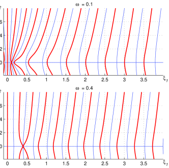
Figure 2: Zero level lines for real (thick and) and imaginary part(thin) of Eq. (38) for specified values $\omega$

Fig. 2 shows that for values $\omega=0{.}1$ and $\omega=0{.}4$, corresponding to $v_{1}\simeq 0.309$ and $v_{1}\simeq 0.951$, all roots of Eq. (38) are real numbers and form a countable set. The same behavior takes place for all values $\omega\in(0,1/2)$, that is for all rotations (17) with equal masses (19).

If a spectrum of small disturbances contains complex frequencies $\xi=\xi_{1}+i\xi_{2}$, exponentially growing modes $|u_{j}|\sim e^{\xi_{2}\tau}$ appear. Such a spectrum for rotations (17) of the model Y doesn’t contain complex frequencies. So instability of rotational states (17), observer in numerical experiments stab ; Y02 , has other nature.

This instability results from existence of double roots $\xi=\pm\omega$ in Eq. (38). If we take $\xi=\pm\omega$ not only the first factor in Eq. (38), but also the second factor $(\omega Q_{c}-\xi\omega_{s})$ vanishes. This fact is seen in Fig. 2 and may be proved, if we consider the first Eq. (39) and Eqs. (20), (32).

Double roots of Eq. (38) may correspond to oscillatory modes with linearly growing amplitude. To analyze this effect for the frequency $\xi=\omega$ we substitute small disturbances

$$\begin{array}[]{c}\!\!\!u_{j}^{\mu}(\tau)=\Big{\{}(A_{j}^{0}+\tilde{A}_{j}^{0}\tau)\big{[}e_{0}^{\mu}+v_{1}^{-1}\acute{e}^{\mu}(\tau+\Delta_{j})\big{]}+\!\!\!\!\\ +(A_{j}+\tilde{A}_{j}\tau)\,c_{1}e^{\mu}(\tau+\Delta_{j})\Big{\}}\exp(-i\omega\tau),\\ \delta_{j}(\tau)=(D_{j}+\tilde{D}_{j}\tau)\,c_{1}Q^{-1}\exp(-i\omega\tau)\end{array}$$ (40)

in the system (30) for expressions (34) and (35). This results after transformation in the following system

$$\begin{array}[]{c}\tilde{A}_{1}^{0}=\tilde{A}_{2}^{0}=\tilde{A}_{3}^{0}=0,\\ \tilde{A}_{j}=\frac{1}{2}(i\epsilon_{j}-1)\tilde{A}_{1},\quad\tilde{D}_{j}=\frac{1}{2}c_{1}(i\epsilon_{j}-3)\tilde{A}_{1},\rule{0.0pt}{13.99995pt}\\ 2A_{j}^{0}=iv_{1}c_{1}\omega^{-1}\epsilon_{j}\tilde{A}_{1}-(i\epsilon_{j}+1)A_{1}^{0},\rule{0.0pt}{13.99995pt}\\ \makebox[170.71652pt]{$\quad 2A_{j}+(1-i\epsilon_{j})A_{1}=\frac{i}{v_{1}c_{1}}\big{[}2A_{j}^{0}+(1-i\epsilon_{j})A_{1}^{0}\big{]},\rule{0.0pt}{16.00008pt}$}\\ 2D_{j}=(3i+\epsilon_{j})(\pi v_{1}\tilde{A}_{1}+v_{1}^{-1}A_{1}^{0}+ic_{1}A_{1}^{0}),\rule{0.0pt}{13.99995pt}\end{array}$$ (41)

with respect to complex amplitudes in (40) (here $j=2,3$). It is analog of Eqs. (37).

The algebraic system (41) has a family of nontrivial solutions specified with an arbitrary nonzero value of the complex constant $\tilde{A}_{1}$. These solutions describe disturbances (40) of the rotational states with linearly growing amplitude:

$$|u_{j}^{\mu}|\simeq|\tilde{A}_{1}|c_{1}\tau\qquad|\delta_{j}|\simeq\sqrt{3}c_{1}^{2}Q_{1}^{-1}|\tilde{A}_{1}|\tau.$$ (42)

This modes let us to conclude, that rotational states (17) of the string model Y with $m_{1}=m_{2}=m_{3}$ are unstable, because an arbitrary small disturbance contains linearly growing modes of the type (42) in its spectrum.

In papers Y02 ; stab we investigated numerically disturbed rotational states of the string configuration Y and observed instability of the states (17). Small disturbances grew and resulted in transformation of the Y-shaped three-string into the linear $q$-$q$-$q$ configuration after merging a massive point with the junction.

Numerical experiments demonstrate that evolution of small disturbances for velocities $U_{j}^{\mu}$ or values $\tau_{j}(\tau)$ corresponds to expression (42), amplitudes of disturbances linearly grow and frequency of oscillations (with respect to $\tau$) is equal $\omega$. Omitting details of numerical modelling for motions close to rotations (17) (described in Refs. Y02 ; stab ), we demonstrate in Fig. 3 dependence of deviations $\tau_{2}(\tau)-\tau$ (solid line) and $\tau_{3}(\tau)-\tau$ (dashed line) on the time parameter $\tau$ for disturbed rotational states (17). Here we test the state with masses (19) for $\omega=0.1$ and with the initial disturbance of the component $\dot{\Psi}_{1\pm}^{1}(\tau)$ less than 0.01 of its value (31).

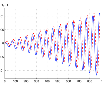
Figure 3: Dependence of $\tau_{2}(\tau)-\tau$ (solid line) and $\tau_{3}(\tau)-\tau$ (dashed line) on $\tau$ for disturbed rotational state

Instability of rotational states (17) with linearly growing amplitudes takes place also in the limit $m_{j}\to 0$, or, it is equivalent, $v_{j}\to 1$.

IV Rotational states and their stability for linear model

Rotational states of the linear string model $q$-$q$-$q$ are planar uniform rotations of the rectilinear string segment with the middle quark at the rotational center. These rotations may be described by the following exact solution of equations (3) – (7) stab :

$$\underline{X}^{\mu}(\tau,\sigma)=\Omega^{-1}\big{[}\omega\tau e_{0}^{\mu}+\cos(\omega\sigma+\phi_{1})\cdot e^{\mu}(\tau)\big{]},$$ (43)

Here $\sigma\in[0,\pi]$, $\Omega$ is the angular velocity, $e^{\mu}(\tau)$ is the unit space-like rotating vector (18) directed along the string. Values $\omega$ (dimensionless frequency) and $\phi_{1}$ are connected with the constant speeds $v_{j}$ of the ends

$$v_{1}=\cos\phi_{1},\;\;\;v_{3}=-\cos(\pi\omega+\phi_{1}),\;\;\;\frac{m_{j}\Omega}{\gamma}=\frac{1-v_{j}^{2}}{v_{j}},$$ (44)

where $j=1,3$. The central massive point of the $q$-$q$-$q$ system is at rest (in the corresponding frame of reference) at the rotational center. Its inner coordinate is

$$\sigma_{2}(\tau)=\underline{\sigma}_{2}=\frac{\pi-2\phi_{1}}{2\omega}={\mbox{const}}.$$ (45)

Rotational states (43) of the model $q$-$q$-$q$ was tested for stability in Ref. stab in numerical experiments and in Ref. Unst09 analytically. These experiments and calculations demonstrated instability (growth of small disturbances). Here we use analytical approach applied in Refs. qrottmf ; Unst09 for testing stability of the states (43).

Let us consider a slightly disturbed motion of the system $q$-$q$-$q$ in the linear vicinity of the rotational state (43). This disturbed motion is described by the general solution (21) of Eq. (4)

$$X^{\mu}(\tau,\sigma)=\frac{1}{2}\big{[}\Psi^{\mu}_{j+}(\tau+\sigma)+\Psi^{\mu}_{j-}(\tau-\sigma)\big{]}.$$ (46)

Here $j=1$ for $\sigma\in[0,\sigma_{2}]$ and $j=2$ for $\sigma\in[\sigma_{2},\pi]$, functions $\Psi^{\mu}_{j\pm}(\tau)$ have isotropic derivatives (22) due to the orthonormality conditions (3). The functions $\Psi^{\mu}_{j\pm}$ are smooth, the world surface (46) (smooth if $\sigma\neq\sigma_{2}$) is continuous at the line $\sigma=\sigma_{2}(\tau)$. This condition in terms Eq. (46) takes the form

$$\Psi^{\mu}_{1+}(+_{2})+\Psi^{\mu}_{1-}(-_{2})=\Psi^{\mu}_{2+}(+_{2})+\Psi^{\mu}_{2-}(-_{2}),$$ (47)

where $(\pm_{2})\equiv\big{(}\tau\pm\sigma_{2}(\tau)\big{)}$.

We use underlined symbols for describing the particular exact solution (43) for the rotational states. For example, we denote

$$\underline{\Psi}^{\mu}_{1\pm}(\tau)=\underline{\Psi}^{\mu}_{2\pm}(\tau)=\Omega^{-1}\big{[}e_{0}^{\mu}\omega\tau+e^{\mu}(\tau\pm\phi_{1}/\omega)\big{]}$$ (48)

the functions in Eq. (46) corresponding to the states (43): $\underline{X}^{\mu}=\frac{1}{2}\big{[}\underline{\Psi}^{\mu}_{j+}(\tau+\sigma)+\underline{\Psi}^{\mu}_{j-}(\tau-\sigma)\big{]}$.

To describe any small disturbances of the rotational motion, that is motions close to states (43) we consider vector functions $\Psi^{\mu}_{j\pm}$ close to $\underline{\Psi}^{\mu}_{j\pm}$ (48) in the form

$$\Psi^{\mu}_{j\pm}(\tau)=\underline{\Psi}^{\mu}_{j\pm}(\tau)+\psi_{j\pm}^{\mu}(\tau).$$ (49)

Disturbances $\psi_{j\pm}^{\mu}(\tau)$ are supposed to be small, so we omit squares of $\psi_{j\pm}$ when we substitute the expression (49) into dynamical equations (5) – (7) and (47). In other words, we work in the first linear vicinity of the states (43). Both functions $\dot{\Psi}^{\mu}_{j\pm}$ and $\dot{\underline{\Psi}}^{\mu}_{j\pm}$ in expression (49) must satisfy the condition (22) resulting from Eq. (3), hence in the first order approximation on $\dot{\psi}_{j\pm}$ the following scalar product equals zero:

$$\big{(}\underline{\dot{\Psi}}_{j\pm},\dot{\psi}_{j\pm}\big{)}=0.$$ (50)

For disturbed (quasirotational) motions of the model $q$-$q$-$q$ the inner coordinate $\sigma_{2}(\tau)$ of the middle massive point differs from the constant value $\underline{\sigma}_{2}$ (45) and should include the following small correction $\delta_{2}$:

$$\sigma_{2}(\tau)=\underline{\sigma}_{2}+\delta_{2}(\tau).$$ (51)

If we substitute expressions (49), (51) with (46) into the continuity condition (47) and three equations (5), (6), (7) (with $j=2$) for massive points, we obtain equalities for summands with $\underline{\Psi}^{\mu}_{j\pm}$ and four equations for small disturbances $\psi_{j\pm}^{\mu}(\tau)$ in the first linear approximation:

$$\begin{array}[]{c}\psi_{1+}^{\mu}(+_{2})+\psi_{1-}^{\mu}(-_{2})=\psi_{2+}^{\mu}(+_{2})+\psi_{2-}^{\mu}(-_{2}),\\ \dot{\psi}_{1+}^{\mu}+\dot{\psi}_{1-}^{\mu}-\underline{U}_{1}^{\mu}\big{(}\underline{U}_{1},\dot{\psi}_{1+}^{\mu}+\dot{\psi}_{1-}^{\mu}\big{)}=Q_{1}\big{(}\psi_{1+}^{\mu}-\psi_{1-}^{\mu}\big{)},\rule{0.0pt}{11.99998pt}\\ \dot{\psi}_{2+}^{\mu}(+)+\dot{\psi}_{2-}^{\mu}(-)-\underline{U}_{3}^{\mu}\big{(}\underline{U}_{3},\dot{\psi}_{2+}^{\mu}(+)+\dot{\psi}_{2-}^{\mu}(+)\big{)}\rule{0.0pt}{11.99998pt}\\ =Q_{3}\big{[}\psi_{2-}^{\mu}(-)-\psi_{2+}^{\mu}(+)\big{]},\rule{0.0pt}{11.99998pt}\\ \dot{\psi}_{1+}^{\mu}(+_{2})+\dot{\psi}_{1-}^{\mu}(-_{2})-2a_{0}\big{[}\dot{\delta}_{2}e^{\mu}(\tau)+\omega\delta_{2}\acute{e}^{\mu}(\tau)\big{]}\rule{0.0pt}{11.99998pt}\\ \displaystyle=\frac{e_{0}^{\mu}}{2a_{0}}\Big{[}\big{(}\dot{\underline{\Psi}}_{1+}(+_{2}),\dot{\psi}_{1-}(-_{2})\big{)}+\big{(}\dot{\underline{\Psi}}_{1-}(-_{2}),\dot{\psi}_{1+}(+_{2})\big{)}\Big{]}\rule{0.0pt}{16.99998pt}\\ +2Q_{2}\big{[}\psi_{2+}^{\mu}(+_{2})-\psi_{1+}^{\mu}(+_{2})\big{]}.\rule{0.0pt}{11.99998pt}\end{array}$$ (52)

Here

$$Q_{j}=\frac{\gamma}{m_{j}}\sqrt{\underline{\dot{x}}_{j}^{2}(\tau)}=\frac{\gamma a_{0}}{m_{j}}\sqrt{1-v_{j}^{2}},\quad a_{0}=\frac{\omega}{\Omega},$$ (53)

vector-functions similar to (28)

$$\underline{U}_{j}^{\mu}(\tau)=(1-v_{j}^{2})^{-1/2}\big{[}e_{0}^{\mu}-\epsilon_{j}v_{j}\acute{e}^{\mu}(\tau)\big{]},\quad\epsilon_{1}=-1,\quad\epsilon_{3}=1,$$

are unit velocity vectors of the moving massive points.

If we consider projections (scalar products) of 4 equations (52) onto 4 basic vectors $e_{0}$, $e(\tau)$, $\acute{e}(\tau)$, $e_{3}$ and add Eqs. (50) we obtain the system of 20 differential equations with deviating arguments with respect to 17 unknown functions: $\delta_{2}(\tau)$ and 16 projections

$$\begin{array}[]{c}\psi_{j\pm}^{0}\equiv(e_{0},\psi_{j\pm}),\quad\psi_{j\pm}^{3}\equiv(e_{3},\psi_{j\pm}),\\ \psi_{j\pm}\equiv(e,\psi_{j\pm}),\quad\acute{\psi}_{j\pm}\equiv(\acute{e},\psi_{j\pm});\rule{0.0pt}{11.99998pt}\end{array}$$ (54)

Four projections of Eqs. (52) onto direction $e_{3}$ (orthogonal to the rotational plane $e_{1}$, $e_{2}$) form the closed subsystem with respect to 4 functions (54) $\psi_{j\pm}^{3}$:

$$\!\!\begin{array}[]{c}\psi_{1+}^{3}(+_{2})+\psi_{1-}^{3}(-_{2})=\psi_{2+}^{3}(+_{2})+\psi_{2-}^{3}(-_{2}),\\ \dot{\psi}_{1+}^{3}(\tau)+\dot{\psi}_{1-}^{3}(\tau)=Q_{1}\big{[}\psi_{1+}^{3}(\tau)-\psi_{1-}^{3}(\tau)\big{]},\rule{0.0pt}{11.99998pt}\\ \dot{\psi}_{2+}^{3}(+)+\dot{\psi}_{2-}^{3}(-)=Q_{3}\big{[}\psi_{2-}^{3}(-)-\psi_{2+}^{3}(+)\big{]},\rule{0.0pt}{11.99998pt}\\ \dot{\psi}_{1+}^{3}(+_{2})+\dot{\psi}_{1-}^{3}(-_{2})=2Q_{2}\big{[}\psi_{2+}^{3}(+_{2})-\psi_{1+}^{3}(+_{2})\big{]}.\rule{0.0pt}{11.99998pt}\end{array}\!\!\!\!\!$$ (55)

We search solutions of this homogeneous system in the form of harmonics similar to (34)

$$\psi^{3}_{j\pm}=B_{j\pm}^{3}e^{-i\xi\tau}.$$ (56)

This substitution results in the linear homogeneous system of 4 algebraic equations with respect to 4 amplitudes $B_{j\pm}^{3}$. The system has nontrivial solutions if and only if its determinant equals zero:

$$\left|\begin{array}[]{cccc}i\xi+Q_{1}&i\xi-Q_{1}&0&0\\ 0&0&(i\xi-Q_{3})\,e^{-2i\pi\xi}&i\xi+Q_{3}\\ i\xi-2Q_{2}&i\xi e^{2i\underline{\sigma}_{2}\xi}&-2Q_{2}&0\\ e^{-i\underline{\sigma}_{2}\xi}&e^{i\underline{\sigma}_{2}\xi}&-e^{-i\underline{\sigma}_{2}\xi}&-e^{i\underline{\sigma}_{2}\xi}\end{array}\right|=0.$$

This equation is reduced to the form

$$Q_{2}\big{[}(Q_{1}Q_{3}-\xi^{2})\sin\pi\xi+(Q_{1}+Q_{3})\,\xi\cos\pi\xi\big{]}$$

$${}+\xi(Q_{1}\tilde{c}_{1}-\xi\tilde{s}_{1})(Q_{3}\tilde{c}_{3}-\xi\tilde{s}_{3})=0$$ (57)

where

$$\begin{array}[]{c}\tilde{c}_{1}=\cos\underline{\sigma}_{2}\xi,\quad\tilde{s}_{1}=\sin\underline{\sigma}_{2}\xi,\\ \tilde{c}_{3}=\cos(\pi-\underline{\sigma}_{2})\xi,\quad\tilde{s}_{3}=\sin(\pi-\underline{\sigma}_{2})\xi.\end{array}$$

The spectrum of transversal (with respect to the $e_{1},\,e_{2}$ plane) small fluctuations of the string for the considered rotational state contains frequencies $\xi$ which are roots of Eq. (57). We search complex roots $\xi=\xi_{1}+i\xi_{2}$ of this equation.

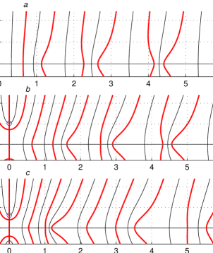
Figure 4: Zero level lines for real part (thick) and imaginary part (thin) (a) for Eq. (57) with $Q_{1}=Q_{2}=Q_{3}=1$; (b) for Eq. (60) with $Q_{1}=Q_{2}=Q_{3}=1$; (c) for Eq. (60), $Q_{1}=1$, $Q_{2}=0{.}2$, $Q_{3}=0{.}4$

In Fig. 4a the thick and thin lines are zero level lines correspondingly present real and imaginary part of the l.h.s. $f(\xi)=f(\xi_{1}+i\xi_{2})$ of Eq. (57) for given values $Q_{j}$. Roots of this equation are shown as cross points of a thick line with a thin line. If the values (53) $Q_{j}$ are given, one can determine values $\omega$, $\underline{\sigma}_{2}$, $v_{j}$, $m_{j}/\gamma$ from Eqs. (44), (51), (53). In particular, values $\omega$, $Q_{1}$, $Q_{3}$ are connected by the relation

$$\omega(Q_{1}+Q_{3})=(\omega^{2}-Q_{1}Q_{3})\tan\pi\omega,$$ (58)

resulting from the mentioned equations.

Analysis of roots of Eq. (57) for various values $Q_{j}$, $m_{j}$ and $v_{j}$ shows, that for all values of mentioned parameters all these frequencies are real numbers (cross points lie on the real axis), therefore amplitudes of such fluctuations do not grow with growing time $t$.

Note that any complex frequency $\xi=\xi_{1}+i\xi_{2}$ with positive imaginary part $\xi_{2}$ result in exponential growth of the corresponding amplitude of disturbances

$$\psi_{k}^{3}=B_{k}^{3}\exp(-i\xi_{1}\tau)\cdot\exp(\xi_{2}\tau)$$

In this case the considered state will be unstable stab ; Unst09 .

To study small disturbances in the $e_{1},\,e_{2}$ plane we consider projections (scalar products) of equations (52) onto 3 vectors $e_{0}$, $e(\tau)$, $\acute{e}(\tau)$. They form the system of 12 differential equations with deviating arguments with respect to 9 unknown functions $\psi_{j\pm}$, $\acute{\psi}_{j\pm}$, $\delta_{2}$, if functions $\psi_{j\pm}^{0}$ are excluded via the orthonormality condition, Eqs. (50):

$$\dot{\psi}_{j\pm}^{0}=\pm c_{1}(e,\dot{\psi}_{j\pm})-v_{1}(\acute{e},\dot{\psi}_{j\pm}),\qquad c_{1}=\cos\underline{\sigma}_{2}\omega.$$

Only 9 from these 12 equations are independent ones. When we search solutions of this system in the form of harmonics (56)

$$\psi_{j\pm}=B_{j\pm}e^{-i\xi\tau},\quad\acute{\psi}_{j\pm}=\acute{B}_{j\pm}e^{-i\xi\tau},\quad 2a_{0}\delta_{2}=\Delta_{2}e^{-i\xi\tau},$$ (59)

we obtain the homogeneous system of 9 algebraic equations with respect to 9 amplitudes $B_{j\pm}$, $\acute{B}_{j\pm}$, $\Delta_{2}$ (it is convenient to use the linear combinations of them $A_{j\pm}=-i\xi B_{j\pm}-\omega\acute{B}_{j\pm}$, $\acute{A}_{j\pm}=-i\xi\acute{B}_{j\pm}+\omega B_{j\pm}$):

$$\begin{array}[]{c}K_{1}^{+}A_{1+}+K_{1}^{-}A_{1-}=\acute{K}_{1}^{+}\acute{A}_{1+}+\acute{K}_{1}^{-}\acute{A}_{1-},\\ (1-i\xi Q_{1}^{\xi})\,A_{1+}+(1+i\xi Q_{1}^{\xi})\,A_{1-}=\omega Q_{1}^{\xi}(\acute{A}_{1-}-\acute{A}_{1+}),\rule{0.0pt}{11.99998pt}\\ (v_{1}\Gamma_{1}-\omega Q_{1}^{\xi})(A_{1-}-A_{1+})\rule{0.0pt}{11.99998pt}\\ =(1-i\xi Q_{1}^{\xi})\,\acute{A}_{1+}+(1+i\xi Q_{1}^{\xi})\,\acute{A}_{1-},\rule{0.0pt}{11.99998pt}\\ c_{1}(A_{1+}-A_{2+})-v_{1}(\acute{A}_{1+}-\acute{A}_{2+})=0,\rule{0.0pt}{11.99998pt}\\ c_{1}(A_{1-}-A_{2-})+v_{1}(\acute{A}_{1-}-\acute{A}_{2-})=0,\rule{0.0pt}{11.99998pt}\\ K_{1}^{+}E_{3}^{+}A_{2+}+K_{1}^{-}E_{3}^{-}A_{2-}=\acute{K}_{1}^{+}E_{3}^{+}\acute{A}_{2+}+\acute{K}_{1}^{-}E_{3}^{-}\acute{A}_{2-},\rule{0.0pt}{11.99998pt}\\ K_{2}^{+}E_{3}^{+}A_{2+}+K_{2}^{-}E_{3}^{-}A_{2-}=\acute{K}_{2}^{+}E_{3}^{+}\acute{A}_{2+}+\acute{K}_{2}^{-}E_{3}^{-}\acute{A}_{2-},\rule{0.0pt}{11.99998pt}\\ (c_{1}-2\omega v_{1}Q_{2}^{\xi})\,E_{2}^{+}A_{1+}+c_{1}E_{2}^{-}A_{1-}+v_{1}E_{2}^{-}\acute{A}_{1-}-i\xi\Delta_{2}\rule{0.0pt}{11.99998pt}\\ =E_{2}^{+}\big{[}(v_{1}+2\omega c_{1}Q_{2}^{\xi})\,\acute{A}_{1+}-2\omega Q_{2}^{\xi}(v_{1}A_{2+}+c_{1}\acute{A}_{2+})\big{]},\rule{0.0pt}{11.99998pt}\\ \acute{K}_{1}^{+}E_{2}^{+}A_{1+}+\acute{K}_{1}^{-}E_{2}^{-}A_{1-}+K_{1}^{+}E_{2}^{+}\acute{A}_{1+}+K_{1}^{-}E_{2}^{-}\acute{A}_{1-}\rule{0.0pt}{11.99998pt}\\ =-(\xi^{2}+\omega^{2})\,\Delta_{2}.\rule{0.0pt}{11.99998pt}\end{array}$$

Here $\;Q_{j}^{\xi}=Q_{j}/(\xi^{2}-\omega^{2})$, $E_{j}^{\pm}=\exp(\mp i\xi\underline{\sigma}_{j})$,

$$\begin{array}[]{c}K_{1}^{\pm}=c_{1}\omega\mp iv_{1}\xi,\qquad\acute{K}_{1}^{\pm}=\pm v_{1}\omega+ic_{1}\xi,\\ K_{2}^{\pm}=\omega Q_{3}^{\xi}\sin\pi\omega-(1\pm i\xi Q_{3}^{\xi})\cos\pi\omega,\\ \acute{K}_{2}^{\pm}=\mp\omega Q_{3}^{\xi}\cos\pi\omega-(\pm 1+i\xi Q_{3}^{\xi})\sin\pi\omega.\end{array}$$

Nontrivial solutions of this system exist if the condition similar to Eq. (57) takes place. It may be reduced to the following equation

$$\frac{\xi}{Q_{2}}\cdot\frac{\xi^{2}-\omega^{2}}{\xi^{2}+\omega^{2}}=\sum_{j=1,3}\frac{(q_{j}-\xi^{2})\,\tilde{c}_{j}-2Q_{j}\xi\tilde{s}_{j}}{(q_{j}-\xi^{2})\,\tilde{s}_{j}+2Q_{j}\xi\tilde{c}_{j}}.$$ (60)

Here $q_{j}=Q_{j}^{2}(1+v_{j}^{-2})$.

Fig. 4b, c demonstrates roots $\xi=\xi_{n}$ of Eq. (60), corresponding to frequencies of small oscillations of the rotating system $q$-$q$-$q$ in the rotational plane. Unlike Eq. (57), describing oscillations in $z$- or $e_{3}$-direction, equation (60) always has two imaginary roots $\xi=\pm i\xi_{2}^{*}$. The positive imaginary roots $\xi=i\xi_{2}^{*}$, $\xi_{2}^{*}>0$ are marked with a circle in Fig. 4b, c.

Other roots of Eq. (60) are real ones. In Figs. 4b and 4a values $Q_{j}$, $m_{j}$ are the same, the mass relation here is $m_{1}:m_{2}:m_{3}\simeq 1:1.85:1$; for the case in Fig. 4c it is $m_{1}:m_{2}:m_{3}\simeq 1:10.5:4.2$.

The positive imaginary root $\xi=i\xi_{2}^{*}$ of Eq. (60) may be found after substituting $\xi=i\xi_{2}$:

$$\frac{\xi_{2}}{Q_{2}}\cdot\frac{\xi_{2}^{2}+\omega^{2}}{\omega^{2}-\xi_{2}^{2}}=\sum_{j=1,3}\frac{q_{j}+\xi_{2}^{2}+2Q_{j}\xi_{2}\tanh\check{\sigma}_{j}\xi_{2}}{(q_{j}+\xi_{2}^{2})\,\tanh\check{\sigma}_{j}\xi_{2}+2Q_{j}\xi_{2}}.$$

Here $\check{\sigma}_{1}=\underline{\sigma}_{2}$, $\check{\sigma}_{3}=\pi-\underline{\sigma}_{2}$. Evidently, the required value $\xi^{*}$ exists in the interval $(0,\omega)$. An arbitrary disturbed motion of the $q$-$q$-$q$ configuration contains exponentially growing modes in its spectrum, in particular,

$$\psi_{j\pm}=B_{j\pm}\exp(\xi_{2}^{*}\tau).$$ (61)

So the rotational motion (43) is unstable with respect to small disturbances. Evolution of this instability was numerically analysed in Ref. stab .

V Rotational states for closed string

For the case of closed string rotational states (planar uniform rotations of the string with massive points) were described and classified in Refs. PRTr ; glY08 . These states are divided into 3 classes glY08 : “hypocycloidal states” (in this case segments of rotating string, connecting massive points, are segments of a hypocycloid), “linear states” and “central states”, describing rotating folded closed string with rectilinear string segments. For linear states all masses $m_{j}$ move at nonzero velocities $v_{j}$, but in the case of central states a massive point (or some of them) is placed at the rotational center.

In Ref. Unst09 we solved the stability problem for the central rotational states with $n=3$ massive points where the mass $m_{3}$ is at the center and other masses $m_{1}$ and $m_{2}$ rotates at the ends of rectilinear segments. These states look like the states (43) of the linear model $q$-$q$-$q$, but have the additional string segment (the string is closed) and another numeration of massive points.

The mentioned central states with $n=3$ have the form

$$\underline{X}^{\mu}=e_{0}^{\mu}a_{0}\tau+u(\sigma)\cdot e^{\mu}(\tau),$$ (62)

where $u(\sigma)=A_{j}\cos\omega\sigma+B_{j}\sin\omega\sigma$, $\sigma\in[\sigma_{j-1},\sigma_{j}]$ is continuous function, but its derivatives has discontinuities at $\sigma=\sigma_{j}\equiv\underline{\sigma}_{j}={}$const (positions of masses $m_{j}$). They are described by following parameters, determined by Eqs. (2), (3), (7), (8): $A_{1}=0$, $\underline{\sigma}_{2}-\underline{\sigma}_{1}=\pi$, $A_{2}=2\breve{S}_{1}\breve{C}_{1}B_{1}$, $B_{2}=(\breve{S}_{1}^{2}-\breve{C}_{1}^{2})B_{1}$, $A_{3}=-\breve{S}B_{1}$, $B_{3}=\breve{C}B_{1}$; $v_{1}=\breve{S}_{1}$, $v_{2}=\sin(2\pi-\underline{\sigma}_{2})\omega$. Here

$$\breve{C}_{j}=\cos\omega\underline{\sigma}_{j},\quad\breve{S}_{j}=\sin\omega\underline{\sigma}_{j},\quad\breve{C}\equiv\breve{C}_{3},\quad\breve{S}\equiv\breve{S}_{3},$$

the closure condition (2) takes the form $\tau^{*}=\tau$ the values (53) $\gamma m_{j}^{-1}\sqrt{\dot{X}^{2}(\tau,\underline{\sigma}_{j})}=Q_{j}$ are constants.

For these rotational states the string rotates at the angular velocity $\Omega=\omega/a_{0}$, the value $a_{0}$ connected with speeds $v_{j}$ of massive points by the following equations, resulting from Eqs. (53):

$$a_{0}=\frac{m_{1}Q_{1}}{\gamma\sqrt{1-v_{1}^{2}}}=\dots=\frac{m_{n}Q_{n}}{\gamma\sqrt{1-v_{n}^{2}}}.$$ (63)

The central rotational states (62) were tested for stability in Ref. Unst09 . In this paper the approach suggested in Sect. IV for states (43) was used. Here we omit details of this investigation and present its results: the central states (62) appeared to be unstable (small disturbances grow) if the central mass is less than the critical value

$$0<m_{3}<m_{3cr},$$ (64)

$$m_{3cr}=2\pi\gamma a_{0}+\frac{m_{1}}{\sqrt{1-v_{1}^{2}}}+\frac{m_{2}}{\sqrt{1-v_{2}^{2}}}\equiv E-m_{3}.$$

Here is energy of the state (62). We may conclude, the central rotational state is unstable if the central mass $m_{3}$ is nonzero and less than energy of the string with other massive points. Note that in the case of the linear string model in Sect. IV there were no such a threshold effect.

If $m_{3}$ satisfies the condition (64), the spectrum of small disturbances of the central rotational states (62) has complex frequencies. This results in exponential growth of small disturbances in accordance with the expression (61).

In the case $m_{3}=0$ there is no massive point at the center, and the corresponding linear rotational state with $n=2$ is stable. Stability also takes place for the case $m_{3}\to\infty$.

VI Instability of rotational states and hadron’s width

Rotational states (17) of the string model Y and (43) of the linear string model were applied for describing orbitally excited baryons 4B ; InSh . The similar states (62) of the closed string describe the Pomeron trajectory glY08 , corresponding to possible glueball states.

For rotational states (17), (43) and (62) energy $E$ or mass $M$ and angular momentum $J$ are determined by the following expressions 4B ; InSh ; glY08 :

$$M=E = q\pi\gamma a_{0}+\sum_{j=1}^{n}\frac{m_{j}}{\sqrt{1-v_{j}^{2}}}+\Delta E_{SL},$$ (65)

$$J=L+S = \frac{a_{0}}{2\omega}\bigg{(}q\pi\gamma a_{0}+\sum_{j=1}^{n}\frac{m_{j}v_{j}^{2}}{\sqrt{1-v_{j}^{2}}}\bigg{)}+\sum_{j=1}^{n}s_{j}.\qquad\$$ (66)

Here $q=1$ for the linear model, $q=2$ for the closed string, $q=3$ for the Y model, $s_{j}$ are spin projections of massive points (quarks or valent gluons), $\Delta E_{SL}$ is the spin-orbit contribution to the energy in the form 4B

$$\Delta E_{SL}=\sum_{j=1}^{n}\big{[}1-(1-v_{j}^{2})^{1/2}\big{]}(\textbf{$\Omega$}\cdot\textbf{s}_{j}).$$

If the string tension $\gamma$, values $m_{j}$ and $s_{j}$ are fixed, we obtain the one-parameter set of rotational states (17), (43) or (62). Values $J$ and $E^{2}$ for these states form the quasilinear Regge trajectory with asymptotic behavior $J\simeq\alpha_{0}+\alpha^{\prime}E^{2},$ for large $E$ and $J$ 4B ; glY08 with the slope $\alpha^{\prime}=1/(2\pi\gamma)$ for the linear quark-diquark models, $\alpha^{\prime}=1/(3\pi\gamma)$ for states (17) of the Y model and $\alpha^{\prime}=1/(3\pi\gamma)$ for states (62) of the closed string.

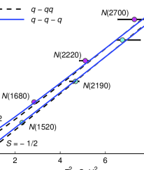
Figure 5: Regge trajectories for rotational states (43) of the linear baryon model (solid lines) and the quark-diquark model (dashed lines)

Fig. 5 presents the typical picture of Regge trajectories for $N$ baryons with $J^{P}=1/2^{+},3/2^{-},5/2^{+},\dots$ generated by the linear baryon model (solid lines) in comparison with the quark-diquark model (dashed lines).

Here the model parameters are taken from Ref. 4B :

$$\gamma=0{.}175\mbox{ GeV}^{2},\quad m_{q}=130\mbox{ MeV},\quad m_{qq}=2m_{q}$$ (67)

This tension corresponds to the slope $\alpha^{\prime}\simeq 0{.}9$ GeV^-2, effective masses of light quarks are less than constituent masses 4B ; InSh .

One can see that predictions of the linear baryon model $q$-$q$-$q$ and the quark-diquark model $q$-$qq$ are rather close under conditions (67). The similar picture takes place for baryons $\Delta$ and strange baryons 4B ; InSh .

We have shown in Sect. IV that the rotational states (43) of the linear string model are unstable for all energies on the classic level. But this does not mean disappearance or terminating corresponding Regge trajectories in Fig. 5. The straight consequence of this instability is the contribution to width of a hadron state.

String models describe only excited hadron states with large orbital momenta $L$. These states are unstable with respect to strong decays and have rather large width $\Gamma$. In string interpretation this width is connected with probability of string breaking; this probability is proportional to the string length $\ell$ Kodecay ; GuptaR . The value $\ell$ is proportional to the string contribution $E_{str}$ to energy $E$ of a hadron state. For rotational states (43) and (62) this contribution to the expression (65) is $E_{str}=q\pi\gamma a_{0}$.

Therefore, the component of width $\Gamma_{br}$, connected with string breaking, is proportional to $E_{str}$ with the factor $0{.}1$ resulting from particle data Kodecay ; GuptaR ; PDG :

$$\Gamma_{br}\simeq 0{.}1\cdot E_{str}=0{.}1\cdot q\pi\gamma a_{0}.$$ (68)

If a state of a string system is unstable with respect to small disturbances on the classical level, we are to take this instability into account in the form of additional summand in width $\Gamma$ of this hadron state:

$$\Gamma=\Gamma_{br}+\Gamma_{inst}.$$ (69)

The contribution $\Gamma_{inst}$ due to the mentioned instability is determined by the increment $\xi_{2}=\xi_{2}^{*}$ of exponential growth (61)

$$|\psi|\sim\exp(\xi_{2}^{*}\tau)=\exp(\xi_{2}^{*}a_{0}^{-1}t)$$

and relation $t=a_{0}\tau$ for rotational states (43) and (62). So for these states

$$\Gamma_{inst}\simeq\frac{\xi_{2}^{*}}{a_{0}}.$$ (70)

The values $\xi_{2}^{*}$, $a_{0}$ and both summands (68) and (70) of the width (69) depend on energy $E$ of the hadron state. This dependence for values $\xi_{2}^{*}$, $\Gamma_{inst}$, $\Gamma_{br}$, and $\Gamma$ is calculated for rotational states (43) of the model $q$-$q$-$q$, corresponding to parameters (67) for the $N$ baryons in Fig. 6. These graphs are presented in Fig. 6a in comparison with experimental widths of $N$ and $\Delta$ baryons PDG lying on main Regge trajectories. These widths are shown as the bar graph with dark bars for $N$ baryons mentioned in Fig. 5 and light bars for baryons $\Delta(1232)$, $\Delta(1930)$, $\Delta(2420)$, $\Delta(2950)$.

Note that the dimensionless value $\xi_{2}^{*}=\xi_{2}^{*}(E)$ tends to zero at $E\to E_{min}=\sum m_{j}$, but $a_{0}$ tends to zero more rapidly, so width $\Gamma_{inst}$ (70) tends to infinity.

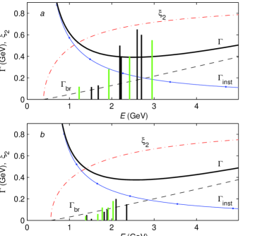
Figure 6: Width $\Gamma=\Gamma(E)$ (69) (solid line), its summands $\Gamma_{br}$ (68) (dashed line) and $\Gamma_{inst}$ (70) (line with dots) for states (43) of the model $q$-$q$-$q$ (a) with parameters (67); (b) with $m_{2}=300$ MeV

In Fig. 6b the similar graphs for strange baryons with $m_{2}\equiv m_{s}=300$ MeV, $m_{1}=m_{3}=130$ MeV are presented. Here dark bars show width of baryons $\Lambda(1405)$, $\Lambda(1520)$, $\Lambda(1820),\dots$, light bars correspond to $\Sigma(1385)$, $\Sigma(1670)$, $\Sigma(1775)$, $\Sigma(2030)$.

In the mass range 1 – 2.8 GeV the contribution $\Gamma_{inst}$ (70) due to instability of the linear model exceeds $\Gamma_{br}$ and tend to infinity at $E\to E_{min}$. This behavior contradicts experimental data of baryon’s width in the mentioned mass range: $\Gamma$ tends to zero if $E\to E_{min}$. So one may conclude that the linear baryon model $q$-$q$-$q$ is not adequate for describing orbitally excited baryon stated as the consequence of rotational instability of this model.

If we use this approach to the string baryon model Y, we conclude that instability of rotational states (17) does not change effective hadron’s width $\Gamma$, because linear growth of small disturbances corresponds to zero contribution $\Gamma_{inst}=0$ in the increment (factor in the exponent of expression (61)).

Hence for the Y configuration width $\Gamma$ equals $\Gamma_{br}$, the figure similar to Fig. 6 will have only dashed line for $\Gamma=\Gamma(E)$ in this case.

We mentioned above that unstable central rotational states (62) of the closed string, considered in Sect. V, may be applied for describing the Pomeron trajectory

$$J\simeq 1{.}08+0{.}25E^{2}$$ (71)

corresponding to possible glueball states glY08 ; MeyerT .

Estimations of gluon masses on the base of gluon propagator in lattice calculations BonnBLW ; SilvaO yield values $m_{j}$ from 700 to 1000 MeV. We suppose that gluon masses $m_{j}=750$ MeV and string tension $\gamma=0{.}175\mbox{ GeV}^{2}$ corresponds to the value (67). These parameters result in Regge trajectories $J=J(E^{2})$ for states (62) close to the Pomeron trajectory (71) glY08 .

In Fig. 7a the total width $\Gamma=\Gamma(E)$ (69) with its summands $\Gamma_{br}$ and $\Gamma_{inst}$ calculated in Ref. Unst09 is presented for central rotational states (62). They are unstable for all energies $E$, if masses $m_{j}$ are equal. The corresponding width $\Gamma_{inst}(E)$ tends to infinity in the limit $E\to E_{min}=\sum m_{j}$.

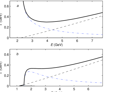
Figure 7: Width $\Gamma(E)$ (69) (solid line) as the sum of $\Gamma_{br}$ (68) (dashed line) and $\Gamma_{inst}$ (70) (dash-dotted line) for central states (62) of the closed string (a) with parameters $m_{j}=750$ MeV; (b) with $m_{1}=m_{2}=200$ MeV, $m_{3}=750$ MeV

Behavior of width $\Gamma(E)$ (69) for central rotational states of the system with $m_{3}>m_{1}+m_{2}$ is presented in Fig. 7b. In this case the threshold effect (64) exists, so the “instability” width $\Gamma_{inst}(E)$ equals zero for energies $E<E_{cr}=2m_{3}$ (here it is 1.5 GeV). For $E>E_{cr}$ $\Gamma_{inst}(E)$ exceeds $\Gamma_{br}(E)$ in the certain interval, but if $E$ grows, $\Gamma_{inst}(E)$ tends to zero and $\Gamma_{br}(E)$ increases.

VII Conclusion

The stability problem was solved for classic rotational states (17) of the Y string baryon model and (43) of the linear string baryon model in comparison with states (62) for the closed string with massive points. It was shown for all models that the mentioned rotations are unstable, but this instability has different specific features. For the linear model spectra of small disturbances for states (43) contain complex frequencies for any nonzero values of masses $m_{j}$. They are roots of Eqs. (60). These frequencies $\xi=\xi_{1}+i\xi_{2}$ correspond to exponentially growing modes of disturbances $\psi\sim\exp(\xi_{2}\tau)$ and, consequently, to instability of the mentioned rotational states.

The similar behavior takes place for the closed string, but in this case we have the threshold effect, the central rotational states (62) unstable, if the central mass is nonzero and less than the critical value $m_{cr}$ (64). This critical value equals energy of the string without the central mass.

Rotational instability of the string Y configuration has another nature. There is no complex frequencies $\xi=\xi_{1}+i\xi_{2}$ in the spectrum (60) of small disturbances for states (17), but this spectrum contains double roots $\xi=\pm\omega$ resulting in existence of disturbances (oscillatory modes) with linearly growing amplitudes.

Instability of classic rotations results in some manifestations in properties of hadron states, described by the considered string model. In particular, such a model predicts additional width $\Gamma_{inst}$ (70) of excited hadrons. Analysis in Sect. VI shows, that the contribution $\Gamma_{inst}$ in total width $\Gamma$ (69), predicted by the linear string baryon model $q$-$q$-$q$ in the mass range 1 – 3 GeV is too large in comparison with experimental data for $N$, $\Delta$ and strange baryons. These predictions very weakly depend on quark masses $m_{j}$ as model parameters. So we conclude, that the linear string model $q$-$q$-$q$ is unacceptable for describing these baryon states and we should refuse this model in favor of the quark-diquark and Y models.

Nevertheless, we can not exclude the $q$-$q$-$q$ configuration as possible structure of some baryons with anomalously large width or a variant of mixing with other configurations. To make a definite conclusion for the closed string, considered in Sect. V, we are to have more reliable experimental data for glueballs and exotic hadrons.

For the Y string baryon model linear (not exponential) growth of small disturbances corresponds to zero contribution $\Gamma_{inst}=0$ in the increment of instability in the exponent of expression (61). So instability of rotational states (17) does not give an additional contribution in width $\Gamma$ of baryons, describing with the Y string model. This rotational instability of states (17) is not an argument against application of the Y configuration. But this model has another drawback, it predicts the slope $\alpha^{\prime}=(3\pi\gamma)^{-1}$ for Regge trajectories different from the value $\alpha^{\prime}=(2\pi\gamma)^{-1}$ for the string meson model Ko ; 4B .

References

• (1) Y. Nambu, Phys. Rev. D 10, 4262 (1974).
• (2) A. Chodos and C. B. Thorn, Nucl. Phys. B 72, 509 (1974).
• (3) X. Artru, Nucl. Phys. B 85, 442 (1975).
• (4) G. S. Sharov, Phys. Atom. Nucl. 62, 1705 (1999).
• (5) I. Yu. Kobzarev, B. V. Martemyanov, and M. G. Shchepkin, Sov. Phys. Usp. 35, 257 (1992).
• (6) V. P. Petrov and G. S. Sharov, Mathem. Modelirovanie, 11, 39 (1999), [arXiv:hep-ph/9812527].
• (7) M. S. Plyushchay, G. P. Pronko, and A. V. Razumov. Theor. Math. Phys. 63, 389 (1985).
• (8) G. S. Sharov, Phys. Rev. D 58, 114009 (1998).
• (9) A. Inopin, G. S. Sharov, Phys. Rev. D63, 054023 (2001).
• (10) L. D. Soloviev, Phys. Rev. D 61, 015009 (1999).
• (11) G. S. Sharov. Phys. Rev. D 62, 094015 (2000).
• (12) G. S. Sharov, Phys. Atom. Nucl. 65, 906 (2002).
• (13) L. D. Soloviev, Theor. Math. Phys. 126, 203 (2001).
• (14) F. J. Llanes-Estrada et al., Nucl. Phys. A 710, 45 (2002).
• (15) L. A. Pando Zayas, J. Sonnenschein, and D. Vaman, Nucl. Phys. B 682, 3 (2004).
• (16) G. S. Sharov, Phys. Atom. Nucl. 71, 574 (2008).
• (17) G. S. Sharov, Phys. Rev. D 79, 114025 (2009).
• (18) G. S. Bali, Phys. Rev. D 62, 114503 (2000).
• (19) H. B. Meyer and M. Teper, Phys. Lett. B 605, 344 (2005).
• (20) I. Yu. Kobzarev, B. V. Martemyanov, and M. G. Shchepkin, Sov. J. Nucl. Phys. 48, 344 (1988).
• (21) K. S. Gupta and C. Rosenzweig. Phys. Rev. D 50, 3368 (1994).
• (22) G. S. Sharov, Theor. Math. Phys. 140, 242 (2004).
• (23) A. E. Milovidov and G. S. Sharov, Theor. Math. Phys. 142, 61 (2005).
• (24) C. Amsler et al., Particle Data Group. PL B667, 1 (2008).
• (25) F. D. R. Bonnet, P. O. Bowman, D. B. Leinweber and A. G. Williams, Phys. Rev. D 62, 051501(R) (2000).
• (26) P. J. Silva and O. Oliveira, Nucl. Phys. B 690, 177 (2004).