Bistable Stochastic Processes in the $q$-Exponential Family

Abstract

Stochastic bistable systems whose stationary distributions belong to the $q$-exponential family are investigated using two approaches: (i) the Langevin model subjected to additive and quadratic multiplicative noise, and (ii) the superstatistical model. Previously, the bistable Langevin model has been analyzed under linear multiplicative noise, whereas this paper reports on quadratic multiplicative noise, which is more physically meaningful. The stationary distribution of the Langevin model under quadratic multiplicative noise, which agrees with that derived by the maximum Tsallis entropy method, is found to be qualitatively different from its counterpart under linear multiplicative noise. We also show that the stationary distribution of the superstatistical model is the same as that of the Langevin model, whereas their transient properties, described in terms of mean first passage times (MFPTs), are qualitatively different.

I Introduction

The exponential family given by

$$\rho(x;\beta):=\exp\left[-\theta(\beta)-\beta H(x)\right],$$ (1)

is of great interest in physics, because of its relevance to many physical phenomena ($\beta$ is inverse temperature, $\theta(\beta)$ is a normalization term and $H(x)$ is the Hamiltonian). The exponential family includes the Gibbs measure, the canonical ensemble and the Gaussian distribution as special cases. The exponential family is important, since it appears as the limiting distribution of the central limit theorem, as distributions which maximize the Boltzmann-Gibbs-Shannon (BGS) entropy and also as stationary distributions of stochastic processes.

In recent years, many investigations Tsallis:1988:Generalization ; Tsallis:2004:NextEntBook ; Suyari:2005:LawOfError ; Umarov:2006:q-Fourier ; Rodriguez:2008:CorBinary ; Tsallis:2009:NonextensiveBook ; Hasegawa:2009:MqLE have been made of physical phenomena which belong to the $q$-exponential family (such as the nonextensive canonical ensemble and the $q$-Gaussian distribution) Naudts:2008:GenExpFam ; Naudts:2009:qExpFamily :

$$\rho_{q}(x;\beta):=\exp_{q}\left[-\theta(\beta)-\beta H(x)\right],$$ (2)

where $q$ is an entropic index and $\exp_{q}(x)$ is the $q$-exponential function [see Eq. (7)]. The $q$-exponential family is a one parameter generalization of the conventional exponential family, and reduces to the exponential family as $q\rightarrow 1$. The $q$-exponential family can account for systems where physical quantities such as energy and entropy are not proportional to system size (nonextensive). As the conventional exponential family, the $q$-exponential family also plays an important role in stochastic processes. For example, particles under a quadratic potential driven by additive and linear multiplicative noise satisfy a $q$-Gaussian as their stationary distributions Anteneodo:2003:MultBrownian .

In stochastic processes, bistable potentials are highly important in many fields including physics, electronics, biology and chemistry. It has been applied to chemical reactions, optical bistability, electric circuits, gene expression mechanisms and all the rest. Bistable stochastic processes can model switching dynamics of two-states systems under fluctuant environments. For bistable systems, multiplicative noise plays an essential role, and phenomena such as resonant activation Doering:1992:ResonantActivation ; Marchi:1996:ResoAct and noise-enhanced stability Mantegna:1996:NES ; Spagnolo:2008:NES_review emerge only in the presence of multiplicative noise. In these studies, linear multiplicative noise has been exclusively assumed, since it is straightforward to analytically obtain its stationary distribution. In this paper, on the other hand, we study quadratic multiplicative noise for a quartic bistable system. Considering a physical meaning of multiplicative noise, we show that quadratic multiplicative noise for the quartic potential is a straightforward extension of linear multiplicative noise for the quadratic potential. The quadratic multiplicative noise inherits an important property, namely that the noise intensity vanishes at stable sites, in the same way as intensity of linear multiplicative noise also vanishes at a stable site of the quadratic potential. In this paper, we investigate the stationary and transient properties of bistable quartic systems subjected to quadratic multiplicative noise. We show that the resulting stationary distribution belongs to the $q$-exponential family [Eq. (2)], which agrees with a maximizer of the Tsallis entropy under constraints. Since much attention has been paid to the $q$-exponential aspect of physical phenomena in recent years, it is important to investigate bistable systems which belong to the $q$-exponential family. We first study stationary distributions of the quadratic multiplicative case, comparing them with those of the linear multiplicative case for the quartic bistable potential. From these analyses, we show that the effects of multiplicative noise are different in each system.

One of the alternative approaches yielding the $q$-exponential is superstatistics Wilk:2000:NEXTParam ; Beck:2003:Superstatistics ; Beck:2005:Superstatistics . Superstatistics can model or describe quasi-equilibrium systems, where environments fluctuate spatially and/or temporally. In recent years, Ref. Rodriguez:2007:SS_Brownian derived the superstatistical Brownian motion from the viewpoint of mesoscopic nonequilibrium thermodynamics Mazur:1999:MNET . The concept of superstatistics has been extended to the path-integral Jizba:2008:SuposPD , and it was shown that the path-integral superstatistics include a financial model with stochastic volatility Heston:1993:Volatility . These studies show that superstatistics is highly important for modeling and understanding of many real world phenomena. Regarding a relation to the $q$-exponential distributions, Ref. Beck:2006:SS_Brownian showed that Brownian particles moving in fluctuant environments satisfy the $q$-Gaussian as their stationary distributions. Therefore, we apply the superstatistical concept to the quartic bistable potential, and show that the stationary distributions belong to the $q$-exponential family in the small noise limit.

In order to investigate transient properties of bistable stochastic processes in the $q$-exponential family, we calculate the mean first passage time (MFPT). We obtain the approximate analytic expression of MFPTs for the two cases of the Langevin model with quadratic multiplicative noise and superstatistics. We find that the $q$-dependence of MFPTs in the two cases is completely different, although their stationary distributions are the same. We also see a formal nonextensive generalization in two MFPTs: $\exp(x)$ is replaced by $\exp_{2-q}(x)$ in the quadratic multiplicative case and by $\exp_{q}(x)$ in the superstatistical case.

This paper is organized as follows: In Sec. II, we first derive stationary distributions by the Langevin equation with quadratic multiplicative noise model and superstatistical approach. We next proceed to the calculation of MFPTs in Sec. III. In Sec. IV, we discuss the validity of our quadratic multiplicative noise from the viewpoint of an open quantum system. Effects of correlation between additive and multiplicative noise are also discussed. We conclude this paper in Sec. V.

II Stationary Distribution

II.1 Maximum Tsallis Entropy Principle

In nonextensive statistics, many important distributions can be derived from the maximum Tsallis entropy principle. The Tsallis entropy is given by

$$S_{q}:=\frac{{\displaystyle 1-\int dx\,P(x)^{q}}}{q-1},$$ (3)

where $q$ is an entropic index and Eq. (3) reduces to the BGS entropy in the limit as $q\rightarrow 1$. Adopting the optimal Lagrange multiplier (OLM) maximum entropy method Martinez:2000:OLMMEM with the constraints,

$$\int dx\,P(x) = 1,$$ (4)

$$\int dx\,\mathscr{P}_{q}(x)U(x) = U_{q},$$ (5)

we obtain the distribution given by

$$P(x)=\exp_{q}\left[-\ln_{2-q}Z-\beta\left(U(x)-U_{q}\right)\right].$$ (6)

Here $U(x)$ denotes a potential, $\mathscr{P}_{q}(x)$ is the escort distribution defined by $\mathscr{P}_{q}(x):=P(x)^{q}/\int dx\,P(x)^{q}$, $Z$ is a normalization constant and $\exp_{q}(x)$ denotes the $q$-exponential function defined by

$$\exp_{q}(x):=[1+(1-q)x]_{+}^{1/(1-q)},$$ (7)

where $[x]_{+}:=\max(x,0)$. Its inverse function, the $q$-logarithm, is defined by

$$\ln_{q}(x):=\frac{x^{1-q}-1}{1-q}\,\,\,(\mathrm{for}\,\,\,x>0).$$ (8)

With the use of these generalized functions, important nonextensive distributions can be expressed in a similar form to that of conventional ones.

II.2 The Langevin Model Subjected to Quadratic Multiplicative Noise

Figure 1: (Color online) (a) A quadratic potential with linear multiplicative noise and (b) a quartic potential with quadratic multiplicative noise. Solid and dashed lines represent the potentials and multiplicative terms, respectively.

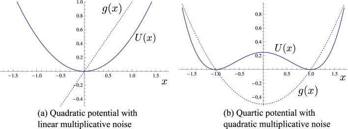
We here consider the following Langevin equation:

$$\frac{dx}{dt}=f(x)+g(x)\xi(t)+\eta(t),$$ (9)

where $f(x):=-U^{\prime}(x)$ and $g(x)$ is a multiplicative term. $\xi(t)$ and $\eta(t)$ are white Gaussian noise with correlations:

$$\left\langle\xi(t)\xi(s)\right\rangle=2M\delta(t-s),$$ (10)

$$\left\langle\eta(t)\eta(s)\right\rangle=2A\delta(t-s),$$ (11)

$$\left\langle\eta(t)\xi(s)\right\rangle=\left\langle\xi(t)\eta(s)\right\rangle=0,$$ (12)

where $A$ and $M$ represent intensity of additive and multiplicative noise, respectively.

The Fokker-Planck equation (in Stratonovich’s sense) of Eq. (9) is given by

$$\frac{\partial}{\partial t}P(x,t)=-\frac{\partial}{\partial x}F(x)P(x,t)+\frac{\partial^{2}}{\partial x^{2}}G(x)P(x,t),$$ (13)

where

$$F(x)=f(x)+Mg(x)g^{\prime}(x),$$ (14)

$$G(x)=A+Mg(x)^{2}.$$ (15)

If $g(x)$ and $f(x)$ satisfy

$$f(x)=-\kappa g(x)g^{\prime}(x),$$ (16)

or identically

$$U(x)-U_{0}=\frac{\kappa}{2}g(x)^{2},$$ (17)

the stationary distributions are the $q$-exponential distributions as will be shown shortly [Eq. (24)] ($\kappa>0$ is a proportional constant and $U_{0}$ is the minimum of the potential) Anteneodo:2003:MultBrownian . We study a simple quartic bistable potential given by

$$U(x)-U_{0}=\frac{1}{4}\left(x^{2}-1\right)^{2}.$$ (18)

As a consequence, we consider the following multiplicative term:

$$g(x)=\frac{1}{\sqrt{2\kappa}}(x^{2}-1).$$ (19)

We next consider a physical meaning of the quadratic multiplicative noise of Eq. (19). For the case of stochastic processes with a quadratic potential and linear multiplicative noise (Fig. 1 (a)), the stationary distributions are $q$-Gaussian. In this case, the nonextensivity is derived from the linear multiplicative noise [$g(x)=x$]. This linear multiplicative noise is natural in some cases, because the intensity of the multiplicative noise vanishes at stable positions and the intensity of the noise is greater when a particle is at more unstable states. Extending this property to the quartic bistable potential [Eq. (18)], it may be natural to allow the intensity of multiplicative noise at the two stable sites to vanish. Because the multiplicative term defined by Eq. (19) inherits this property (Fig. 1 (b)), it is considered that Eq. (19) is a straightforward extension of the linear multiplicative noise for quadratic potentials. In Sec. IV.1, a quantum interpretation for the multiplicative noise is discussed.

We next calculate the stationary distribution. By calculating the stationary solution of the Fokker-Planck equation of Eq. (13), we obtain the following distribution:

$$P_{st}(x)\propto\exp\left(-V(x)\right),$$ (20)

with an effective potential $V(x)$:

$$V(x) := -\int^{x}du\frac{F(u)}{G(u)}+\ln G(x),$$ (21)

$$= -\int^{x}du\frac{(M-\kappa)g(u)g^{\prime}(u)}{A+Mg(u)^{2}}+\ln\left(A+Mg(x)^{2}\right),$$ (22)

$$= \frac{\kappa+M}{2M}\ln\left(A+\frac{2M}{\kappa}\left(U(x)-U_{0}\right)\right).$$ (23)

Equations (20) and (23) are the $q$-exponential family [Eq. (2)], since they can be rewritten as

$$P_{st}(x)=\exp_{\widehat{q}}\left[-\ln_{2-\widehat{q}}\widehat{Z}-\widehat{\beta}\left(U(x)-U_{0}\right)\right],$$ (24)

where

$$\widehat{\beta}=\widehat{\beta}_{0}\cdot\widehat{Z}^{\widehat{q}-1},\,\,\,\,\widehat{\beta}_{0}=\frac{\kappa+M}{\kappa A},\,\,\,\widehat{q}=\frac{\kappa+3M}{\kappa+M},$$ (25)

$\widehat{Z}$ being a normalization constant.

We plotted Eq. (20) with Eq. (23) in Fig. 2 with $\kappa=2$ ($\widehat{Z}$ is evaluated using numerical integration). For comparison, we also show in Fig. 3 the stationary distributions for the linear multiplicative case [$g(x)=x$] with the quadratic potential given by Eq. (18), for which an effective potential $V(x)$ is given by

$$V(x) = -\int^{x}du\frac{(M+1)u-u^{3}}{A+Mu^{2}}+\ln\left(A+Mx^{2}\right),$$

$$= \frac{x^{2}}{2M}+\frac{1}{2}\left(1-\frac{1}{M}-\frac{A}{M^{2}}\right)\ln\left(A+Mx^{2}\right)\,\,\,(\mathrm{for}\,\,g(x)=x).$$

For the case of quadratic multiplicative noise (Fig. 2), the stationary distributions always exhibit bi-modality. We can see that the effect of $M$ of quadratic multiplicative noise is different from that of linear one as shown in Figs. 2 and 3. For the case of linear multiplicative noise, larger $M$ makes the probability density around $x=0$ higher. With $M\geq 1$, the stationary distribution for the linear multiplicative noise case is uni-modal (Fig. 3). For $M<1$, the stationary distribution has two modals at $x=\pm\sqrt{1-M}$. This indicates that stable positions for the effective potential are not at $x=\pm 1$. On the other hand, the intensity of $M$ behaves differently for quadratic multiplicative noise. In Fig. 2 (a), the density at stable sites ($-1$ and $1$) is smaller for large $M$. Conversely, the density of stable sites ($1$ and $-1$) is higher for larger $M$ in Fig. 2 (c). From this result, we can see that effects of quadratic multiplicative noise depend on the intensity of the additive noise.

Figure 2: (Color online) Stationary distributions for quadratic multiplicative noise with each parameter setting ($\kappa=2$).

Figure 3: (Color online) Stationary distributions for linear multiplicative noise with each parameter setting.

II.3 Superstatistical Model

We next describe bistable systems of the $q$-exponential family from the viewpoint of superstatistics. Superstatistics Wilk:2000:NEXTParam ; Beck:2003:Superstatistics ; Beck:2005:Superstatistics has been developed to describe quasi-equilibrium systems, where parameters describing environments fluctuate spatially and/or temporally, because many physical systems are inhomogeneous. Let $h(\beta;\beta_{0})$ be a PDF of $\beta$, where $\beta_{0}$ is a hyper-parameter of the distribution. In general cases, superstatistics is given by calculating the expectation of the Gibbs measure $\rho(\varepsilon_{i}|\beta)$ in terms of $h(\beta;\beta_{0})$:

$$P(\varepsilon_{i};\beta_{0})=\int_{0}^{\infty}d\beta\,\,\rho(\varepsilon_{i}|\beta)h(\beta;\beta_{0}).$$ (26)

Equation (26) defines the so-called “Type-B” superstatistics. By taking $h(\beta;\beta_{0})$ as the prior distribution, superstatistics can be considered as a Bayesian framework Sattin:2006:BayesToSuper ($P(\varepsilon_{i};\beta_{0})$ corresponds to a posterior). For $h(\beta;\beta_{0})=\delta(\beta-\beta_{0})$, Eq. (26) reduces to the Gibbs measure.

Superstatistics can also be applied to the description of Brownian particles, where the particles are in inhomogeneous environments. Ref. Beck:2006:SS_Brownian has reported that superstatistical Brownian particles follow $q$-Gaussian distributions.

Superstatistics assumes Brownian particles in inhomogeneous environments. The superstatistical Brownian model assumes the following Langevin equation, driven by additive Gaussian white noise:

$$\frac{dx}{dt}=f(x)+\zeta(t),$$ (27)

$$\left\langle\zeta(t)\zeta(s)\right\rangle=2\alpha\delta(t-s),$$ (28)

where $f(x):=-U^{\prime}(x)$ and $\alpha$ is noise intensity. We first calculate the stationary distribution in a given sub-system driven by additive noise, which is represented by

$$\rho(x)=\frac{1}{Z(\alpha)}\exp\left[-\frac{U(x)-U_{0}}{\alpha}\right],$$ (29)

with

$$Z(\alpha) = \int_{-\infty}^{\infty}dx\,\exp\left[-\frac{U(x)-U_{0}}{\alpha}\right]$$

$$= \frac{\pi}{2}\exp\left(-\frac{1}{8\alpha}\right)\left[I_{-\frac{1}{4}}\left(\frac{1}{8\alpha}\right)+I_{\frac{1}{4}}\left(\frac{1}{8\alpha}\right)\right],$$

where $U(x)$ is given by Eq. (18) and $I_{a}(z)$ is the modified Bessel function of the first kind ($U_{0}$ is included inside the exponential). The stationary distribution of superstatistical Brownian particles is obtained by calculating the expectation of Eq. (29) in terms of the PDF of $\alpha$. Since it is difficult to analytically calculate the superstatistical distribution (Type-B) for Eq. (29), we approximate $Z(\alpha)$ using the steepest descent method, i.e.

$$Z(\alpha) \simeq \sqrt{2\pi\alpha}\left\{\exp\left(-\frac{U(x_{1})}{\alpha}\right)\sqrt{\frac{1}{U^{\prime\prime}(x_{1})}}+\exp\left(-\frac{U(x_{2})}{\alpha}\right)\sqrt{\frac{1}{U^{\prime\prime}(x_{2})}}\right\},$$ (30)

$$= 2\sqrt{\alpha\pi}.$$

Here, $x_{1}$ and $x_{2}$ are stable sites in double well potentials ($x_{1}<x_{2}$). In this case, two peaks are approximated using two Gaussian distributions (this is different from the steepest descent method used in MFPTs). Note that Eq. (30) yields a reliable approximation for the case of low noise intensity ($\alpha$ is sufficiently small).

In superstatistics, we often consider the fluctuation of $\beta_{\alpha}:=1/\alpha$ instead of $\alpha$ itself. Superstatistics assumes that $\beta_{\alpha}$ is not a constant but fluctuates spatially and/or temporally. Here, we consider a temporal fluctuation. The spatial case can be calculated in a similar way, but an extra term is required for calculating the expectation Beck:2006:SS_Brownian . If the fluctuation is temporally macroscopic (fluctuates over a long time range), the corresponding stationary distribution is given by averaging over the distribution of $\beta_{\alpha}$:

$$P_{st}(x)\propto\int_{0}^{\infty}d\beta_{\alpha}\,h(\beta_{\alpha};\beta_{0})\frac{\exp\left[-\beta_{\alpha}\left(U(x)-U_{0}\right)\right]}{Z(1/\beta_{\alpha})}.$$ (31)

Figure 4: (Color online) The $\chi^{2}$-distributions with specific parameters ($\beta_{0}$ and $n$). The mean and variance are given by $\beta_{0}$ and $2\beta_{0}^{2}/n$, respectively. Distributions for larger $n$ approach the $\delta$-function.

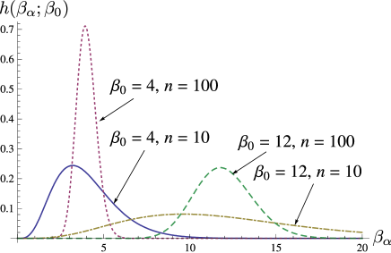
In superstatistics, three types of distribution are often used for $h(\beta_{\alpha};\beta_{0})$: the $\chi^{2}$-distribution ($\chi^{2}$-superstatistics), the log-normal distribution (log-normal superstatistics) and the inverse $\chi^{2}$-distribution (inverse $\chi^{2}$-superstatistics). The support of these distributions is $(0,\infty)$. The $\chi^{2}$-distribution is particularly important, since $\chi^{2}$ superstatistics reproduces the $q$-exponential family. As a consequence, we assume that $\beta_{\alpha}$ is sampled from the $\chi^{2}$-distribution with $n$ degrees of freedom (Fig. 4) Wilk:2000:NEXTParam ; Beck:2003:Superstatistics . The assumption of the $\chi^{2}$-distribution can be understood as follows: suppose that there are $n$ independent random processes $Y_{i}$, which are sampled from Gaussian distributions, behind $\beta_{\alpha}$. If $\beta_{\alpha}$ is realized as a sum of squared $Y_{i}$, then $\beta_{\alpha}$ is a random variable of a $\chi^{2}$-distribution with $n$ degrees of freedom. The PDF of $\beta_{\alpha}$ is given by

$$h(\beta_{\alpha};\beta_{0})=\frac{1}{\Gamma(n/2)}\left(\frac{n}{2\beta_{0}}\right)^{n/2}\beta_{\alpha}^{n/2-1}\exp\left(-\frac{n\beta_{\alpha}}{2\beta_{0}}\right),$$ (32)

where $\beta_{0}$ is a hyper-parameter, the average of $\beta_{\alpha}$. The variance of the $\chi^{2}$-distribution is given by $2\beta_{0}^{2}/n$. By substituting Eq. (32) in Eq. (31), we obtain

$$P_{st}(x)=\frac{1}{\widetilde{Z}_{B}}\left[1+\frac{2\beta_{0}}{n}\left(U(x)-U_{0}\right)\right]^{-\frac{n+1}{2}},$$ (33)

where $\widehat{Z}_{B}$ is a normalization constant. Equation (33) is a reliable solution when $\beta_{0}$ and $n$ are sufficiently large. Equation (33) can be represented by

$$P_{st}(x)=\exp_{\widetilde{q}_{B}}\left[-\ln_{2-\widetilde{q}_{B}}\widetilde{Z}_{B}-\widetilde{\beta}_{B}\left(U(x)-U_{0}\right)\right],$$ (34)

$$\widetilde{\beta}_{B}=\frac{n+1}{n}\beta_{0}\widetilde{Z}_{B}^{\widetilde{q}_{B}-1},\,\,\,\,\widetilde{q}_{B}=\frac{n+3}{n+1}.$$ (35)

Equation (34) is equivalent to Eq. (24), which indicates that superstatistical bistable stochastic processes also follow stationary distributions belonging to the $q$-exponential family.

The above calculation is carried out using Type-B superstatistics. We may alternatively calculate stationary distributions using Type-A superstatistics, where the factor of $Z(1/\beta_{\alpha})$ in Eq. (31) is neglected. This case also yields the $q$-exponential family given by Eq. (34) but with

$$\widetilde{\beta}_{A}=\beta_{0}\widetilde{Z}_{A}^{\widetilde{q}_{A}-1},\,\,\,\widetilde{q}_{A}=\frac{n+2}{n},$$ (36)

where $\widetilde{Z}_{A}$ is a normalizing constant.

III Mean First Passage Time

III.1 The Langevin Model Subjected to Quadratic Multiplicative Noise

Figure 5: (Color online) MFPTs of the Langevin model with quadratic multiplicative noise ($\kappa=2$) as functions of (a) $M$ and (b) $\widehat{q}$.

Figure 6: (Color online) The effective potentials $V(x)-V_{0}$ with $\kappa=2$.

In order to study transient properties of bistable systems, we calculate the MFPT, which is an average of the first passage time (FPT). The FPT is time required for a particle to arrive at one stable site from the other stable site.

According to Fox’s Ansatz Fox:1986:PathIntegralSDE , an analytic expression for the MFPT of $\tau$ from $x_{1}$ to $x_{2}$ is expressed by

$$\tau=\int_{x_{1}}^{x_{2}}dx\frac{1}{P_{st}(x)G(x)}\int_{-\infty}^{x}dy\,P_{st}(y),$$ (37)

where the Fokker-Plank equation of $P_{st}(x)$ is given by Eq. (13). Let $\widehat{\tau}$ be a MFPT for the quadratic multiplicative noise case. A Kramers-like formula Kramers:1940:Escape is obtained by applying the steepest descent method to Eq. (37):

$$\widehat{\tau}\simeq\frac{2\pi}{G(x_{m})\sqrt{V^{\prime\prime}(x_{1})\left|V^{\prime\prime}(x_{m})\right|}}\exp\left[V(x_{m})-V_{0}\right],$$ (38)

where $x_{m}$ is an unstable site ($x_{m}=0$) and $V_{0}:=V(x_{1})$ [$V(x)$ is given in Eq. (23)]. By substituting $V(x)$ in Eq. (38), we obtain the following expression:

$$\widehat{\tau} \simeq \frac{2\pi}{G(x_{m})\sqrt{V^{\prime\prime}(x_{1})\left|V^{\prime\prime}(x_{m})\right|}}\left[1+\frac{2M}{\kappa A}\left(U(x_{m})-U_{0}\right)\right]^{\frac{\kappa+M}{2M}}$$ (39)

$$= \frac{2\pi}{G(x_{m})\sqrt{V^{\prime\prime}(x_{1})\left|V^{\prime\prime}(x_{m})\right|}}\exp_{2-\widehat{q}}\left[\widehat{\beta}_{0}\left(U(x_{m})-U_{0}\right)\right],$$

where $\widehat{\beta}_{0}$ and $\widehat{q}$ are defined in Eq. (25), and $U_{0}=U(x_{1})$.

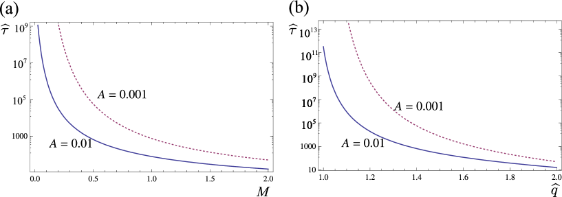
Equation (39) is a good approximation for $V(x_{m})-V_{0}\gg 1$. In the limit as $M\rightarrow 0$, Eq. (39) reduces to that for the conventional case. The last part of Eq. (39) is similar to that of the Kramers-time [Eq. (41)], with $\exp(x)$ replaced by $\exp_{2-q}(x)$. We plotted Eq. (39) in Fig. 5 ($\kappa=2$). Fig 5 (a) and (b) show MFPTs as functions of $M$ and $\widehat{q}$, respectively. In Fig. 5 (a), the MFPT decreases as the noise intensity increases. In Fig. 5 (b), it is also decreasing as a function of $\widehat{q}$. If $\kappa$ is constant, $\widehat{q}$ depends only on the multiplicative noise intensity $M$. Because $M$ is an increasing function for $1<\widehat{q}<3$, Fig. 5 (b) decreases as $\widehat{q}$ increases.

For the case of linear multiplicative noise, a Kramers-like equation is obtained over a very narrow parameter range. As can be seen in Fig. 3, the effective potentials of stationary distributions cannot be well approximated with the steepest descent method when $M$ is large.

III.2 Superstatistical Model

We next calculate the MFPT resulting from the superstatistical description. We assume that time scale of fluctuations of $\beta_{\alpha}$ is macroscopic, i.e. $\beta_{\alpha}$ does not change during each escape event. Under this assumption, the MFPT for the superstatistical case can be calculated by taking the expectation in terms of $h(\beta_{\alpha};\beta_{0})$:

$$\widetilde{\tau}=\int_{0}^{\infty}d\beta_{\alpha}\,\tau(\beta_{\alpha})h(\beta_{\alpha};\beta_{0}),$$ (40)

where $\tau(\beta_{\alpha})$ is the MFPT of the Brownian model given by Eq. (27),

$$\tau(\beta_{\alpha})\simeq\frac{2\pi}{\sqrt{U^{\prime\prime}(x_{1})\left|U^{\prime\prime}(x_{m})\right|}}\exp\left[\beta_{\alpha}\left(U(x_{m})-U_{0}\right)\right].$$ (41)

Note that Eq. (41) is the Kramers time and is valid for sufficiently large $\beta_{\alpha}$. Since the Kramers time is valid for large $\beta_{\alpha}$, we obtain the following result for sufficiently large $n$ and $\beta_{0}$:

$$\widetilde{\tau}\simeq\frac{2\pi}{\sqrt{U^{\prime\prime}(x_{1})|U^{\prime\prime}(x_{m})|}}\exp_{\widetilde{q}_{A}}\left[\beta_{0}\left(U(x_{m})-U_{0}\right)\right],$$ (42)

with $n/(2\beta_{0})>U(x_{m})-U_{0}$. We see that Eq. (42) is the same as Eq. (41), except that $\exp$ is replaced by $\exp_{q}$. For the quadratic multiplicative case, $\exp$ is replaced by $\exp_{2-q}$. We see the dual relation $q\leftrightarrow 2-q$ which often appears in nonextensive statistics. We plotted Eq. (42) in Fig. 7. Figures 7 (a) and (b) show MFPTs as functions of $\alpha_{0}:=1/\beta_{0}$ and $\widetilde{q}_{A}=(n+2)/n$, respectively. When $n\rightarrow\infty$, $\widetilde{\tau}$ reduces to the Kramers-time. Fig 7 (b) shows that the MFPT is increasing as a function of $\widetilde{q}_{A}$ (and also increasing as a function of $\widetilde{q}_{B}=(3\widetilde{q}_{A}-1)/(\widetilde{q}_{A}+1)$). As shown in Sec. III.1, the MFPT for the quadratic multiplicative case is decreasing as a function of $\widehat{q}$. It is interesting to see that effects of the entropic index on the MFPTs for both cases are inversely related, although their stationary distribution dependence on the entropic index agrees.

Figure 7: (Color online) MFPTs of the superstatistical model as functions of (a) $\alpha_{0}$ and (b) $\widetilde{q}_{A}$. For comparison, we plotted the Kramers-time in (a).

We have shown that the $q$-dependence of the MFPT in the Langevin model driven by quadratic multiplicative noise is different from that in the superstatistical model, which will be qualitatively explained as follows. In the Langevin model with quadratic multiplicative noise, larger $M$ with fixed $A$ yields a smaller MFPT (Fig. 5). Since larger $M$ leads to larger $\widehat{q}$ [Eq. (25)], the MFPT is decreasing as a function of $\widehat{q}$. On the contrary, the MFPT in the superstatistical model is expressed as superposition of MFPTs of given subsystems, in which smaller $\alpha$ (i.e. larger $\beta_{\alpha}$) leads to larger $\tau(\beta_{\alpha})$. The $\chi^{2}$-distribution with smaller $n$ (larger $\widetilde{q}_{A}$ [Eq. (36)]) has higher magnitude in large-$\beta_{\alpha}$ regions. Thus the MFPT in the superstatistical model is increasing as a function of $\widetilde{q}_{A}$, which is opposite to that in the Langevin model. However, if we adopt an effective potential $V(x)$ derived from the PDF of Eq. (33)

$$V(x)=\frac{n+1}{2}\ln\left[1+\frac{2\beta_{0}}{n}\left(U(x)-U_{0}\right)\right],$$ (43)

and substitute Eq. (43) to Eq. (38), the exponential part of Eq. (38) is given by:

$$\exp\left[V(x_{m})-V_{0}\right]=\exp_{2-\widetilde{q}_{B}}\left[\frac{n+1}{n}\beta_{0}(U(x_{m})-U_{0})\right].$$ (44)

The $q$-dependence of Eq. (44) is similar to that of the Langevin model with quadratic multiplicative noise mentioned above [Eq. (39)]. It is stressed that in order to study the MFPT (a typical dynamical quantity) in the superstatistics, it is necessary to take an average of $\tau(\beta_{\alpha})$ over $\beta_{\alpha}$ because the characteristic time of fluctuations in $\beta_{\alpha}$ is much slower than that of the MFPT.

III.3 Wall Height Dependence

We study the dependence of the MFPT on wall height (i.e. $U(x_{m})-U_{0}$). Let us consider the following functions:

$$U(x)-U_{0}=a(x^{2}-1)^{2},$$ (45)

$$g(x)=\frac{1}{2}(x^{2}-1),$$ (46)

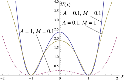
where the coefficient $a$ expresses the wall height $U(x_{m})-U_{0}$. We calculate the $a$-dependence of the MFPTs for the two statistics while keeping the noise terms unchanged. Eq. (17) with Eq. (46) is identical to Eq. (45) with $\kappa=8a$.

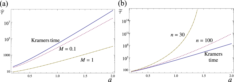
Figures 8 (a) and (b) show the wall height dependence of the MFPT for the Langevin and superstatistical models, respectively. Since Fig. 8 (a) and (b) are log-plots, the exponential dependence on $a$ is indicated by a straight line. Since the Kramers-time is dominated by an exponential of the wall height, a linear relationship is indicated in both figures (Although the Kramers-time depends on curvature of the potentials, its effect is smaller in comparison to the exponential part). Figure 8 (a) show that the log-scaled MFPT as a function of $a$ exhibits a linear relation in the Langevin model as the Kramers time. A wall height dominant part of the MFPT [Eq. (39)] for the quadratic multiplicative case is calculated as follows:

$$\exp_{2-\widehat{q}}\left[\widehat{\beta}_{0}(U(x_{m})-U_{0})\right]=\left[1+\frac{M}{4A}(x_{m}^{2}-1)^{2}\right]^{\frac{8a+M}{2M}}.$$ (47)

Eq. (47) shows the reason for the linear relation in the log-plots.

We note that the $a$-dependence of the MFPT for the superstatistical case in Fig. 8 (b) is different from that of the Langevin model in Fig. 8 (a). For $n=30$, the MFPT grows super-exponentially as a function of $a$. Equation (42) is dominated by the $q$-exponential function, and $\widetilde{q}_{A}$ is large for small $n$ ($\widetilde{q}_{A}=1.07$ for $n=30$). Although the stationary aspects are the same in some limits, their MFPTs as functions of the wall height are qualitatively different.

Figure 8: (Color online) MFPTs as a function of the wall height $a$. (a) the Langevin model with quadratic multiplicative noise and (b) the superstatistical model. In both figures, the intensity of additive noise is $A=\alpha_{0}=0.1$.

IV Discussion

IV.1 Open Quantum System

A microscopic origin for multiplicative noise was discussed for an open quantum system Barik:2005:MicroscopicMulti . It was assumed that a harmonic oscillator is coupled with harmonic oscillator bath by the interaction,

$$H_{I}=-\sum_{j}c_{j}q_{j}f(x),$$

where $x$ and $q_{j}$ denote the coordinates of the system and bath, respectively, $c_{j}$ is the coupling strength and $f(x)$ the coupling function. It has been shown that the noise term for a quantum Langevin equation in the Markovian limit is given by Barik:2005:MicroscopicMulti

$$g(x)\eta(t)=\langle f^{\prime}(x)\rangle\eta(t),$$

which yields additive [$g(x)=1$] and multiplicative noise [$g(x)=x$] for $f(x)=x$ and $f(x)=x^{2}/2$, respectively. It is possible to extend the above discussion to an open bistable quantum system which is in a stable state of either $x=x^{*}=-1$ or $+1$. The coupling interaction may be expressed as

$$H_{I}=-\sum_{j}c_{j}q_{j}f(x-x^{*}),$$

for which we obtain a multiplicative noise of $g(x)=x-x^{*}$ for $f(x-x^{*})=(x-x^{*})^{2}/2$ in the relevant quantum Langevin equation. This implies that the multiplicative noise is the most pronounced at the stable state and that it is consistent with Eq. (19) because

$$g(x)=\frac{1}{2}(x^{2}-1)\simeq(x-x^{*})\,\,\,(\mathrm{for}\,\,\,x-x^{*}\ll 1).$$

Thus our choice of $g(x)$ given by Eq. (19) is consistent with the open quantum approach Barik:2005:MicroscopicMulti .

IV.2 Effects of Correlation Between Additive and Multiplicative Noise

Figure 9: (Color online) Stationary distributions for correlated additive and quadratic multiplicative noise with each parameter setting ($\kappa=2$).

Figure 10: (Color online) Stationary distributions for correlated additive and linear multiplicative noise with each parameter setting. Results for $\lambda<0$ are given by a symmetric change of those for $\lambda>0$ with respect to the $x=0$ axis.

In many researches on bistable systems using Langevin models, the correlation between additive and multiplicative noise is considered. In such cases, the correlation function between additive and multiplicative noise is given by

$$\left\langle\xi(t)\eta(s)\right\rangle=\left\langle\eta(t)\xi(s)\right\rangle=2\lambda\sqrt{AM}\delta(t-s),$$ (48)

instead of Eq. (12). In Eq. (48), $\lambda$ represents the correlation intensity ($|\lambda|\leq 1$). The Fokker-Planck equation [Eq. (13)] is given by

$$F(x)=f(x)+\sqrt{AM}\lambda g^{\prime}(x)+Mg(x)g^{\prime}(x),$$

$$G(x)=A+2\lambda\sqrt{AM}g(x)+Mg(x)^{2}.$$

For the linear and quadratic multiplicative cases, the stationary distributions can be obtained analytically with Eq. (21) (the expressions are not shown here). We plotted the stationary distribution for correlated cases in Fig. 9 (quadratic multiplicative case) and Fig. 10 (linear multiplicative case) with $\kappa=2$. For the quadratic multiplicative case (Fig. 9), stationary distributions are symmetric for every $\lambda$. On the other hand, the linear multiplicative case results in asymmetric distributions, as shown. Furthermore, for a negative correlation region ($\lambda<0$), the stationary distributions for the linear multiplicative case are only line-symmetric distributions with respect to $x=0$. In contrast, the quadratic multiplicative noise cases yield different shapes for negative $\lambda$. Furthermore, it would be interesting to apply our method to stochastic systems with an asymmetric bistable potential which have been extensively studied in recent years Wio:1999:NonGaussSR ; Nikitin:2003:AsymPeriodic .

V Concluding Remarks

In this paper, we have investigated properties of stochastic bistable systems described by the $q$-exponential family as given by Eq. (2), using two approaches: the Langevin model driven by quadratic multiplicative noise and superstatistics. We have pointed out that quadratic multiplicative noise is more physically appropriate for bistable quartic potential systems than the linear version and that it is consistent with the result of an open quantum system Barik:2005:MicroscopicMulti . Properties of the stationary distribution for quadratic multiplicative noise are quite different from those for the linear one. We have shown that the MFPTs in the Langevin model and the superstatistical model are qualitatively different.

Langevin equations (especially the bistable cases) are widely used in biological systems, where environments fluctuate temporally and/or spatially. Recently, superstatistics has been applied to a cancer survival modeling Chen:2008:CancerSuperstatistics , and it was shown that the superstatistical description succeeded in modeling cancer survival in an accurate manner. This result indicates the importance of the superstatistical modeling for biological mechanisms. Since we only calculate here the superstatistical model for macroscopic fluctuations, it may be desirable to investigate the properties of more general cases. These are left as our future studies.

References

- (1) C. Tsallis, J. Stat. Phys. 52 (1988) 479.
- (2) C. Tsallis, in: M. Gell-Mann, C. Tsallis (Eds.), Nonextensive Entropy, Oxford University Press, 2004, p.1.
- (3) H. Suyari, M. Tsukada, IEEE Trans. Inf. Theo. 51 (2005) 753.
- (4) S. Umarov, C. Tsallis, S. Steinberg, arXiv:cond-mat/0603593v4, 2006.
- (5) A. Rodríguez, V. Schwämmle, C. Tsallis, J. Stat. Mech. (2008) P09006
- (6) C. Tsallis, Introduction to Nonextensive Statistical Mechanics: Approaching a Complex World, Springer, 2009.
- (7) Y. Hasegawa, M. Arita, Physica A 388 (2009) 3399.
- (8) J. Naudts, Entropy 10 (2008) 131.
- (9) J. Naudts, Cent. Eur. J. of Phys. 7 (2009) 405.
- (10) C. Anteneodo, C. Tsallis, J. Math. Phys. 44 (2003) 5194.
- (11) C. R. Doering, J. C. Gadoua, Phys. Rev. Lett. 69 (1992) 2318.
- (12) M. Marchi, F. Marchesoni, L. Gammaitoni, E. Menichella-Saetta, S. Santucci, Phys. Rev. E 54 (1996) 3479.
- (13) R. N. Mantegna, B. Spagnolo, Phys. Rev. Lett. 76 (1996) 563.
- (14) B. Spagnolo, N. Agudov, A. A. Dubkov, arXiv:cond-mat/0405392v1, 2004.
- (15) G. Wilk, Z. Włodarczyk, Phys. Rev. Lett. 84 (2000) 2770.
- (16) C. Beck, E. G. D. Cohen, Physica A 322 (2003) 267.
- (17) C. Beck, Braz. J. Phys. 39 (2009) 357.
- (18) R. F. Rodríguez, I. Santamaría-Holek, Physica A 385 (2007) 456.
- (19) P. Mazur, Physica A 274 (1999) 491.
- (20) P. Jizba, H. Kleinert, Phys. Rev. E 78 (2008) 031122.
- (21) S. L. Heston, Rev. Financ. Stud. 6 (1993) 327.
- (22) C. Beck, Prog. Theo. Phys. 162 (2006) 29.
- (23) S. Martínez, F. Nicolás, F. Pennini, A. Plastino, Physica A 286 (2000) 489.
- (24) F. Sattin, Eur. Phys. J. B 49 (2006) 219.
- (25) R. F. Fox, Phys. Rev. A 33 (1986) 467.
- (26) H. A. Kramers, Physica VII 4 (1940) 284.
- (27) D. Barik, D. S. Ray, J. Stat. Phys. 120 (2005) 339.
- (28) H. S. Wio, S. Bouzat, Braz. J. Phys. 29 (1999) 136.
- (29) A. Nikitin, N. G. Stocks, A. R. Bulsara, Phys. Rev. E 68 (2003) 016103.
- (30) L. L. Chen, C. Beck, Physica A 387 (2008) 3162.