A Bootstrap Algebraic Multilevel method for Markov Chains

Abstract.

This work concerns the development of an Algebraic Multilevel method for computing stationary vectors of Markov chains. We present an efficient Bootstrap Algebraic Multilevel method for this task. In our proposed approach, we employ a multilevel eigensolver, with interpolation built using ideas based on compatible relaxation, algebraic distances, and least squares fitting of test vectors. Our adaptive variational strategy for computation of the state vector of a given Markov chain is then a combination of this multilevel eigensolver and associated multilevel preconditioned GMRES iterations. We show that the Bootstrap AMG eigensolver by itself can efficiently compute accurate approximations to the state vector. An additional benefit of the Bootstrap approach is that it yields an accurate interpolation operator for many other eigenmodes. This in turn allows for the use of the resulting AMG hierarchy to accelerate the MLE steps using standard multigrid correction steps. Further, we mention that our method, unlike other existing multilevel methods for Markov Chains, does not employ any special processing of the coarse-level systems to ensure that stochastic properties of the fine-level system are maintained there. The proposed approach is applied to a range of test problems, involving non-symmetric stochastic M-matrices, showing promising results for all problems considered.

1. Introduction

We consider the task of computing a non-zero vector $x$ such that

(1) $$Ax=1\,x,$$

where $A$ denotes the transition matrix of a given irreducible Markov process and $x$ is the associated state vector, an eigenvector of $A$ with eigenvalue equal to one. Since $A$ is irreducible, $x$ is unique up to scalar factors. The approach considered in this paper is to approximate $x$ iteratively using an Algebraic Multigrid (AMG) method designed to find a non-trivial solution to the eigenvalue problem

$$Bx=0\,x,\enspace\mbox{{\color[rgb]{0,0,0}where $B=I-A$,}}$$

in the setup phase and use the computed AMG method to solve the homogeneous system

$$Bx=0,$$

. Our AMG algorithm relies on the Bootstrap framework, a fully adaptive algebraic multigrid scheme proposed in [4]. For solving complex-valued linear systems, this BootAMG (Bootstrap AMG) framework was efficiently put into action in [6]. In this paper, we develop a variant of BootAMG specifically tailored to compute $x$ in (1). Although we are not (yet) in a position to give a full rigorous mathematical analysis of the method, we demonstrate the efficiency of the BootAMG approach for a series of Markov Chain test problems.

The main new ingredient of our BootAMG method is an adaptive (setup) component that simultaneously computes an approximation to the state vector and Test Vectors (TVs) which are then used in a Least Squares approach to calculate a multilevel sequence of interpolation operators. Letting $\ell$ denote a given level of the multilevel hierarchy and taking on the finest level $B_{0}=B$, our adaptive strategy consists of the following steps (explained and described in detail in the latter sections):

1. relax on the homogeneous system $B_{\ell}x_{\ell}=0,B_{\ell}\in\mathbb{R}^{n_{\ell}\times n_{\ell}}$ to improve the set of test vectors, $x^{(1)}_{\ell},...,x^{(r)}_{\ell}$, approximating the state vector; $n_{\ell}$ here is the problem size on level $\ell$;

2. compute a sparse interpolation operator $P_{\ell}\in\mathbb{R}^{n_{\ell+1}\times n_{\ell}}$ using a least-squares fit based on $x^{(1)}_{\ell},...,x^{(r)}_{\ell}$;

3. compute the system matrix $B_{\ell+1}\in\mathbb{R}^{n_{\ell+1}\times n_{\ell+1}}$ on the next coarser level as $B_{\ell+1}=Q_{\ell}B_{\ell}P_{\ell}$ via a Petrov-Galerkin approach, with the restriction $Q_{l}\in\mathbb{R}^{n_{\ell}\times n_{\ell+1}}$ representing a simple averaging operator; also calculate the mass matrix $T_{l+1}=Q_{\ell}T_{\ell}P_{\ell}$ (with $T_{0}=I$) for the next leg of BootAMG;

4. obtain the coarse-level series of test vectors

   $$x^{(j)}_{\ell+1}=R_{\ell}x^{(j)}_{l},\ j=1,...,r,\quad\text{with\ }R_{\ell}\in\mathbb{R}^{n_{l+1}\times n_{l}}\quad\text{being injection}.$$

This process is applied recursively until a level with sufficiently small problem size (the coarsest level, $\ell=L$) is reached. There, an exact eigensolve for

$$B_{\ell}x=\lambda T_{\ell}x$$

is performed and then used to improve the given approximations to the state vector on increasingly finer levels. Along with the state vector’s approximations $x^{(0)}_{\ell}$, some (small number) of near kernel eigenfunctions $(\lambda_{i},x^{(i)}_{\ell})$, from the coarsest level are interpolated to increasingly finer levels, where they are relaxed and then used as initial guesses to the corresponding fine-level eigenvectors. On each such level, the relaxation is performed on the homogeneous system

$$(B_{\ell}-\lambda_{i}T_{\ell})x^{(i)}_{\ell}=0,$$

and the approximations to $\lambda_{i}$ are updated (except for $\lambda_{0}$ which is known to be exactly zero.) Each $x^{(i)}_{\ell}$ is already a reasonable approximation to an eigenfunction on level $\ell$, i.e,

$$B_{\ell}x^{(i)}_{\ell}\approx\lambda_{i}^{\ell}T_{\ell}x^{(i)}_{\ell}$$

for an $\ell^{th}$ level eigenvalue $\lambda_{i}^{\ell}$. Therefore, a good eigenvalue approximation can be obtained by

$$\hat{\lambda}_{i}=\displaystyle\frac{(B_{\ell}x^{(i)}_{\ell},v)}{(T_{\ell}x^{(i)}_{\ell},v)}$$

for any vector $v$. We choose $v=x^{(i)}_{\ell}$ and thus calculate an approximation to eigenvalue using what would be a Rayleigh quotient for Hermitian matrices. The change in eigenvalue approximation for each vector $x^{(i)},\,i>1$ after relaxation provides a measure of their accuracy – if after relaxation the relative change is significant, we add $x^{(i)}$ to the set of test vectors. Otherwise, these eigenvectors are well approximated by the existing interpolation operator to the current level and thus need not be built into the related coarser space. The state eigenvector approximation is always included in the test set. After all test sets on all levels, including the finest, are updated, all $P_{\ell}$, $B_{\ell}$, and $T_{\ell}$ are recalculated, and the setup stage is complete.

Once the adaptive setup is finished, we use the resulting V-cycle AMG method as a preconditioner to (full) GMRES, applied to the homogeneous system $Bx=0$. This iteration converges rapidly to the state vector, since as we demonstrate later, the BootAMG preconditioner efficiently separates the state vector from the field of values of $B$ on an appropriate complementary subspace. This use of both MLE steps and V-cycle preconditioned GMRES iterations is the other main new idea in the present paper.

The remainder of this paper is organized as follows. Section 2 contains an introduction to Markov chain systems and a general review of AMG approaches for computing state vectors of Markov chains. Section 3 contains a general description of the Bootstrap AMG ideas along with full algorithmic descriptions of realizations that we use in this paper. In Section 4 we discuss our BootAMG algorithm for Markov chains and theory for our AMG-GMRES solver. Numerical experiments are presented in Section 5 and concluding remarks are given in Section 6.

2. Overview of Solvers for Markov Chain Systems

The transition matrix $A\in\mathbb{R}^{n\times n}$ of a Markov process contains as its entries $a_{ij}$, the transition probabilites from state $i$ to state $j$, $a_{ij}\geq 0$ for all $i,j$. Matrix $A$ is column stochastic, i.e. $A^{t}\mathbf{1}=\mathbf{1}$, with $\mathbf{1}$ being the vector of all ones. It is always possible to eliminate self-transitions [19], so we assume $a_{ii}=0$ for all $i$ from now on. The state vector $x$ satisfies

$$Ax=x$$

with $x\neq 0$, $0\leq x_{i}$. By the Perron-Frobenius theorem (cf. [1, p. 27], e.g.) such a vector $x$ always exists.

A general square matrix $A\in\mathbb{R}^{n\times n}$ induces a directed graph $G(A)=(V,E)$ with vertices $V=\{1,\ldots,n\}$ and directed edges $E=\{(i,j)\subset V^{2}:i\neq j\mbox{ and }a_{ij}\neq 0\}$. Two vertices $i$ and $j$ in $G(A)$ are said to be strongly connected (as in graph theory) if there exist directed paths in $G(A)$ from $i$ to $j$ and from $j$ to $i$. Since this is an equivalence relation on the vertices, it induces a partitioning of $V$ into the strong components of $G(A)$. If $G(A)$ has exactly one strong component, the matrix $A$ is called irreducible; otherwise it is called reducible which is precisely the case when there exists a permutation matrix $\mathcal{P}$ such that

$$\mathcal{P}^{t}A\mathcal{P}=\begin{pmatrix}A_{11}&0\\ A_{12}&A_{22}\end{pmatrix},$$

where $A_{11}$ and $A_{22}$ are square submatrices.

If $A$ is irreducible — which we assume throughout — the Perron-Frobenius Theorem guarantees that the state vector $x$ has all positive values and is unique up to a scalar factor. From this theorem it also follows that the spectral radius of $A$ satisfies $\rho(A)=1$, implying that $B=I-A$ is a singular $M$-matrix; recall that $0\leq a_{ij}\leq 1$. In addition, $B$ is irreducible, because of the irreducibility of $A$.

The idea of using Multigrid (MG) to compute the state vector of an irreducible transition matrix is not new. Numerous approaches have been explored in the past, in both the aggregation-based [10, 11, 20, 21] and Classical [23] MG settings. In [20], the idea of using a partition of unity type aggregation method was first explored. Later, in [10], an extension of this approach based on Smoothed Aggregation was developed for application to the page rank problem and further generalized in [11]. For an overview of Classical MG type methods (and preconditioners) we direct the reader to [23] and the references therein.

Our MG solver can be loosely categorized as a variation of the Classical AMG approach in the following way. We choose the coarse level variables as a subset of the fine level variables. In this aspect, our approach is most closely related to the recent work by Virnik [23]; we too employ the AMG-type method as a preconditioner for GMRES. Our proposed new approach, however, differs from all previous AMG-type solvers for Markov chains in several ways. Most importantly, we build interpolation adaptively using a Least Squares approach, and we combine the multilevel eigensolver with application of correction steps using an AMG-GMRES preconditioner. Unlike other methods, we thus (experimentally) observe an excellent convergence without the need to recompute interpolation and the entire coarse-level hierarchy at each iteration. In addition, our solver yields an efficient and straightforward method for Markov chains which computes the state vector to arbitrary accuracy without the need for lumping (see [11]) and other such approaches typically employed to maintain the stochastic properties of the transition matrix and state vectors on all coarse levels of the MG hierarchy.

3. Bootstrap AMG

In this section, we provide a general review of the Bootstrap AMG framework [4, 7] for building MG interpolation together with some heuristic motivation of our choices for the individual components of the BootAMG multigrid algorithm.

The first key ingredient to any AMG method is its relaxation or smoothing iteration. For a given system matrix $B$ it is a splitting based iteration

(2) $$Mu^{\nu+1}=Nu^{\nu}+b,\enspace\mbox{ where }B=M-N,\,M\mbox{ non-singular},\,\nu=0,1,\ldots$$

with its “error propagation matrix” given by $M^{-1}N=I-M^{-1}B$. Here, $M$ is chosen such that after a few iterations the error $e^{\nu}$ w.r.t. the solution of $Bx=b$ is algebraically smooth, i.e. $\|Be^{\nu}\|\ll\|e^{\nu}\|$. In many situations this can be achieved by point-wise Gauss-Seidel or (under-relaxed) Jacobi iterations. Indeed, in our Markov chain setting we used $\omega$-Jacobi relaxation with $\omega={\color[rgb]{0,0,0}0.7}$ on all levels, i.e., we took $M=\frac{1}{\omega}\mbox{diag}(B)$, resulting in $I-M^{-1}B=I-\omega\cdot(\mbox{diag}(B))^{-1}B$.

(In case a diagonal entry $b_{ii}$ of $B$ happens to be zero for some row(s) $i$, Kaczmarz or some other distributive relaxation scheme can be applied to the $i^{th}$ equation.)

The Bootstrap AMG process can now be described as follows. Coarse variables are selected as a subset of the fine variables using a full coarsening (for problems on structured grids) or, otherwise, compatible relaxation (CR) coarsening scheme [3]. The CR scheme can be either started from scratch, or, if geometric information is given and a suitable candidate set of coarse variables is known, such set can be tested and improved by CR. Interpolation is then computed using a Least Squares based approach. We mention that once a tentative Multigrid hierarchy has been defined, it can be used to further enhance the set of test vectors.

3.1. Choosing the coarse variables: compatible relaxation

In the AMG setting, CR is a relaxation-based coarsening process which can be viewed as a special case of a general approach for constructing coarse-level descriptions of given fine-level systems, including non-stationary, highly non-linear, and also non-deterministic systems [5]. The basic idea of CR is to use the given relaxation scheme (2), restricted to appropriately defined subspaces, to measure the quality of the given coarse space and also to iteratively improve it if needed. We proceed with a brief overview of CR and its use in AMG coarsening. A detailed discussion, theory and comparisons between various measures of the quality of coarse spaces and their relations to compatible relaxation schemes are presented in [3, 8, 9, 12, 13, 16].

3.1.1. Classical AMG CR-based coarsening

Assume that the set of coarse-level variables, $\mathcal{C}$, is a subset of the set of fine-level variables, $\Omega$. Under this assumption, one possible form of CR is given by $\mathcal{F}$-relaxation for the homogeneous system — relaxation applied only to the set of $\mathcal{F}$ variables, with $\mathcal{F}:=\Omega\setminus\mathcal{C}$. Given the partitioning of $\Omega$ into $\mathcal{F}$ and $\mathcal{C}$, we have

$$u=\begin{pmatrix}u_{f}\\ u_{c}\end{pmatrix},\enspace B=\begin{pmatrix}B_{ff}&B_{fc}\\ B_{cf}&B_{cc}\end{pmatrix},\enspace\mbox{and}\enspace M=\begin{pmatrix}M_{ff}&M_{fc}\\ M_{cf}&M_{cc}\end{pmatrix},$$

assuming the equations are permuted such that the unknowns in $\mathcal{F}$ come before those in $\mathcal{C}$. The $\mathcal{F}$-relaxation of CR is then defined by

(3) $$u_{f}^{\nu+1}=(I-M_{ff}^{-1}B_{ff})u_{f}^{\nu}=E_{f}u_{f}^{\nu}.$$

If $M$ is symmetric, the asymptotic convergence rate of CR

$$\rho_{f}=\rho(E_{f}),$$

where $\rho$ denotes the spectral radius, provides a measure of the quality of the coarse space, that is, a measure of the ability of the set of coarse variables to represent error not eliminated by the given fine-level relaxation. This measure can be approximated using $\mathcal{F}$-relaxation for the homogeneous system with a random initial guess $u_{f}^{0}$. Since $\lim_{\nu\to\infty}\|E_{f}^{\nu}\|^{1/\nu}=\rho(E_{f})$ for any norm $\|\cdot\|$, the measure

(4) $$\left(\|u_{f}^{\nu}\|/\|u_{f}^{0}\|\right)^{1/\nu}$$

estimates $\rho_{f}$.

In choosing $\mathcal{C}$, we use the CR-based coarsening algorithm developed in [9]. This approach is described in Algorithm 1.

Algorithm 1 compatible_relaxation {Computes $\mathcal{C}$ using Compatible Relaxation}

  Input: $\mathcal{C}_{0}$ {$\mathcal{C}_{0}=\emptyset$ is allowed}

  Output: $\mathcal{C}$

  Initialize $\mathcal{C}=\mathcal{C}_{0}$

  Initialize $\mathcal{N}=\Omega\setminus\mathcal{C}$

  Perform $\nu$ CR iterations (3) with components of $u^{0}$ randomly generated

  while $\rho_{f}>\theta$ do

     $\mathcal{N}=\{i\in\Omega\setminus\mathcal{C}:\frac{\displaystyle|u_{i}^{\nu}|}{\displaystyle|u_{i}^{\nu-1}|}>\theta\}$

     $\mathcal{C}=\mathcal{C}\cup\{\text{independent set of\ }\mathcal{N}\}$

     Perform $\nu$ CR iterations (3) with components of $u^{0}$ randomly generated

  end while

In our numerical experiments for Markov chains, we use weighted Jacobi CR, set the CR tolerance $\theta=.85$, the number of CR sweeps $\nu=8$, choose the components of $u^{0}$ to be uniformly distributed in the interval $[1,2]$, and select $\mathcal{C}_{0}$ using the standard independent set algorithm (see [22]) based on the full graph of the system matrix. For further information on CR we refer the reader to [9].

3.2. Building Bootstrap AMG interpolation

We now outline the Least Squares (LS) approach for defining interpolation, see also [6]. We assume that the set ${\mathcal{C}}$ of coarse variables is given, i.e., it has been previously determined, for instance, by geometric coarsening and/or using compatible relaxation. In the LS approach, the interpolation operator $P$ is chosen to approximate a given (specifically chosen) set of test vectors. We define $c$ as the maximum number of coarse-level variables used to interpolate to a single fine-level variable, or equivalently the maximum number of non-zero entries in any row of $P$. The key ingredient of the BootAMG setup lies in the use of several test vectors (TVs) that collectively should represent those error components not reduced by relaxation. We assume for now that such a set of test vectors, $\mathcal{U}:=\{x^{(k)}\}_{k=0}^{r}$ is known on some fine level. The rows of the prolongation operator $P$ are then obtained individually. For each variable $i\in\mathcal{F}$, we first determine a set of its neighboring coarse-level variables, $\mathcal{N}_{i}$, using the directed graph $G(A)$

(5) $$\mathcal{N}_{i}=\{j\in\mathcal{C}:\mbox{ there is a path of length $\leq z$ in $G(A)$ from $i$ to $j$ }\},$$

where $z\leq 3$, such that $\mathcal{N}_{i}$ is a subset of the local graph neighborhood of $i$. We then determine an appropriate set of (coarse level) interpolatory variables $\mathcal{J}_{i}\subseteq\mathcal{N}_{i}$ with $|\mathcal{J}_{i}|\leq c$ that yields the best fit of the LS interpolation for point $i\in\mathcal{F}$. For ease of presentation let us use the indices $j\in\mathcal{J}_{i}$ of the fine level variables to address the columns of $P$. We then define the local least squares functional for the nonzero entries $P_{i}=\{p_{ij}:j\in\mathcal{J}_{i}\}$ of row $i$ of $P$ as

(6) $$L(P_{i};\mathcal{J}_{i})=\sum_{k=0}^{r}\omega_{k}\left(x_{i}^{(k)}-\sum_{j\in\mathcal{J}_{i}}p_{ij}{\color[rgb]{0,0,0}x}_{j}^{(k)}\right)^{2}.$$

The task is then to find a set $\mathcal{J}_{i}$ of interpolating points for which the minimum of $L$ is small and to obtain the corresponding values $p_{ij}$ of the minimizer that yield the coefficients for the interpolation operator. Generally, the weights $\omega_{k}$ should be chosen according to the algebraic smoothness of $x^{(k)}$ to bias the least squares functional towards the smoothest vectors. We do so by using the square of the inverse of the norm of the residual of the homogeneous problem $B_{\ell}x^{(k)}=0$ for each $x^{(k)}$.Here $\ell$ is the current level to which operator $P$ interpolates from the next coarser level $\ell+1$.

Our approach for solving this task is given as Algorithm 2. It is based on a greedy strategy to find an appropriate set of interpolatory points $\mathcal{J}_{i}$ for each fine point $i$; see [6] and [15].

Algorithm 2 ls_interpolation {Computes Least Squares based interpolation}

  Input: $\mathcal{U}$, $c$

  Output: interpolation $P$

  $X^{(k)}=R\,x^{(k)},x^{(k)}\in\mathcal{U}$

  for $i\in\mathcal{F}$ do

     Take $\mathcal{N}_{i}$ from (5)

     Set $\mathcal{J}_{i}=\emptyset$

     repeat

        determine $g^{*}\in\mathcal{N}_{i}$ s.t. $\underset{P_{i}}{\min}\,L(P_{i};\mathcal{J}_{i}\cup\{g^{*}\})=\underset{g\in\mathcal{N}_{i}}{\min}\,\underset{P_{i}}{\min}\,L(P_{i},\mathcal{J}_{i}\cup\{g\})$

        Set $\mathcal{N}_{i}=\mathcal{N}_{i}\setminus\{g^{*}\}$ and $\mathcal{J}_{i}=\mathcal{J}_{i}\cup\{g^{*}\}$

     until $|\mathcal{J}_{i}|\geq c$ or $\mathcal{N}_{i}=\emptyset$

  end for

4. MLE and AMG-GMRES Algorithms

In this section, we discuss the main ideas and their implementations in our BootAMG-based algorithm for computing non-trivial solutions $x$ to $Bx=0$, where as before $B=I-A$, $A$ is an irreducible column stochastic transition matrix so that $B$ is a non-symmetric and singular $M$-matrix. The goal of each MLE step is twofold: (1) to compute approximations to the solution $x$ and also to compute suitable test vectors that allow us to improve the accuracy of Least Squares interpolation and (2) to update the multigrid hierarchy, used to precondition GMRES.

Such a hierarchy consists of a sequence of prolongation and restriction operators and systems of coarse-level equations. The coarse-level equations are defined using the Petrov-Galerkin approach. More precisely, $B_{l+1}=Q_{l}B_{l}P_{l}$, with restriction $Q_{l}$ given by the averaging operator. This means that each column of $Q_{l}$ has identical nonzero entries at exactly the positions corresponding to $\mathcal{J}_{i}$ and that $\mathbf{1}^{t}Q_{l}=\mathbf{1}^{t}$. This implies $B_{l}^{t}\mathbf{1}=\mathbf{0}$ for all levels $l$.

4.1. Multilevel Eigensolver (MLE)

Our approach for building a multilevel method relies on the BootAMG framework. We construct a sequence of increasingly coarser-level descriptions of the given fine-level Markov Chain system using the LS-based fit discussed above. The coarse-level test vectors are calculated from the fine-level test set as $X^{(k)}=Rx^{(k)}$. On the coarsest level, the eigenproblem is solved exactly for some small number of the lowest (in absolute value) eigenvectors, which are then directly interpolated and relaxed on finer levels, becoming increasingly more accurate approximations to the finest-level eigenfunctions (such treatment is similar to the Exact Interpolation Scheme, e.g, [17]). These eigenfunction approximations are added to test sets on each level. Note that the initial (random) test functions are not relaxed during this stage – otherwise they may become almost linearly dependent which may result in ill-posed local least squares problem. With the improved TV sets (enriched by eigenfunction approximations), new prolongation operators are then calculated.

We note that the setup cycle in Algorithm 3 also yields an approximation to the state vector which we use as an initial guess in our AMG-GMRES iterations. This approach can also be used as a stand-alone solver for these systems although, in general, it will be far more expensive than using several AMG-GMRES steps in addition to the MLE. We note that for certain problems (e.g., when several eigenvalues of $B$ are close to zero) and for larger problem sizes, it may be necessary to alternate several times between the MLE and AMG-GMRES iterations to find an accurate approximation of $x$. In our tests, we found it sufficient to use either a traditional $V$-cycle ($\mu=1$) or $W$-cycle ($\mu=2$) for the MLE step followed by a small number of AMG-GMRES steps to compute an approximation to the state vector. Ultimately, in our MLE approach, the sequence of prolongation operators needs to be accurate for only the smoothest error component – the kernel of the finest-level operator $B=I-A$. The accurate resolution of many other near-kernel components by our LS-based interpolation operator allows for fast convergence of MG preconditioned GMRES, whereas the kernel component of $B$ is the state vector we aim to compute. Algorithm 3 contains a pseudo-code of our implementation of the MLE iteration.

Algorithm 3 bootamg_mle {Implements the Bootstrap AMG MLE scheme}

  Input: $B_{l}$ ($B_{0}=B$), $T_{l}$, ($T_{0}=I$), $\mathcal{U}_{l}$ (set of test vectors on level $l$)

  Output: updated $\mathcal{U}_{l}$ and $(\Lambda_{l},\mathcal{V}_{l})$, approximations to the lowest eigenpairs;

  if $l=L$ then

     Compute $\mathcal{V}_{L}=\{x^{(i)}\}_{1,\ldots,k}$, s.t. $B_{L}x^{(i)}=\lambda^{(i)}T_{L}x^{(i)},|\lambda^{(1)}|\leq|\lambda^{(2)}|\leq\ldots\leq|\lambda^{(k)}|$.

  else

     Relax $B_{l}x^{(j)}=0,\ x^{(j)}\in\mathcal{U}_{l}$

     Set $\mathcal{V}_{l}=\emptyset$

     for $m=1,\ldots,\mu$ do

        $P_{l}=\mbox{ls\_interpolation}(\mathcal{U}_{l}\cup\mathcal{V}_{l},c)$

        Compute averaging $Q_{l}$ with $\mbox{sparsity}(Q_{l})=\mbox{sparsity}(P_{l})$

        $B_{l+1}=Q_{l}B_{l}P_{l}$

        $T_{l+1}=Q_{l}T_{l}P_{l}$

        $\mathcal{U}_{l+1}=\{R_{l}x,x\in\mathcal{U}_{l}\}$

        $\mathcal{V}_{l+1}=\mbox{bootamg\_mle}(B_{l+1},T_{l+1},\mathcal{U}_{l+1})$

        ${\mathcal{V}}_{l}=\{P_{l}x,x\in\mathcal{V}_{l+1}\}$

        for $i=1,\ldots,|{\mathcal{V}}_{l}|$ do

           Relax $(B_{l}-\lambda_{i}T_{l})x^{(i)}=0$, $x^{(i)}\in\mathcal{V}_{l}$

           Update ${\lambda}_{i}=\displaystyle\frac{\langle B_{l}x^{(i)},x^{(i)}\rangle}{\langle T_{l}x^{(i)},x^{(i)}\rangle}$

        end for

     end for

  end if

In Figure 1 a possible setup cycle is visualized. We note that at each square one has to decide whether to recompute $P$ or advance to the next finer grid in the multigrid hierarchy. The illustrated cycle resembles a $W$-cycle, but any other cycling strategy can be applied to the setup.

Figure 1. Bootstrap AMG setup W-cycle.

4.2. Multigrid preconditioned GMRES

The multilevel eigensolve steps described above yield increasingly better approximations to the state vector and other vectors that cannot be removed efficiently by the Multigrid relaxation.

Although we are only interested in computing the state vector, the LS-based Multigrid hierarchy is able to resolve a larger subspace. This leads to the idea of exploiting this richness of the given hierarchy for use in MG correction steps – in addition to the discussed MLE steps.

To illustrate the effect of MG correction steps applied to the homogeneous problem $Bx=0$, we start by analyzing simple relaxation schemes for the steady state problem, $Ax=x$. As the steady state solution is the eigenvector corresponding to the eigenvalue with largest absolute magnitude, a power iteration

(7) $$x^{k+1}=Ax^{k}$$

is guaranteed to converge to the solution. However, convergence can be slow if $A$ has other eigenvalues with absolut value close to one.

Such power iterations applied to the steady state problem are in turn equivalent to applying a Richardson iteration to the homogeneous system $\left(I-A\right)x=0$. A natural modification, facilitating that the field of values of $A$ is contained in the unit circle, is then given by a suitable under-relaxed iteration, yielding the error propagator

(8) $$e^{k+1}=\left(I-\tau B\right)e^{k}.,$$

which translates into an identical relation for the iterates,

(9) $$x^{k+1}=\left(I-\tau(I-A)\right)x^{k},$$

so that the iteration can be interpreted as a modified power method.

In Figures 2(a) and 2(b) the spectra of $A$ and of $I-\tau\left(I-A\right)$ are depicted for a characteristic two-dimensional test problem, along with the field of values. The error propagator of the MG V-cycle applied to $Bx=0$ is given by

(10) $$E=\left(I-MB\right)\left(I-P{E_{c}}QB\right)\left(I-MB\right),$$

where ${E_{c}}$ denotes the error propagation operator on the next coarser level. This recursive definition terminates at the coarsest level with $E=B^{\dagger}$, the Moore-Penrose inverse of the matrix on the coarsest level, since we compute the minimal norm solution of the respective system at that level. The error propagator can be rewritten as

(11) $${\color[rgb]{0,0,0}I-\mathcal{C}B},$$

so that comparing with the one from (8) (relaxed Richardson) we see that we can interprete the multigrid V-cycle as yet another modification of the power iteration. In Figure 2(c), the spectrum and field of values of the MG V($2,2$)-cycle preconditioned matrix (11) is depicted. For this case, it is clear that applying power iterations to this preconditioned operator will converge rapidly to the steady state vector.

(a) Spectrum and field of values for Richardson error propagator.

(b) Spectrum and field of values for $\tau$-Richardson.

(c) Spectrum and field of values of Multigrid error propagator.

Figure 2. Spectra and field of values of the Richardson, $\tau$-Richardson and Multigrid error propagators for two-dimensional tandom queuing problem with $n=33^{2}$.

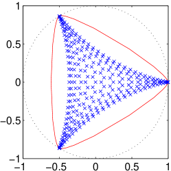
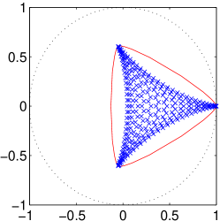
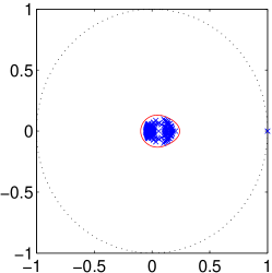
To further accelerate this approach, instead of the straightforward power method, we consider MG preconditioned GMRES steps. As we show below, such iteration is guaranteed to converge to the solution of our Markov Chain systems.

Remark 4.1.

Let $A$ be a column-stochastic irreducable operator and $B=I-A$. Then we have

(12) $$\mbox{range}\left(B\right)\cap\mbox{null}\left(B\right)=\{0\}.$$

Proof.

As $A$ is column-stochastic we know that $A^{t}\mathbf{1}=\mathbf{1}$. Hence $B^{t}\mathbf{1}=0$. Furthermore we know from the Perron-Frobenius theorem that $Bx=0$ is uniquely solvable up to a scalar factor and the solution $x^{*}$ is strictly positive (component-wise). Thus, as for all $y\in\mbox{range}\left(B\right)$ there exists a $z$ such that $y=Bz$ we have $\langle\mathbf{1},y\rangle=\langle\mathbf{1},{\color[rgb]{0,0,0}Bz}\rangle=\langle{\color[rgb]{0,0,0}B^{t}}\mathbf{1},z\rangle=0$. With this and $\langle\mathbf{1},x^{*}\rangle\neq 0$ as $x^{*}$ is strictly positive we get (12). ∎

In [14, Theorem 2.8] it is shown that GMRES determines a solution of $Bx=b$ for all $b\in\mbox{range}\left(B\right),x_{0}\in\mathbb{R}^{m}$ iff $\mbox{range}\left(B\right)\cap\mbox{null}\left(B\right)=\{0\}$. Due to Lemma 4.1 the assumptions of this theorem are fulfilled for $B=I-A$, where $A$ is a column-stochastic irreducible operator arising in Markov-Chain models. There seems to be no simple way to extend Lemma 4.1 to the multigrid preconditioned matrix. So the observation that GMRES for the multigrid preconditioned matrix worked out very well in all our experiments is not backed by theory so far.

4.3. A multigrid preconditioned Arnoldi method

Instead of solving the homogeneous linear system with preconditioned GMRES, we can also perform the Arnoldi method for the preconditioned matrix $\mathcal{C}B$. We thus compute orthonormal vectors $v_{1},v_{2},\ldots$ in the usual way such that $v_{1},\ldots,v_{k}$ is a basis of the Krylov subspace $\mbox{span}\{y,\mathcal{C}y,\ldots,(\mathcal{C}B)^{k-1}y\}$. Denoting $H_{k}\in\mathbb{R}^{k\times k}$ the orthogonal projection of $\mathcal{C}B$ onto the Krylov subspace, i.e. $H_{k}=V_{k}^{t}(\mathcal{C}B)V_{k}$ with $V_{k}=[v_{1}|\ldots|v_{k}]$, we compute the eigenvalue closest to 0 of $H_{k}$ and the corresponding eigenvector $\eta$. We then take the Ritz vector $V_{k}\eta$ as an approximation for the steady state vector. For the vector $y$ upon which we build the Kryolv subspace we take the approximation $x$ for the steady state vector resulting from the MLE setup phase.

5. Numerical Results

In this section, we provide results obtained using our Bootstrap AMG method when applied to a series of Markov Chains. Our numerical tests consist of our BootAMG-based approach to three Markov chain models that can be represented by planar graphs. Each of the models has certain interesting characteristics that pose problems for the solver.

5.1. Test Problems

We begin our experiments with a very simple model. The uniform two-dimensional network can be seen as the Markov chain analogue of the Laplace operator. It is defined on an equidistant grid $\Omega$ of size $N\times N$. We denote this grid in graph notation as $G_{\Omega}=(V_{\Omega},E_{\Omega})$. The entries of $A$ are then given as

$$a_{i,j}=\left\{\begin{array}[]{cl}\frac{1}{d_{out}(j)},&\text{if\ }(i,j)\in E_{\Omega}\\ 0,&\text{otherwise},\end{array}\right.$$

where $d_{out}(j)$ is the number of outgoing edges of $j\in\Omega$. In Figure 3, we illustrate the two-dimensional uniform network problem.

Figure 3. Uniform network model on a two-dimensional equidistant grid.

In the tests we conduct, we use again full-coarsening, i.e., we choose $\mathcal{C}$ to be every other grid point in both spatial dimensions. In order to keep the overall invested work small, we consider to take only up to two interpolatory points $\mathcal{C}_{i}$ per point $i\in\mathcal{F}=\Omega\setminus\mathcal{C}$. As the steady-state vector is known to be strictly positive, we choose to use initially random, but positive test vectors for this first problem, and also in all following tests. More precisely, we choose vectors with entries uniformly distributed in $[1,2]$.

In Table 1, we present results that use $6$ test vectors and a $V(2,2)$-cycle MLE step with $\omega$-Jacobi smoother, $\omega=.7$. We report the number of iterations needed to compute the steady-state vector $x$, such that

$$\|Bx\|\leq 10^{-8},\|x\|=1.$$

In addition, the number of preconditioned GMRES iterations needed to achieve the same accuracy is reported, with the initial MLE setup cycle denoted by the subscript. The coarsest grid in the experiments is always $5\times 5$.

$N$	17	33	65	129
MLE	$10$	$9$	$10$	$11$
pGMRES	$7_{V}$	$8_{V}$	$10_{V}$	$10_{V^{2}}$
pArnoldi	$7_{V}$	$8_{V}$	$10_{V}$	$9_{V^{2}}$

Table 1. Multilevel results for the two-dimensional uniform network model on an $N\times N$ grid. We report results to compute the steady-state vector $x$ to an accuracy of $10^{-8}$, using a $V(2,2)$-MLE cycle with $\omega$-Jacobi smoothing, $\omega=.7$. In addition we also report the number of iterations pGMRES needs to achieve the same accuracy, where we denote the initial bootstrap setup in the subscript. The sets $\mathcal{U}$ and $\mathcal{V}$ consist of $6$ initially positive random vectors and coarsest grid eigenvectors, respectively.

The operator complexity in these tests is bounded by $1.6$. The test shows that the MLE scales with increasing problem-size, while the number of preconditioned GMRES iterations grows slightly. However, one step of pGMRES is much cheaper than one step of MLE. Although we do not report results here, in general we may also consider restarting the MLE iterations when the solution is not found in a reasonable number of pGMRES iterations.

The next Markov chain model we consider in our tests is a tandem queuing network, illustrated in Figure 4.

Figure 4. Tandem-Queuing Network with probability to advance $\mu$ and queuing probabilities $\mu_{x}$ and $\mu_{y}$ on a two-dimensional equidistant grid.

The spectrum of this operator is complex, as we show in Figure 2(a). Again, we use full-coarsening and a coarsest grid of $5\times 5$. We present our results in Table 2. In the test we use the following probabilities,

$$\mu=\frac{11}{31},\quad\mu_{x}=\frac{10}{31},\quad\mu_{y}=\frac{10}{31}.$$

$N$	17	33	65	129
MLE	$8$	$8$	${8}$	${8}$
pGMRES	${6_{V}}$	$6_{V}$	$6_{V}$	$7_{V}$
pArnoldi	${6_{V}}$	$6_{V}$	$6_{V}$	$7_{V}$

Table 2. Multilevel results for the tandem queuing network model on an $N\times N$ grid. We report results to compute the steady-state vector $x$ to an accuracy of $10^{-8}$, using a $V(2,2)$-MLE cycle with $\omega$-Jacobi smoothing, $\omega=.7$. In addition we also report the number of iterations pGMRES needs to achieve the same accuracy, where we denote the initial bootstrap setup in the subscript. The sets $\mathcal{U}$ and $\mathcal{V}$ consist of $6$ initially positive random vectors and coarsest grid eigenvectors, respectively.

Again, we see that the MLE method converges rapidly to the steady-state vector and also yields a very efficient preconditioner for the GMRES method. We observe that the number of iterations does not depend on the size of the problem. Note that the MLE method also yields accurate approximations to the eigenvectors corresponding to all $k$ smallest eigenvalues on the finest grid. In Figure 5, we show the computed approximations and report in Table 3 their accuracy upon convergence of the steady-state vector.

Figure 5. Approximations to the eigenvectors corresponding to the smallest $6$ eigenvalues of the tandem queuing network problem on a $129\times 129$ grid with $6$ levels upon convergence of the steady-state solution of the MLE method.

$i$	$1$	$2$	$3$	$4$	$5$	$6$
$\|v_{i}^{L}-v_{i}\|$	$1.02E{-8}$	$9.04E{-3}$	$2.68E{-2}$	$2.84E{-2}$	$1.42E{-1}$	$3.77E{-1}$

Table 3. Accuracy of the eigenvectors corresponding to the smallest $6$ eigenvalues of the tandem queuing network problem on a $129\times 129$ grid with $6$ levels upon convergence of the steady-state solution of the MLE method.

One should keep in mind that the results are intended to show the promise of our approach rather than presenting an optimized method in the bootstrap framework for this type of problems. We limit our analysis to the statement that with minimal effort spent in adjusting the parameters of the setup of the bootstrap approach we obtain scalable solvers. The optimization of the method by tuning the parameters involved, e.g., relaxation parameter of the smoother, coarsening, caliber, number of test vectors, weighting in the least squares interpolation, number of relaxations in the setup and solution process, is part of future research.

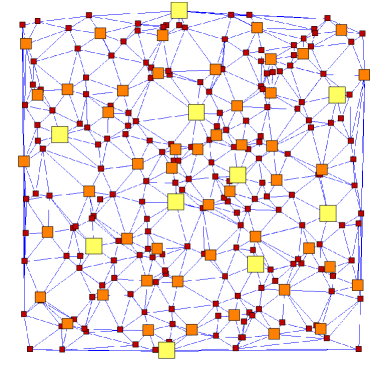
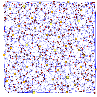
The last test we consider corresponds to a triangulation of $N$ randomly chosen points in $[0,1]\times[0,1]$. The transition probabilities in the network are then given by the inverse of the number of outgoing edges at each point, similar to the uniform network. In Figure 6, we show two examples of such networks, one with $N=256$ and one with $N=1024$ points.

(a) Random planar graph with $N=256$

(b) Random planar graph with $N=1024$

Figure 6. Delaunay-triangulations of $N$ randomly chosen points in the unit square $[0,1]\times[0,1]$.

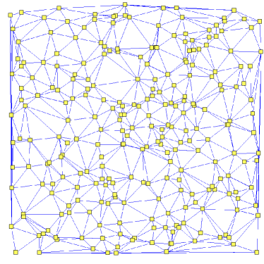
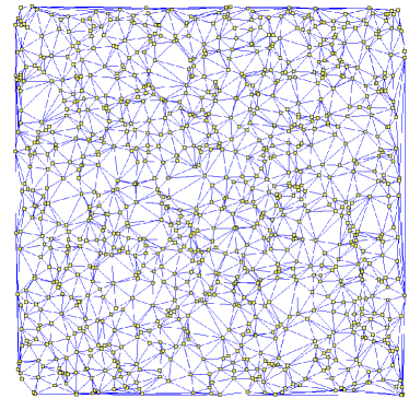
Due to the fact that the corresponding graphs of this model are planar, we call this model unstructured planar graph model. As there is no natural way to define the set of coarse variables $\mathcal{C}$ for this problem we use compatible relaxation, introduced in section 3.1 to define the splitting of variables $\Omega=\mathcal{F}\cup\mathcal{C}$. In Figure 7, a resulting coarsening is presented. The size of each individual point represents how many grids it appears on.

(a) Random planar graph with $N=256$

(b) Random planar graph with $N=1024$

Figure 7. Coarsening of Delaunay-triangulations of $N$ points randomly scattered in the unit square $[0,1]\times[0,1]$ shown in Figure 6 using compatible relaxation.

In Table 4, we report results of our overall algorithm for unstructured planar graph models for a set of varying graphs.

$N$	256	512	1024	2048
MLE	$15$	$20$	$20$	$20$
pGMRES	$8_{V}$	$10_{V}$	$10_{V}$	$11_{V}$
pArnoldi	$8_{V}$	$10_{V}$	$10_{V}$	$11_{V}$

Table 4. Multilevel ($3$ level) results for the unstructured planar graph model on a grid with $N$ points randomly scattered in the unit square. We report results to compute the steady-state vector $x$ to an accuracy of $10^{-8}$, using a $V(2,2)$-MLE cycle with $\omega$-Jacobi smoothing, $\omega=.7$. In addition we also report the number of iterations pGMRES needs to achieve the same accuracy, where we denote the initial bootstrap setup in the subscript. The sets $\mathcal{U}$ and $\mathcal{V}$ consist of $6$ initially positive random vectors and coarsest grid eigenvectors, respectively.

Even for this unstructured graph network we obtain a fast converging method with our MLE approach. The mild variation in the results when increasing the problem-size might be caused by the fact that by increasing the problem-size the nature of the problem changes in the sense that the average number of outgoing edges of grid points increases. That is, it is not necessarily clear whether two unstructured graphs of different sizes are comparable.

6. Conclusions

The proposed BootAMG Multilevel setup algorithm produces an effective multilevel eigensolver for the Markov-Chain test problems we considered. In general, we have proposed and implemented two important new ideas: First, the use of a coarse-level eigensolve and the resulting multilevel hierarchy to improve a given approximation of the state vector. Second the use of BootAMG preconditioned GMRES steps to further accelerate this eigensolver. Both ideas, separately or combined can be incorporated into any given multilevel method used for solving Markov Chain problems or other problems targeting smooth eigenvectors. The accurate representation of the near-kernel of the fine-level system on coarser levels, that results from our BootAMG setup, yields a very effective preconditioner to GMRES as well as for the Arnoldi method. An additional benefit of our proposed method over other existing multilevel method for Markov Chains is that we do not require any special processing of the coarse-level systems to ensure that stochastic properties of the fine-level system are maintained there. We mention that the developed approach is not restricted to Markov Chain problems; it can be applied to other eigenvalue problems.

References

- [1] A. Berman, R. Plemmons, Nonnegative Matrices in the Mathematical Sciences. Classics in Appl. Math. 9, SIAM, Philadelphia (1994).
- [2] A. Brandt, Multi-level Adaptive Solutions to Boundary Value Problems. Mathematics of Computation 31 (1977), pp. 333–390.
- [3] A. Brandt, General Highly Accurate Algebraic Coarsening. Electronic Transactions on Numerical Analysis 10 (2000), pp. 1–20.
- [4] A. Brandt, Multiscale Scientific Computation: Review 2001. In Barth, T.J., Chan, T.F. and Haimes, R. (eds.): Multiscale and Multiresolution Methods: Theory and Applications. Springer Verlag, Heidelberg (2001), pp. 1–96. Also available at www.wisdom.weizmann.ac.il/achi/ review00.ps.
- [5] A. Brandt, Principles of Systematic Upscaling. In: Bridging the Scales in Science and Engineering, J. Fish (Ed.), Oxford University Press (2008).
- [6] A. Brandt, J. Brannick, K. Kahl, and I. livshits, A Least Squares based Algebraic Multigrid Solver for Hermitian and Positive Definite Systems. SIAM J. Sci. Comput.., submitted.
- [7] A. Brandt and I. Livshits, A Multiscale Method for Finding Many Eigenfunctions of PDE operators. In preparation.
- [8] J. Brannick, Adaptive Agebraic Multigrid Coarsening Strategies. Ph.D. thesis (2005).
- [9] J. Brannick and R. Falgout, Compatible Relaxation and Coarsening in Algebraic Multigrid. SIAM J. Sci. Comput., to appear. Also available as LLNL technical report: LLNL-JRNL-417122
- [10] H. De Sterck, T. Manteuffel, S. McCormick, Q. Nguyen, and J. Ruge. Multilevel Adaptive Aggregation for Markov Chains with Application to Web Ranking. SIAM J. Sci. Comput. 30 (2008), pp. 2235-2262.
- [11] H. De Sterck, T. Manteuffel, S. McCormick, K. Miller, James Pearson, John Ruge, and Geoffrey Sanders. Smoothed Aggregation Multigrid. for Markov Chains. SIAM J. Sci. Comput., accepted (2009).
- [12] R. Falgout and P. Vassilevski, On Generalizing the AMG Framework. SIAM J. Numer. Anal. 42:4 (2004), pp. 1669 - 1693.
- [13] R. Falgout, P. Vassilevski, and L. Zikatanov, On Two–grid Convergence Estimates. Numerical Linear Algebra with Applications 12:5-6 (2005), pp. 471–494.
- [14] K. Hayami, M. Sugihara, A Geometric View of Krylov Subspace Methods on Singular Systems. NII Technical Report, NII-2009-007E (2009).
- [15] K. Kahl, Adaptive Algebraic Multigrid for Lattice QCD Computations. Ph.D. thesis, Department of Mathematics, Bergische Universität Wuppertal (2009).
- [16] O. Livne, Coarsening by Compatible Relaxation. Numerical Linear Algebra with Applications, 11:2-3 (2004), pp. 205–227.
- [17] I. Livshits, One-dimensional Algorithm for Finding Eigenbasis of the Schrödinger Pperator. SIAM J. Sci. Comput. 30:1 (2008), pp. 416–440.
- [18] J. Ruge, K. Stüben, Algebraic Multigrid. in Multigrid Methods, S. F. McCormick, ed., Frontiers in Applied Mathematics 3, SIAM, Philadelphia, PA (1987), pp. 73-130.
- [19] E. Seneta, Non-negative matrices and Markov chains. 2nd rev. ed., Springer Series in Statistics, NY (1981). ISBN: 978-0-387-29765-1.
- [20] H. Simon and A. Ando. Aggregation of Variables in Dynamic Systems. Econometrica 29 (1961), pp. 111- 138.
- [21] Y. Takahashi. A Lumping Method for Numerical Calculations of Sationary Distributions of Markov Chains. Research Report B-18, Department of Information Sciences, Tokyo Institute of Technology (1975).
- [22] U. Trottenberg, C. Oosterlee, and A. Schüller. Multigrid. Academic Press, San Diego (2001).
- [23] E. Virnik. An Algebraic Multigrid Preconditioner for a Class of Singular M-matrices. SIAM J. Sci. Comput. 29 (2007), pp. 1982-1991.