Universality in DAX index returns fluctuations

Abstract

In terms of the stock exchange returns, we compute the analytic expression of the probability distributions $F_{DAX,+}$ and $F_{DAX,-}$ of the normalized positive and negative DAX (Germany) index daily returns $r(t)$. Furthermore, we define the $\alpha$ re-scaled DAX daily index positive returns $r(t)^{\alpha}$ and negative returns $(-r(t))^{\alpha}$ that we call, after normalization, the $\alpha$ positive fluctuations and $\alpha$ negative fluctuations. We use the Kolmogorov-Smirnov statistical test, as a method, to find the values of $\alpha$ that optimize the data collapse of the histogram of the $\alpha$ fluctuations with the Bramwell-Holdsworth-Pinton (BHP) probability density function. The optimal parameters that we found are $\alpha^{+}=0.50$ and $\alpha^{-}=0.48$. Since the BHP probability density function appears in several other dissimilar phenomena, our results reveal universality in the stock exchange markets.

I INTRODUCTION

The modeling of the time series of stock prices is a main issue in economics and finance and it is of a vital importance in the management of large portfolios of stocks, see Gabaix (2001); Lillo (2001) and Mantegna (2001). Here we study de DAX indice. The DAX (Deutscher Aktien IndeX, formerly Deutscher Aktien-Index (German stock index)) is a blue chip stock market index that measures the development of the 30 largest and best-performing companies on the German equities market and represents around 80 $\%$ of the market capital authorized in Germany. The time series to investigate in our analysis is the DAX index from 1990 to 2009. Let $Y(t)$ be the DAX index adjusted close value at day $t$. We define the DAX index daily return on day $t$ by

$$r(t)=\frac{Y(t)-Y(t-1)}{Y(t-1)}$$

We define the $\alpha$ re-scaled DAX daily index positive returns $r(t)^{\alpha}$, for $r(t)>0$, that we call, after normalization, the $\alpha$ positive fluctuations. We define the $\alpha$ re-scaled DAX daily index negative returns $(-r(t))^{\alpha}$, for $r(t)<0$, that we call, after normalization, the $\alpha$ negative fluctuations. We analyze, separately, the $\alpha$ positive and $\alpha$ negative daily fluctuations that can have different statistical and economic natures due, for instance, to the leverage effects (see, for example, Andersen (2004); Barnhart (2009) and Pinto (2009)). Our aim is to find the values of $\alpha$ that optimize the data collapse of the histogram of the $\alpha$ positive and $\alpha$ negative fluctuations to the universal, non-parametric, Bramwell-Holdsofworth-Pinton (BHP) probability density function. To do it, we apply the Kolmogorov-Smirnov statistic test to the null hypothesis claiming that the probability distribution of the $\alpha$ fluctuations is equal to the (BHP) distribution. We observe that the $P$ values of the Kolmogorov-Smirnov test vary continuously with $\alpha$. The highest $P$ values $P^{+}=0.19...$ and $P^{-}=0.24...$ of the Kolmogorov-Smirnov test are attained for the values $\alpha^{+}=0.50...$ and $\alpha^{-}=0.48...$, respectively, for the positive and negative fluctuations. Hence, the null hypothesis is not rejected for values of $\alpha$ in small neighborhoods of $\alpha^{+}=0.50...$ and $\alpha^{-}=0.48...$. Then, we show the data collapse of the histograms of the $\alpha^{+}$ positive fluctuations and $\alpha^{-}$ negative fluctuations to the BHP pdf. Using this data collapse, we do a change of variable that allow us to compute the analytic expressions of the probability density functions $f_{DAX,+}$ and $f_{DAX,-}$ of the normalized positive and negative DAX index daily returns

$$f_{DAX,+}(x)=5.58...x^{-0.50...}f_{BHP}(22.2...x^{0.50...}-1.99...).$$

$$f_{DAX,-}(x)=4.79...x^{-0.52...}f_{BHP}(20.12....x^{0.48...}-2.01...)$$

in terms of the BHP pdf $f_{BHP}$. We exhibit the data collapse of the histogram of the positive and negative returns to our proposed theoretical pdf s $f_{DAX,+}$ and $f_{DAX,-}$. Similar results are observed for some other stock indexes, prices of stocks, exchange rates and commodity prices (see Gonçalves (2010b, c)). Since the BHP probability density function appears in several other dissimilar phenomena (see, for instance, Bramwell (2002); Dahlstedt (2001); Gonçalves (2009b, d); Pinto (2010)), our result reveals an universal feature of the stock exchange markets.

II POSITIVE DAX INDEX DAILY RETURNS

Let $T^{+}$ be the set of all days $t$ with positive returns, i.e.

$$T^{+}=\{t:r(t)>0\}.$$

Let $n^{+}=2524$ be the cardinal of the set $T^{+}$. The $\alpha$ re-scaled S&P100 daily index positive returns are the returns $r(t)^{\alpha}$ with $t\in T^{+}$. Since the total number of observed days is $n=4758$, we obtain that $n^{+}/n=0.53$. The mean $\mu^{+}_{\alpha}=0.09...$ of the $\alpha$ re-scaled DAX daily index positive returns is given by

$$\mu^{+}_{\alpha}=\frac{1}{n^{+}}\sum_{t\in T^{+}}r(t)^{\alpha}$$ (1)

The standard deviation $\sigma^{+}_{\alpha}=0.045...$ of the $\alpha$ re-scaled DAX daily index positive returns is given by

$$\sigma^{+}_{\alpha}=\sqrt{\frac{1}{n^{+}}\sum_{t\in T^{+}}{r(t)^{2\alpha}}-(\mu^{+}_{\alpha})^{2}}$$ (2)

We define the $\alpha$ positive fluctuations by

$$r^{+}_{\alpha}(t)=\frac{r(t)^{\alpha}-\mu^{+}_{\alpha}}{\sigma^{+}_{\alpha}}$$ (3)

for every $t\in T^{+}$. Hence, the $\alpha$ positive fluctuations are the normalized $\alpha$ re-scaled $DAX$ daily index positive returns. Let $L^{+}_{\alpha}=-1.90...$ be the smallest $\alpha$ positive fluctuation, i.e.

$$L^{+}_{\alpha}=\min_{t\in T^{+}}\{r^{+}_{\alpha}(t)\}.$$

Let $R^{+}_{\alpha}=5.51...$ be the largest $\alpha$ positive fluctuation, i.e.

$$R^{+}_{\alpha}=\max_{t\in T^{+}}\{r^{+}_{\alpha}(t)\}.$$

We denote by $F_{\alpha,+}$ the probability distribution of the $\alpha$ positive fluctuations. Let the truncated BHP probability distribution $F_{BHP,\alpha,+}$ be given by

$$F_{BHP,\alpha,+}(x)=\frac{F_{BHP}(x)}{F_{BHP}(R^{+}_{\alpha})-F_{BHP}(L^{+}_{\alpha})}$$

where $F_{BHP}$ is the BHP probability distribution.

We apply the Kolmogorov-Smirnov statistic test to the null hypothesis claiming that the probability distributions $F_{\alpha,+}$ and $F_{BHP,\alpha,+}$ are equal. The Kolmogorov-Smirnov $P$ value $P_{\alpha,+}$ is plotted in Figure 1. Hence, we observe that $\alpha^{+}=0.50...$ is the point where the $P$ value $P_{\alpha,+}=0.19...$ attains its maximum.

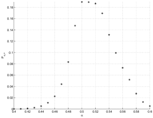
Figure 1: The Kolmogorov-Smirnov $P$ value $P_{\alpha,+}$ for values of $\alpha$ in the range $[0.4,0.6]$.

It is well-known that the Kolmogorov-Smirnov $P$ value $P_{\alpha,+}$ decreases with the distance $\left\|F_{\alpha,+}-F_{BHP,\alpha,+}\right\|$ between $F_{\alpha,+}$ and $F_{BHP,\alpha,+}$.

In Figure 2, we plot $D_{\alpha^{+},+}(x)=\left|F_{\alpha^{+},+}(x)-F_{BHP,\alpha^{+},+}(x)\right|$ and we observe that $D_{\alpha^{+},+}(x)$ attains its highest values for the $\alpha^{+}$ positive fluctuations below or close to the mean of the probability distribution.

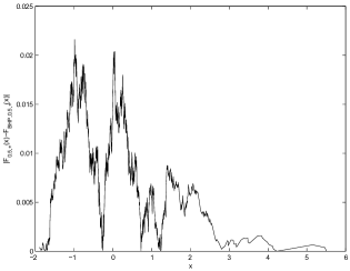
Figure 2: The map $D_{0.50,+}(x)=|F_{0.50,+}(x)-F_{BHP,0.50,+}(x)|$.

In Figures 3 and 4, we show the data collapse of the histogram $f_{\alpha^{+},+}$ of the $\alpha^{+}$ positive fluctuations to the truncated BHP pdf $f_{BHP,\alpha^{+},+}$.

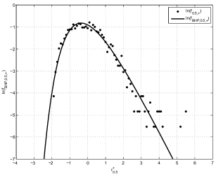
Figure 3: The histogram of the $\alpha^{+}$ positive fluctuations with the truncated BHP pdf $f_{BHP,0.50,+}$ on top, in the semi-log scale.

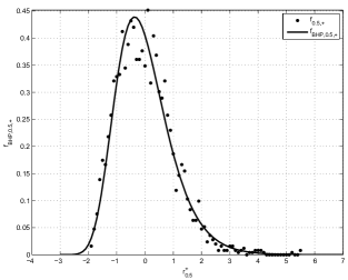
Figure 4: The histogram of the $\alpha^{+}$ positive fluctuations with the truncated BHP pdf $f_{BHP,0.50,+}$ on top.

Assume that the probability distribution of the $\alpha^{+}$ positive fluctuations $r^{+}_{\alpha^{+}}(t)$ is given by $F_{BHP,\alpha^{+},+}$, see Gonçalves (2009a). The pdf $f_{DAX,+}$ of the DAX daily index positive returns $r(t)$ is given by

$$f_{DAX,+}(x)=\frac{\alpha^{+}x^{\alpha^{+}-1}f_{BHP}\left(\left(x^{\alpha^{+}}-\mu^{+}_{\alpha^{+}}\right)/\sigma^{+}_{\alpha^{+}}\right)}{\sigma^{+}_{\alpha^{+}}\left(F_{BHP}\left(R^{+}_{\alpha^{+}}\right)-F_{BHP}\left(L^{+}_{\alpha^{+}}\right)\right)}.$$

Hence, taking $\alpha^{+}=0.50...$, we get

$$f_{DAX,+}(x)=5.58...x^{-0.50...}f_{BHP}(22.2...x^{0.50...}-1.99...).$$

In Figures 5 and 6 , we show the data collapse of the histogram $f_{1,+}$ of the positive returns to our proposed theoretical pdf $f_{DAX,+}$.

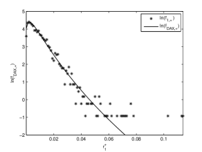
Figure 5: The histogram of the fluctuations of the positive returns with the pdf $f_{DAX,+}$ on top, in the semi-log scale.

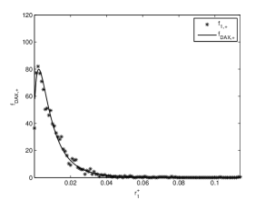
Figure 6: The histogram of the fluctuations of the positive returns with the pdf $f_{DAX,+}$ on top.

III NEGATIVE DAX INDEX DAILY RETURNS

Let $T^{-}$ be the set of all days $t$ with negative returns, i.e.

$$T^{-}=\{t:r(t)<0\}.$$

Let $n^{-}=2221$ be the cardinal of the set $T^{-}$. Since the total number of observed days is $n=4758$, we obtain that $n^{-}/n=0.47$. The $\alpha$ re-scaled DAX daily index negative returns are the returns $(-r(t))^{\alpha}$ with $t\in T^{-}$. We note that $-r(t)$ is positive. The mean $\mu^{-}_{\alpha}=0.10...$ of the $\alpha$ re-scaled DAX daily index negative returns is given by

$$\mu^{-}_{\alpha}=\frac{1}{n^{-}}\sum_{t\in T^{-}}(-r(t))^{\alpha}$$ (4)

The standard deviation $\sigma^{-}_{\alpha}=0.050...$ of the $\alpha$ re-scaled DAX daily index negative returns is given by

$$\sigma^{-}_{\alpha}=\sqrt{\frac{1}{n^{-}}\sum_{t\in T^{-}}{(-r(t))^{2\alpha}}-(\mu^{-}_{\alpha})^{2}}$$ (5)

We define the $\alpha$ negative fluctuations by

$$r^{-}_{\alpha}(t)=\frac{(-r(t))^{\alpha}-\mu^{-}_{\alpha}}{\sigma^{-}_{\alpha}}$$ (6)

for every $t\in T^{-}$. Hence, the $\alpha$ negative fluctuations are the normalized $\alpha$ re-scaled $DAX$ daily index negative returns. Let $L^{-}_{\alpha}=-1.94...$ be the smallest $\alpha$ negative fluctuation, i.e.

$$L^{-}_{\alpha}=\min_{t\in T^{-}}\{r^{-}_{\alpha}(t)\}.$$

Let $R^{-}_{\alpha}=4.45...$ be the largest $\alpha$ negative fluctuation, i.e.

$$R^{-}_{\alpha}=\max_{t\in T^{-}}\{r^{-}_{\alpha}(t)\}.$$

We denote by $F_{\alpha,-}$ the probability distribution of the $\alpha$ negative fluctuations. Let the truncated BHP probability distribution $F_{BHP,\alpha,-}$ be given by

$$F_{BHP,\alpha,-}(x)=\frac{F_{BHP}(x)}{F_{BHP}(R^{-}_{\alpha})-F_{BHP}(L^{-}_{\alpha})}$$

where $F_{BHP}$ is the BHP probability distribution.

We apply the Kolmogorov-Smirnov statistic test to the null hypothesis claiming that the probability distributions $F_{\alpha,-}$ and $F_{BHP,\alpha,-}$ are equal.

The Kolmogorov-Smirnov $P$ value $P_{\alpha,-}$ is plotted in Figure 7. Hence, we observe that $\alpha^{-}=0.48...$ is the point where the $P$ value $P_{\alpha^{-}}=0.24...$ attains its maximum.

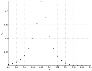
Figure 7: The Kolmogorov-Smirnov $P$ value $P_{\alpha,-}$ for values of $\alpha$ in the range $[0.4,0.6]$.

The Kolmogorov-Smirnov $P$ value $P_{\alpha,-}$ decreases with the distance $\left\|F_{\alpha,-}-F_{BHP,\alpha,-}\right\|$ between $F_{\alpha,-}$ and $F_{BHP,\alpha,-}$.

In Figure 8, we plot $D_{\alpha^{-},-}(x)=\left|F_{\alpha^{-},-}(x)-F_{BHP,\alpha^{-},-}(x)\right|$ and we observe that $D_{\alpha^{-},-}(x)$ attains its highest values for the $\alpha^{-}$ negative fluctuations above the mean of the probability distribution.

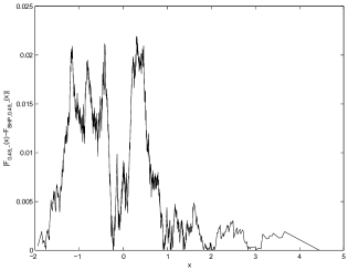
Figure 8: The map $D_{0.48,-}(x)=|F_{0.48,-}(x)-F_{BHP,0.48,-}(x)|$.

In Figures 9 and 10, we show the data collapse of the histogram $f_{\alpha^{-},-}$ of the $\alpha^{-}$ negative fluctuations to the truncated BHP pdf $f_{BHP,\alpha^{-},-}$.

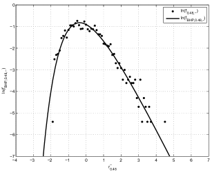
Figure 9: The histogram of the $\alpha^{-}$ negative fluctuations with the truncated BHP pdf $f_{BHP,0.48,-}$ on top, in the semi-log scale.

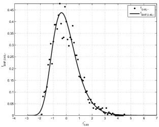
Figure 10: The histogram of the $\alpha^{-}$ negative fluctuations with the truncated BHP pdf $f_{BHP,0.48,-}$ on top.

Assume that the probability distribution of the $\alpha^{-}$ negative fluctuations $r^{-}_{\alpha^{-}}(t)$ is given by $F_{BHP,\alpha^{-},-}$, see Gonçalves (2009a). The pdf $f_{DAX,-}$ of the DAX daily index (symmetric) negative returns $-r(t)$, with $T\in T^{-}$, is given by

$$f_{DAX,-}(x)=\frac{\alpha^{-}x^{\alpha^{-}1}f_{BHP}\left(\left(x^{\alpha^{-}}-\mu^{-}_{\alpha^{-}}\right)/\sigma^{-}_{\alpha^{-}}\right)}{\sigma^{-}_{\alpha^{-}}\left(F_{BHP}\left(R^{-}_{\alpha^{-}}\right)-F_{BHP}\left(L^{-}_{\alpha^{-}}\right)\right)}.$$

Hence, taking $\alpha^{-}=0.49...$, we get

$$f_{DAX,-}(x)=4.79...x^{-0.52...}f_{BHP}(20.12....x^{0.48...}-2.01...)$$

In Figures 11 and 12, we show the data collapse of the histogram $f_{1,-}$ of the negative returns to our proposed theoretical pdf $f_{DAX,-}$.

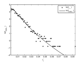
Figure 11: The histogram of the negative returns with the pdf $f_{DAX,-}$ on top, in the semi-log scale.

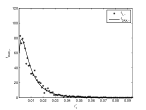
Figure 12: The histogram of the negative returns with the pdf $f_{DAX,-}$ on top.

IV CONCLUSIONS

We used the Kolmogorov-Smirnov statistical test to compare the histogram of the $\alpha$ positive fluctuations and $\alpha$ negative fluctuations with the universal, non-parametric, Bramwell-Holdsworth-Pinton (BHP) probability distribution. We found that the parameters $\alpha^{+}=0.50...$ and $\alpha^{-}=0.48...$ for the positive and negative fluctuations, respectively, optimize the $P$ value of the Kolmogorov-Smirnov test. We obtained that the respective $P$ values of the Kolmogorov-Smirnov statistical test are $P^{+}=0.19...$ and $P^{-}=0.23...$. Hence, the null hypothesis was not rejected. The fact that $\alpha^{+}$ is different from $\alpha^{-}$ can be do to leverage effects. We presented the data collapse of the corresponding fluctuations histograms to the BHP pdf. Furthermore, we computed the analytic expression of the probability distributions $F_{DAX,+}$ and $F_{DAX,-}$ of the normalized DAX index daily positive and negative returns in terms of the BHP pdf. We showed the data collapse of the histogram of the positive and negative returns to our proposed theoretical pdfs $f_{DAX,+}$ and $f_{DAX,-}$. The results obtained in daily returns also apply to other periodicities, such as weekly and monthly returns as well as intraday values.

In Gonçalves (2010b, 2009a); Peixoto (2001), it is found the data collapses of the histograms of some other stock indexes, prices of stocks, exchange rates and commodity prices to the BHP pdf and in Gonçalves (2010a) for energy sources.

Bramwell, Holdsworth and Pinton Bramwell (1998) found the probability distribution of the fluctuations of the total magnetization, in the strong coupling (low temperature) regime, for a two-dimensional spin model (2dXY) using the spin wave approximation. From a statistical physics point of view, one can think that the stock prices form a non-equilibrium system Chowdhury (1999); Gopikrishnan (1998); Lillo (2001); Plerou (1999). Hence, the results presented here lead to a construction of a new qualitative and quantitative econophysics model for the stock market based in the two-dimensional spin model (2dXY) at criticality (see Gonçalves (2010c)).

Appendix A BRAMWELL-HOLDSWORTH-PINTON PROBABILITY DISTRIBUTION

The universal nonparametric BHP pdf was discovered by Bramwell, Holdsworth and Pinton Bramwell (1998). The BHP probability density function (pdf) is given by

$$f_{BHP}(\mu)=\int_{-\infty}^{\infty}\frac{dx}{2\pi}\sqrt{\frac{1}{2N^{2}}\sum_{k=1}^{N-1}\frac{1}{\lambda_{k}^{2}}}e^{ix\mu\sqrt{\frac{1}{2N^{2}}\sum_{k=1}^{N-1}\frac{1}{\lambda_{k}^{2}}}}$$

$$.e^{-\sum_{k=1}^{N-1}\left[\frac{ix}{2N}\frac{1}{\lambda_{k}}-\frac{i}{2}\mbox{arctan}\left(\frac{x}{N\lambda_{k}}\right)\right]}.e^{-\sum_{k=1}^{N-1}\left[\frac{1}{4}\mbox{ln}{\left(1+\frac{x^{2}}{N^{2}\lambda_{k}^{2}}\right)}\right]}$$

(7)

where the $\{\lambda_{k}\}_{k=1}^{L}$ are the eigenvalues, as determined in Bramwell (2001), of the adjacency matrix. It follows, from the formula of the BHP pdf, that the asymptotic values for large deviations, below and above the mean, are exponential and double exponential, respectively (in this article, we use the approximation of the BHP pdf obtained by taking $L=10$ and $N=L^{2}$ in equation (7)). As we can see, the BHP distribution does not have any parameter (except the mean that is normalize to 0 and the standard deviation that is normalized to 1) and it is universal, in the sense that appears in several physical phenomena. For instance, the universal nonparametric BHP distribution is a good model to explain the fluctuations of order parameters in theoretical examples such as, models of self-organized criticality, equilibrium critical behavior, percolation phenomena (see Bramwell (1998)), the Sneppen model (see Bramwell (1998) and Dahlstedt (2001)), and auto-ignition fire models (see Sinha-Ray (2001)). The universal nonparametric BHP distribution is, also, an explanatory model for fluctuations of several phenomenon such as, width power in steady state systems (see Bramwell (1998)), fluctuations in river heights and flow (see Bramwell (2001); Gonçalves (2009b, c)), for the plasma density fluctuations and electrostatic turbulent fluxes measured at the scrape-off layer of the Alcator C-mod Tokamaks (see Van Milligen (2005)) and for Wolf’s sunspot numbers fluctuations (see Gonçalves (2009d)).

References

- Andersen (2004) Andersen, T.G., Bollerslev, T., Frederiksen, P. and Nielse, M., 2004, Continuos-Time Models, Realized Volatilities and Testable Distributional Implications for Daily Stock Returns Preprint.
- Barnhart (2009) Barnhart, S. W. & Giannetti, A., 2009, Negative earnings, positive earnings and stock return predictability: An empirical examination of market timing Journal of Empirical Finance 16 70-86.
- Bramwell (1998) Bramwell, S.T., Holdsworth, P.C.W., & Pinton, J.F., 1998,Nature, 396 552-554.
- Bramwell (2002) Bramwell, S.T., Fennell, T., Holdsworth, P.C.W.,& Portelli, B., 2002, Universal Fluctuations of the Danube Water Level: a Link with Turbulence, Criticality and Company Growth, Europhysics Letters 57 310.
- Bramwell (2001) Bramwell, S.T., Fortin, J.Y., Holdsworth, P.C.W., Peysson, S., Pinton, J.F., Portelli, B. & Sellitto, M., 2001, Magnetic Fluctuations in the classical XY model: the origin of an exponential tail in a complex system, Phys. Rev E 63 041106.
- Chowdhury (1999) Chowdhury, D. and Stauffer, D., 1991, A generalized spin model of financial markets Eur. Phys. J. B8 477-482.
- Dahlstedt (2001) Dahlstedt, K., & Jensen, H.J., 2001, Universal fluctuations and extreme-value statistics, J. Phys. A: Math. Gen. 34 11193-11200.
- Peixoto (2001) Dynamics, Games and Science., 2010, Eds: M. Peixoto, A. A. Pinto and D. A. Rand. Proceedings in Mathematics series, Springer-Verlag.
- Gabaix (2001) Gabaix, X., Parameswaran, G., Plerou, V. & Stanley, E., 2003, A theory of power-law distributions in financial markets Nature 423 267-270.
- Gonçalves (2009a) Gonçalves, R., Ferreira, H. and Pinto, A. A., 2009a, Universality in the Stock Exchange Market Journal of Difference Equations and Applications (accepted).
- Gonçalves (2010a) Gonçalves, R., Ferreira, H. and Pinto, A. A., 2010a, Universality in energy sources, IAEE (International Association for Energy economics) International Conference (accepted).
- Gonçalves (2010b) Gonçalves, R., Ferreira, H. and Pinto, A. A., 2010b, Universal fluctuations of the Dow Jones (submitted).
- Gonçalves (2010c) Gonçalves, R., Ferreira, H. and Pinto, A. A., 2010c, A qualitative and quantitative Econophysics stock market model (submitted).
- Gonçalves (2009b) Gonçalves, R., Ferreira, H., Pinto, A. A. and Stollenwerk, N., 2009b, Universality in nonlinear prediction of complex systems. Special issue in honor of Saber Elaydi. Journal of Difference Equations and Applications 15, Issue 11 & 12, 1067-1076.
- Gonçalves (2009c) Gonçalves, R., and Pinto, A. A., 2009c, Negro and Danube are mirror rivers. Special issue Dynamics & Applications in honor of Mauricio Peixoto and David Rand. Journal of Difference Equations and Applications.
- Gonçalves (2009d) Gonçalves, R. Pinto, A. A., Stollenwerk, N., 2009d, Cycles and universality in sunspot numbers fluctuations The Astrophysical Journal 691 1583-1586.
- Gopikrishnan (1998) Gopikrishnan, P., Meyer, M., Amaral, L. & Stanley, H., 1998, Inverse cubic law for the distribution of stock price variation The European Physical Journal B 3 139-140.
- Lillo (2001) Lillo, F. and Mantegna, R., 2001, Ensemble Properties of securities traded in the Nasdaq market Physica A 299 161-167 (2001).
- Mantegna (2001) Mantegna, R. & Stanley, E., 2001, Scaling behaviour in the dynamics of a economic index Nature 376 46-49.
- Pinto (2010) Pinto, A. A., 2010, Game theory and Duopoly Models Interdisciplinary Applied Mathematics, Springer-Verlag.
- Pinto (2009) Pinto, A. A., Rand, D. A. and Ferreira, F., 2009, Fine Structures of Hyperbolic Diffeomorphisms. Springer-Verlag Monograph.
- Plerou (1999) Plerou, V., Amaral, L., Gopikrishnan, P., Meyer, M. & Stanley, E., 1999, Universal and Nonuniversal Properties of Cross Correlations in Financial Time Series Physical Review Letters 83 7 1471-1474.
- Sinha-Ray (2001) Sinha-Ray, P., Borda de Água, L. & Jensen, H.J., 2001, Threshold dynamics, multifractality and universal fluctuations in the SOC forest fire: facets of an auto-ignition model Physica D 157, 186–196.
- Van Milligen (2005) Van Milligen, B. Ph., Sánchez, R., Carreras, B. A., Lynch, V. E., LaBombard, B., Pedrosa, M. A., Hidalgo, C., Gonçalves, B. & Balbín, R., 2005, Physics of plasmas 12 05207.