Distribution of chirality in the quantum walk: Markov process and entanglement

Abstract

The asymptotic behavior of the quantum walk on the line is investigated focusing on the probability distribution of chirality independently of position. It is shown analytically that this distribution has a long-time limit that is stationary and depends on the initial conditions. This result is unexpected in the context of the unitary evolution of the quantum walk, as it is usually linked to a Markovian process. The asymptotic value of the entanglement between the coin and the position is determined by the chirality distribution. For given asymptotic values of both the entanglement and the chirality distribution it is possible to find the corresponding initial conditions within a particular class of spatially extended Gaussian distributions.

I Introduction

The quantum walk (QW) on the line QW is a natural generalization of the classical random walk in the frame of quantum computation and quantum information processing and it is receiving permanent attentionchilds ; Linden ; Alejo3 . It has the property to spread over the line linearly in time as characterized by the standard deviation $\sigma(t)\sim t$, while its classical analog spreads out as $\sigma(t)\sim t^{1/2}$. This property, as well as quantum parallelism and quantum entanglement, could be used to increase the efficiency of quantum algorithms. As an example the QW has been used as the basis for optimal quantum search algorithms Shenvi ; Childs et on several topologies. On the other hand, some experimental implementations of the QW have been reported Exp , and others have been proposed by a number of authors ProExp .

The concept of entanglement is an important element in the development of quantum communication, quantum cryptography and quantum computation. In this context, several authors have studied the QW subjected to different types of coin operators and/or sources of decoherence to analyze the long-time entanglement between the coin and the position and its relation with the initial conditions. Carneiro et al. Carneiro investigate entanglement between the coin and the position calculating the entropy of the reduced density matrix of the coin. The relation between asymptotic entanglement and nonlocal initial conditions (in the one and two dimensional QW) is treated in abal ; Annabestani ; Omar ; Pathak ; Petulante ; Venegas . Ref. Endrejat ; Ellinas1 ; Ellinas2 analyze the effect of entanglement on the initial coin state, which is measured by the mean value of the walk, and the relation between the entanglement and the symmetry of the probability distribution. In Ref. Maloyer the relation between entanglement and decoherence is studied numerically. Refs. Venegas1 ; Chandrashekar propose to use the QW as a tool for quantum algorithm development and as entanglement generator, potentially useful to test quantum hardware.

In the previous works Carneiro ; abal ; Annabestani ; Omar ; Pathak ; Petulante ; Venegas ; Endrejat ; Ellinas1 ; Ellinas2 ; Maloyer ; Venegas1 ; Chandrashekar the QW evolution was studied using the amplitude of probability to evaluate the dynamics. In this work we introduce a new probability distribution, the global chirality distribution (GCD) that is the distribution of chirality independently of the walker’s position. We show that the GCD has an asymptotic limit and we connect this limit with the entropy of entanglement between the coin and the position. The asymptotic behavior of GCD is an unexpected result because, due to the unitary evolution, the QW does not converge to any stationary state as would be the case e.g. of a Markov chain. In order to show these results, we rewrite the QW evolution equation as the sum of two different terms, one responsible for the classical diffusion and the other for the quantum coherence Alejo1 . As we shall see, the first term above obeys a master equation as is typical of Markovian processes, while the second term includes the interference needed to preserve the unitary character of the quantum evolution. This approach provides a more intuitive framework which proves useful for analyzing the behavior of quantum systems with decoherence. It allows to study the quantum evolution together with the associated classical Markovian process at all times, and in particular the asymptotic behavior of the GCD.

The paper is organized as follows. In the next section we develop the standard QW model, in the third section we build the master equation for the GCD, in the fourth section we present the asymptotic solution for the QW, in the fifth section the entropy of entanglement is connected with the GCD, and in the last section we draw the conclusions.

II The standard QW

The QW on the line, corresponds to a one-dimensional evolution of a quantum system in a direction which depends on an additional degree of freedom, the chirality, with two possible states: “left” $|L\rangle$ or “right” $|R\rangle$. The global Hilbert space of the system is the tensor product $H_{s}\otimes H_{c}$ where $H_{s}$ is the Hilbert space associated to the motion on the line and $H_{c}$ is the chirality Hilbert space. Let us call $T_{-}$ ($T_{+}$) the operators in $H_{s}$ that move the walker one site to the left (right), and $|L\rangle\langle L|$ and $|R\rangle\langle R|$ the chirality projector operators in $H_{c}$. We consider the unitary transformations

$$U(\theta)=\left\{T_{-}\otimes|L\rangle\langle L|+T_{+}\otimes|R\rangle\langle R|\right\}\circ\left\{I\otimes K(\theta)\right\},$$ (1)

where $K(\theta)=\sigma_{z}\cos\theta+i\sigma_{x}\sin\theta$, $I$ is the identity operator in $H_{s}$, and $\sigma_{z}$ and $\sigma_{x}$ are Pauli matrices acting in $H_{c}$. The unitary operator $U(\theta)$ evolves the state in one time step as

$$|\Psi(t+1)\rangle=U(\theta)|\Psi(t)\rangle.$$ (2)

The wave vector can be expressed as the spinor

$$|\Psi(t)\rangle=\sum\limits_{k=-\infty}^{\infty}\left[\begin{array}[]{c}a_{k}(t)\\ b_{k}(t)\end{array}\right]|k\rangle,$$ (3)

where the upper (lower) component is associated to the left (right) chirality. Substituting Eq. (3) and Eq. (1) into Eq. (2) and projecting over the position vector $|k\rangle$ the unitary evolution is written as the map

$$a_{k}(t+1) =a_{k+1}(t)\,\cos\theta\,+b_{k+1}(t)\,\sin\theta,\,$$

$$b_{k}(t+1) =a_{k-1}(t)\,\sin\theta\,-b_{k-1}(t)\,\cos\theta.$$ (4)

III unitary evolution and master equation for the chirality

In references Alejo1 ; Alejo2 , it is shown how a unitary quantum mechanical evolution can be separated into Markovian and interference terms. Here we use this method to recognize a master equation in chirality starting from the original map Eq. (4). First we define the left and right distributions of position as $P_{kL}(t)=\left|a_{k}(t)\right|^{2}$ and $P_{kR}(t)~{}\equiv~{}\left|b_{k}(t)\right|^{2}$ respectively. Combining the two components of the Eq. (4) and after some simple algebra we obtain

$$P_{k,L}(t+1) =P_{k+1,L}(t)\,\cos^{2}\theta+P_{k+1,R}(t)\,\sin^{2}\theta$$

$$+\beta_{k+1}(t)\,\sin 2\theta,$$

$$P_{k,R}(t+1) =P_{k-1,L}(t)\,\sin^{2}\theta+P_{k-1,R}(t)\,\cos^{2}\theta$$

$$-\beta_{k-1}(t)\,\sin 2\theta\,,$$ (5)

where $\beta_{k}\equiv\mathrm{Re}\left[a_{k}(t)b_{k}^{\ast}(t)\right]$ is an interference term, with $\mathrm{Re}(z)$ indicating the real part of $z$. Of course the probability distribution for the position is $P_{k}(t)=P_{kL}(t)+P_{kR}(t)$. We define the global left and right chirality probabilities as

$$P_{L}(t)\equiv\sum_{k=-\infty}^{\infty}P_{kL}(t)=\sum_{k=-\infty}^{\infty}\left|a_{k}(t)\right|^{2},\,$$

$$P_{R}(t)\equiv\sum_{k=-\infty}^{\infty}P_{kR}(t)=\sum_{k=-\infty}^{\infty}\left|b_{k}(t)\right|^{2},$$ (6)

with $P_{R}(t)+P_{L}(t)=1$ and the global chirality distribution (GCD) is defined as the distribution formed by the couple $\left[\begin{array}[]{c}P_{L}(t)\\ P_{R}(t)\end{array}\right]$.

Using the definition Eq. (6) in Eq. (5) we have

$${\left[\begin{array}[]{c}P_{L}(t+1)\\ P_{R}(t+1)\end{array}\right]} ={\left(\begin{array}[]{cc}\cos^{2}\theta&\sin^{2}\theta\\ \sin^{2}\theta&\cos^{2}\theta\end{array}\right)}\left[\begin{array}[]{c}P_{L}(t)\\ P_{R}(t)\end{array}\right]$$ (13)

$$+\mathrm{Re}\left[Q(t)\right]\sin{2}\theta\left[\begin{array}[]{c}1\\ -1\end{array}\right],$$ (16)

where

$$Q(t)\equiv\sum_{k=-\infty}^{\infty}a_{k}(t)b_{k}^{\ast}(t).$$ (17)

In Eq. (16) the two dimensional matrix can be interpreted as a transition probability matrix for a classical two dimensional random walk as it satisfies the necessary requirements, namely, all its elements are positive and the sum over the elements of any column or row is equal to one. On the other hand, it is clear that $Q(t)$ accounts for the interferences. When $Q(t)$ vanishes the behavior of the GCD can be described as a classical Markovian process. However $Q(t)=0$ does not necessarily imply the loss of unitary evolution; such a loss requires the vanishing of all the $\beta_{k}(t)$ (see Eq (5)). As shown in Ref. Alejo4 the primary effect of decoherence is to make the interference terms $\beta_{k}(t)$ negligible; in this case Eq. (5) becomes a true master equation. On the other hand, when $Q(t)$ is time independent, that is $Q(t)=Q=constant$, then Eq. (16) is solved using the methods developed in Cox ; its solution as a function of the initial GCD is

$${\left[\begin{array}[]{c}P_{L}(t)\\ P_{R}(t)\end{array}\right]} = \frac{1}{2}{\left(\begin{array}[]{cc}1+\cos^{t}2\theta&1-\cos^{t}2\theta\\ 1-\cos^{t}2\theta&1+\cos^{t}2\theta\end{array}\right)}\left[\begin{array}[]{c}P_{L}(0)\\ P_{R}(0)\end{array}\right]$$ (27)

$$+\mathrm{Re}\left[Q\right]\frac{1-\cos^{t}2\theta}{\tan\theta}\left[\begin{array}[]{c}1\\ -1\end{array}\right].$$

Taking the limit $t\rightarrow\infty$ in Eq. (27) it is possible to obtain the asymptotic value of the GCD as a function of its initial value and $Q$.

In the generic case $Q(t)$ is a time depend function but in this system (as will be seen in the next section) $Q(t)$, $P_{L}(t)$ and $P_{R}(t)$ have long-time limiting values which are determined by the initial conditions of Eq. (4). Therefore we can solve Eq. (16) in this limit, defining

$$\Pi_{L}\equiv P_{L}(t\rightarrow\infty),\,$$

$$\Pi_{R}\equiv P_{R}(t\rightarrow\infty),\,$$

$$Q_{0}\equiv Q(t\rightarrow\infty),\,$$ (28)

and substituting these asymptotic values in Eq. (16), to obtain the stationary solution for the GCD

$${\left[\begin{array}[]{c}\Pi_{L}\\ \Pi_{R}\end{array}\right]}=\frac{1}{2}\left[\begin{array}[]{c}1+2\mathrm{Re}(Q_{0})/\tan\theta\\ 1-2\mathrm{Re}(Q_{0})/\tan\theta\end{array}\right].$$ (29)

This interesting result for the QW shows that the long-time probability to find the system with left or right chirality has a limit.

In the next section we show that it is possible to have $Q_{0}=0$ choosing adequately the initial conditions. In this case, Eq.(16) approaches a Markov chain Cox with two states and the dynamics of the GDC turns into an example of dependent Bernoulli trials in which the probabilities of success or failure et each trial depend on the outcome of the previous trial. Now the only asymptotic solution is $\Pi_{L}=\Pi_{R}=1/2$ (see Eq.(29)).

If we look back at Eq.(2) in connection with Eq.(29) a paradoxical situation arises. The dynamical evolution of the QW is unitary but the evolution of its GCD has an asymptotic value characteristic of a diffusive behavior. This situation is further surprising if we compare our case with the case of the QW on finite graphs Aharonov where it is shown that there is no converge to any stationary distribution.

IV Asymptotic solution for the QW

In previous works Alejo2 ; Alejo3 an alternative analytical approach was presented to obtain the asymptotic behavior of the QW on the line. The discrete map was substituted by two continuous differential equations for $a_{k}(t)$ and $b_{k}(t)$ starting from a characteristic time $t_{0}>>1$. The initial conditions for these equations are not necessarily the same as those used in the discrete map Eqs. (4), because the approximation of a finite difference by a derivative does not hold for small times. However these initial conditions must assure the same asymptotic behavior than that of the discrete map.

The asymptotic solutions of Eqs. (4) given by the differential equations are

$$a_{k}(t)\simeq\sum\limits_{l=-\infty}^{\infty}\left(-1\right)^{k-l}a_{l}^{0}\text{ }\,J_{k-l}(t\,\cos\theta),\,$$

$$b_{k}(t)\simeq\sum\limits_{l=-\infty}^{\infty}\left(-1\right)^{k-l}b_{l}^{0}\text{ }\,J_{k-l}(t\,\cos\theta),$$ (30)

where $J_{l}$ is the $l$th order cylindrical Bessel function and $a_{k}^{0}$ and $b_{k}^{0}$ are initial amplitudes for the differential equations. To secure that the behavior of the discrete map and the differential equations are the same in the asymptotic regime we should choose ${a_{k}^{0}}$ and ${b_{k}^{0}}$ to be smoothly extended in space.

Replacing Eq. (30) in Eqs. (6, 17) and noting that the Bessel functions satisfy $\sum_{j=-\infty}^{\infty}J_{j}(t)J_{j-k}(t)=\delta_{k0}$ we have

$$Q(t)=\sum_{k=-\infty}^{\infty}a_{k}^{0}b_{k}^{0\ast}=Q_{0},$$ (31)

$$P_{L}(t)=\sum_{j=-\infty}^{\infty}\left|a_{k}^{0}\right|^{2}=\Pi_{L},$$ (32)

$$P_{R}(t)=\sum_{k=-\infty}^{\infty}\left|b_{k}^{0}\right|^{2}=\Pi_{R}.$$ (33)

The time independence of $Q(t)$, $P_{L}(t)$ and $P_{R}(t)$ is a consequence of the asymptotic approach given by Eq. (30) and evidently their values are $Q_{0}$, $\Pi_{L}$ and $\Pi_{R}$ respectively. When $Q(t)$, $P_{L}(t)$ and $P_{R}(t)$ are calculated with the map Eq. (4), they have a transient time dependence (for $t<t_{0}$) after which they attain their asymptotic values $Q_{0}$, $\Pi_{L}$ and $\Pi_{R}$, as shown in Alejo2 .

We propose for the initial conditions $a_{k}^{0}$ and $b_{k}^{0}$ the following extended Gaussian distributions Eugenio

$$a_{k}^{0}\equiv\left\{\frac{1}{\sigma_{0}\sqrt{2\pi}}\exp\left[-\frac{(k-k_{0})^{2}}{2\sigma_{0}^{2}}\right]\right\}^{\frac{1}{2}}\cos\alpha\text{,}$$ (34)

$$b_{k}^{0}\equiv a_{k}^{0}\,\tan\alpha\,\exp(i\delta)\text{,}$$ (35)

where $\sigma_{0}$ is the initial standard deviation, $k_{0}$ is the central position of the Gaussian distribution, $\alpha$ is a parameter that determines the initial proportion of the left and right chiralities and $\delta$ is a phase to be determined bellow as a function of $\alpha$ and $\theta$.

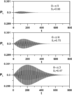
Figure 1: The global left probability $P_{L}(t)$ as a function of the dimensionless time $t$ calculated with the map Eq. (4). The initial conditions are given by Eqs. (34, 35). It is shown for three values of $\theta$, ${\sigma_{0}=100}$, $k_{0}=0$ and $\cos^{2}\alpha=0.3$. The approximate values of $t_{0}$ are, from top to bottom, $300,500,700$. The asymptotic values for the dimensionless entropy $S_{0}$ are also presented.

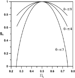
Figure 2: The dimensionless entropy of entanglement $S_{0}$ as a function of the asymptotic global left probability $\Pi_{L}$ for three different values of $\theta$.

Now we evaluate $Q_{0}$, $\Pi_{L}$ and $\Pi_{R}$ using the initial conditions Eqs. (34, 35) in Eqs. (31, 32, 33) and noting that $\sum_{k=-\infty}^{\infty}\exp\left[-\frac{k^{2}}{2\sigma_{0}^{2}}\right]\cong\sqrt{2\pi}\sigma_{0}$, for $\sigma_{0}\gg 1$

$$Q_{0}=\frac{1}{2}\sin 2\alpha\,\cos\delta\,,$$ (36)

$$\Pi_{L}=\cos^{2}\alpha\,,$$ (37)

$$\Pi_{R}=\sin^{2}\alpha\,.$$ (38)

On the other hand, from Eq. (29) we see that $Q_{0}$ and $\Pi_{L}$ are not independent, then substituting Eqs. (36, 37, 38) into Eq. (29) we have

$$\cos\delta=\frac{\tan\theta}{\tan 2\alpha}\,.$$ (39)

Then, we rewrite Eq. (36) as a function of the two independent parameters of the model $\theta$ and $\alpha$

$$Q_{0}=\frac{1}{2}\cos 2\alpha\,\tan\theta\,,$$ (40)

note that $Q_{0}$ vanishes for $\alpha=\pi/4$.

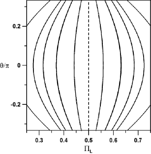
Figure 3: Level curves for the dimensionless entropy of entanglement $S_{0}$ as a function of the dimensionless angle $\frac{\theta}{\pi}$ and the asymptotic global left probability $\Pi_{L}$. Five curves, in full line, are presented; each curve has two branches placed symmetrically on both sides of the central straight dashed line $\Pi_{L}=0.5$. Starting from this line, where $S_{0}=1$, the values of $S_{0}$ are $0.99,0.95,0.90,0.85$ and $0.70$.

In order to verify the approximations made in our analytical treatment we shall compare the result of Eq. (37) with the numerical evaluation of the asymptotic behavior of $P_{L}(t)$ using the map Eq. (4) and the initial conditions given by Eqs. (34, 35). This calculation is presented in Fig. 1. Our selection of the initial amplitudes makes that the asymptotic value for $P_{L}(t)$ is equal to the initial one. Which in turn is the same as that given by Eq. (37). Thus the asymptotic behaviors of Eq. (4) is in excellent agreement with our theoretical approach. Our treatment works very well for values of $\sigma_{0}>10$. The asymptotic regime of $P_{L}(t)$ sets in at the time $t_{0}$ after some strong oscillations. The value of $t_{0}$ depends on the parameters of the problem.

To sum up, the dynamical evolution of the QW is defined by Eq. (4), but it is possible to obtain a predetermined asymptotic value of the GCD $\left[\begin{array}[]{c}\Pi_{L}\\ \Pi_{R}\end{array}\right]$ using as initial conditions Eqs. (34,35), where the parameters $\alpha$ and $\delta$ are determined by the Eqs. (37,39) and the parameters $k_{0}$ and $\sigma_{0}$ are free to be adjusted.

V Entropy of entanglement

The unitary evolution of the QW generates entanglement between the coin and position degrees of freedom. This entanglement will be characterized Carneiro ; abal by the von Neumann entropy of the reduced density operator, called entropy of entanglement. The quantum analogue of the Shannon entropy is the von Neumann entropy

$$S_{N}(\rho)=-\mathrm{tr}(\rho\log\rho).$$ (41)

where $\rho=|\Psi(t)\rangle\langle\Psi(t)|$ is the density matrix of the quantum system. Due to the unitary dynamics of the QW the system remains in a pure state and this entropy vanishes. However, for these pure states, the entanglement between the chirality and the position can be quantified by the associated von Neumann entropy for the reduced density operator

$$S(\rho)=-\mathrm{tr}(\rho_{c}\log\rho_{c}).$$ (42)

where $\rho_{c}=\mathrm{tr}(\rho)$ and the partial trace is taken over the positions. Using the wave function Eq. (3) and its normalization properties, the reduced density operator is explicitly expressed as

$$\rho_{c}=\left(\begin{array}[]{cc}P_{L}(t)&Q(t)\\ Q(t)^{\ast}&P_{R}(t)\end{array}\right).$$ (43)

The reduced entropy can be expressed through the two eigenvalues $\left\{\lambda_{+},\,\lambda_{-}\right\}$ of the reduced density matrix as

$$S(t)=-\lambda_{+}\log_{2}\lambda_{+}-\lambda_{-}\log_{2}\lambda_{-}.$$ (44)

The expressions for the eigenvalues are

$$\lambda_{\pm}=\frac{1}{2}\left[1\pm\sqrt{1+4\left(\left|Q(t)\right|^{2}-P_{L}(t)\,P_{R}(t)\right)}\right].$$ (45)

In the asymptotic regime $\lambda_{\pm}\rightarrow\Lambda_{\pm}$ where

$$\Lambda_{\pm}=\frac{1}{2}\left[1\pm\sqrt{1+4\left(\left|Q_{0}\right|^{2}-\Pi_{L}\,\Pi_{R}\right)}\right],$$ (46)

and the corresponding entropy ($S(t)\rightarrow S_{0}$) is

$$S_{0}=-\Lambda_{+}\log_{2}\Lambda_{+}-\Lambda_{-}\log_{2}\Lambda_{-}.$$ (47)

Using the initial conditions Eqs. (34, 35) in Eq. (46) we have

$$\Lambda_{\pm}=\frac{1}{2}\left[1\pm\frac{\cos 2\alpha}{\cos\theta}\right].$$ (48)

For $\alpha=\pi/4$ both eigenvalues are $\Lambda_{\pm}=1/2$ and from Eqs. (37, 38, 40) $\Pi_{L}=\Pi_{R}=1/2$ and $Q_{0}=0$. For this value the entropy of entanglement Eq. (47) has its maximum value $S_{0}=1$. Therefore the maximum value of the entropy of entanglement is achieved for the classical Markovian process ($Q_{0}=0$). Note that this result is true for all initial conditions that satisfy $Q(t)\rightarrow 0$, as it follows from Eqs. (16, 29, 46, 47).

For $\alpha=\theta/2$, the entropy attains its minimum value $S_{0}=0$, see Eqs. (47, 48). Then in this case there is no entanglement between coin and position.

Using the results of the previous section it is clear that starting from given initial conditions the asymptotic values $\Pi_{L}$ and $Q_{0}$ are obtained, and then the entropy of entanglement is calculated using Eqs. (46, 47). The inverse path is also possible, that is starting from a predetermined value of the entropy of entanglement Eq. (47) it is possible to obtain the initial conditions Eqs. (34, 35) of the system that produce this entanglement asymptotically.

The previous ideas are numerically implemented using Eqs. (29, 46, 47) and taking $Q_{0}$ as a real constant, and the results are presented in Figs. 2 and 3. Fig. 2 shows that for each value of $S_{0}$ there are two values of $\Pi_{L}$ and that the width of the entropy curve grows inversely with $\theta$. In Fig. 3 the level curves of the entropy as a function of $\theta$ and $\Pi_{L}$ are presented as projections of the three-dimensional surface. From these figures it is clear that the maximum of the entropy of the entanglement is achieved for the classical Markovian process ($\Pi_{L}=1/2$)

To conclude this section, it is interesting to compare the entropy of entanglement with the usual Shannon entropy, used in the theory of communication. In particular one could wonder if the entropy of the entanglement may be used as a measurement of the degree of disorder of chirality. The Shannon entropy, in the asymptotic GCD model, is

$$S_{S}\equiv-\Pi_{L}\log_{2}\Pi_{L}-\Pi_{R}\log_{2}\Pi_{R},$$ (49)

where $\Pi_{L}$ and $\Pi_{R}$ are given by Eq. (29).

It is clear from Eqs. (47, 49) that when $Q_{0}=0$ ($\Pi_{L}=\Pi_{R}=1/2$) both entropies attain the maximum value $S_{0}=S_{S}=1$. However for other values of $Q_{0}$ they are different, in particular, when there is perfect statistical order, i.e. $\Pi_{L}=1$ and $\Pi_{R}=0$ (or $\Pi_{L}=0$ and $\Pi_{R}=1$), the Shannon entropy vanishes as it should but the entropy of entanglement does not vanish. Therefore, although the behavior of the entropy of entanglement is correlated with the behavior of the GCD, it does not describe correctly the degree of disorder of the GCD.

VI Conclusion

This work provides a different insight for the QW dynamics. It studies the QW focusing on the probability distribution of the chirality independently of the position (GCD) and connects this distribution with the entropy of entanglement. Using an alternative analytical approach for the QW on the line, developed in previous works Alejo2 ; Alejo3 , we show analytically that the GCD converges to a stationary solution. The asymptotic behavior of the GCD looks like the behavior of the two dimensional classical random walk but, unlike the latter, the asymptotic GCD depends on the initial conditions. The coexistence of the unitary evolution of the amplitude together with the asymptotic value of the GCD is a striking result about the behavior of the system.

We study the entanglement between the coin and the position in the QW on the line and we show that the behavior of the entropy of entanglement depends on the GCD. We also show that the asymptotic entanglement is maximized when the evolution of the GCD follows a Markovian process. However the entropy of entanglement does not describe correctly the degree of disorder of the GCD; this is well described by the Shannon entropy. In previous works Carneiro ; abal ; Maloyer ; Annabestani the dependence of the asymptotic entropy of entanglement with the initial conditions was studied, here we provide an analytical recipe to obtain a predetermined entanglement using extended Gaussian initial conditions. In other words, starting from a given value of the entropy of entanglement it is possible to choose the corresponding initial conditions. These exact expressions can be also used to obtain a predetermined asymptotic GCD, that is, starting from a given asymptotic limit of the GCD obtain the corresponding initial conditions for the QW.

I acknowledge stimulating discussions with Víctor Micenmacher, Guzmán Hernández, Raúl Donangelo, Eugenio Roldán, Germán J. de Valcárcel, Armando Pérez and Carlos Navarrete Benlloch and the support from PEDECIBA and ANII.

References

- (1) Y. Aharonov, L. Davidovich, and N. Zagury, Phys. Rev. A 48, 1687 (1993); D. A. Meyer, J. Stat. Phys. 85, 551 (1996); J. Watrous, Proc. STOC’01 (ACM Press, New York, 2001), p.60; A. Ambainis, Int. J. Quant. Inf. 1, 507 (2003); J. Kempe, Contemp. Phys. 44, 307 (2003); V. Kendon, Math. Struct. Comp. Sci. 17, 1169 (2006); V. Kendon, Phil. Trans. R. Soc. A 364, 3407 (2006); N. Konno, Quantum Walks, in Quantum Potential Theory, Lect. Notes Math., Vol. 1954, edited by U. Franz and M. Schürmann (Springer, 2008).
- (2) A.M. Childs, Phys. Rev. Lett. 102, 180501 (2009).
- (3) A. Romanelli, Phys. Rev. A, 80, 042332 (2009).
- (4) N. Linden, and J. Sharam, Phys. Rev. A, 80, 052327 (2009).
- (5) N. Shenvi, J. Kempe, K. BirgittaWhaley, Phys. Rev. A 67, 052307 (2003).
- (6) A. Childs, E. Deotto, E. Farhi, S. Gutmann, and D. A. Spielman, in Proc. 35th ACM Symposium on Theory of Computing (STOC 2003), pp. 59 68, 2003, arXiv preprint quant-ph/0209131.
- (7) H.B. Perets et al., Phys. Rev. Lett. 100, 170506 (2008). A. Schreiber et al., Phys. Rev. Lett. 104, 050502 (2010). M. Karski, L. Förster, Jai-Min Choi, A. Steffen, W. Alt, D. Meschede, A. Widera, Science 325, 174 (2009). M.A. Broome, A. Fedrizzi, B.P. Lanyon, I. Kassal, A. Aspuru-Guzik, and A.G. White, Phys. Rev. Lett. 104, 153602 (2010)
- (8) W. Dür, R. Raussendorf, V.M. Kendon, and H.J. Briegel, Phys. Rev. A 66, 052319, (2002). B.C. Travaglione and G.J. Milburn, Phys. Rev. A 65, 032310, (2002). B.C. Sanders, S.D. Bartlett, B. Tregenna, and P.L. Knight, Phys. Rev. A 67, 042305 (2003). P.L. Knight, E. Roldán, and J.E. Sipe, Phys. Rev. A 68, 020301(R) (2003); Opt. Commun. 227, 147 (2003); erratum 232, 443 (2004); J. Mod. Opt. 51, 1761 (2004). D. Bouwmeester, I. Marzoli, G.P. Karman, W. Schleich, and J.P. Woerdman, Phys. Rev. A 61, 013410 (1999). B. Do et al., J. Opt. Soc. Am. B 22, 499 (2005). C. M. Chandrashekar, Phys. Rev. A 74, 032307 (2006).
- (9) A. Romanelli,A. Auyuanet, R. Siri, G. Abal, and R. Donangelo, Physica A 352, 409 (2005).
- (10) A. Wojcik, T. Luczak,P. Kurzynski, A. Grudka, M. Bednarska, Phys. Rev. Lett. 93, 180601 (2004); M.C. Bañuls, C. Navarrete, A. Pérez, E. Roldán, and J.C. Soriano, Phys. Rev. A 73, 062304 (2006).
- (11) I. Carneiro, M. Loo, X. Xu, M. Girerd, V. M. Kendon, and P. L. Knight, New J. Phys. 7, 56 (2005).
- (12) G. Abal, R. Siri, A. Romanelli, and R. Donangelo, Phys. Rev. A 73, 042302, 069905(E) (2006).
- (13) M. Annabestani, M. R. Abolhasani and, G. Abal, J. Phys. A: Math. Theor. 43, 075301 (2010).
- (14) Y. Omar, N. Paunkovic, L. Sheridan, and S. Bose, Phys. Rev. A, 74, 042304 (2006)
- (15) P. K. Pathak, and G. S. Agarwal, Phys. Rev. A, 75, 032351 (2007)
- (16) C. Liu, and N. Petulante, Phys. Rev. A 79, 032312 (2009).
- (17) S. E. Venegas-Andraca, J.L. Ball, K. Burnett, and S. Bose, New J. Phys., 7, 221 (2005).
- (18) J. Endrejat, H. Büttner, J. Phys. A: Math. Gen. 38, 9289 (2005).
- (19) A.J. Bracken, D. Ellinas, and I. Tsohantjis, J. Phys. A: Math. Gen. 37, L91 (2004).
- (20) D. Ellinas, and A.J. Bracken, Phys. Rev. A 78, 052106 (2008).
- (21) O. Maloyer, and V. Kendon, New J. Phys., 9, 87 (2007).
- (22) S. E. Venegas-Andraca , and S. Bose, arXiv preprint quant-ph/0901.3946v1 (2009).
- (23) S. Goyal, and C. M. Chandrashekar, arXiv preprint quant-ph/0901.0671 (2009).
- (24) A. Romanelli, A.C. Sicardi Schifino, G. Abal, R. Siri, and R. Donangelo, Phys. Lett. A 313, 325 (2003).
- (25) A. Romanelli, A.C. Sicardi Schifino, R. Siri, G. Abal, A. Auyuanet, and R. Donangelo, Physica A, 338, 395 (2004).
- (26) A. Romanelli, R. Siri, G. Abal, A. Auyuanet, and R. Donangelo, Physica A, 347, 395 (2005).
- (27) D. Aharonov, A. Ambainis, J. Kempe, and U. Vazirani, Proc. of the 33rd Annual ACM STOC, ACM, NY, 50 (2001). arXiv preprint quant-ph/0001.2090v2 (2002).
- (28) D.R. Cox and H.D. Miller, The theory of stochastic processes, (Chapman and Hall, London, 1978).
- (29) G.J.de Valcárcel, E. Roldán and A. Romanelli, arXiv preprint quant-ph/1004.0976 (2010).