Event-by-Event Simulation of the Three-Dimensional Hydrodynamic Evolution from Flux Tube Initial Conditions in Ultrarelativistic Heavy Ion Collisions

Abstract

We present a realistic treatment of the hydrodynamic evolution of ultrarelativistic heavy ion collisions, based on the following features: initial conditions obtained from a flux tube approach, compatible with the string model and the color glass condensate picture; event-by-event procedure, taking into the account the highly irregular space structure of single events, being experimentally visible via so-called ridge structures in two-particle correlations; use of an efficient code for solving the hydrodynamic equations in 3+1 dimensions, including the conservation of baryon number, strangeness, and electric charge; employment of a realistic equation-of-state, compatible with lattice gauge results; use of a complete hadron resonance table, making our calculations compatible with the results from statistical models; hadronic cascade procedure after an hadronization from the thermal matter at an early time.

I Introduction

There seems to be little doubt that heavy ion collisions at RHIC energies produce matter which expands as an almost ideal fluid intro1 ; intro2 ; intro3 ; intro4 . This observation is mainly based on the studies of azimuthal anisotropies, which can be explained on the basis of ideal hydrodynamics hydro1 ; hydro1b ; hydro1c ; hydro1d ; hydro1e . A big success of this approach was the correct description of the so-called mass splitting, which refers to quite different transverse momentum dependencies of the asymmetries for the different hadrons, depending on their masses.

Another striking observation is the fact that particle production seems to be governed by statistical hadronization in the framework of an ideal resonance gas, with a hadronization temperatures $T_{H}$ close to 170 MeV gas1 ; gas2 ; gas3 ; gas4 ; gas4b ; gas5 ; gas6 , which corresponds to the critical temperature of the (cross-over) transition between the resonance gas and the quark gluon plasma. Such a high temperature is in particular necessary to accommodate the yields of heavy particles like baryons and antibaryons.

If we imposed statistical hadronization at $T_{H}\approx$ 170 MeV in a hydrodynamical approach, we would get the correct particle ratios, but the baryon spectra would be too soft A later freeze-out at around 130 - 140 MeV, as in earlier calculations, gives better spectra, but too few baryons. A way out is to consider an early “chemical freeze-out” $T_{\mathrm{ch}}\approx T_{H}$, and then force the particle yields to stay constant till the final “thermal freeze-out” $T_{\mathrm{th}}$ hydro2 . Although in this way one might be able to understand particle yields and spectra, such an approach produces too much azimuthal asymmetry (expressed via the second Fourier coefficient $v_{2}$) compared to the data, in particular at large rapidities. Here, it seems to help to replace the hydrodynamic treatment of the evolution between $T_{\mathrm{ch}}$ and $T_{\mathrm{th}}$ by a hadronic cascade hydro2b ; hydro2c ; hydro2d ; hydro2e . So this second phase seems to be significantly non-thermal.

The calculations of hydro2b ; hydro2c manage to reproduce both particle yields and transverse momentum spectra of pions, kaons, and protons within 30%, for $p_{t}$ values below 1.5 GeV/c. The net baryon yield cannot be reproduced, since the calculations are done for zero baryon chemical potential, another systematic problem is due to a relatively small hadron set. A bigger hadron set will produce essentially more pions and will thus reduce for example the pion / kaon ratio.

Most calculations are still done using an unrealistic equation-of-state with a first order transition, based on ideal gases of quarks & gluons and hadrons. As shown later, it actually makes a big difference using a realistic equation-of-state, which is for $\mu_{B}=0$ compatible with lattice results.

Also important is an explicit treatment of individual events rather than taking smooth initial conditions representing many events. This has been pioneered by Spherio calculations hydro4 ; hydro4a ; hydro4b , based on Nexus initial conditions nexus ; nex-ic . An event-by-event treatment will affect all observables like spectra and elliptical flow, and it is absolutely essential for rapidity-angle correlations (ridge effect).

Although Nexus reproduces qualitatively the essential features of a realistic event-by-event initial condition, it should be noted that the model has been developed ten years ago, before the RHIC era. So we will base our discussions in this paper on the Nexus successor EPOS, which contains many upgrades, related to the question of the interplay between soft and hard physics, high parton density effects and saturation, the role of projectile and target remnants, and so on. The parameters have been optimized by comparing to all possible accelerator data concerning proton-proton (or more generally hadron-proton) and proton-nucleus (deuteron-nucleus) collisions. EPOS seems to be the only model compatible with yields, spectra, and double differential spectra of identified particles from NA49 mini . EPOS seems as well to be the only interaction model compatible with cosmic ray data for air shower simulations CRs . All this just to say that we consider the elementary EPOS model for pp scattering as a very solid basis for generalizations towards heavy ion applications.

In this paper, we present a realistic treatment of the hydrodynamic evolution of ultrarelativistic heavy ion collisions, based on the following features:

• initial conditions obtained from a flux tube approach (EPOS), compatible with the string model used since many years for elementary collisions (electron-positron, proton proton), and the color glass condensate picture;

• consideration of the possibility to have a (moderate) initial collective transverse flow;

• event-by-event procedure, taking into the account the highly irregular space structure of single events, being experimentally visible via so-called ridge structures in two-particle correlations;

• core-corona separation, considering the fact that only a part of the matter thermalizes;

• use of an efficient code for solving the hydrodynamic equations in 3+1 dimensions, including the conservation of baryon number, strangeness, and electric charge;

• employment of a realistic equation-of-state, compatible with lattice gauge results – with a cross-over transition from the hadronic to the plasma phase;

• use of a complete hadron resonance table, making our calculations compatible with the results from statistical models;

• hadronic cascade procedure after hadronization from the thermal system at an early stage.

All the above mentioned features are not new, what is new is the attempt to put all these elements into a single approach, bringing together topics like statistical hadronization, flow features, saturation, the string model, and so on, which are often discussed independently. For any quantitative analysis of heavy ion results we have to admit that there is just one common mechanism, which accounts for the whole soft physics. We therefore test our approach by comparing to all essential observables in Au-Au scatterings at RHIC.

There is quite some activity concerning viscous effects visco1 ; visco2 ; visco3 ; visco4 ; visco5 ; visco6 , but this aspect will not be addressed in the present paper. Here, we want to develop a realistic description based on ideal hydrodynamics, and see how far one can get. As we will see later, some of the features attributed to viscosity may be explained within ideal hydrodynamics, in a realistic formulation.

Although the model is very complex, the physical picture which emerges is very clear , since the different “features” of our approach affect different observables in a very transparent way. A gold-gold collision at 200 GeV will typically create after less than one fm/c thermalized quark/gluon matter, concentrated in several longitudinal sub-flux-tube with energy density maxima of well beyond 50 GeV/fm³. Flux-tube structure essentially means that the complicated bumpy transverse structure of a given event is (up to a factor) translational invariant. During the evolution, translational invariant flows develop, which finally show up as rapidity-angle correlations. This is unavoidable in such an approach with irregular flux tubes.

In fig. 1, we sketch the flux-tube picture..

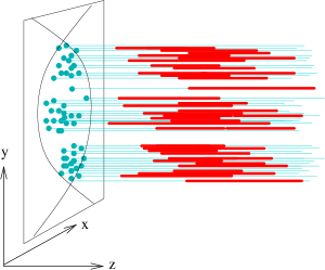
Figure 1: Macroscopic flux tubes (three in this example), made out of many individual ones, of variable length.

The longitudinal direction is along the $z$-axis, the coordinates $x$ and $y$ represent the transverse plane. A “macroscopic” flux tube is a longitudinal structure of high energy density, almost translational invariant despite an irregular form in transverse direction. Such a flux tube is made of many individual elementary flux-tubes or strings, each on having a small diameter (of 0.2 to 0.3 fm). The elementary flux tubes are actually short, the momentum fraction of the string ends are distributed roughly as $1/x$. The macroscopic flux tubes represent nevertheless long structures, simply due to the fact that many short elementary flux tubes are located at transverse positions corresponding to the positions of nucleon-nucleon scatterings. And these simply happen to be more or less frequent in certain transverse areas, as indicated in the figure by the three clusters of interaction positions (dots in the $x-y$ plane).

This flux tube approach is just a continuation of 30 years of very successful applications of the string approach to particle production in collisions of high energy particles and83 ; wer93 ; cap94 , in particular in connection with the parton model. Here, the relativistic string is a phenomenological tool to deal with the longitudinal character of the final state partonic system. An important issue at high energies is the appearance of so-called non-linear effects, which means that the simple linear parton evolution is no longer valid, gluon ladders may fuse or split. More recently, a classical treatment has been proposed, called Color Glass Condensate (CGC), having the advantage that the framework can be derived from first principles cgc1 ; cgc2 ; cgc3 ; cgc4 ; cgc5 ; cgc6 . Comparing a conventional string model like EPOS and the CGC picture: they describe the same physics, although the technical implementation is of course different. All realistic string model implementations have nowadays to deal with screening and saturation, and EPOS is not an exception. Without screening, proton-proton cross sections and multiplicities will explode at high energies. We will discuss later in more detail about the question of CGC initial conditions for hydrodynamical evolutions compared to conventional ones. To give a short answer: this question is irrelevant when it comes to event by event treatment.

Starting from the flux-tube initial condition, the system expands very rapidly, thanks to the realistic cross-over equation-of-state, flow (also elliptical one) develops earlier compared to the case a strong first order equation-of-state as in hydro2b ; hydro2c , temperatures corresponding to the cross-over (around 170 MeV) are reached in less than 10 fm/c.

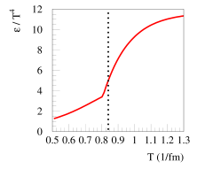
Figure 2: The energy density over $T^{4}$ as a function of the temperature $T$. The dotted line indicates the “hadronization temperature”, i.e. end of the thermal phase, when “matter” is transformed into hadrons.

The system hadronizes in the cross-over region, where here “hadronization” is meant to be the end of the completely thermal phase: matter is transformed into hadrons. We stop the hydrodynamical evolution at this point, but particles are not yet free. Our favorite hadronization temperature is 166 MeV, shown as the dotted line in fig. 2, which is indeed right in the transition region, where the energy density varies strongly with temperature. At this point we employ statistical hadronization, which should be understood as hadronization of the quark-gluon plasma state into a hadronic system, at an early stage, not the decay of a resonance gas in equilibrium.

After this hadronization –although no longer thermal– the system still interacts via hadronic scatterings, still building up (elliptical) flow, but much less compared to an idealized thermal resonance gas evolution, which does not exist in reality.

Despite the non-equilibrium behavior in the finale stage of the collision, our sophisticated procedure gives particle yields close to what has been predicted in statistical models, see fig. 3.

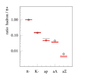
Figure 3: Particle ratios (hadron yields to $\pi^{+}$ yields) from our model calculations (thick horizontal line) as compared to the statistical model gas1 (thin horizontal line), and to data brahmsN1 ; brahmsN2 ; starNpt (points).

This is because the final hadronic cascade does not change particle yields too much (with some exceptions to be discussed later), but it affects slopes and –as mentioned– azimuthal asymmetry observables.

In the following, we will present the details of our realistic approach to the hydrodynamic evolution in heavy ion collisions, with a subsequent attempt to understand and interpret all soft heavy ion data from Au-Au at 200 GeV. The predictive power of the presented approach is enormous. The basic EPOS approach, which fixes the flux tube initial conditions, has quite a number of parameters determining soft Pomeron properties, the perturbative QCD treatment (cutoffs), the string dynamics, screening and saturation effects, the projectile and target remnant properties. All these unknowns are fixed by investigating electron-positron, proton-proton, and proton-nucleus scattering from SPS via RHIC to Tevatron energies, for all observables where data are available. This huge amount of elementary data lets very little freedom concerning heavy ion collisions.

II Elementary flux tubes and non-linear evolution

Nucleus-nucleus scattering - even proton-proton - amounts to many elementary collisions happening in parallel. Such an elementary scattering is the so-called “parton ladder” , see fig. 4, also referred to as cut Pomeron, see appendix A and kw-split .

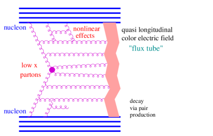
Figure 4: Elementary interaction in the EPOS model.

A parton ladder represents parton evolutions from the projectile and the target side towards the center (small $x$). The evolution is governed by an evolution equation, in the simplest case according to DGLAP. In the following we will refer to these partons as “ladder partons”, to be distinguished from “spectator partons” to be discussed later. It has been realized a long time ago that such a parton ladder may be considered as a quasi-longitudinal color field, a so-called “flux tube”, conveniently treated as a relativistic string. The intermediate gluons are treated as kink singularities in the language of relativistic strings, providing a transversely moving portion of the object. This flux tube decays via the production of quark-antiquark pairs, creating in this way fragments – which are identified with hadrons. Such a picture is also in qualitative agreement with recent developments concerning the Color Glass Condensate, as discussed earlier.

A consistent quantum mechanical treatment of the multiple scattering is quite involved, in particular when the energy sharing between the parallel scatterings is taken into account. For a detailed discussion we refer to nexus . Based on cutting rule techniques, one obtains partial cross sections for exclusive event classes, which are then simulated with the help of Markov chain techniques.

Important in particular at moderate energies (RHIC): our “parton ladder” is meant to contain two parts nexus : the hard one, as discussed above (following an evolution equation), and a soft one, which is a purely phenomenological object, parametrized in Regge pole fashion, see appendix. The soft part essentially compensates for the infrared cutoffs, which have to be employed in the perturbative calculations.

At high energies, one needs to worry about non-linear effects, because the gluon densities get so high that gluon fusion becomes important. Nonlinear effects could be taken into account in the framework of the CGC cgc1 ; cgc2 ; cgc3 ; cgc4 ; cgc5 ; cgc6 . Here , we adopt a phenomenological approach, which grasps the main features of these non-linear phenomena and still remains technically doable (we should nor forget that we finally have to deal with complications due to multiple scatterings, as discussed earlier).

Our phenomenological treatment is based on the fact that there are two types of nonlinear effects kw-split : a simple elastic rescattering of a ladder parton on a projectile or target nucleon (elastic ladder splitting), or an inelastic rescattering (inelastic ladder splitting), see figs. 5, 6. The elastic process provides screening, therefore a reduction of total and inelastic cross sections. The importance of this effect should first increase with mass number (in case of nuclei being involved), but finally saturate. The inelastic process will affect particle production, in particular transverse momentum spectra, strange over non-strange particle ratios, etc. Both, elastic and inelastic rescattering must be taken into account in order to obtain a realistic picture.

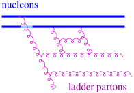
Figure 5: Elastic “rescattering” of a ladder parton.

 

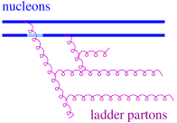
Figure 6: Inelastic “rescattering” of a ladder parton.

To include the effects of elastic rescattering, we first parametrize a parton ladder (to be more precise: the imaginary part of the corresponding amplitude in impact parameter space) computed on the basis of DGLAP. We obtain an excellent fit of the form

$$\alpha(x^{+}x^{-})^{\beta},$$ (1)

where $x^{+}$ and $x^{-}$ are the momentum fractions of the “first” ladder partons on respectively projectile and target side (which initiate the parton evolutions). The parameters $\alpha$ and $\beta$ depend on the cms energy $\sqrt{s}$ of the hadron-hadron collision. To mimic the reduction of the increase of the expressions $\alpha(x^{+}x^{-})^{\beta}$ with energy, we simply replace them by

$$\alpha(x^{+})^{\beta+\varepsilon_{P}}(x^{-})^{\beta+\varepsilon_{T}},$$ (2)

where the values of the positive numbers $\varepsilon_{P/T}$ will increase with the nuclear mass number and $\log s$. This additional exponent has very important consequences: it will reduce substantially the increase of both cross sections and multiplicity with the energy, having thus a similar effect as introducing a saturation scale.

The inelastic rescatterings (ladder splittings, looking from insider to outside) amount to providing several ladders close to the projectile (or target) side, which are close to each other in space. They cannot be considered as independent color fields (strings), we should rather think of a common color field built from several partons ladders. We treat this object via an enhancement of remnant excitations, the latter ones to be discussed in the following.

So far we just considered two interacting partons, one from the projectile and one from the target. These partons leave behind a projectile and target remnant, colored, so it is more complicated than simply projectile/target deceleration. One may simply consider the remnants to be diquarks, providing a string end, but this simple picture seems to be excluded from strange antibaryon results at the SPS sbaryons . We therefore adopt the following picture: not only a quark, but a two-fold object takes directly part in the interaction, namely a quark-antiquark or a quark-diquark pair, leaving behind a colorless remnant, which is, however, in general excited (off-shell). If the first ladder parton is a gluon or a seaquark, we assume that there is an intermediate object between this gluon and the projectile (target), referred to as soft Pomeron. And the “initiator” of the latter one is again the above-mentioned two-fold object.

So we have finally three “objects”, all of them being white: the two off-shell remnants, and the parton ladder in between. Whereas the remnants contribute mainly to particle production in the fragmentation regions, the ladders contribute preferentially at central rapidities.

We showed in ref. nex-bar that this “three object picture” can solve the “multi-strange baryon problem” of ref. sbaryons . In addition, we assembled all available data on particle production in pp and pA collisions between 100 GeV (lab) up to Tevatron, in order to test our approach. Large rapidity (fragmentation region) data are mainly accessible at lower energies, but we believe that the remnant properties do not change much with energy, apart of the fact that projectile and target fragmentation regions are more or less separated in rapidity. But even at RHIC, there are remnant contribution at rapidity zero, for example the baryon/antibaryon ratios are significantly different from unity, in agreement with our remnant implementation. So even central rapidity RHIC data allow to confirm our remnant picture.

III Flux tubes, jets, and core-corona separation

We will identify parton ladders with elementary flux tubes, the latter ones treated as classical strings. The relativistic classical string picture is very attractive, because its dynamics (Lagrangian) is essentially derived from general principles as covariance and gauge invariance (the dynamics should not depend on a particular string surface parametrization). We use the simplest possible string: a two-dimensional surfaces $X(\alpha,\beta)$ in 3+1 dimensional space-time, with piecewise constant initial conditions,

$$V(\alpha)\equiv\frac{\partial X}{\partial\beta}(\alpha,\beta=0)=V_{k},\;\mathrm{in}\>[\alpha_{k},\alpha_{k+1}],$$ (3)

referred to as kinky strings. The dynamics is governed by the Nambu-Goto string action string1 ; string2 ; string3 (see also wer93 ). Our string is characterized by a sequence of intervals $[\alpha_{k},\alpha_{k+1}]$, and the corresponding velocities $V_{k}$. Such an interval with its constant value of $V$ is referred to as “kink”. Now we are in a position to map partons onto strings: we identify the ladder partons with the kinks of a kinky string, such that the length of the $\alpha$-interval is given by the parton energies $E_{k}$, and the kink velocities are just the parton velocities, $p_{k}^{\mu}/E_{k}$. The string evolution is then completely given by these initial conditions, expressed in terms of parton momenta. The string surface is given as

$$X(\alpha,\beta)=X_{0}+\frac{1}{2}\left[\int_{\alpha-\beta}^{\alpha+\beta}V\left(\xi\right)d\xi\right].$$ (4)

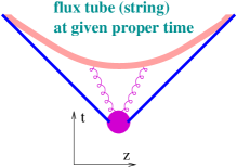
Figure 7: Flux tube (string) at given proper time. The picture is schematic in the sense that the string extends well into the transverse dimension, correctly taken into account in the calculations. The quantity $X$ is a four-vector!

Let us considers a string at a given proper time $\tau_{0}$. In fig. 7, the thick line of the form of a hyperbola represents schematically the intersection of the string surface $X(\alpha,\beta)$ with the hypersurface corresponding to constant proper time: $\tau=\tau_{0}$. We show only a simplified picture in $z-t$ space, whereas in reality (and in our calculations) all three space dimensions are important, due to the transverse motion of the kinks: the string at constant proper time is a one-dimensional manifold in the full 3+1 dimensional space-time. In fig. 8, we sketch the space components of this object: the string in $\mathrm{I\!R^{3}}$ space is a mainly longitudinal object (here parallel to the $z$-axis) but due to the kinks there are string pieces moving transversely (in $y$-direction in the picture). But despite these kinks, most of the string carries only little transverse momentum!

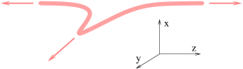
Figure 8: Flux tube with transverse kink in $\mathrm{I\!R^{3}}$ space. The kink leads to transversely moving string regions (transverse arrow).

In case of elementary reactions like electron-positron annihilation or proton proton scattering (at moderately relativistic energies), hadron production is realized via string breaking, such that string fragments are identified with hadrons. Here, we employ the so-called area law hypothesis artru ; artru2 (see also wer93 ): the string breaks via $q-\bar{q}$ or $qq-\overline{qq}$ production within an infinitesimal area $dA$ on its surface with a probability which is proportional to this area, $dP=p_{B}\,dA,$where $p_{B}$ is the fundamental parameter of the procedure. It should be noted that despite the very complicated structure of the string surface $X(\alpha,\beta)$ in 3+1 space-time, the breaking procedure following the area law can be done rigorously, using the so-called band-method nexus ; mor87 . The flavor dependence of the $q-\bar{q}$ or $qq-\overline{qq}$ string breaking is given by the probabilities $\exp(-\pi m_{q}^{2}/\kappa$), with $m{}_{q}$ being the quark masses and $\kappa$ the string tension. After breaking, the string pieces close to a kink constitute the jets of hadrons (arrows in fig. 9),

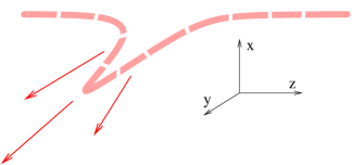
Figure 9: Broken flux tube with transverse kink in $\mathrm{I\!R^{3}}$ space. The string segments close to the kink giving rise to transversely moving hadrons, constituting a jet (arrows).

whose direction is mainly determined by the kink-gluon.

When it comes to heavy ion collisions or very high energy proton-proton scattering, the procedure has to be modified, since the density of strings will be so high that they cannot possibly decay independently kw-core . For technical reasons, we split each string into a sequence of string segments, corresponding to widths $\delta\alpha$ and $\delta\beta$ in the string parameter space (see fig. 10.

Figure 10: String segment at given proper time. The picture is schematic in the sense that the string extends well into the transverse dimension, correctly taken into account in the calculations.

One distinguishes between string segments in dense areas (more than some critical density $\rho_{0}$ of segments per unit volume), from those in low density areas. The high density areas are referred to as core, the low density areas as corona kw-core . String segments with large transverse momentum (close to a kink) are excluded from the core. At this stage, we do not consider energy loss of these kink partons, we will investigate this in a later publication. Also excluded from the core are remnant baryons. Simple implementations of the core-corona idea can be found in corecoro ; corecoro2 .

Let us consider the core part. Based on the four-momenta of infinitesimal string segments, we compute the energy momentum tensor and the flavor flow vector at some position $x$ (at $\tau=\tau_{0}$) as nex-ic

$$T^{\mu\nu}(x) = \sum_{i}\frac{\delta p_{i}^{\mu}\delta p_{i}^{\nu}}{\delta p_{i}^{0}}g(x-x_{i}),$$ (5)

$$N_{q}^{\mu}(x) = \sum_{i}\frac{\delta p_{i}^{\mu}}{\delta p_{i}^{0}}\,q_{i}\,g(x-x_{i}),$$ (6)

where $q\in{u,d,s}$ represents the net flavor content of the string segments, and

$$\delta p=\left\{\frac{\partial X(\alpha,\beta)}{\partial\beta}\delta\alpha+\frac{\partial X(\alpha,\beta)}{\partial\alpha}\delta\beta\right\}\quad$$ (7)

are the four-momenta of the segments. The function $g$ is a Gaussian smoothing kernel with a transverse width $\sigma_{\bot}$= 0.25 fm. The Lorentz transformation into the comoving frame gives

$$\Lambda^{\alpha}\,_{\mu}\Lambda^{\beta}\,_{\nu}T^{\mu\nu}=T_{\mathrm{com}}^{\mu\nu},$$ (8)

where we define the comoving frame such that the first column of $T_{\mathrm{com}}$ is of the form $(\varepsilon,0,0,0)^{T}$. This provides an equation for the energy density $\varepsilon$ in the comoving frame, and the flow velocity components $v^{i}$ :

$$\varepsilon = T^{00}-\sum_{k=1}^{3}T^{0k}v^{k}\,,$$ (9)

$$v^{i} = \frac{1}{\varepsilon}(T^{i0}-T^{ik}v^{k}),$$ (10)

which may be solved iteratively kodama ,

$$\varepsilon^{(n)} = T^{00}-\sum_{k=1}^{3}T^{0k}v^{(n-1)\,k}\,,$$ (11)

$$v^{(n)\,i} = \frac{1}{\varepsilon^{(n)}}(T^{i0}-T^{ik}v^{(n-1)\,k}).$$ (12)

The flavor density is then calculated as

$$f_{q}=N_{q}u,$$ (13)

with $u$ being the flow four-velocity.

From the above procedure, we get event-by-event fluctuations of the collective transverse velocities, but these flows are very small. However, several authors iniflo1 ; iniflo2 ; iniflo3 ; iniflo4 ; iniflo5 ; hbt-puzzle discussed recently the possibility of having already an initial collective velocity. We consider such a possibility by adding to our transverse velocities $v_{x/y}(r,\phi)$ the following terms:

$$\Delta v_{x}(r,\phi) =\min(0.4,\,v_{0}r/r_{0})\,\sqrt{1+\epsilon}\,\cos\phi,$$ (14)

$$\Delta v_{y}(r,\phi) =\min(0.4,\,v_{0}r/r_{0})\,\sqrt{1-\epsilon}\,\sin\phi,$$ (15)

with

$$r_{0}=\rho\sqrt{1-\epsilon\,\cos 2\phi},$$ (16)

and

$$\rho=4\sqrt{\left\langle x^{2}+y^{2}\right\rangle/2},\quad\epsilon=\left\langle y^{2}-x^{2}\right\rangle/\left\langle y^{2}+x^{2}\right\rangle.$$ (17)

Such an initial collective transverse flow seems to be not really essential for reproducing the data, however, a value $v_{0}=0.25$ gives a slight improvement of the transverse momentum spectra, compared to $v_{0}=0$. So we use the former value as default.

IV Hydrodynamic evolution, realistic equation-of-state

Having fixed the initial conditions, the core evolves according to the equations of ideal hydrodynamics, namely the local energy-momentum conservation

$$\partial_{\mu}T^{\mu\nu}=0,\quad\nu=0,...,3\,,$$ (18)

and the conservation of net charges,

$$\partial N_{k}^{\mu}=0,\quad k=B,S,Q\,,$$ (19)

with $B$, $S$, and $Q$ referring to respectively baryon number, strangeness, and electric charge. In this paper we treat ideal hydrodynamic, so we use the decomposition

$$T^{\mu\nu}=(\epsilon+p)\,u^{\mu}u^{\nu}-p\,g^{\mu\nu}\,,$$ (20)

$$N_{k}^{\mu}=n_{k}u^{\mu},$$ (21)

where $u$ is the four-velocity of the local rest frame. Solving the equations, as discussed in the appendix, provides the evolution of the space-time dependence of the macroscopic quantities energy density $\varepsilon(x)$, collective flow velocity $\vec{v}(x)$, and the net flavor densities $n_{k}(x)$. Here, the crucial ingredient is the equation of state, which closes the set of equations by providing the $\varepsilon$-dependence of the pressure $p$. The equation-of-state should fulfill the following requirements:

• flavor conservation, using chemical potentials $\mu_{B}$, $\mu_{S}$, $\mu_{Q}$;

• compatibility with lattice gauge results in case of $\mu_{B}=$$\mu_{S}=$$\mu_{Q}=0$.

The starting point for constructing this “realistic” equation-of-state is the pressure $p_{H}$ of a resonance gas, and the pressure $p_{Q}$ of an ideal quark gluon plasma, including bag pressure. Be $T_{c}$ the temperature where $p_{H}$ and $p_{Q}$ cross. The correct pressure is assumed to be of the form

$$p=p_{Q}+\lambda\,(p_{H}-p_{Q}),$$ (22)

where the temperature dependence of $\lambda$ is given as

$$\lambda=\exp\left(-\frac{T-T_{c}}{\delta}\right)\Theta(T-T_{c})+\Theta(T_{c}-T),$$ (23)

with

$$\delta=\delta_{0}\exp\left(-(\mu_{B}/\mu_{c})^{2}\right)\left(1+\frac{T-T_{c}}{2T_{c}}\right).$$ (24)

From the pressure one obtains the entropy density $S$ as

$$S=\frac{\partial p}{\partial T}=S_{Q}+\lambda\,(S_{H}-S_{Q})+\frac{\partial\lambda}{\partial T}\,(p_{H}-p_{Q}),$$ (25)

and the flavor densities $n^{i}$ as

$$n^{i}=\frac{\partial p}{\partial\mu^{i}}=n_{Q}^{i}+\lambda\,(n_{H}^{i}-n_{Q}^{i})+\frac{\partial\lambda}{\partial\mu^{i}}\,(p_{H}-p_{Q}).$$ (26)

The energy density is finally given as

$$\varepsilon=TS+\sum_{i}\mu^{i}n^{i}-p,$$ (27)

or

$$\varepsilon=\varepsilon_{Q}+\lambda\,(\varepsilon_{H}-\varepsilon_{Q})+\left(T\frac{\partial\lambda}{\partial T}+\mu^{i}\frac{\partial\lambda}{\partial\mu^{i}}\right)(p_{H}-p_{Q}).$$ (28)

Our favorite equation-of-state, referred to as “X3F”, is obtained for $\delta_{0}=0.15$, which reproduces lattice gauge results for $\mu_{B}=$$\mu_{S}=$$\mu_{Q}=0$, as shown in figs. 11 and 12.

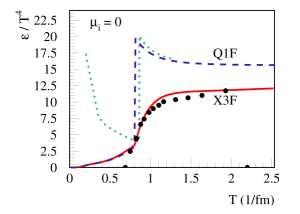
Figure 11: Energy density versus temperature, for our equation-of-state X3F (full line), compared to lattice data lattice (points), and some other EoS choices, see text.

Figure 12: Pressure versus temperature, for our equation-of-state X3F (full line), compared to lattice data lattice (points), and some other EoS choices, see text.

The symbol X3F stands for “cross-over” and “3 flavor conservation”. Also shown in the figures is the EoS Q1F, referring to a simple first order equation-of-state, with baryon number conservation, which we will use as a reference to compare with. Many current calculations are still based on this simple choice, as for example the one in hydro2b ; hydro2c , shown as dotted lines in figs. 11 and 12.

When the evolution reaches the hadronization hypersurface, defined by a given temperature $T_{\mathrm{H}}$, we switch from “matter” description to particles, using the Cooper-Frye description. Particles may still interact, as discussed below, so hadronization here means an intermediate stage, particles are not yet free streaming, but they are not thermalized any more. The hadronization procedure is described in detail in the appendix. After the “intermediate” hadronization, the particles at their hadronization positions (on the corresponding hypersurface) are fed into the hadronic cascade model UrQMD urqmd ; urqmd2 , performing hadronic interaction until the system is so dilute that no interaction occur any more. The “final” freeze out position of the particles is the last interaction point of the cascade process, or the hydro hadronization position, if no hadronic interactions occurs.

V On the importance of an event-by-event treatment

A remarkable feature of an event-by-event treatment of the hydrodynamical evolution based on random flux tube initial conditions is the appearance of a so-called ridge-structure, found in Spherio calulations based on Nexus initial conditions ridge1 ; ridge2 . We expect to observe a similar structure doing an event-by-event hydrodynamical evolution based on flux-tube initial conditions from EPOS. The result is shown in fig. 13, where we plot the dihadron

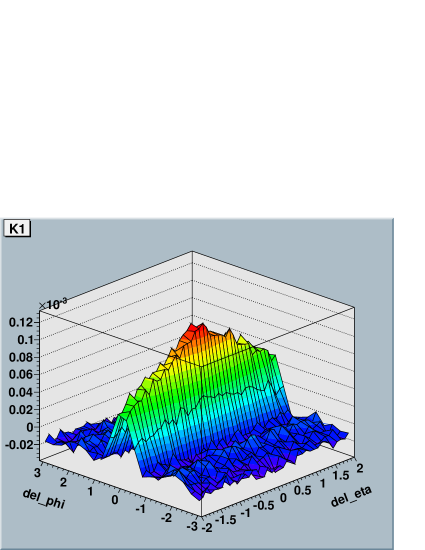
Figure 13: Dihadron $\Delta\eta\,-\,\Delta\phi$ correlation in a central Au-Au collision at 200 GeV, as obtained from an event-by-event treatment of the hydrodynamical evolution based on random flux tube initial conditions. Trigger particles have transverse momenta between 3 and 4 GeV/c, and associated particles have transverse momenta between 2 GeV/c and the $p_{t}$ of the trigger.

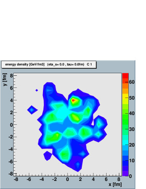
Figure 14: Initial energy density in a central Au-Au collision at 200 GeV, at a space-time rapidity $\eta_{s}=0$.

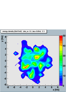
Figure 15: Initial energy density in a central Au-Au collision at 200 GeV, at a space-time rapidity $\eta_{s}=1.5$.

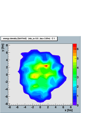
Figure 16: Energy density at a proper time $\tau=2.6\,$fm/c, at a space-time rapidity $\eta_{s}=0$.

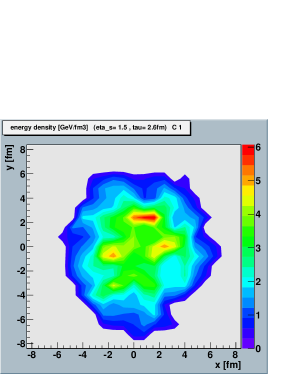
Figure 17: Energy density at a proper time $\tau=2.6\,$fm/c, at a space-time rapidity $\eta_{s}=1.5$.

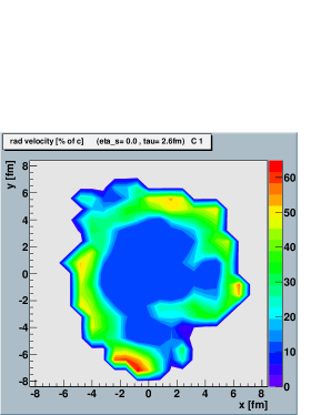
Figure 18: Radial flow velocity at a proper time $\tau=2.6\,$fm/c, at a space-time rapidity $\eta_{s}=0$.

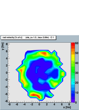
Figure 19: Radial flow velocity at a proper time $\tau=2.6\,$fm/c, at a space-time rapidity $\eta_{s}=1.5$.

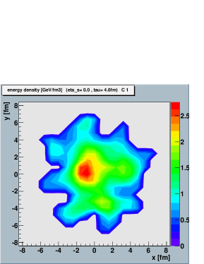
Figure 20: Energy density at a proper time $\tau=4.6\,$fm/c, at a space-time rapidity $\eta_{s}=0$.

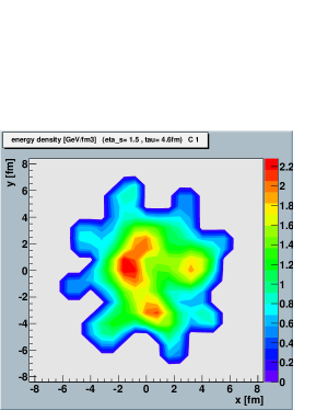
Figure 21: Energy density at a proper time $\tau=4.6\,$fm/c, at a space-time rapidity $\eta_{s}=1.5$.

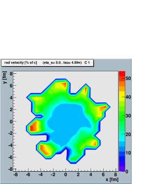
Figure 22: Radial flow velocity at a proper time $\tau=4.6\,$fm/c, at a space-time rapidity $\eta_{s}=0$.

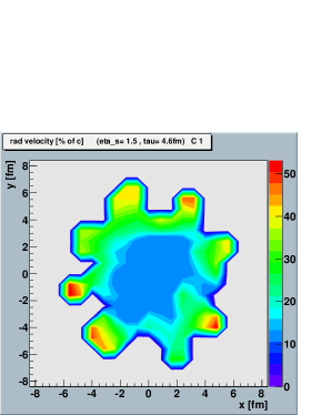
Figure 23: Radial flow velocity at a proper time $\tau=4.6\,$fm/c, at a space-time rapidity $\eta_{s}=1.5$.

correlation $dN/d\Delta\eta\,d\Delta\phi$, with $\Delta\eta$ and $\Delta\phi$ being respectively the difference in pseudorapidity and azimuthal angle of a pair of particles. Here, we consider trigger particles with transverse momenta between 3 and 4 GeV/c, and associated particles with transverse momenta between 2 GeV/c and the $p_{t}$ of the trigger, in central Au-Au collisions at 200 GeV. Our ridge is very similar to the structure observed by the STAR collaboration ridge .

In the following we will discuss a particular event, which can, however, be considered as a typical example, with similar observations being true for randomly chosen events. Important for understanding the strong $\Delta\eta$ – $\Delta\phi$ correlation is the observation, that the initial energy density has a very bumpy structure as a function of the transverse coordinates $x$ and $y$. However, this irregular structure is the same at different longitudinal positions. This can be clearly seen in figs. 14 and 15, where we show for a given event the energy density distributions in the transverse planes at different space-time rapidities, namely $\eta_{s}=0$ and $\eta_{s}=1.5$: we observe almost the same structure. For different events, the details of the bumpy structures change, but we always find an approximate “translation invariance”: the distributions of energy density in the transverse planes vary only little with the longitudinal variable $\eta_{s}$. It should be noted that the colored areas represent only the interior of the hadronization surface, the outside regions are white. Hadronization is meant to be an intermediate step, before the hadronic cascade. An approximate translational invariance is also observed when we go to larger values of $\eta_{s}$, so for example when we compare the energy density at $\eta_{s}=1.5$ with the one at $\eta_{s}=3.0$: the form of the energy distributions is similar, however, the magnitude at large $\eta_{s}$ is smaller.

Considering later times, we see in figs. 16 to 19, that the approximate translational invariance is conserved, for both energy densities and radial flow velocities. It is remarkable (and again true in general, for arbitrary events) that the energy distribution in the transverse plane is much smoother than initially, the distribution looks more homogeneous. Very important for the following discussion is the flow pattern, seen in figs. 18 and 19, for $\eta_{s}=0$ and $\eta_{s}=1.5$ : the radial flow is as expected largest in the outer regions. Closer inspection of the outside ring of large radial flows reveals an irregular atoll-like structure: there are well pronounced peaks of large flow over the background ring. At even later times, as seen in figs. 20 to 23, the outer surfaces get irregular, due to the irregular flows discussed above, again with well identified peaks of large radial flows.

The well isolated peaks of the radial flow velocities have two important properties: they sit close to the hadronization surface, and they sit at the same azimuthal angle, when comparing different longitudinal positions $\eta_{s}$. As a consequence, particles emitted from different longitudinal positions get the same transverse boost , when their emission points correspond to the azimuthal angle of a common flow peak position. And since longitudinal coordinate and (pseudo)rapidity are correlated, one obtains finally a strong $\Delta\eta$ – $\Delta\phi$ correlation.

(a)

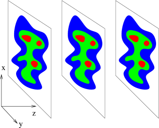
(b)

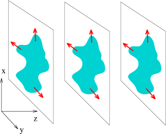
Figure 24: Schematic view of the translational invariance of the initial energy density (a), leading to a corresponding invariance of the transverse flow. We use the term “invariance” in the sense of a similarity transform: same shape, but different magnitude. The magnitude of the energy density at large $\eta_{s}$ is of course smaller than the one at $\eta_{s}=0$.

In fig. 24, we summarize the above discussion: the flux tube initial conditions provide a bumpy structure of the energy density in the transverse plane, which shows, however, an approximate translational invariance (similar behavior at different longitudinal coordinates). Solving the hydrodynamic equations preserves this invariance, leading in the further evolution to an invariance of the transverse flow velocities. These identical flow patterns at different longitudinal positions lead to the fact that particles produced at different values of $\eta_{s}$ profit from the same collective push, when they are emitted at an azimuthal angle corresponding to a flow maximum (indicated by the arrows in the figure).

Finally we have to address the question, why we have a irregular transverse structure with an approximate translational invariance. The basic structure of EPOS is such that each individual nucleon-nucleon collision results in a projectile and target remnant, and two or more elementary flux tubes (strings). The higher the energy the bigger the number of strings. Most of the energy of the reaction is carried by the remnants, the flux tubes cover only a limited range in rapidity, but their “lengths” (in rapidity) vary enormously. Nevertheless we obtain a very smooth variation of the energy density with the longitudinal coordinate $\eta_{s}$. This is due to the fact that the transverse positions of a string is given by the position of the nucleon pair, who’s interaction gave rise the the formation of the flux tube. These “pair positions” fluctuate considerably, event-by-event, and one obtains typically

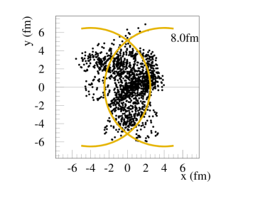
Figure 25: Projection of the positions of nucleon-nucleon scattering to the transverse ($x,y$) plane, from a simulation of a semi-peripheral ($b=8$fm/c) Au-Au event at 200 GeV.

Figure 26: Schematic view of the projection of the positions of nucleon-nucleon scattering to the transverse ($x,y$) plane, which defines “possible transverse positions” of the flux tubes, indicated by the thin lines. The actual flux tubes fluctuate concerning their longitudinal positions; a possible realization is shown by the thick lines.

a situation as shown in fig. 25, where we plot the projection to the transverse plane of the positions of the interaction nucleon-nucleon pairs. The two circles representing two hard sphere nuclei is only added to guide the eye, for the calculations we use of course a realistic nuclear density. Clearly visible in the figure is the inhomogeneous structure: there are areas with a high density of interaction points, and areas which are less populated. These transverse positions of interacting pairs define also the corresponding positions of the flux tubes associated to the pairs. In fig. 26, we present a schematic view of this situation: on the left we plot the pair positions projected to the transverse plane (dots). From each dot we draw a line parallel to the $z$–axis, representing a possible location of a flux tube. The flux tubes have variable longitudinal lengths, they do not cover the full possible length between projectile and target, but only a portion, as indicated by the thick horizontal lines in the figure. But even then, the transverse structure (minima and maxima of the energy density) is to a large extend determined by the density of nucleon-nucleon pairs.

VI Elliptical flow

Important information about the space-time evolution of the system is provided by the study of the azimuthal distribution of particle production. One usually expands

$$\frac{dn}{d\phi}\propto 1+2\,v_{2}\,\cos 2\phi+...\,,$$ (29)

where a non-zero coefficient $v_{2}$ is referred to as elliptical flow ollitrault . It is usually claimed that the elliptical flow is proportional to the initial space eccentricity

$$\epsilon=\frac{\left\langle y^{2}-x^{2}\right\rangle}{\left\langle y^{2}+x^{2}\right\rangle}.$$ (30)

We therefore plot in fig. 27

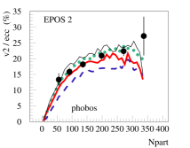
Figure 27: Centrality dependence of the ratio of $v_{2}$ over eccentricity. Points are data phobosv2ecc , the different curves refer to the full calculation – hydro & cascade (full line), only elastic hadronic scatterings (dotted), and no hadronic cascade at all (dashed). The thin solid line –above all others– refers to the hydrodynamic calculation till final freeze-out at 130 MeV.

the ratio of $v_{2}$ over eccentricity. The points are data; the full line is the full calculation: hydrodynamical evolution with subsequent hadronic cascade, from flux tube initial conditions, in event-by-event treatment. The dotted line refers to a simplified hadronic cascade, allowing only elastic scatterings, the dashed line is the calculation without hadronic cascade. In all cases, hadronization from the thermal phase occurs at $T_{\mathrm{H}}=166\,$MeV. We also show as thin solid line the hydrodynamic calculation till final freeze-out at 130 MeV. We use an energy density weighted average for the computation of the eccentricity. For both $v_{2}$ and $\epsilon$, we take into account the fact that the principle axes of the initial matter distribution are tilted with respect to the reaction plane. So we get non-zero values even for very central collisions, due to the random fluctuations.

For all theoretical curves, the ratio $v_{2}/\epsilon$ is not constant, but increases substantially from peripheral towards central collisions – in agreement with the data. In our case, this increase is a core-corona effect: for peripheral collisions (small number of participating nucleons $N_{\mathrm{part}}$), the relative importance of corona to core increases, and since the corona part does not provide any $v_{2}$, one expects roughly corecoro3

$$\frac{v_{2}}{\epsilon}=f_{\mathrm{core}}(N_{\mathrm{part}})\cdot\left.\frac{v_{2}}{\epsilon}\right|_{\mathrm{core}},$$ (31)

with a monotonically increasing relative core weight $f_{\mathrm{core}}(N_{\mathrm{part}})$, which varies between zero (very peripheral) and unity (very central). Comparing the theoretical curves in fig. 27, we see that most elliptical flow is produced early, as seen by the dashed line, representing an early freeze out – at $T_{\mathrm{FO}}=T_{\mathrm{H}}=166\,$MeV. Adding final state hadronic rescattering leads to the full curve (full cascade) or the dotted one (only elastic scattering), adding some more 20 % to $v_{2}$. The difference between the two rescattering scenarios is small, which means the effect is essentially due to elastic scatterings. Continuing the hydrodynamic expansion through the hadronic phase till freeze out at a low temperature ($130$MeV), instead of employing a hadronic cascade, we obtain a even higher elliptic flow, as shown by the thin line in fig. 27, and as discussed already inhydro2b ; hydro2c ; beijing08 .

We now discuss the effect of the equation of state (see also hydro1f ). Using a (non-realistic) first-order equations of state (curve Q1F from fig. 11), one obtains considerably less elliptical flow compared to the calculation using the the cross-over equation of state X3F, as seen in fig. 28.

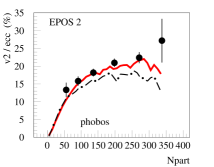
Figure 28: Centrality dependence of the ratio of $v_{2}$ over eccentricity, for a full calculation, hydro & hadronic cascae, for a (non-realistic) first-order transition equations of state (dashed-dotted line) compared to the cross-over equations of state, the default case (full line, same as the one in fig. 27). Points are data phobosv2ecc .

Taking a wrong equation-of-state and a wrong treatment of the hadronic phase (thermally equilibrated rather than hadronic cascade) compensate each other, concerning the elliptical flow results.

In our realistic (ideal) hydrodynamical treatment we get always an increase of the ratio of $v_{2}$ over eccentricity, whereas it is also claimed that this variation is due to incomplete thermalization ollitrault2 .

More detailed information is obtained by investigating the (pseudo)rapidity dependence of the elliptical flow, for different centralities, as shown in fig. 29 for Au-Au scattering at 200 GeV.

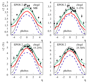
Figure 29: Pseudorapidity distributions of the elliptical flow $v_{2}$ for minimum bias events (upper left) and different centrality classes, in Au-Au collisions at 200 GeV. Points are data phobosv2 , the different curves refer to the full calculation – hydro & cascade (full thick line), only elastic hadronic scatterings (dotted), no hadronic cascade at all (dashed), and hydrodynamic calculation till final freeze-out at 130 MeV (thin line).

Again we compare several scenarios: the full treatment, namely hydrodynamic evolution from flux tube initial conditions with early hadronization (at 166 MeV) and subsequent hadronic cascade, and the calculations with only elastic rescattering, or no hadron scattering at all. Also shown as thin line is the case where the hydrodynamic expansion is continued through the hadronic phase till freeze out at a low temperature ($130$MeV), instead of employing a hadronic cascade. The previously found observations are confirmed: at central rapidity, most flow develops early, the non-equilibrium hadronic phase gives only a moderate contribution. At large rapidities, however, the hadronic rescattering has a big relative effect on $v_{2}$. Remarkable is the almost triangular shape of our $v_{2}$ rapidity dependencies. This is partly due to the fact that the initial energy density is provided by flux tubes, each one covering a certain width in (space-time) rapidity, as indicated in fig. 26. A single elementary flux tube contributes a constant energy density in a given interval,where the interval always contains rapidity zero. If (for a simple argument) the positive string endpoints were distributed uniformly in rapidity between zero and $\eta_{s}^{\mathrm{max}}$, the energy density would be of the triangular form

$$d\epsilon/d\eta_{s}\propto\eta_{s}^{\mathrm{max}}-\eta_{s},$$ (32)

what we observe approximately. This initial shape in space-time rapidity $\eta_{s}$ seems to be mapped to the pseudo-rapidity dependence of $v_{2}$.

Also important for this discussion is the fact that the relative corona contribution is larger at large rapidities compared to small ones. The corona contributes to particle production (visible in rapidity spectra), but not to the elliptical flow.

The above $v_{2}$ results we obtained by averaging over transverse momenta $p_{t}$, with the dominant contribution coming from small transverse momenta. The $p_{t}$ dependencies of $v_{2}$ for different particle species is shown in fig. 30 (for minimum bias Au-Au collisions) and 31 (for the 20-60% most central Au-Au collisions), where we compare our simulations for pions, kaon, and protons with experimental data.

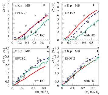
Figure 30: The transverse momentum dependence of $v_{2}$ for pions (circles, full lines), kaons (squares, dashed lines), and protons (triangles, dotted lines) for minimum bias events in minimum bias Au-Au collisions at 200 GeV. The symbols refer to datastarv2 ; phenixv2 , the lines to our full calculations.

Figure 31: The transverse momentum dependence of $v_{2}$ for pions (circles, full lines), kaons (squares, dashed lines), and protons (triangles, dotted lines) for the 20-60% most central events in Au-Au collisions at 200 GeV. The symbols refer to dataphenixv2b , the lines to our full calculations.

We first look at the results for the transverse momentum dependence of $v_{2}$ for the calculations without hadronic cascade (w/o HC), i.e. the upper left plots in figs. 30 and 31. The pion and kaon curves are almost identical, the protons are shifted, due to an important corona contribution (considering only core, all three curves are on top of each other). Turning on the final state hadronic cascade (upper right plots) will provide the mass splitting as observed in the data. Although this mass splitting was considered a great success of the hydro approach, it is in reality provided by the (non-thermal) hadronic rescattering procedure. It is this final state hadronic rescattering which is responsible for the fine structure of the $p_{t}$ dependence, although the magnitude of the integrated $v_{2}$ is produced in the early phase. The lower panel of the figs. 30 and 31 shows a somewhat different presentation of the same results: here we plot the scaled quantity $v_{2}/n_{q}$ versus the scaled kinetic energy $(m_{t}-m)/n_{q}$, where $n_{q}$ is the number of quarks of the corresponding hadron (2 for mesons, 3 for baryons). We show again the calculation without (left) and with (right) hadronic cascade. And surprisingly it is this final state hadronic rescattering which makes the three curves for pions, kaons, and protons coincide. At least in the small $p_{t}$ region considered here, the key for understanding “$v_{2}$scaling” is the hadronic cascade, not the partonic phase.

VII Glauber or Color Glass initial conditions

There has been quite some discussion in the literature concerning the possibility of increasing the elliptical flow when using Color Glass Condensate initial conditions rather then Glauber ones cgcini1 ; cgcini2 . The latter ones are usually based on a simple Ansatz, assuming that the energy density is partly proportional to the participants and partly to the binary scatterings.

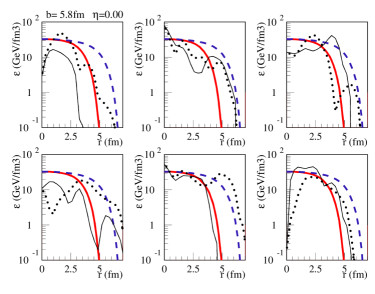
Figure 32: Initial energy density as a function of the radius $r$ for azimuthal angles $\phi=0$ and $\phi=\pi/2$, from six randomly chosen flux tube initial conditions (full thin line: $\phi=0$, dotted thin line: $\phi=\pi/2$) and from Color Glass Condensate initial conditions (full line: $\phi=0$, dashed line: $\phi=\pi/2$), for a semi-peripheral Au-Au collision.

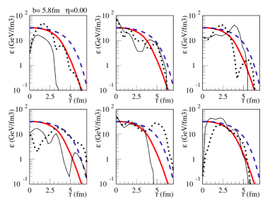
Figure 33: Initial energy density as a function of the radius $r$ for azimuthal angles $\phi=0$ and $\phi=\pi/2$, from six randomly chosen flux tube initial conditions (full thin line: $\phi=0$, dotted thin line: $\phi=\pi/2$) and from Color Glass Condensate initial conditions (full line: $\phi=0$, dashed line: $\phi=\pi/2$), for a semi-peripheral Au-Au collision.

In our case, we compute partial cross sections, which gives us the number of strings (elementary flux tubes) per nucleon-nucleon collision. So we have as well contributions proportional to the binary scatterings (the string contributions), in addition to the remnant excitations, being proportional to the participants. On the other hand, we do consider high parton density effects, introducing screening. In addition, the hydrodynamic expansion only concerns the core, and cutting off the corona pieces will produce sharper edges of the radial energy density distribution. In fig. 32, we compare the energy density distributions as obtained from a CGC calculation hydro2b ; cgcini3 , with six randomly chosen different events from our flux tube initial condition, after removing the corona. In fig. 33, we compare the same distributions from the same same six individual events to calculations from Glauber initial conditions hydro2b ; cgcini3 . Seeing these large event-by-event fluctuations, it is difficult to imagine that the differences between CGC results and Glauber are an issue when doing event-by-event treatment..

VIII Transverse momentum spectra and yields

We have discussed so-far very interesting observables like two-particle correlations and elliptical flow. However, we can only make reliable conclusions when we also reproduce elementary observables like simple transverse momentum ($p_{t}$) spectra and the integrated particle yields, for identified hadrons. We will restrict the following $p_{t}$ spectra to values less than 1.5 GeV (2 GeV in some cases), mainly in order to limit the ordinate to three or at most four orders of magnitude, which allows still to see 10% differences between calculations and data.

In the upper panel of fig. 34, we show the $p_{t}$ spectra of $\pi^{+}$(left) and $\pi^{-}$ (right) in central Au-Au collisions, for rapidities (from top to bottom) of 0, 2, and 3. The middle panels show the transverse momentum / transverse mass spectra of $\pi^{+}$ and $\pi^{-}$, for different

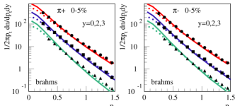
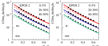
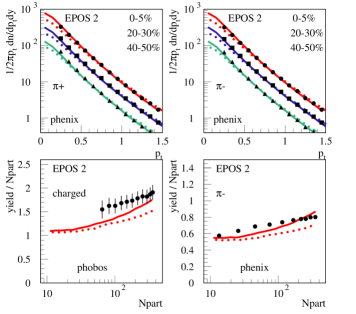
Figure 34: Production of pions in Au-Au collisions at 200 GeV. Upper panel: transverse momentum spectra for central collisions at different rapidities (from top to bottom: 0, $2$, $3$). The lower curves are scaled by factors of 1/2 and 1/4, for better visibility. Middle panels: transverse momentum (mass) distributions at rapidity zero for different centrality classes: from top to bottom: the 0-5%, the 20-30%, and the 40-50% most central collisions. Lower panel: the centrality dependence of the integrated yields for charged particles and pions. The symbols refer to data brahmspt ; starmt ; phenixptN ; phobosN , the full lines to our full calculations, the dotted lines to the calculations without hadronic cascade.

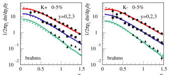
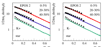
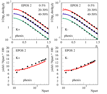
Figure 35: Same as fig. 35, but for kaons.

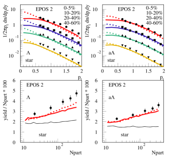
Figure 36: Production of lambdas (left) and antilambdas (right) in Au-Au collisions at 200 GeV. Upper panel: transverse momentum distributions at rapidity zero for different centrality classes: from top to bottom: the 0-5%, the 20-30%, and the 40-50% most central collisions. The lower curves are scaled by factors of 1/2, 1/4, and 1/8, for better visibility. Lower panel: the centrality dependence of the integrated yields. The symbols refer to data starNpt , the full lines to our full calculations, the dotted lines to the calculations without hadronic cascade. The thin line refers to a hydrodynamic calculation till final freeze-out at 130 MeV.

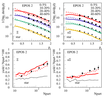
Figure 37: Same as fig. 36, but for $\Xi$ and $\bar{\Xi}$.

centralities, and the lower panel the centrality dependence of the integrated particle yields per participant for charged particles and $\pi^{-}$ mesons. In fig. 35, we show the corresponding results for kaons. In the upper panels, for the $y=2$ and $y=3$ curves, we apply scaling factors of 1/2 and 1/4, for better visibility, all other curves are unscaled. We present always two calculations: the full one (full lines), namely hydrodynamic evolution plus final state hadronic cascade, and the calculation without cascade (dotted lines). There is a slight increase of pion production in particular at low $p_{t}$ during the hadronic rescattering phase, but the difference between the two scenarios is not very big. We see almost no difference between between the calculation with and without hadronic rescattering in case of kaons. For both, pions and kaons, we observe a change of slope of the $p_{t}$ distributions with rapidity. Concerning the centrality dependence, we observe an increase of the yields per participant.

In fig. 36 and 37, we show $p_{t}$ spectra and centrality dependence of particle yields per participant, for the (multi)strange baryons $\Lambda$, $\bar{\Lambda}$, $\Xi$, and $\bar{\Xi}$. Same conventions as for the previous plots. Here we see a big effect due to rescattering: for the lambdas, the yields are not affected too much, but the $p_{t}$ spectra get much softer, when comparing the full calculation with the one without rescattering. Similarly the slopes for the $\Xi$, and $\bar{\Xi}$ get softer due to rescattering.

We also show in the lower panels of figs. 36 and 37 the yields per participant in case of a hydrodynamic calculation till final freeze-out at 130 MeV (thin lines). We have almost no centrality dependence, in contrast to the significant increase seen in the data, for both, lambdas and xis. Such a full thermal scenario with late freeze-out is therefore incompatible with strange baryon data.

For xis, the softening of $p_{t}$ spectra due to hadronic rescattering is more pronounced for the antiparticles – an absorption effect. Even the total integrated yields are affected: rescattering will reduce the $\Xi$ yields and increase the $\bar{\Xi}$ yields with centrality.

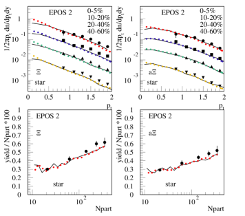
Figure 38: Same as fig. 37, but comparing the calculation without hadronic cascade (dotted) with the one with only elastic hadronic rescattering (full thin line).

Maybe too much absorption? In fig. 38, we replace the full hadronic cascade by an option where only elastic rescattering is allowed (full lines). The dotted line refers to the calculation without rescattering, as in the previous plots. Here – by definition – the yields are unchanged, only the slopes are affected. It seems that this option reproduces the data better than the full cascade.

In any case, the effect of rescattering decreases with decreasing centrality: the interaction volume simply gets smaller and smaller, reducing the possibility of rescattering.

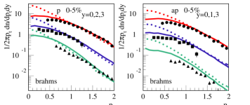
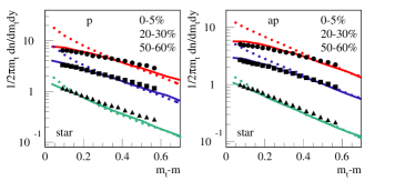
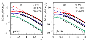
Figure 39: Transverse momentum spectra of protons (left) and antiprotons (right) in Au-Au collisions at 200 GeV. Upper panel: spectra for central collisions at different rapidities (from top to bottom: 0, $2$, $3$). The lower curves are scaled by factors of 1/2 and 1/4, for better visibility. Middle and lower panels: transverse momentum (mass) distributions at rapidity zero for different centrality classes: from top to bottom: the 0-5%, the 20-30%, and the 40-50% most central collisions. The symbols refer to databrahmspt ; phenixptN ; starNpt , the full lines to our full calculations, the dotted lines to the calculations without hadronic cascade.

We finally discuss proton and antiproton production. When talking about spectra of identified hadrons, it is implicitly assumed that these spectra do not contain contamination from weak decays, so the experimental spectra should be feed-down corrected – which is not always the case. This is in particular important for protons, strongly affected by feed-down from lambda decays. So whenever we compare to data, we adopt the same definitions: in case of feed-down correction of the data, we suppress weak resonance decays, and in case of no feed-down correction, we do let them decay. So for the following discussion, in case of the STAR data we compare to, protons are contrary to the pions not corrected, we include weak decay products. When comparing to PHENIX and BRAHMS data, we suppress weak decays. In fig. 39, we show the the proton and antiproton transverse momentum spectra at different rapidities and different centralities, for Au-Au collisions at 200 GeV. Again we show the full calculation (full lines) and the one without hadronic cascade (dotted lines). There is a huge difference between the two calculations, so proton production is very strongly affected by the hadronic cascade. Not only the slopes change, also the total yields are affected.

To summarize the above discussion on yields and $p_{t}$ spectra: an early hadronization at 166 MeV gives a reasonable description of the particle yields, which are not much affected by the hadronic final state rescattering, except for the protons. The main effect of the hadronic cascade is a softening of the $p_{t}$ spectra of the baryons.

IX Femtoscopy

All the observables discussed so-far are strongly affected by the space-time evolution of the system, nevertheless we investigate the momentum space, and conclusions about space-time are indirect, as for example our conclusions about early hadronization based on particle yields and elliptical flow results. A direct insight into the space-time structure at hadronization is obtained from using femtoscopical methods hbt3 ; hbt4 ; hbt5 ; hbt6 ; hbt7 , where the study of two-particle correlations provides information about the source function $S(\mathbf{P},\mathrm{\mathbf{r}^{\prime}})$, being the probability of emitting a pair with total momentum $\mathbf{P}$ and relative distance $\mathrm{\mathbf{r}^{\prime}}$. Under certain assumptions, the source function is related to the measurable two-particle correlation function $C(\mathbf{P},\mathbf{q})$ as

$$C(\mathbf{P},\mathbf{q})=\int d^{3}r^{\prime}\,S(\mathbf{P},\mathbf{r}^{\prime})\left|\Psi(\mathbf{q}^{\prime},\mathbf{r}^{\prime})\right|^{2},$$ (33)

with $\mathbf{q}$ being the relative momentum, and where $\Psi$ is the outgoing two-particle wave function, with $\mathbf{q}^{\prime}$ and $\mathbf{r}^{\prime}$ being relative momentum and distance in the pair center-of-mass system. The source function $S$ can be obtained from our simulations, concerning the pair wave function, we follow hbt-lednicki , some details are given in appendix F.

As an application, we investigate $\pi^{+}$– $\pi^{+}$ correlations. Here, we only consider quantum statistics for $\Psi$, no final state interactions, to compare with Coulomb corrected data. To compute the discretized correlation function $C_{ij}=C(\mathbf{P}_{i},\mathbf{q}_{j})$, we do our event-by-event simulations, and compute for each event $C^{\prime}_{ij}=\sum_{pairs}\left|\Psi(\mathbf{q}^{\prime},\mathbf{r}^{\prime})\right|^{2}$, where the sum extends over all $\pi^{+}$ pairs with $\mathbf{P}$ and $\mathbf{q}$ within elementary momentum-space-volumes at respectively $\mathbf{P}_{i}$ and $\mathbf{q}_{j}$. Then we compute the number of pairs $N_{ij}$ for the corresponding pairs from mixed events, being used to obtain the properly normalized correlation function $C_{ij}=C^{\prime}_{ij}/N_{ij}$. The correlation function will be parametrized as

$$C(\mathbf{P},\mathbf{q})=$$ (34)

$$\quad 1+\lambda\,\exp\left(-R_{\mathrm{out}}^{2}\,q_{\mathrm{out}}^{2}-R_{\mathrm{side}}^{2}\,q_{\mathrm{side}}^{2}-R_{\mathrm{long}}^{2}\,q_{\mathrm{long}}^{2}\right),$$

where "long" refers to the beam direction, "out" is parallel to projection of $\mathrm{\mathbf{P}}$ perpendicular to the beam, and "side" is the direction orthogonal to "long" and "out" fto-coord1 ; fto-coord2 ; fto-coord3 . In fig. 40, we show the results for the fit parameters $\lambda$, $R_{\mathrm{out}}$, $R_{\mathrm{side}}$, and $R_{\mathrm{long}}$, for five different centrality classes and for four $k_{T}$ intervals defined as (in MeV): KT1$=[150,250]$, KT2$=[250,350]$, KT3$=[350,450]$, KT4$=[450,600]$, where $k_{T}$ of the pair is defined as

$$k_{T}=\frac{1}{2}\left(|\vec{p}_{T}(\mathrm{pion}\,1)+\vec{p}{}_{T}(\mathrm{pion}\,2)|\right).$$ (35)

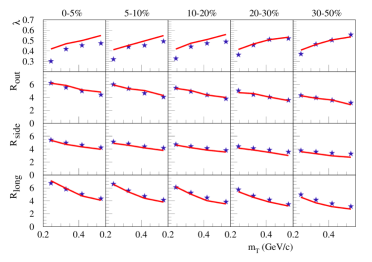
Figure 40: Femtoscopic radii $R_{\mathrm{out}}$, $R_{\mathrm{side}}$, and $R_{\mathrm{long}}$, as well as $\lambda$ as a function of $m_{T}$ for different centralities (0-5% most central, 5-10% most central, and so on). The full lines are the full calculations (including hadronic cascade), the stars data starhbt

Despite what appears in starhbt , this is the correct definition of $k_{T}$ used by STAR in their analysis lisa . The results are plotted as a function of $m_{T}=\sqrt{k_{T}^{2}+m_{\pi}^{2}}$. The model describes well the radii, the experimental lambda values are sightly below the calculations, maybe due to particle misidentification. Both data and theory provide lambda values well below unity, maybe due to pions from long-lived resonances. Concerning the $m_{T}$ dependence of the radii, we observe the same trend as seen in the data starhbt : all radii decrease with increasing $m_{T}$, and the radii decrease as well with decreasing centrality. This can be traced back to the source functions, shown in fig 41.

Figure 41: The source functions as obtained from our simulations, for three different centralities (0-5% most central, 10-20% most central, and 30-50% most central), representing the distribution of the space separation of the emission points of the pairs, in the "out" – "side" – "long" coordinate system, in the longitudinal comoving frame. The different curves per plot correspond to the different $k_{T}$ bins, see text.

These source functions are by definition the distributions of the distances $x_{i}(\mathrm{pion}\,1)-x_{i}(\mathrm{pion}\,2)$ of the pairs, where $x_{i}$ are coordinates of the emission points. We use the "out" – "side" – "long" coordinate system, and the longitudinal comoving reference frame. To account for the fact that only small values of the magnitude of the relative momentum $|\mathrm{\mathbf{q}}|$ provide a non-trivial correlation, we only count pairs with $|\mathrm{\mathbf{q}}|<75\,$MeV. The different curves per plot correspond to the different values of $k_{T}$ bins: the upper curve (full red) correspond to KT1, the second curve from the top (dashed blue) correspond to KT2, and so on. In other words, the curves get narrower with increasing $k_{T}$, which is perfectly consistent with the decreasing radii in fig. 40. Concerning the centrality dependence, the curves get narrower with decreasing centrality, in agreement with decrease of radii with decreasing centrality seen in fig. 40.

The reason for the decrease of radii with $m_{T}$ is the strong space–momentum correlation. In fig. 42,

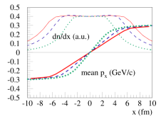
Figure 42: The mean transverse momentum component $p_{x}$ of $\pi^{+}$ as a function of the $x$ coordinate of the emission point. Also shown is the number of produced $\pi^{+}$ as a function of $x$. The different curves refer to different centralities: 0-5% = full line, 10-20% = dashed, 30-50% = dotted.

we show the average $p_{x}$ of produced $\pi^{+}$ mesons as a function of the $x$ coordinate of their formation positions, for different centralities. Clearly visible is the strong $x-p_{x}$ correlation, being typical for radial flow. Also visible in the figure is the smaller spatial extension for peripheral compared to central collisions. To illustrate this phenomenon, we show in fig. 43 a situation of completely radial transverse momentum vectors, who’s magnitudes increase with increasing distance from the center.

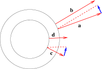
Figure 43: Radial flow effect on $m_{t}$ dependence of femtoscopic radii.

We consider two pairs of momentum vectors, $\mathbf{a}$ and $\mathbf{b}$ at some distance $r_{1}$ as well as $\mathbf{c}$ and $\mathbf{d}$ at some distance $r_{2}<r_{1}$. We have chosen the pairs such that the magnitude of their differences is the same (and “small”), to mimic the fact that only pairs with small relative momentum are relevant for the HBT analysis. The spatial distance between the two momentum vectors $\mathbf{c}$ and $\mathbf{d}$ is bigger than the one for the pair $\mathbf{a}$ and $\mathbf{b}$, due to the fact that the latter vectors are longer than the former ones ($|a|\approx|b|>|c|\approx|d|$). In this way we understand the connection between increasing $m_{t}$ and decreasing space separation.

We now consider two other scenarios: the calculation without hadronic cascade (final freeze out at 166 MeV), and the fully thermal scenario, where we continue the hydrodynamical evolution till a late freeze-out at 130 MeV (and no cascade afterwards either). In figs. 44 and 45, we see a similar space–momentum correlation as for the complete calculation in fig. 42:

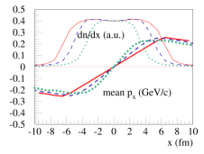
Figure 44: Same as fig. 42, but for the calculation without hadronic cascade.

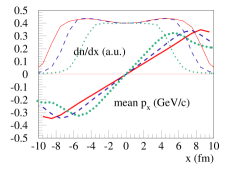
Figure 45: Same as fig. 42, but for the full thermal scenario (freeze-out at 130 MeV.

the mean transverse momentum components $p_{x}$ is roughly a linear function of the transverse coordinate $x$, in the region where the particle density is non-zero. The maximum mean $p_{x}$ is smaller in the no-cascade case, and bigger in the fully thermal case, as compared to the complete calculation. Interesting are the $dn/dx$ distributions: the no-cascade results (with early hadronization) are much narrower than the full thermal ones. The complete calculation of fig. 42 is in-between, in the sense that the plateau of the $dn/dx$ distribution is similar to the no-cascade case, but the tails are much wider.

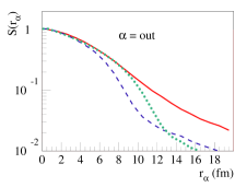
Figure 46: The source function for the "out" coordinate for the three scenarios: complete calculation, with hadronic cascade (full line), calculation without hadronic cascade and therefore final hadronization at 166 MeV (dashed), and full thermal scenario with hydrodynamic evolution till the final freeze-out at 130 MeV (dotted).

In fig. 46, we compare the source functions for the three scenarios, namely the complete calculation, the calculation without hadronic cascade, and the full thermal scenario with hydrodynamic evolution till the final freeze-out. For small values of $r_{\mathrm{out}}$, the "complete calculation" and the "full thermal" one coincide – as do the total widths of the single particle source functions $dn/dx$. For large values of $r_{\mathrm{out}}$, the "full thermal" scenario and the one "without cascade" coincide – as do the shapes of the tails of the single particle source functions. A similar behavior is found for all the source functions, as shown in figs. 47 and 48, where we plot the source functions for the "full thermal" and the "without cascade" scenarios.

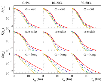
Figure 47: Same as fig. 41, but for a calculation without hadronic cascade.

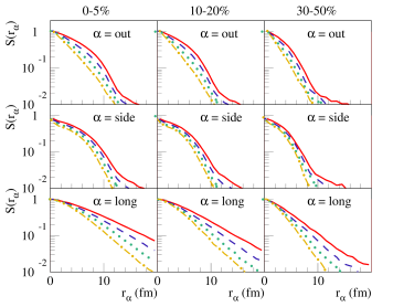
Figure 48: Same as fig. 41, but for a calculation where the hydro evolution is continued till freeze-out at 130 MeV (being the final freeze-out, no cascade afterwards).

The above discussion is important to understand the results concerning the femtoscopic radii for the different scenarios. The fitting procedure used to obtain the femtoscopic radii is based on the hypothesis that the source functions are Gaussians, the fit is therefore blind concerning the non-Gaussian tails. Due to the fact that the source function from the complete calculations and the full thermal scenario are identical apart from the tails, we expect similar results for these two scenarios, whereas the calculation without cascade should give smaller radii. This is exactly what we observe in fig. 49, where we show femtoscopic radii for the calculations without hadronic cascade (full line) and with hydrodynamical evolution till final freeze-out at 130 MeV (dashed). We observe always a decrease of the radii with $m_{T}$, but the dependence is somewhat weaker as compared to the data. But the magnitude in case of “no cascade” is very low compared to the two other scenarios, which are relatively close to each other, and to the data. Here the radii do not allow to discriminate between two scenarios which have nevertheless quite different source functions. This is a well-known problem, and there are methods to go beyond Gaussian parameterizations imag1 ; imag2 ; imag3 ; imag4 ; imag5 ; imag6 , but we will not discuss this any further.

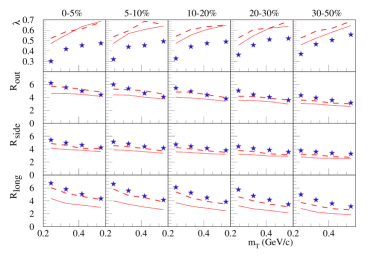
Figure 49: Same as fig. 40, but the calculations are done without hadronic cascade (full line) or with a hydrodynamic evolution through the hadronic phase with freeze-out at 130 MeV (dashed).

Although the Gaussian parameterizations represent only an incomplete information about the source functions, the centrality and transverse momentum dependence of the radii is nevertheless very useful. It is a necessary requirement for all models of soft physics to describe these radii correctly. There has been for many years an inconsistency, referred to as “HBT puzzle” hbt-puzzle . Although hydrodynamics descibes very successfully elliptical flow and to some extent particle spectra, one cannot get the femtoscopic radii correctly, when one uses “simple” hydrodynamics. Using transport models (and an event-by-event treatment) may help hbt6 . In hbt-puzzle , it has been shown that the puzzle can actually be solved by adding pre-equilibrium flow, taking a realistic equation of state, adding viscosity, using a more compact or more Gaussian initial energy density profile, and treating the two-pion wave function more accuratly. It has also been shown fto-th1 ; fto-th2 ; fto-th3 that using a Gaussian initial energy density profile, an early starting time (equivalent to initial flow), and a cross-over equation of state, and a late sudden freeze-out (at 145 MeV) helps to descibe the femtoscopic radii, and to some extent the spectra.

The scenario in fto-th1 ; fto-th2 ; fto-th3 is compatible with our scenario “hydrodynamical evolution till final freeze-out at 130MeV”, which allows us to get the femtoscopic radii correctly (see fig. 49), as well as some $v_{2}$ results and some spectra. One cannot describe, however, yields and spectra of lambdas and xis.

X Summary and conclusions

We presented a realistic treatment of the hydrodynamic evolution of ultrarelativistic heavy ion collisions, based on flux-tube initial conditions, event-by-event treatment, use of an efficient (3+1)D hydro code including flavor conservation, employment of a realistic equation-of-state, use of a complete hadron resonance table, and a hadronic cascade procedure after an hadronization from thermal matter at an early time.

Such an approach is able to describe simultaneously different soft observables such as femtoscopic radii, particle yields, spectra, and $v_{2}$ results. One obtains in a natural way a ridge structure when investigating $\Delta\eta\Delta\phi$ correlations, without adding a particular mechanism.

Considering such a multitude of observables, a clear picture of the collision dynamics emerges: a hydrodynamic evolution starting from initial flux-tube structures, till hadronization at an early time in the cross-over region of the phase transition, with subsequent hadronic rescatterings being quite important to understand the shapes of particle spectra.

Appendix A Pomeron structure

We define a so-called profile function function $G$ associated to a Pomeron exchange as

$$G(b)=\frac{1}{2s}2\mathrm{Im}\,\tilde{T}(b),$$ (36)

with $\tilde{T}$ being the Fourier transform of the Pomeron exchange scattering amplitude $T$,

$$\tilde{T}(b)=\frac{1}{4\pi^{2}}\int d^{2}q_{\bot}\,e^{-i\vec{q}_{\bot}\vec{b}}\,T(t),$$ (37)

using $t=-q_{\bot}^{2}$.

There are two contributions, a soft and a semi-hard one. The energy-momentum dependence of the semi-hard profile function may be expressed in terms of light cone momentum fractions as

$$G_{\mathrm{semi}}(x_{\mathrm{PE}}^{+},x_{\mathrm{PE}}^{-})=F_{\mathrm{part}}(x_{\mathrm{PE}}^{-})\,F_{\mathrm{part}}(x_{\mathrm{PE}}^{+})\,\omega(x_{\mathrm{PE}}^{+}x_{\mathrm{PE}}^{-}),$$ (38)

where the vertex function $F_{\mathrm{part}}$ is given as

$$F_{\mathrm{part}}(x)=\alpha_{\mathrm{F}}\,x^{\beta_{\mathrm{F}\,}},$$ (39)

using

$$\alpha_{\mathrm{F}}=s^{\varepsilon_{G}/2}\gamma_{h},\quad\beta_{\mathrm{F}}=\varepsilon_{G}-\alpha_{\mathrm{part}},$$ (40)

with parameters $\epsilon_{G}$, $\gamma_{h}$, $\alpha_{\mathrm{part}}$, and with

$$\omega(x_{\mathrm{PE}}^{+}x_{\mathrm{PE}}^{-}) = \int dx_{\mathrm{E}}^{+}dx_{\mathrm{E}}^{-}\int dt\sum_{ij}E^{i}(M_{F}^{2},x_{\mathrm{E}}^{+})E^{j}(M_{F}^{2},x_{\mathrm{E}}^{-})$$ (41)

$$\quad\times\frac{d\sigma_{ij}}{dt}(x_{\mathrm{PE}}^{+}x_{\mathrm{PE}}^{-}x_{\mathrm{E}}^{+}x_{\mathrm{E}}^{-}s,t).$$

The indices $i$ and $j$ refer to parton flavors, $M_{F}^{2}$ is the factorization scale (here $M_{F}^{2}=tu/s$). The quantity $d\sigma_{ij}/dt$ is the hard Born parton-parton scattering cross section, and $E^{i}(M_{F}^{2},x_{\mathrm{E}})$ the so-called complete evolution function, being a convolution of the soft and the QCD evolution,

$$E^{i}(M_{F}^{2},x_{\mathrm{E}}^{\pm}) =\sum_{k}\int dx_{\mathrm{soft}}^{\pm}dx_{\mathrm{QCD}}^{\pm}$$ (42)

$$E_{\mathrm{soft}}^{k}(x_{\mathrm{soft}}^{\pm})\,E_{\mathrm{QCD}}^{ki}(M_{F}^{2},x_{\mathrm{QCD}}^{\pm})\delta(x_{\mathrm{E}}^{\pm}-x_{\mathrm{soft}}^{\pm}x_{\mathrm{QCD}}^{\pm}).$$

The variables $x^{\pm}$ are light cone momentum fractions. The QCD evolution function is computed in the usual way based on the DGLAP equations,

$$\frac{dE_{\mathrm{QCD}}^{jm}\left(Q^{2},x\right)}{d\ln Q^{2}}=\sum_{k}\int_{x}^{1}\frac{dz}{z}\frac{\alpha_{s}}{2\pi}\tilde{P}_{k}^{m}\!(z)\>E_{\mathrm{QCD}}^{jk}\left(Q^{2},\frac{x}{z}\right),$$ (43)

with the initial condition

$$E_{\mathrm{QCD}}^{jm}\left(Q^{2}=Q_{0}^{2},x\right)=\delta_{j}^{m}\;\delta(1-x).$$ (44)

Here $\tilde{P}_{k}^{m}\!(z)$ are the usual Altarelli-Parisi splitting functions. One introduces the concept of “resolvable” parton emission, i.e. an emission of a final ($s$-channel) parton with a finite share of the parent parton light cone momentum $(1-z)>\epsilon=p_{\bot\textrm{res }}^{2\textrm{ }}/Q^{2}$ (with finite relative transverse momentum $p_{\bot}^{2}=$ $Q^{2}(1-z)$ $>p_{\bot\mathrm{res}\textrm{ }}^{2\textrm{ }}$) and use the so-called Sudakov form factor, corresponding to the contribution of any number of virtual and unresolvable emissions (i.e. emissions with $(1-z)<\epsilon$) ,

$$\Delta^{k}(Q_{0}^{2},Q^{2})=\exp\left\{\int_{Q_{0}^{2}}^{Q^{2}}\frac{dq^{2}}{q^{2}}\int_{1-\epsilon}^{1}dz\,\frac{\alpha_{s}}{2\pi}\,\tilde{P}_{k}^{k}(z)\right\}.$$ (45)

This can also be interpreted as the probability of no resolvable emission between $Q_{0}^{2}$ and $Q^{2}$. Then $E_{\mathrm{QCD}}^{jm}$ can be expressed via $\bar{E}_{\mathrm{QCD}}^{jm}$, corresponding to the sum of any number (but at least one) resolvable emissions, allowed by the kinematics:

$$E_{\mathrm{QCD}}^{jm}\left(Q^{2},x\right) =\delta_{j}^{m}\;\delta(1-x)\,\Delta^{j}(Q_{0}^{2},Q^{2})$$

$$+\bar{E}_{\mathrm{QCD}}^{jm}\left(Q_{0}^{2},Q^{2},x\right),$$ (46)

where $\bar{E}_{\mathrm{QCD}}^{jm}\left(Q_{0}^{2},Q^{2},x\right)$ satisfies the integral equation

$$\bar{E}_{\mathrm{QCD}}^{jm}\left(Q_{0}^{2},Q^{2},x\right)$$ (47)

$$=\int_{Q_{0}^{2}}^{Q2}\frac{dQ_{1}^{2}}{Q_{1}^{2}}\left[\sum_{k}\int_{x}^{1-\epsilon}\frac{dz}{z}\frac{\alpha_{s}}{2\pi}P_{k}^{m}\!(z)\>\bar{E}_{\mathrm{QCD}}^{jk}\left(Q_{0}^{2},Q_{1}^{2},\frac{x}{z}\right)\right.$$

$$+\left.\Delta^{j}(Q_{0}^{2},Q_{1}^{2})\frac{\alpha_{s}}{2\pi}P_{j}^{m}\!(x)\right]\Delta^{m}(Q_{1}^{2},Q^{2}).$$

Here $P_{j}^{k}\!(z)$ are the Altarelli-Parisi splitting functions for real emissions, i.e. without $\delta$-function and regularization terms at $z\rightarrow 1$. Eq. (47) can be solved iteratively, see nexus .

We define the soft contribution $G_{\mathrm{soft}}(s,b)$ as nexus

$$G_{\mathrm{soft}}(s,b)=\frac{2\gamma_{\mathrm{part}}^{2}}{\lambda_{\mathrm{soft}}\!(s/s_{0})}\left(\frac{s}{s_{0}}\right)^{\alpha_{\mathrm{soft}}-1}\exp\!\left(-\frac{b^{2}}{4\lambda_{\mathrm{soft}}\!(s/s_{0})}\right).$$ (48)

with

$$\lambda_{\mathrm{soft}}\!(z)=2R_{\mathrm{part}}^{2}+\alpha^{\prime}\!_{\mathrm{soft}}\ln\!z,$$ (49)

with parameters $\alpha_{\mathrm{soft}}$, $\alpha^{\prime}\!_{\mathrm{soft}}$ , $\gamma_{\mathrm{part}}$, $R_{\mathrm{part}}^{2}$, and a scale $s_{0}=1$GeV².

Appendix B Solving hydrodynamic equations

The algorithm is based on the Godunov method: one introduces finite cells and computes fluxes between cells using the (approximate) Riemann problem solution for each cell boundary. A relativistic HLLE solver is used to solve the Riemann problem. To achieve more accuracy in time, a predictor-corrector scheme is used for the second order of accuracy in time, i.e. the numerical error is $O(dt^{3})$, instead of $O(dt^{2})$. To achieve more accuracy in space, namely a second order scheme, the linear distributions of quantities (conservative variables) inside cells are used. The conservative quantities are $(e+p*v^{2})/(1-v^{2})$, $(e+p)*v/(1-v^{2})$ .

We rewrite equations in hyperbolic coordinates. These coordinates are suitable for the dynamical description at ultrarelativistic energies. It is convenient to write the equations in conservative form, the conservative variables are

$$\vec{Q}=\left(\begin{array}[]{c}Q_{\tau}\\ Q_{x}\\ Q_{y}\\ Q_{\eta}\\ Q_{B}\\ Q_{S}\\ Q_{Q}\end{array}\right)=\left(\begin{array}[]{c}\gamma^{2}(\epsilon+p)-p\\ \gamma^{2}(\epsilon+p)v_{x}\\ \gamma^{2}(\epsilon+p)v_{y}\\ \gamma^{2}(\epsilon+p)v_{\eta}\\ \gamma n_{B}\\ \gamma n_{S}\\ \gamma n_{Q}\end{array}\right),$$ (50)

where $n_{B}$, $n_{S}$, $n_{Q}$ are the densities of the conserved quantities $B$, $S$, and $Q$. The components $Q_{m}$ are conservative variables in the sense that the integral (discrete sum over all cells) of $Q_{m}$ gives the total energy, momentum, and the total $B$, $S$, and $Q$, which are conserved up to the fluxes at the grid boundaries. The velocities in these expressions are defined in the “Bjorken frame” related to velocities in laboratory frame as

$$v_{x} =v_{x}^{\mathrm{lab}}\cdot\frac{\cosh y}{\cosh(y-\eta_{s})}$$

$$v_{y} =v_{y}^{\mathrm{lab}}\cdot\frac{\cosh y}{\cosh(y-\eta_{s})}$$

$$v_{\eta} =\tanh(y-\eta_{s})$$ (51)

where $y=\frac{1}{2}\ln[(1+v_{z}^{\mathrm{lab}})/(1-v_{z}^{\mathrm{lab}})]$ is the longitudinal rapidity of the fluid element, $\eta_{s}=\frac{1}{2}\ln[(t+z)/(t-z)]$ is space-time rapidity. The full hydrodynamical equations are then

$$\partial_{\tau}\underbrace{\left(\begin{array}[]{c}Q_{\tau}\\ Q_{x}\\ Q_{y}\\ Q_{\eta}\\ Q_{B}\\ Q_{S}\\ Q_{Q}\end{array}\right)}_{\text{quantities}}+\vec{\nabla}\cdot\underbrace{\left(\begin{array}[]{c}Q_{\tau}\\ Q_{x}\\ Q_{y}\\ Q_{\eta}\\ Q_{B}\\ Q_{S}\\ Q_{Q}\end{array}\right)\vec{v}+\left(\begin{array}[]{c}\vec{\nabla}(p\cdot\vec{v})\\ \partial_{x}p\\ \partial_{y}p\\ \frac{1}{\tau}\partial_{\eta}p\\ 0\\ 0\\ 0\end{array}\right)}_{\text{fluxes}}+$$ (52)

$$\qquad\qquad\qquad+\underbrace{\left(\begin{array}[]{c}(Q_{\tau}+p)(1+v_{\eta}^{2})/\tau\\ Q_{x}/\tau\\ Q_{y}/\tau\\ 2Q_{\eta}/\tau\\ Q_{B}/\tau\\ Q_{S}/\tau\\ Q_{Q}/\tau\end{array}\right)}_{\text{sources}}=0$$

with $\vec{\nabla}=\left(\partial_{x},\ \partial_{y},\ \frac{1}{\tau}\partial_{\eta}\right)$.

We base our calculations on the finite-volume approach : we discretize the system on a fixed grid in the calculational frame and interpret $Q_{m,ijk}^{n}$ as average value over some space interval $\Delta V_{ijk}$, which is called a cell. The index $n$ refers to the discretized time.

The values of $Q_{m,ijk}^{n}$ are then updated after each time-step according to the fluxes on the cell interface during the time-step $\Delta t_{n}$. One has the following update formula :

$$Q_{m,ijk}^{n+1}= Q_{m,ijk}^{n}-\frac{\Delta t}{\Delta x_{1}}(F_{(i+1/2),jk}+F_{(i-1/2),jk})$$

$$-\frac{\Delta t}{\Delta x_{2}}(F_{i(,j+1/2),k}+F_{i,(j-1/2),k})$$ (53)

$$-\frac{\Delta t}{\Delta x_{3}}(F_{ij,(k+1/2)}+F_{ij,(k-1/2)}),$$

where $F$ is the average flux over the cell boundary, the indexes $+1/2$ and $-1/2$ correspond to the right and the left cell boundary in each direction. This is the base of the Godunov method Holt , which also implies that the distributions of variables inside a cell are piecewise linear (or piecewise parabolic etc, depending on the order of the numerical scheme), which forms a Riemann problem at each cell interface. Then the flux through each cell interface depends only on the solution of a single Riemann problem, supposing that the waves from the neighboring discontinuities do not intersect. The latter is satisfied with the Courant-Friedrichs-Lewy (CFL) condition CFL .

To solve the Riemann problems at each cell interface, we use the relativistic HLLE solver Schneider , which approximates the wave profile in the Riemann problem by a single intermediate state between two shock waves propagating away from the initial discontinuity. Together with the shock wave velocity estimate, in this approximation one can obtain an analytical dependence of the flux on the initial conditions for the Riemann problem, which makes the algorithm explicit.

We proceed then to construct a higher-order numerical scheme:

• in time: the predictor-corrector scheme is used for the second order accuracy in time, i.e. the numerical error is $O(dt^{3})$, instead of $O(dt^{2})$

• in space: in the same way, to achieve the second order scheme, the linear distributions of quantities (conservative variables) inside cells are used.

Some final remarks:

At each time-step, we compute and sum the fluxes for each cell with all its neighbors and update the value of conservative variables with the total flux. Thus, we do not use operator splitting (dimensional splitting) and thus avoid the numerical artifacts introduced by this method, e.g. artificial spatial asymmetry.

To treat grid boundaries, we use the method of ghost cells. We include 2 additional cells on either end of grid in each direction, and set the quantities in these cells at the beginning of each time-step. For simplicity, we set the quantities in ghost cells to be equal to these in the nearest "real" cell, thus implementing non-reflecting boundary conditions (outflow boundary). This physically correspond to boundary which does not reflect any wave, which is consistent with expansion into vacuum.

In our simulations we deal with spatially finite systems expanding into vacuum. Thus the computational grid in Eulerian algorithm must initially contain both system and surrounding vacuum. To account for the finite velocity of the expansion into the vacuum, which equals $c$ for an infinitesimal slice of matter on the boundary, we introduce additional (floating-point) variables in each cell which keep the extent of matter expansion within a cell, having the value unity for the complete cell, zero for a cell with vacuum only. The matter is allowed to expand in the next vacuum cell only if the current cell is filled with matter.

Appendix C resonance gas

Whereas for hadronization we employ the correct quantum statistics, we use the Boltzmann approximation for the calculation of the equation of state. This is reasonable even for pions at zero chemical potential, the excluded volume correction at nonzero chemical potentials is considerably bigger than the difference coming from quantum statistical treatment. We account for all well known hadrons made from u, d, s quarks from the PDG table For energy density, pressure and net charges we get :

$$\epsilon = \sum_{i}\!\!\frac{g_{i}}{2\pi^{2}}m_{i}^{2}T\left[3TK_{2}(\frac{m_{i}}{T})+\frac{m_{i}}{2}K_{1}(\frac{m_{i}}{T})\right]\exp(\mu_{i}/T)$$ (54)

$$\qquad\qquad\qquad\cdot$$

$$p = \sum_{i}\frac{g_{i}}{2\pi^{2}}m_{i}^{2}T^{2}\cdot K_{2}(\frac{m_{i}}{T})\cdot\exp(\mu_{i}/T)$$ (55)

$$n_{B} = \sum_{i}B_{i}\frac{g_{i}}{2\pi^{2}}m_{i}^{2}T\cdot K_{2}(\frac{m_{i}}{T})\cdot\exp(\mu_{i}/T)$$ (56)

$$n_{Q} = \sum_{i}Q_{i}\frac{g_{i}}{2\pi^{2}}m_{i}^{2}T\cdot K_{2}(\frac{m_{i}}{T})\cdot\exp(\mu_{i}/T)$$ (57)

$$n_{S} = \sum_{i}S_{i}\frac{g_{i}}{2\pi^{2}}m_{i}^{2}T\cdot K_{2}(\frac{m_{i}}{T})\cdot\exp(\mu_{i}/T)$$ (58)

with

$$\mu_{i}=B_{i}\mu_{B}+Q_{i}\mu_{Q}+S_{i}\mu_{S},$$ (59)

where $\mu_{B}$, $\mu_{S}$, $\mu_{Q}$ are the chemical potentials associated to $B$, $S$, $Q$, and $B_{i}$, $S_{i}$, $Q_{i}$ are the baryon charge, strangeness, and the electric charge of i-th hadron state, $g_{i}=(2J_{i}+1)$ is degeneracy factor.

For large baryon chemical potential the EoS correction for the deviations from ideal gas due to particle interactions becomes more important. We employ this correction in a form of an excluded volume effect, like a Van der Waals hard core correction. According to this prescription,

$$p(T,\mu_{B},\mu_{Q},\mu_{S})=\sum\limits_{i}p_{i}^{\text{boltz}}(T,\tilde{\mu}_{i}),$$ (60)

$$\tilde{\mu}_{i}=\mu_{i}-v_{i}\cdot p\,.$$ (61)

If one supposes equal volume $v_{i}=v$ for all particle species, then the correction can be computed as a solution $p(T,\mu_{B},\mu_{Q},\mu_{S})$ of a fairly simple, however transcendental equation,

$$p(T,\mu_{B},\mu_{Q},\mu_{S})=p^{\text{boltz}}(T,\mu_{B},\mu_{Q},\mu_{S})e^{-vp(T,\mu_{B},\mu_{Q},\mu_{S})/T}$$ (62)

We take the value $v\approx 1.44\ fm^{3}$, which corresponds to the hard core radius $r=0.7fm$.

Appendix D Ideal QGP

In this ideal phase, matter is made from massless $u$, $d$ quarks and massive $s$-quark (+antiquarks). Due to the possibility of a large strange quark chemical potential, comparable to its mass $m_{s}=120\,\mathrm{MeV}$ which is taken in our calculations, we perform the integration of the strange quark contribution to thermodynamic quantities exactly, without Boltzmann or zero-mass approximation. So we have

$$p =\frac{g_{l}}{6\pi^{2}}\left[\frac{1}{4}\mu_{u}^{4}+\frac{\pi^{2}}{2}\mu_{u}^{2}T^{2}+\frac{7\pi^{4}T^{4}}{60}\right]$$ (63)

$$+\frac{g_{l}}{6\pi^{2}}\left[\frac{1}{4}\mu_{d}^{4}+\frac{\pi^{2}}{2}\mu_{d}^{2}T^{2}+\frac{7\pi^{4}T^{4}}{60}\right]+$$

$$+p_{s}(T,\mu_{s})+p_{\bar{s}}(T,\mu_{s})+\frac{g_{g}\pi^{2}}{90}T^{4}-B,\ \text{}$$

with $p_{\bar{s}}(T,\mu_{s})=p_{s}(T,-\mu_{s})$, and

$$p_{s}(T,\mu_{s})=\frac{g_{l}T}{2\pi^{2}}\int_{0}^{\infty}\!\!\!p^{2}\ln\left[1\!+\!\exp\left(\frac{1}{T}\sqrt{p^{2}+m_{s}^{2}}+\!\frac{\mu_{s}}{T}\right)\right]dp,$$ (64)

where we use the degeneracy factors $g_{l}=6$ for light quarks, $g_{g}=16$ for gluons, and a bag constant $B=0.38\ \mathrm{GeV}/\mathrm{fm^{3}}$. Quark chemical potentials are

$$\mu_{u} =\frac{1}{3}\mu_{B}+\frac{2}{3}\mu_{Q}\,,$$ (65)

$$\mu_{d} =\frac{1}{3}\mu_{B}-\frac{1}{3}\mu_{Q}\,,$$ (66)

$$\mu_{s} =\frac{1}{3}\mu_{B}-\frac{1}{3}\mu_{Q}-\mu_{S}\,.$$ (67)

Using the relations $n_{i}=\partial p/\partial\mu_{i}$, $s=\partial p/\partial T$, $\varepsilon=Ts+\sum\mu_{i}n_{i}-p$, we get

$$\epsilon =3(p-p_{s}-p_{\bar{s}}+B)+\epsilon_{s}+\epsilon_{\bar{s}}+B$$ (68)

$$n_{B} =\frac{1}{3}\frac{g_{l}}{6\pi^{2}}\left[\mu_{u}^{3}+\pi^{2}\mu_{u}T^{2}+\mu_{d}^{3}+\pi^{2}\mu_{d}T^{2}\right]+$$ (69)

$$+\frac{1}{3}\left[n_{s}(T,\mu_{s})-n_{\bar{s}}(T,-\mu_{s})\right]$$

$$n_{Q} =\frac{1}{3}\frac{g_{l}}{6\pi^{2}}\left[2\mu_{u}^{3}+2\pi^{2}\mu_{u}T^{2}-\mu_{d}^{3}-\pi^{2}\mu_{d}T^{2}\right]-$$ (70)

$$-\frac{1}{3}\left[n_{s}(T,\mu_{s})-n_{\bar{s}}(T,-\mu_{s})\right]$$

$$n_{S} =-\left[n_{s}(T,\mu_{s})-n_{\bar{s}}(T,-\mu_{s})\right]$$ (71)

with $\epsilon_{\bar{s}}(T,\mu_{s})=\epsilon_{s}(T,-\mu_{s})$, and

$$\epsilon_{s}(T,\mu_{s}) =\frac{g_{l}}{2\pi^{2}}\int\limits_{0}^{\infty}\frac{p^{2}\sqrt{p^{2}+m_{s}^{2}}}{\exp\left(\frac{1}{T}\sqrt{p^{2}+m_{s}^{2}}-\frac{\mu_{s}}{T}\right)+1}dp,$$ (72)

$$n_{s}(T,\mu_{s}) =\frac{g_{l}}{2\pi^{2}}\int\limits_{0}^{\infty}\frac{p^{2}}{\exp\left(\frac{1}{T}\sqrt{p^{2}+m_{s}^{2}}-\frac{\mu_{s}}{T}\right)+1}dp.$$ (73)

Appendix E Plasma hadronization

We parametrize the hadronization hyper-surface $x^{\mu}=x^{\mu}(\tau,\varphi,\eta)$ as

$$x^{0}=\tau\cosh\eta,\;x^{1}=r\cos\varphi,\;x^{2}=r\sin\varphi,\;x^{3}=\tau\sinh\eta,$$ (74)

with $r=r(\tau,\varphi,\eta)$ being some function of the three parameters $\tau,\>\varphi,\>\eta$. The hypersurface element is

$$d\Sigma_{\mu}=\varepsilon_{\mu\nu\kappa\lambda}\frac{\partial x^{\nu}}{\partial\tau}\frac{\partial x^{\kappa}}{\partial\varphi}\frac{\partial x^{\lambda}}{\partial\eta}d\tau d\varphi d\eta,$$ (75)

with $\varepsilon^{\mu\nu\kappa\lambda}=-\varepsilon_{\mu\nu\kappa\lambda}=1$. Computing the partial derivatives $\partial x^{\mu}/d\alpha$, with $\alpha=\tau,$ $\varphi$, $\eta$, one gets

$$d\Sigma_{0} = \left\{-r\frac{\partial r}{\partial\tau}\tau\cosh\eta+r\frac{\partial r}{\partial\eta}\sinh\eta\right\}d\tau d\varphi d\eta,$$ (76)

$$d\Sigma_{1} = \left\{\quad\quad\frac{\partial r}{\partial\varphi}\tau\sin\varphi+r\,\tau\cos\varphi\;\right\}d\tau d\varphi d\eta,$$ (77)

$$d\Sigma_{2} = \left\{\quad\,-\frac{\partial r}{\partial\varphi}\tau\cos\varphi+r\,\tau\sin\varphi\;\right\}d\tau d\varphi d\eta,$$ (78)

$$d\Sigma_{3} = \left\{\quad r\frac{\partial r}{\partial\tau}\tau\sinh\eta-r\frac{\partial r}{\partial\eta}\cosh\eta\right\}d\tau d\varphi d\eta.$$ (79)

Cooper-Frye hadronization amounts to calculating

$$E\frac{dn}{d^{3}p}=\int d\Sigma_{\mu}p^{\mu}f(up),$$

with $u$ being the flow four-velocity in the global frame, which can be expressed in terms of the four-velocity $\tilde{u}$ in the “Bjorken frame” as

$$u^{0} = \tilde{u}\,^{0}\cosh\eta+\tilde{u}\,^{3}\sinh\eta\,,$$ (80)

$$u^{1} = \tilde{u}\,^{1}\,,$$ (81)

$$u^{2} = \tilde{u}\,^{2}\,,$$ (82)

$$u^{3} = \tilde{u}\,^{0}\sinh\eta+\tilde{u}\,^{3}\cosh\eta\,.$$ (83)

In a similar way one may express $p$ in terms of $\tilde{p}$ in the Bjorken frame. Using $\gamma=\tilde{u}\,^{0}$ and the flow velocity $v^{\mu}=\tilde{u}\,^{\mu}/\gamma$, we get

$$\frac{dn}{dyd\phi dp_{\bot}}=$$ (84)

$$p_{\bot}\int\left\{-r\frac{\partial r}{\partial\tau}\tau\,\tilde{p}\,^{0}+\,r\,\tau\,\tilde{p}\,^{r}+\,\frac{\partial r}{\partial\varphi}\tau\tilde{p}\,^{t}\,-\,r\frac{\partial r}{\partial\eta}\tilde{p}\,^{3}\right\}f(x,p),$$

with $\tilde{p}\,^{r}=\tilde{p}\,^{1}\cos\varphi+\tilde{p}\,^{2}\sin\varphi$ and $\tilde{p}\,^{t}=\tilde{p}\,^{1}\sin\varphi-\tilde{p}\,^{2}\cos\varphi$ being the radial and the tangential transverse momentum components. Our Monte Carlo generation procedure is based on based on the invariant volume element moving through the FO surface,

$$dV^{*}=d\Sigma_{\mu}u^{\mu}=w\,d\tau d\varphi d\eta,$$ (85)

with

$$w=\gamma\left\{-r\frac{\partial r}{\partial\tau}\tau\,+\,r\,\tau\,v^{r}\,+\,\frac{\partial r}{\partial\varphi}\tau v^{t}\,-\,r\frac{\partial r}{\partial\eta}v^{3}\right\},$$ (86)

and with $v^{r}=v^{1}\cos\varphi+v^{2}\sin\varphi$ and $v^{t}=v^{1}\sin\varphi-v^{2}\cos\varphi$ being the radial and the tangential transverse flow. Freeze out is the done as follows (equivalent to Cooper-Frye): the proposal of isotropic particles production in the local rest frame as

$$dn_{i}=\alpha\,d^{3}p^{*}\,dV^{*}\,f_{i}(E^{*}),$$ (87)

is accepted with probability

$$\kappa=\frac{d\Sigma_{\mu}\,p^{\mu}}{\alpha\,dV^{*}E^{*}}.$$ (88)

In case of acceptance, the momenta are boosted to the global frame.

Appendix F Pair wave function for femtoscopy applications

In case of identical particles, we use

$$\Phi(\mathbf{q^{\prime},r^{\prime}})=\frac{1}{\sqrt{2}}\left(\phi(\mathbf{k^{\prime},r^{\prime}})\pm\phi(-\mathbf{k^{\prime},r^{\prime}})\right),$$ (89)

and for non-identical particles

$$\Phi(\mathbf{q^{\prime},r^{\prime}})=\phi(\mathbf{k^{\prime},r^{\prime}}),$$ (90)

with $\mathbf{k^{\prime}}=\mathbf{q^{\prime}}/2$. In the simplest case, neglecting final state ineteractions, one has simply

$$\phi(-\mathbf{k^{\prime},r^{\prime}})=\exp(-i\mathbf{k^{\prime},r^{\prime}})\,,$$ (91)

otherwise the non-symmetrized wavefunction is given as (see eq. (89) of hbt-lednicki )

$$\phi(-\mathbf{k^{\prime},r^{\prime}})=\exp(i\delta_{c})\,\sqrt{A_{c}(\eta)}$$ (92)

$$\qquad\times\,\left[\exp(-i\mathbf{k^{\prime},r^{\prime}})\,F(-i\eta,1,i\xi)+f_{c}(k^{\prime})\frac{\tilde{G}(\rho,\eta)}{r^{\prime}}\right],$$

with $\xi=\mathbf{k^{\prime}r^{\prime}}+q^{\prime}r^{\prime}$, $\;\rho=k^{\prime}r^{\prime}$,$\;\eta=(k^{\prime}a)^{-1}$. The quantity $\;a=(\mu z_{1}z_{2}e^{2})^{-1}$is the Bohr radius of the pair, in case of pion-pion one has 387 fm. Furthermore, $\delta_{c}=\mathrm{arg}\,\Gamma(1+i\eta)$ is the Coulomb s-wave phase shift, $A_{c}(\eta)=2\pi\eta\left(\exp(2\pi\eta)-1\right)^{-1}$ is the Coulomb penetration factor,

$$F(\alpha,1,z)=1+\alpha z/1!^{2}+\alpha(\alpha+1)z^{2}/2!^{2}+...$$ (93)

is the confluent hypergeometric function,

$$\tilde{G}(\rho,\eta) =P(\rho,\eta)+2\eta\rho\,B(\rho,\eta)$$ (94)

$$\qquad\times\left[\ln|2\eta\rho|+2C-1+\chi(\eta)\right],$$

with the Euler constant $C=0.5772$, and

$$B(\rho,\eta)=\sum_{s=0}^{\infty}B_{s},\;P(\rho,\eta)=\sum_{s=0}^{\infty}P_{s},$$ (95)

with $B_{0}=1$, $B_{1}=\eta\rho$, $P_{0}=1$, $P_{1}=0$, and

$$(n+1)(n+2)B_{n+1} =2\eta\rho B_{n}-\rho^{2}B_{n-1},$$ (96)

$$n(n+1)P_{n+1} =2\eta\rho P_{n}-\rho^{2}P_{n-1}$$ (97)

$$\quad-(2n+1)2\eta\rho B_{n}.$$

The function $\chi$ is given as

$$\chi(\eta)=h(\eta)+iA_{c}(\eta)/(2\eta),$$ (98)

where $h$ is expressed in terms of the digamma function $\psi(z)=\Gamma^{\prime}(z)/\Gamma(z)$ as

$$h(\eta)=\frac{1}{2}\left[\psi(i\eta)+\psi(-i\eta)-\ln(\eta^{2})\right].$$ (99)

The amplitude $f_{c}$ can be written as

$$f_{c}(k^{\prime})=f(k^{\prime})/A_{c}(\eta),$$ (100)

where $f(k^{\prime})$ is the amplitude of the low energy s-wave elastic scattering due to the short range interaction renormalized by the long-range Coulomb forces. We may write

$$f_{c}(k^{\prime})=\left(K^{-1}-\frac{2\chi(\eta)}{a}\right)^{-1},$$ (101)

with hbt-gasser

$$K=\frac{2}{\sqrt{s}}\,\frac{s_{\mathrm{th}}-s_{0}}{s-s_{0}}\sum_{j=0}^{3}A_{j}\left(\frac{2k^{\prime}}{\sqrt{s_{\mathrm{th}}}}\right)^{2j},$$ (102)

$$s=\left(\sum_{i=1}^{2}\sqrt{m_{i}^{2}+k^{\prime 2}}\right)^{2},\quad s_{\mathrm{th}}=(m_{1}+m_{2})^{2},$$ (103)

with the parameters as given in hbt-gasser .

References

- (1) STAR Collaboration: J. Adams, et al, Nucl. Phys. A757:102, 2005
- (2) PHENIX Collaboration, K. Adcox, et al, Nucl. Phys. A757:184-283, 2005
- (3) BRAHMS Collaboration, I. Arsene et al., Nucl. Phys. A757:1-27, 2005
- (4) PHOBOS Collaboration, B.B. Back et al., Nucl. Phys. A757:28-101, 2005
- (5) P. Huovinen, in Quark-Gluon Plasma 3, eds. R. C. Hwa and X. N. Wang (World Scientific, Singapore, 2004)
- (6) P. F. Kolb and U. Heinz, in Quark-Gluon Plasma 3, eds. R. C. Hwa and X. N. Wang (World Scientific, Singapore, 2004)
- (7) U. W. Heinz and P. F. Kolb, Nucl. Phys. A 702 (2002) 269
- (8) P. Huovinen, P. F. Kolb, U. W. Heinz, P. V. Ruuskanen and S. A. Voloshin, Phys. Lett. B 503 (2001) 58
- (9) U. W. Heinz, P. F. Kolb, Nucl. Phys. A702:269 (2002)
- (10) P. Braun-Munzinger, K. Redlich, J. Stachel, arXiv:nucl-th/0304013, in Quark Gluon Plasma 3, eds. R. C. Hwa and Xin-Nian Wang, World Scientific Publishing;
- (11) A. Andronic, P. Braun-Munzinger, J. Stachel, Phys.Lett.B673:142,2009
- (12) A. Andronic, P. Braun-Munzinger, J. Stachel, arXiv:0901.2909, Acta Phys.Polon.B40:1005-1012,2009
- (13) F. Becattini, J. Manninen, J.Phys.G35:104013, 2008
- (14) F. Becattini, R. Fries, arXiv:0907.1031, accepted for publication in Landolt-Boernstein Volume 1-23A
- (15) Giorgio Torrieri, Johann Rafelski, arXiv:nucl-th/0212091, Phys.Rev. C68 (2003) 034912
- (16) J. Cleymans, B. Kampfer, S. Wheaton, Phys. Rev. C65:027901, 2002
- (17) T. Hirano and K. Tsuda, Phys. Rev. C 66 (2002) 054905T.
- (18) T. Hirano, U.W.Heinz, D. Kharzeev, R. Lacey and Y. Nara, Phys. Lett. B 636 (2006) 299
- (19) T. Hirano, U. Heinz, D. Kharzeev, R. Lacey, Y. Nara, Phys.Rev.C77: 044909,2008,
- (20) D. Teaney, J. Lauret and E. V. Shuryak, Phys. Rev. Lett.86, 4783 (2001)
- (21) C. Nonaka and S. A. Bass, Nucl. Phys. A 774, 873 (2006); and Phys. Rev. C 75, 014902 (2007)
- (22) Y.Hama, T.Kodama and O.Socolowski Jr. Braz. J. Phys. 35 (2005) 24
- (23) R. Andrade, F. Grassi, Y. Hama, T. Kodama, O. Socolowski Jr, Phys. Rev. Lett. 97:202302, 2006
- (24) R.P.G. Andrade, F. Grassi, Y. Hama, T. Kodama, W.L. Qian, Phys.Rev.Lett.101:112301,2008
- (25) H. J. Drescher, M. Hladik, S. Ostapchenko, T. Pierog and K. Werner, Phys. Rept. 350, 93, 2001
- (26) H. J. Drescher, S. Ostapchenko, T. Pierog, and K.Werner, Phys.Rev.C65:054902, 2002, hep-ph/0011219
- (27) (Mini)symposium on Proton-Proton Interactions, February 14 - 17 2010, Frankfurt am Main, Germany. Results to be published
- (28) T. Pierog, Klaus Werner. Phys. Rev. Lett. 101, 171101 (2008), astro-ph/0611311
- (29) P. Romatschke, U. Romatschke, Phys. Rev. Lett. 99 172301, 2007
- (30) H. Song and U. Heinz, Phys. Lett. B 658 279, 2008
- (31) K. Dusling and D. Teaney, Phys. Rev. C 77 034905, 2008
- (32) M. Luzum and P. Romatschke, Phys. Rev. C 78 034915, 2008
- (33) D. Molnar and P. Huovinen, J. Phys. G: Nucl.Part.Phys. 35 1041, 2008
- (34) Huichao Song, Ulrich W. Heinz, J. Phys. G36:064033, 2009
- (35) B. Andersson, G. Gustafson, G. Ingelman, and T. Sjostrand, Phys. Rept. 97, 31, 1983
- (36) K. Werner, Phys. Rep. 232, 87, 1993
- (37) A. Capella, U. Sukhatme, C.-I. Tan, and J. {Tran Thanh Van}, Phys. Rept. 236, 225, 1994
- (38) L.D. McLerran, R. Venugopalan, Phys. Rev. D 49, 2233 (1994). ibid. D49, 3352 (1994); D 50, 2225 (1994)
- (39) Yu.V. Kovchegov, Phys. Rev. D 54, 5463 (1996)
- (40) E. Iancu, R. Venugopalan, Quark Gluon Plasma 3, Eds. R.C. Hwa, X.N.Wang, World Scientific, hep-ph/0303204
- (41) A. Kovner, L.D. McLerran, H. Weigert, Phys. Rev. D 52, 3809 (1995); ibid., D 52, 6231 (1995).
- (42) F. Gelis, E. Iancu, J. Jalilian-Marian, R. Venugopalan, arXiv:1002.0333, submitted to the Annual Review of Nuclear and Particle Sciences
- (43) Adrian Dumitru, Francois Gelis, Larry McLerran, Raju Venugopalan, arXiv:0804.3858, Nucl.Phys.A810:91,2008
- (44) BRAHMS collaboration, I. G. Bearden, Phys Rev Lett 94, 162301 (2005)
- (45) BRAHMS collaboration, I. Arsene, Phys. Rev. C 72, 014908 (2005)
- (46) STAR Collaboration, J.Adams, et al, Phys. Rev. Lett. 98 (2007) 62301, nucl-ex/0606014
- (47) Klaus Werner, Fu-Ming Liu, Tanguy Pierog, Phys. Rev. C 74, 044902 (2006), arXiv: hep-ph/0506232
- (48) M. Bleicher, F. M. Liu, A. Ker nen, J. Aichelin, S.A. Bass, F. Becattini, K. Redlich, and K. Werner, Phys.Rev.Lett.88, 202501, 2002.
- (49) F.M. Liu, J.Aichelin, M.Bleicher, H.J. Drescher, S. Ostapchenko, T. Pierog, and K. Werner, Phys. Rev. D67, 034011, 2003
- (50) Y. Nambu, Proc. Intl. Conf. on Symmetries and Quark Models, Wayne State Univ., 1969
- (51) J. Scherk, Rev. Mod. Phys. 47, 123 (1975)
- (52) C. Rebbi, Phys. Rep. 12 (1974) 1
- (53) X. Artru and G. Mennessier, Nucl. Phys. B70, 93 (1974)
- (54) X. Artru, Phys. Rep. 97, 147 (1983)
- (55) D. A. Morris, Nucl. Phys. B288, 717, 1987
- (56) K. Werner, Phys. Rev. Lett. 98, 152301 (2007)
- (57) J. Aichelin, K. Werner, Phys.Rev.C79:064907, 2009
- (58) F. Becattini, J. Manninen, Phys.Lett.B673:19-23, 2009
- (59) T. Kodama, private communication
- (60) Yu.M. Sinyukov, Act. Phys. Pol. B 37, 3343 (2006)
- (61) M. Gyulassy, Iu.A. Karpenko, A.V. Nazarenko, Yu.M. Sinyukov, Braz. J. Phys. 37, 1031 (2007)
- (62) Yu.M. Sinyukov, Iu.A. Karpenko, A.V. Nazarenko, J. Phys. G 35, 104071 (2008)
- (63) Yu.M. Sinyukov , A.N. Nazarenko , Iu.A. Karpenko, Acta Phys.Polon.B40:1109-1118, 2009
- (64) W. Broniowski, W. Florkowski, M. Chojnacki, A. Kisiel, Acta Phys. Polon. B40:979-986, 2009
- (65) S. Pratt,, Nucl. Phys. A830:51C-57C, 2009, arXiv:0907.1094
- (66) Y. Aoki, Z. Fodor, S.D. Katz , K.K. Szabo, JHEP 0601:089, 2006
- (67) M. Bleicher et al., J. Phys. G25 (1999) 1859
- (68) H. Petersen, J. Steinheimer, G. Burau, M. Bleicher and H. Stocker, Phys. Rev. C78 (2008) 044901
- (69) J. Takahashi et al. Phys. Rev.Lett. 103 (2009) 242301
- (70) R.P.G. Andrade, F. Grassi, Y. Hama, W.L. Qian, arXiv:0912.0703
- (71) STAR Collaboration, B. Abelev et al., Phys. Rev. C 80 (2009) 64192
- (72) J.-Y. Ollitrault, Nucl. Phys. A 638 (1998) 195c
- (73) PHOBOS Collaboration, B. Alver, et al, Phys. Rev. Lett. 98, 242302 (2007), nucl-ex/0610037
- (74) J. Aichelin, K. Werner, to be published in the proceedings of SQM 2009
- (75) K. Werner, T. Hirano, Iu. Karpenko, T. Pierog, S. Porteboeuf, M. Bleicher, S. Haussler, J. Phys. G: Nucl. Part. Phys. 36 (2009) 064030, arXiv:0907.5529
- (76) Pasi Huovinen, Nucl.Phys.A761:296-312,2005, nucl-th/0505036
- (77) R.S. Bhalerao, J.-P. Blaizot , N. Borghini, J.-Y. Ollitrault, Phys. Lett. B627:49-54, 2005
- (78) PHOBOS Collaboration, Phys.Rev. C72 (2005) 051901, and Phys.Rev.Lett. 94 (2005) 122303
- (79) STAR Collaboration, J. Adams et al, Phys. Rev. Lett. 92 (2004) 052302, nucl-ex/0306007
- (80) PHENIX Collaboration, S.S. Adler et al, Phys.Rev.Lett. 91 (2003) 182301, nucl-ex/0305013
- (81) PHENIX Collaboration, S. Afanasiev et al, Phys. Rev. Lett. 99 (2007) 052301, nucl-ex/0703024
- (82) A. Adil, H. J. Drescher, A. Dumitru, A. Hayashigaki and Y. Nara, Phys. Rev. C 74, 044905 (2006).
- (83) H.-J. Drescher , Adrian Dumitru, Arata Hayashigaki, Yasushi Nara, Phys.Rev.C74:044905,2006
- (84) Tables of curves kindly provided by T. Hirano
- (85) BRAHMS Collaboration, I. G. Bearden et al., Phys. Rev. Lett. 93, 102301 (2004); PhD thesis, Djamel Ouerdane, Univ. of Copenhagen, 2003; Phys. Rev. Lett. 94, 162301 (2005)
- (86) STAR Collaboration, J. Adams, et al, Phys.Rev.Lett. 92 (2004) 112301, nucl-ex/0310004
- (87) PHENIX Collaboration, S.S. Adler et al., Phys. Rev. C69 (2004) 034909, nucl-ex/0307022
- (88) PHOBOS Collaboration, B.B.Back et al, Phys.Rev. C70 (2004) 021902, nucl-ex/0405027
- (89) G. I. Kopylov and M. I. Podgoretsky, Sov. J. Nucl. Phys. 15, 219 (1972). [2]
- (90) G. I. Kopylov and M. I. Podgoretsky, Sov. J. Nucl. Phys. 18, 336 (1974).
- (91) S. Pratt, Phys. Rev. Lett. 53:1219-1221,1984
- (92) M. A. Lisa, Scott Pratt , Ron Soltz, Urs Wiedemann, Ann. Rev. Nucl. Part.Sci.55:357-402, 2005, nucl-ex/0505014
- (93) A. Kisiel, W. Florkowski, W. Broniowski, Phys.Rev.C73:064902,2006, nucl-th/0602039
- (94) R. Lednicky, Physics of Particles and Nuclei 40 (2009) 307
- (95) G. F. Bertsch, M. Gong, and M. Tohyama, Phys. Rev. C 37, 1896 (1988)
- (96) S. Pratt, Phys. Rev. D 33, 1314 (1986)
- (97) S. Chapman, P. Scotto, and U. W. Heinz, Phys. Rev. Lett. 74, 4400 (1995).
- (98) STAR collaboration, J. Adams et al., Phys. Rev. C 71 (2005) 44906
- (99) M. Lisa, private communication, 26.3.2010
- (100) G. Verde et al. Phys. Rev. C65:054609, 2002
- (101) S. Y. Panitkin et al. Phys. Rev. Lett. 87:112304, 2001
- (102) D. A. Brown and P. Danielewicz. Phys. Rev. C64:014902, 2001
- (103) David A. Brown, Fu-qiang Wang, and Pawel Danielewicz. Phys. Lett. B470:33–38, 1999
- (104) D.A. Brown and P. Danielewicz. Phys. Lett. B398:252–258, 1997
- (105) P. Chung et al. Phys. Rev. Lett. 91:162301, 2003
- (106) W. Broniowski, M. Chojnacki, W. Florkowski, A. Kisiel, Phys.Rev.Lett.101:022301, 2008
- (107) W. Florkowski , W. Broniowski , M. Chojnacki , A. Kisiel, Acta Phys.Polon.B40:1093-1098, 2009
- (108) W. Florkowski , W. Broniowski, M. Chojnacki, A. Kisiel, Nucl.Phys.A830:821c-824c, 2009
- (109) M. Holt, "Numerical methods in fluid dynamics", Springer Series in Comput. Physics (Springer, Berlin, 1977).
- (110) R. Courant, K. Friedrichs and H. Lewy, "On the partial difference equations of mathematical physics", IBM Journal, March 1967, pp. 215-234.
- (111) V. Schneider et al., J. Comput. Phys. 105 (1993) 92.
- (112) G. Colangelo, J. Gasser, H. Leutwyler, Nucl. Phys. B603 (2001) 125